JS 115- Population Genetics- Assessing the Strength of the Evidence

I. Pre class activitiesa. Quizb. Review Assignments and Schedulesc. Return and Review Examsd. Break

II. Learning Objectives (Rudin Ch 8- Butler Ch 19 and 20)

a. Define Genetic Concordance or “Match”Continuous Alleles vs Discrete allele system review

b. Understand the evaluation of Results- Where the rubber meets the road! Genetic concordance under 3 circumstances

c. Frequency estimate calculations- The strength of the result of the inference of common source between the biological evidence nad reference donor.

1. Hardy-Weinberg Equilibrium-Definition2. HWE- Assumptions-3. In class “mating” under HWE /w selection

and migration!4. Linkage equilibrium frequencies

Assignments

• Read chapters Butler 8-10 and Inman C9

• Extra credit: – Read SWGDAM STR Interpretation Guidelines– http://www.fbi.gov/hq/lab/fsc/backissu/july200

0/strig.htm– Write 500 word summary with 3Q and 3A

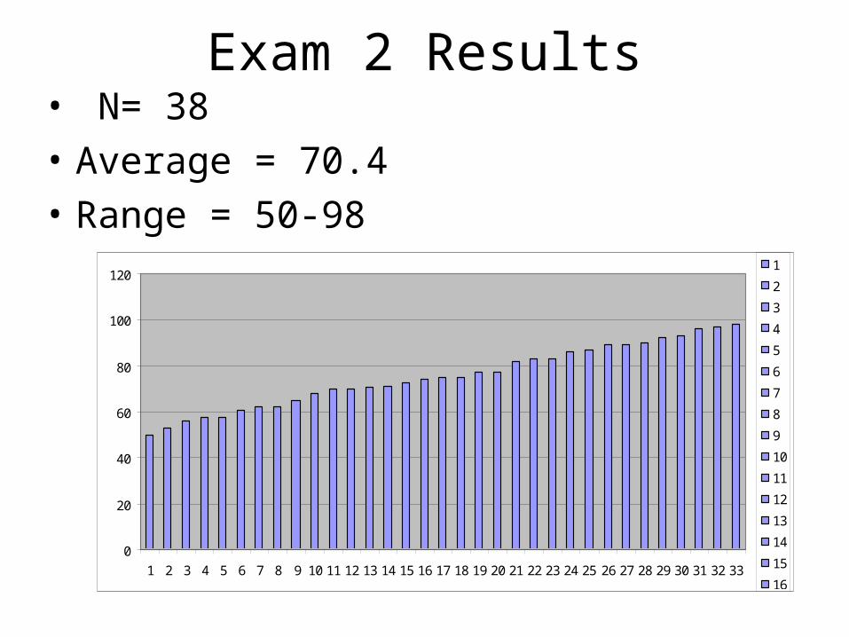
Exam 2 Results• N= 38

• Average = 70.4

• Range = 50-98

0

20

40

60

80

100

120

1 2 3 4 5 6 7 8 9 10 11 12 13 14 15 16 17 18 19 20 21 22 23 24 25 26 27 28 29 30 31 32 33

1

2

3

4

5

6

7

8

9

10

11

12

13

14

15

16

17

Genetic Concordance or “Match”

• Scientists: Match- reserved to no significant differences observed between 2 samples in the particular test(s) conducted. May be different but the test failed to reveal.

• DNA tests are limited to a very small % of the human genome

• Public- Match connotes absolute individualization. Therefore conclusion of “genetic concordance simply describes the fact that two samples show the same genotypes.

Continuous vs Discrete alleles

• Continuous alleles : RFLP: continuous alleles are not resolved- e.g. 99 vs 100 repeats are too similar

• Discrete alleles- PCR: method clearly differentiates the types- exact number of repeats can be determined

• Analogy: Continuous alleles- Too close to call the difference between the two runnersDiscrete: Every runner has exact speed(size) detected.

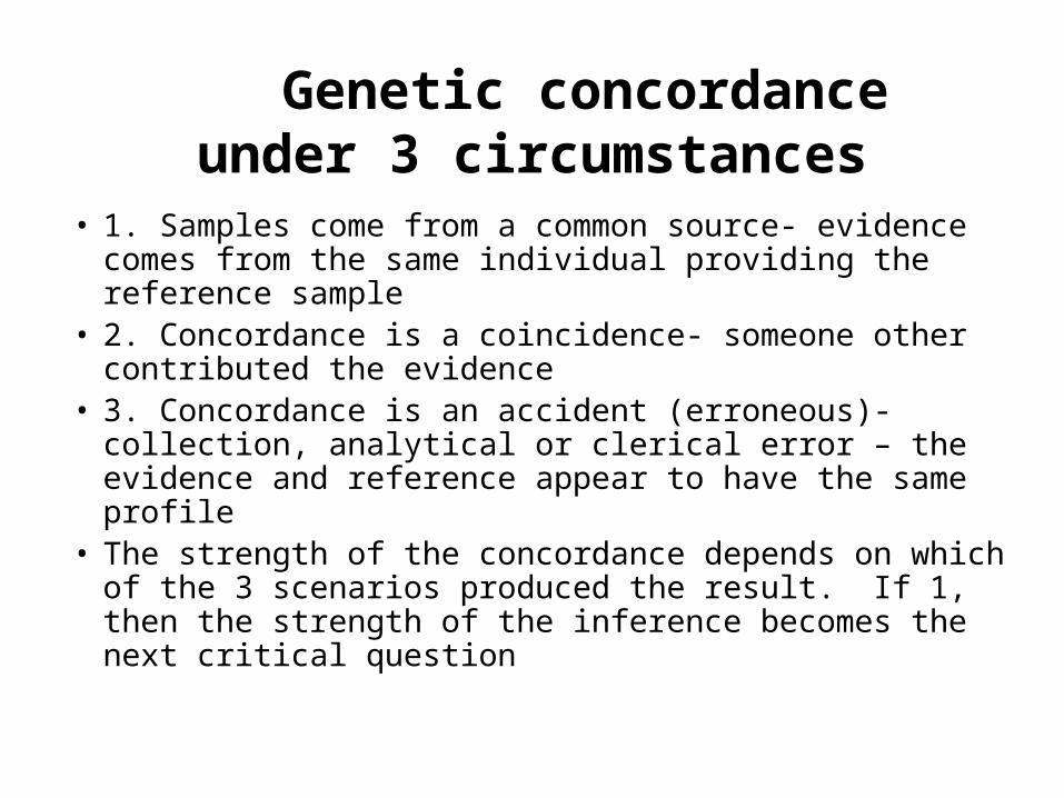
Genetic concordance under 3 circumstances

• 1. Samples come from a common source- evidence comes from the same individual providing the reference sample

• 2. Concordance is a coincidence- someone other contributed the evidence

• 3. Concordance is an accident (erroneous)- collection, analytical or clerical error – the evidence and reference appear to have the same profile

• The strength of the concordance depends on which of the 3 scenarios produced the result. If 1, then the strength of the inference becomes the next critical question

AA

A

A

a

a Aa

aA

aa

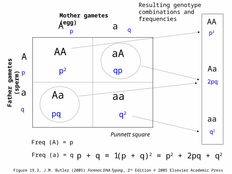
Freq (A) = p

Freq (a) = q (p + q)2 = p2 + 2pq + q2

Punnett square

p2 qp

pq q2

p

q

p q

Fat

her

gam

etes

(sp

erm

)Mother gametes (egg)

p + q = 1

Resulting genotype combinations and frequencies

AA

Aa

p2

2pq

aa

q2

Figure 19.3, J.M. Butler (2005) Forensic DNA Typing, 2nd Edition © 2005 Elsevier Academic Press

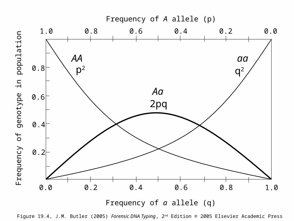
AA aa

Aa

1.0

Frequency of a allele (q)

Frequency of A allele (p)

1.0 0.8 0.6 0.4 0.2 0.0

0.0 0.2 0.4 0.6 0.8

Fre

quen

cy o

f ge

noty

pe in

pop

ulat

ion

0.2

0.4

0.6

0.8 p2

2pq

q2

Figure 19.4, J.M. Butler (2005) Forensic DNA Typing, 2nd Edition © 2005 Elsevier Academic Press

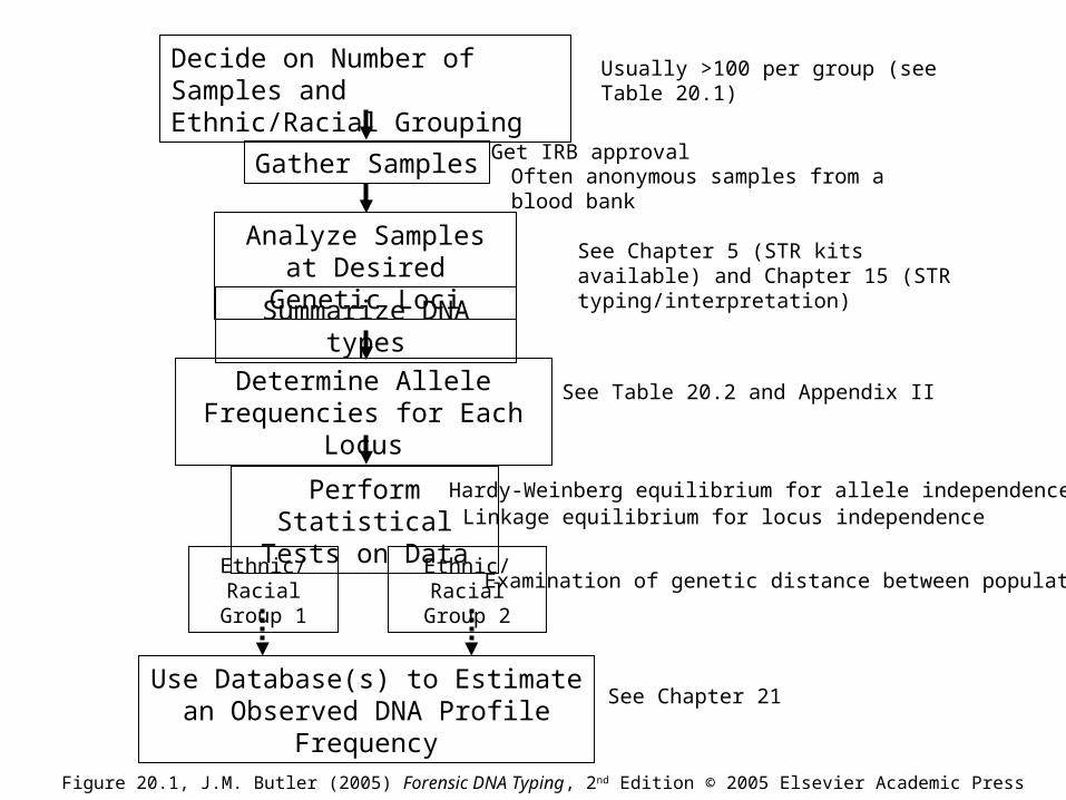
Decide on Number of Samples and Ethnic/Racial Grouping

Gather Samples Get IRB approval

Analyze Samples at Desired Genetic Loci

Summarize DNA types

Ethnic/ Racial Group 1

Ethnic/ Racial Group 2

Determine Allele Frequencies for Each Locus

Perform Statistical Tests on Data

Hardy-Weinberg equilibrium for allele independenceLinkage equilibrium for locus independence

Usually >100 per group (see Table 20.1)

Use Database(s) to Estimate an Observed DNA Profile Frequency

See Chapter 21

Often anonymous samples from a blood bank

See Table 20.2 and Appendix II

See Chapter 5 (STR kits available) and Chapter 15 (STR typing/interpretation)

Examination of genetic distance between populations

Figure 20.1, J.M. Butler (2005) Forensic DNA Typing, 2nd Edition © 2005 Elsevier Academic Press

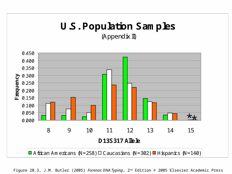
U.S. Population Samples(Appendix II)

0.000

0.050

0.100

0.150

0.200

0.250

0.300

0.350

0.400

0.450

8 9 10 11 12 13 14 15

D13S317 Allele

Fre

qu

ency

African Americans (N=258) Caucasians (N=302) Hispanics (N=140)

**

Figure 20.3, J.M. Butler (2005) Forensic DNA Typing, 2nd Edition © 2005 Elsevier Academic Press

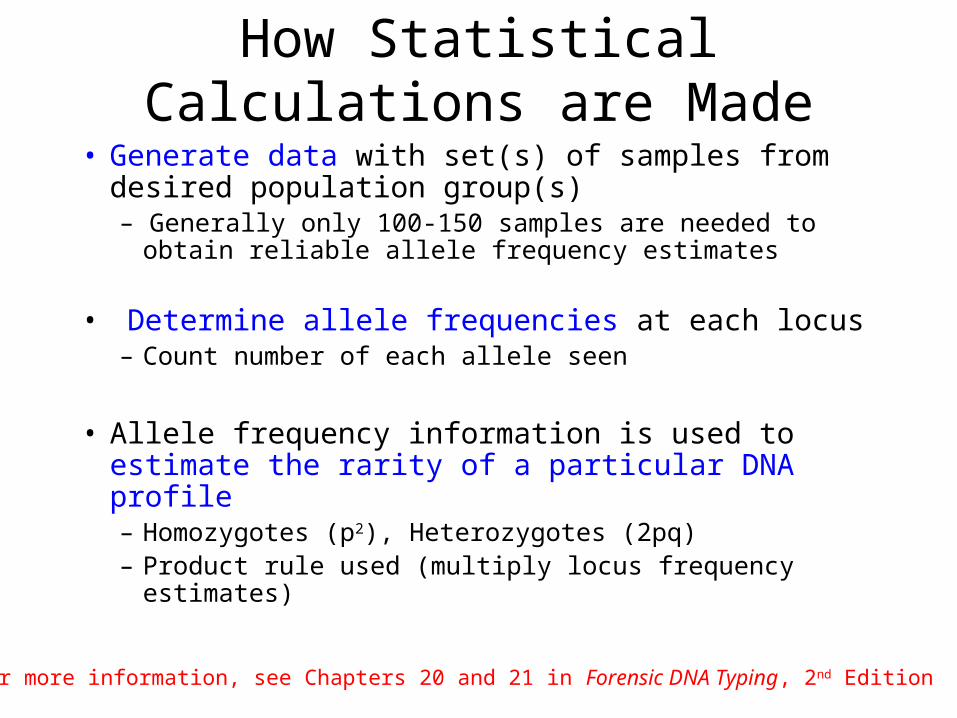
How Statistical Calculations are Made

• Generate data with set(s) of samples from desired population group(s) – Generally only 100-150 samples are needed to obtain

reliable allele frequency estimates

• Determine allele frequencies at each locus– Count number of each allele seen

• Allele frequency information is used to estimate the rarity of a particular DNA profile– Homozygotes (p2), Heterozygotes (2pq)– Product rule used (multiply locus frequency estimates)

For more information, see Chapters 20 and 21 in Forensic DNA Typing, 2nd Edition

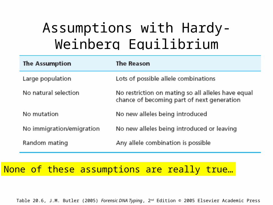
Assumptions with Hardy-Weinberg Equilibrium

None of these assumptions are really true…

Table 20.6, J.M. Butler (2005) Forensic DNA Typing, 2nd Edition © 2005 Elsevier Academic Press

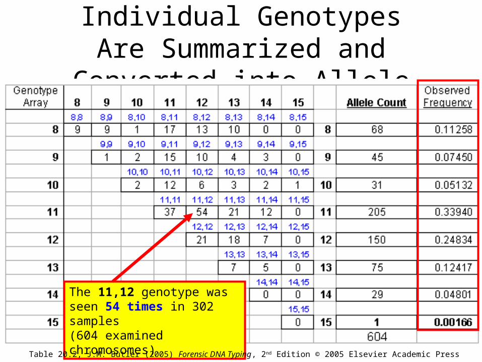
Individual Genotypes Are Summarized and Converted into

Allele Frequencies

The 11,12 genotype was seen 54 times in 302 samples (604 examined chromosomes)

Table 20.2, J.M. Butler (2005) Forensic DNA Typing, 2nd Edition © 2005 Elsevier Academic Press

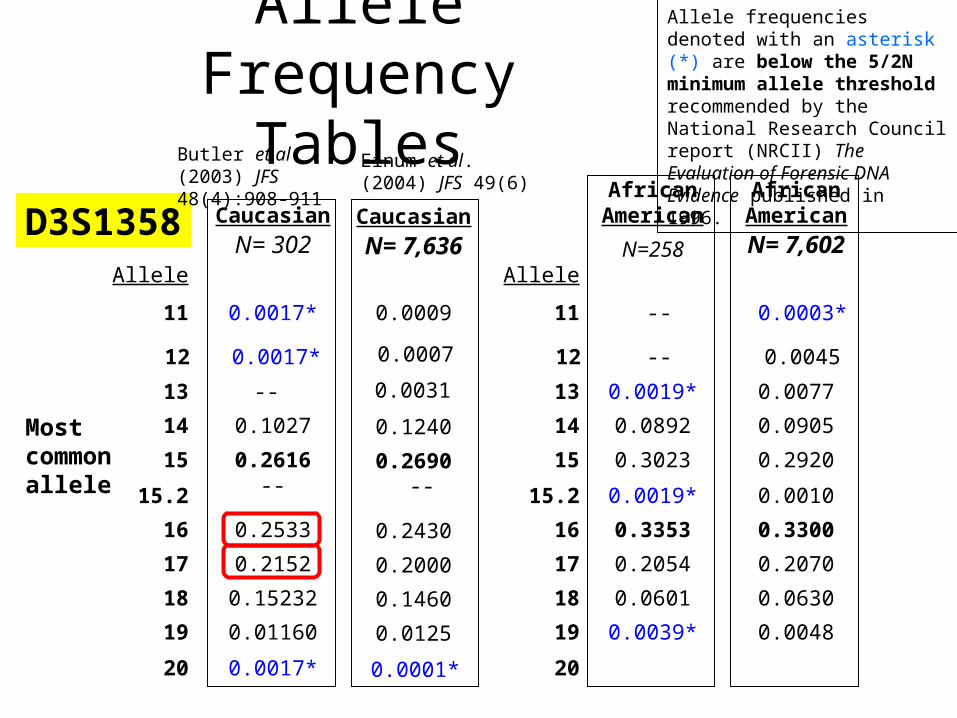
Allele Frequency Tables

  Caucasian

N= 302

 0.0017*

-- 

0.1027

0.2616--

0.2533

0.2152

0.15232

0.01160

African American

N=258

  --

0.0019*

0.0892

0.3023

0.0019*

0.3353

0.2054

0.0601

0.0039*

20 0.0017*  0.0001*  

D3S1358

Butler et al. (2003) JFS 48(4):908-911

Allele frequencies denoted with an asterisk (*) are below the 5/2N minimum allele threshold recommended by the National Research Council report (NRCII) The Evaluation of Forensic DNA Evidence published in 1996.

Most common allele

Caucasian

N= 7,636

 0.0009

 

0.1240

0.2690 --

0.2430

0.2000

0.1460

0.0125

Einum et al. (2004) JFS 49(6)

Allele 11

13

14

15

15.2

16

17

18

19

12 0.0017*  --0.0007

0.0031

African American

N= 7,602

  0.0003*

0.0077

0.0905

0.2920

0.0010

0.3300

0.2070

0.0630

0.0048

 

 0.0045

20

Allele 11

13

14

15

15.2

16

17

18

19

12

Hardy Weinberg Equilibrium

• A predictable relationship exists between allele frequencies and genotype frequencies at a single locus. This mathematical relationship allows for the estimation of genotype frequencies in a population even if the genotype has not been seen in an actual population survey

Hardy Weinberg conditions• Large population- several 100 or more• Approximately Random mating• Negligible to No mutation• Negligible to No migration• Negligible to No selection• “Don’t be ridiculous” over long periods this will not hold• Over short periods HWE may apply• Maintenance of constant allele frequencies also means

genetic variability within a population is not blended away over successive generations.

How a mathematician got into biology

• Story from Mange and Mange- 1999• Hardy loved pure math- which he

considered useless but beautiful! Disliked practical applications. This was one of the most significant practical applications of math in history

• Published in Science to avoid letting his pure math colleagues see it!

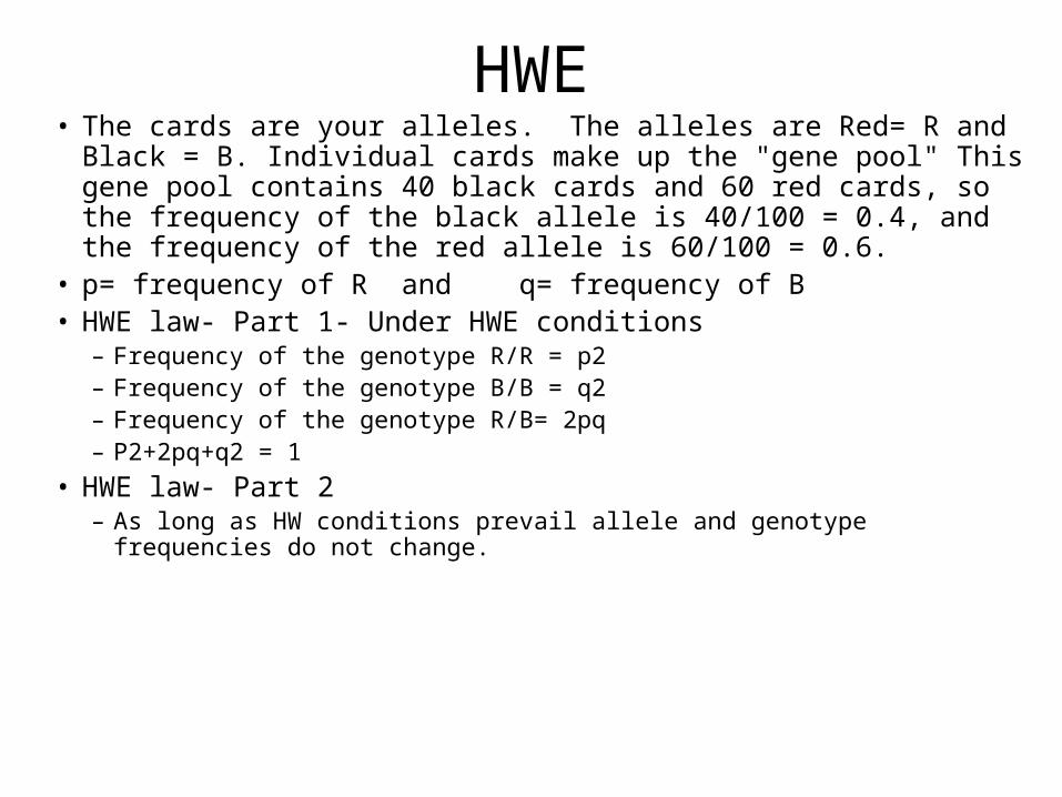
HWE• The cards are your alleles. The alleles are Red= R and Black = B.

Individual cards make up the "gene pool" This gene pool contains 40 black cards and 60 red cards, so the frequency of the black allele is 40/100 = 0.4, and the frequency of the red allele is 60/100 = 0.6.

• p= frequency of R and q= frequency of B • HWE law- Part 1- Under HWE conditions

– Frequency of the genotype R/R = p2– Frequency of the genotype B/B = q2– Frequency of the genotype R/B= 2pq– P2+2pq+q2 = 1

• HWE law- Part 2– As long as HW conditions prevail allele and genotype frequencies do not

change.

HWE simulation

• See handout- We will be mating in class!• Get a pair of cards from the instructor.• In your teams calculate the allele frequencies of R

= red cards and B = black cards• Also tally the genotype frequencies• E.g. number of RR, RB and BB• Team captains provide a summary and write down

the results on the black board

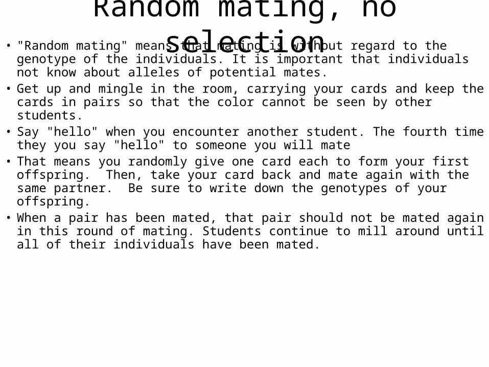
Random mating, no selection• "Random mating" means that mating is without regard to the genotype of the

individuals. It is important that individuals not know about alleles of potential mates.

• Get up and mingle in the room, carrying your cards and keep the cards in pairs so that the color cannot be seen by other students.

• Say "hello" when you encounter another student. The fourth time they you say "hello" to someone you will mate

• That means you randomly give one card each to form your first offspring. Then, take your card back and mate again with the same partner. Be sure to write down the genotypes of your offspring.

• When a pair has been mated, that pair should not be mated again in this round of mating. Students continue to mill around until all of their individuals have been mated.

Tally the results

• In small groups, add up the total number of red cards, black cards and genotypes

• Write down your results on the blackboard.• Did the frequency of the R and B change?• Do the genotypes of the offspring observed

match the genotypes predicted?• Now become your offspring and repeat the

mating and tally.

Random mating- Selection

• Now we will mate with selection. Whenever a RR genotype is formed, this is a lethal combination and results in death.

• Therefore, this combination results in no viable offspring.

• When you mate this time, eliminate any RR genotypes from your tallies.

• Repeat the tally as before

Random mating- Migration

• 5 students will migrate and become geographically isolated

• Mating occurs within two separate populations.

• We will tally results for these 2 populations

• Do you expect the results to be the same as before? Why or why not?