Embed Size (px)
Citation preview
Relation between the geometry of rail welds and thedynamic wheel–rail response: numerical simulationsfor measured weldsM J M M Steenbergen� and C Esveld
Faculty of Civil Engineering and Geosciences, Railway Engineering, Delft University of Technology, Delft, The
Netherlands
The manuscript was received on 8 May 2006 and was accepted after revision for publication on 27 June 2006.
DOI: 10.1243/0954409JRRT87
Abstract: The primary mechanisms playing a role in the dynamic wheel–rail response to railweld irregularities in a ballasted track are pointed out. The concept of P1 and P2 forces for me-tallurgical rail welds, introduced in a first paper [1] concerning the present research, is furtherelaborated. The dynamic wheel–rail response is simulated for a number of geometrical rail weldmeasurements. Results show a good correlation between the gradient of the rail weld geometryand the maximum dynamic wheel–rail contact forces, whereas the correlation with verticalpeak deviations is shown to be very poor. Therefore, an assessment method based on thegradient (introducing a speed-dependent quality index [1]) is more consistent than a methodbased on vertical tolerances. An approximate formula is presented to calculate the maximumdynamic wheel–rail contact force as a function of the train velocity and the maximum gradientof the weld geometry, in analogy to Jenkins’ formulae for calculating P1 and P2 forces at dippedrail joints.
Keywords: rail welds, welding, weld geometry, rail joints, dynamic wheel–rail forces
1 INTRODUCTION
The lifetime of rails in continuously welded rail(CWR) tracks is often determined by the welds,which form the weakest spots in the rail. This isdue to several reasons. First, their vertical geometryis worse than the initial geometry of the rest of therail, leading to local dynamic amplifications of thewheel–rail contact force. Further, the cross-sectionis not constant along the rail (especially for in situmade thermit welds), causing stress concentrationsthat lead to crack initiation and propagation andfinally to failure (especially in the area with tensilestresses). These effects are amplified by the factthat the rail material is inhomogeneous in the longi-tudinal direction because of the difference between
the parent and the weld material and the possibleinclusion of contaminations. Here, also the heat-affected zone and the resulting hardness profile ofthe rail surface play a role. Finally, the residualstress state in the welded rail in combination withthe axial tensile stresses as a result of changing ambi-ent temperatures during winter may lead to earlydamage.
The fatigue crack growth in a welded rail underthe influence of residual stresses was studied bySkyttebol et al. [2]. In this study, it was also foundthat typical crack sizes in welds can lead to failurein a relatively short time if the residual stress fieldinteracts with the axle load. This is the case ifdynamic amplifications of the axle load occurbecause of a bad geometry of the weld. Mutton andAlvarez [3] studied the failure modes in aluminother-mic (thermit) welds under high axle load conditionsand also carried out some experimental investi-gations into the relation between the longitudinalweld profile, the dynamic load amplification factor(DAF), and the train speed.
�Corresponding author: Faculty of Civil Engineering and
Geosciences, Railway Engineering, Delft University of
Technology, Section of Road and Railway Engineering, PO
Box 5048, NL 2600 GA Delft, The Netherlands. email: m.j.m.m.
409
JRRT87 # IMechE 2006 Proc. IMechE Vol. 220 Part F: J. Rail and Rapid Transit
For the reasons explained earlier, the lifetime ofrails in CWR tracks can be significantly extendedby adopting an adequate assessment method forthe welds. Steenbergen and Esveld [1] presented atheoretical model to estimate the maximumdynamic wheel–rail contact forces occurring atthe rail welding surface irregularities. Further, onthe basis of this model, an assessment method forvertical rail weld geometry was presented, basedon the limitation of the gradient of the discretemeasurement signal. The weld quality index (QI)has been introduced as the ratio of the maximumabsolute value of the gradient (on 25 mm basis)of an actual weld measurement to the speed-dependent norm value. It was shown that a linearrelationship between the dynamic wheel–rail forceand the QI exists in theory. Given the fact that therate of track deterioration is determined by thelevel of dynamic contact forces, a weld assessmentbased on the QI is consistent in a life-cycleapproach.
The aim of this article is to validate the modeland the theory presented in reference [1] with thehelp of numerical simulations of the dynamicwheel–rail contact force. In order to perform thisvalidation, the vertical geometry along the rail of239 rail welds has been measured, after which thedynamic wheel–rail response was calculated foreach of them.
2 MODEL FOR SIMULATION OF DYNAMICWHEEL–RAIL INTERACTION AT RAIL WELDS
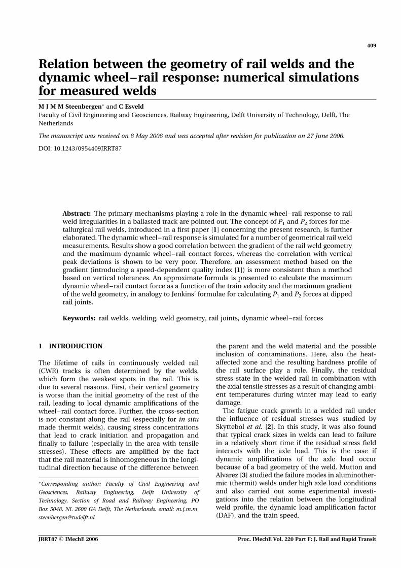
The simulations have been performed with the FE-package DARTS-NL [4]. An overview of the model isgiven in Fig. 1.
The measured irregularity has a sampling intervalof 5 mm and a total length of 1 m. In the model, therail is divided into beam elements with a length of10 mm; therefore, each element has three verticalcoordinates. The irregularity is centred in themiddle of a sleeper span, where the weld is madein practice. The model uses a non-linear Hertziancontact model. The time step in the calculations istaken as the ratio of the element size to the trainvelocity (a reduction of this time step by 50 percent leads to deviations in the results within amargin of 3 per cent). A large number of sleeperbays are included, with non-reflective boundariesat both ends. The number of sleeper bays is, how-ever, not very relevant, given the local effect of theweld irregularity.
3 PRIMARY MECHANISMS IN THE DYNAMICWHEEL–RAIL RESPONSE TO RAIL WELDIRREGULARITIES AND THEIR RELATIONTO TRACK DETERIORATION
In reference [1], the concept of P1 and P2 forces formetallurgical rail welds was introduced, in analogyto the terminology for bolted joints or insulatedrail joints (non-welded joints). It was shown thatthe P1 force, which has, in general, a relativelyhigh frequency, can be attributed to the quasi-instantaneous reaction of the track to the irregular-ity, whereas the P2 force with a relatively lowfrequency can be attributed to the delayed reactionof the axle, which has a much larger inertia relativeto the track.
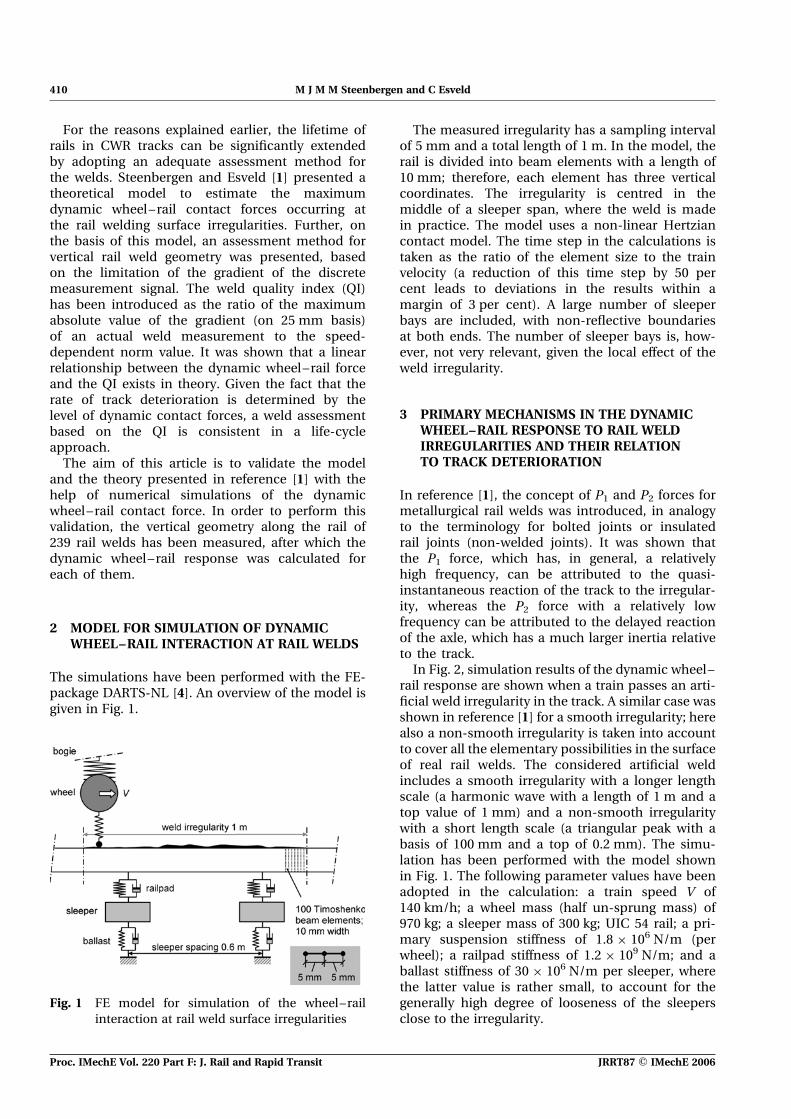
In Fig. 2, simulation results of the dynamic wheel–rail response are shown when a train passes an arti-ficial weld irregularity in the track. A similar case wasshown in reference [1] for a smooth irregularity; herealso a non-smooth irregularity is taken into accountto cover all the elementary possibilities in the surfaceof real rail welds. The considered artificial weldincludes a smooth irregularity with a longer lengthscale (a harmonic wave with a length of 1 m and atop value of 1 mm) and a non-smooth irregularitywith a short length scale (a triangular peak with abasis of 100 mm and a top of 0.2 mm). The simu-lation has been performed with the model shownin Fig. 1. The following parameter values have beenadopted in the calculation: a train speed V of140 km/h; a wheel mass (half un-sprung mass) of970 kg; a sleeper mass of 300 kg; UIC 54 rail; a pri-mary suspension stiffness of 1.8 � 106 N/m (perwheel); a railpad stiffness of 1.2 � 109 N/m; and aballast stiffness of 30 � 106 N/m per sleeper, wherethe latter value is rather small, to account for thegenerally high degree of looseness of the sleepersclose to the irregularity.
Fig. 1 FE model for simulation of the wheel–rail
interaction at rail weld surface irregularities
410 M J M M Steenbergen and C Esveld
Proc. IMechE Vol. 220 Part F: J. Rail and Rapid Transit JRRT87 # IMechE 2006
In Fig. 2, the following quantities are shown as afunction of time:
(a) the geometry of the irregularity z;(b) the dynamic part of the vertical wheel displace-
ment uwheel of the first wheel of a passingbogie, defined positive in the upward directionand calculated in a convective reference framemoving along with the wheel;
(c) the dynamic part of the displacement utrack,dyn ofthe rail/track, calculated in a fixed coordinatesystem with its origin at the centre of the irregu-larity and defined positive in the downwarddirection;
(d) the wheel–rail contact force Fdyn for theconcerned wheel (the dynamic force is
superimposed on the static value), in a convec-tive reference frame;
(e) the axle box acceleration aaxle, in a convectivereference frame;
(f) the dynamic part of the bending moment in therail Mrail,dyn, in a fixed coordinate system at thecentre of the irregularity.
From Fig. 2, a number of observations can be made.They are as follows.
1. The track follows the vertical irregularity quasi-instantaneously; especially for the short-lengthirregularity, this is clearly visible. The wheel dis-placement shows a delay in response relative tothe track. It does not show any influence of theshort peak in the irregularity, whereas this peak
Fig. 2 Dynamic response of the wheel–rail system to an artificial weld with both long and short
length scale irregularities
Geometry of rail welds and the dynamic wheel–rail response 411
JRRT87 # IMechE 2006 Proc. IMechE Vol. 220 Part F: J. Rail and Rapid Transit
is reproduced almost exactly in the raildisplacements.
2. The maximum dynamic contact force is deter-mined by the irregularity with the shortestlength scale. However, the corresponding forcepeaks are rather narrow and the correspondingamount of energy is rather small. These high-frequency peak forces damage mostly the railitself (causing fatigue), as can be seen also in thegraph of the dynamic bending rail moments.The related energy will vanish by wave propa-gation in the rail and by dissipation in, mainly,the railpads.
3. The highest energy of the dynamic contact force iscontained in the ‘carrier frequency’, which can beclearly observed. This carrier frequency is relatedto the delayed reaction of the wheel mass to theirregularity (the P2 force). The relatively largeenergy contained in the relatively low carrier fre-quency is mainly responsible for ballast beddeterioration, as it is not efficiently dissipated inthe rail and the railpads.
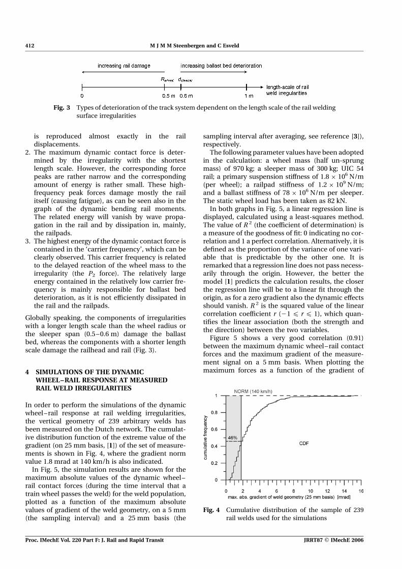
Globally speaking, the components of irregularitieswith a longer length scale than the wheel radius orthe sleeper span (0.5–0.6 m) damage the ballastbed, whereas the components with a shorter lengthscale damage the railhead and rail (Fig. 3).
4 SIMULATIONS OF THE DYNAMICWHEEL–RAIL RESPONSE AT MEASUREDRAIL WELD IRREGULARITIES
In order to perform the simulations of the dynamicwheel–rail response at rail welding irregularities,the vertical geometry of 239 arbitrary welds hasbeen measured on the Dutch network. The cumulat-ive distribution function of the extreme value of thegradient (on 25 mm basis, [1]) of the set of measure-ments is shown in Fig. 4, where the gradient normvalue 1.8 mrad at 140 km/h is also indicated.
In Fig. 5, the simulation results are shown for themaximum absolute values of the dynamic wheel–rail contact forces (during the time interval that atrain wheel passes the weld) for the weld population,plotted as a function of the maximum absolutevalues of gradient of the weld geometry, on a 5 mm(the sampling interval) and a 25 mm basis (the
sampling interval after averaging, see reference [3]),respectively.
The following parameter values have been adoptedin the calculation: a wheel mass (half un-sprungmass) of 970 kg; a sleeper mass of 300 kg; UIC 54rail; a primary suspension stiffness of 1.8 � 106 N/m(per wheel); a railpad stiffness of 1.2 � 109 N/m;and a ballast stiffness of 78 � 106 N/m per sleeper.The static wheel load has been taken as 82 kN.
In both graphs in Fig. 5, a linear regression line isdisplayed, calculated using a least-squares method.The value of R 2 (the coefficient of determination) isa measure of the goodness of fit: 0 indicating no cor-relation and 1 a perfect correlation. Alternatively, it isdefined as the proportion of the variance of one vari-able that is predictable by the other one. It isremarked that a regression line does not pass necess-arily through the origin. However, the better themodel [1] predicts the calculation results, the closerthe regression line will be to a linear fit through theorigin, as for a zero gradient also the dynamic effectsshould vanish. R 2 is the squared value of the linearcorrelation coefficient r (21 4 r 4 1), which quan-tifies the linear association (both the strength andthe direction) between the two variables.
Figure 5 shows a very good correlation (0.91)between the maximum dynamic wheel–rail contactforces and the maximum gradient of the measure-ment signal on a 5 mm basis. When plotting themaximum forces as a function of the gradient of
Fig. 3 Types of deterioration of the track system dependent on the length scale of the rail welding
surface irregularities
Fig. 4 Cumulative distribution of the sample of 239
rail welds used for the simulations
412 M J M M Steenbergen and C Esveld
Proc. IMechE Vol. 220 Part F: J. Rail and Rapid Transit JRRT87 # IMechE 2006
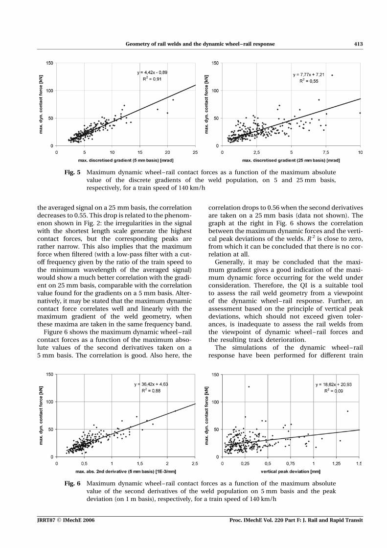
the averaged signal on a 25 mm basis, the correlationdecreases to 0.55. This drop is related to the phenom-enon shown in Fig. 2: the irregularities in the signalwith the shortest length scale generate the highestcontact forces, but the corresponding peaks arerather narrow. This also implies that the maximumforce when filtered (with a low-pass filter with a cut-off frequency given by the ratio of the train speed tothe minimum wavelength of the averaged signal)would show a much better correlation with the gradi-ent on 25 mm basis, comparable with the correlationvalue found for the gradients on a 5 mm basis. Alter-natively, it may be stated that the maximum dynamiccontact force correlates well and linearly with themaximum gradient of the weld geometry, whenthese maxima are taken in the same frequency band.
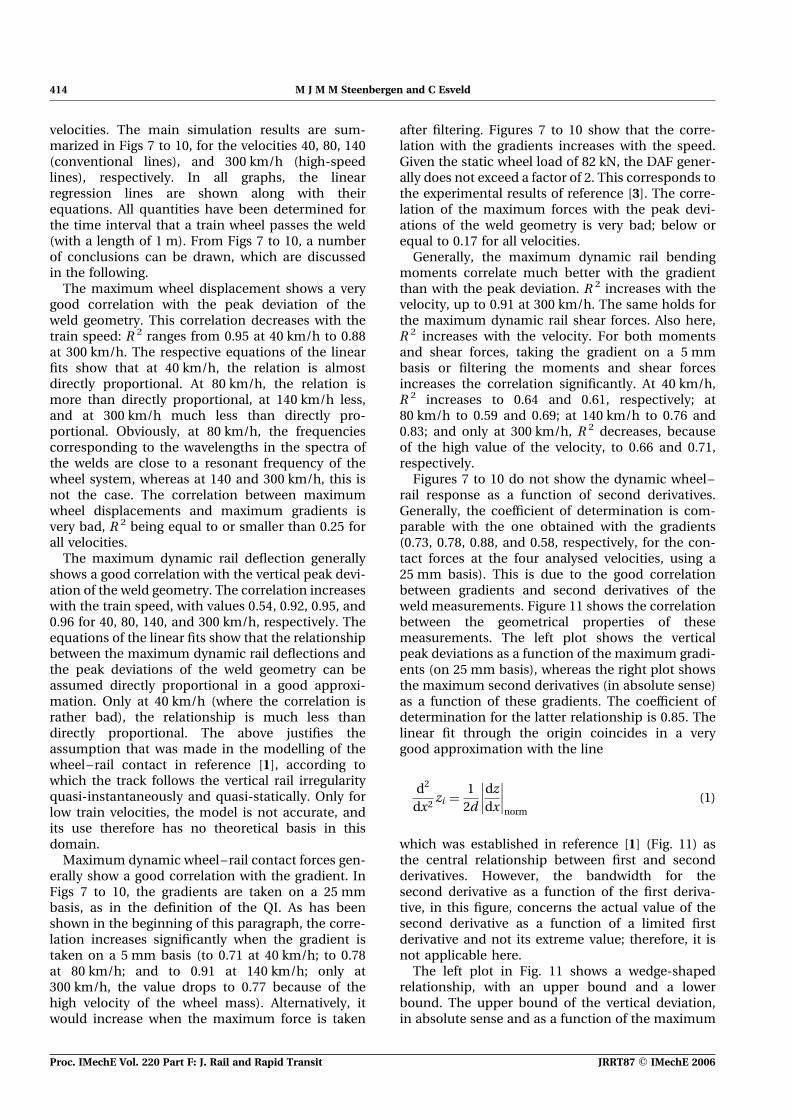
Figure 6 shows the maximum dynamic wheel–railcontact forces as a function of the maximum abso-lute values of the second derivatives taken on a5 mm basis. The correlation is good. Also here, the
correlation drops to 0.56 when the second derivativesare taken on a 25 mm basis (data not shown). Thegraph at the right in Fig. 6 shows the correlationbetween the maximum dynamic forces and the verti-cal peak deviations of the welds. R 2 is close to zero,from which it can be concluded that there is no cor-relation at all.
Generally, it may be concluded that the maxi-mum gradient gives a good indication of the maxi-mum dynamic force occurring for the weld underconsideration. Therefore, the QI is a suitable toolto assess the rail weld geometry from a viewpointof the dynamic wheel–rail response. Further, anassessment based on the principle of vertical peakdeviations, which should not exceed given toler-ances, is inadequate to assess the rail welds fromthe viewpoint of dynamic wheel–rail forces andthe resulting track deterioration.
The simulations of the dynamic wheel–railresponse have been performed for different train
Fig. 6 Maximum dynamic wheel–rail contact forces as a function of the maximum absolute
value of the second derivatives of the weld population on 5 mm basis and the peak
deviation (on 1 m basis), respectively, for a train speed of 140 km/h
Fig. 5 Maximum dynamic wheel–rail contact forces as a function of the maximum absolute
value of the discrete gradients of the weld population, on 5 and 25 mm basis,
respectively, for a train speed of 140 km/h
Geometry of rail welds and the dynamic wheel–rail response 413
JRRT87 # IMechE 2006 Proc. IMechE Vol. 220 Part F: J. Rail and Rapid Transit
velocities. The main simulation results are sum-marized in Figs 7 to 10, for the velocities 40, 80, 140(conventional lines), and 300 km/h (high-speedlines), respectively. In all graphs, the linearregression lines are shown along with theirequations. All quantities have been determined forthe time interval that a train wheel passes the weld(with a length of 1 m). From Figs 7 to 10, a numberof conclusions can be drawn, which are discussedin the following.
The maximum wheel displacement shows a verygood correlation with the peak deviation of theweld geometry. This correlation decreases with thetrain speed: R 2 ranges from 0.95 at 40 km/h to 0.88at 300 km/h. The respective equations of the linearfits show that at 40 km/h, the relation is almostdirectly proportional. At 80 km/h, the relation ismore than directly proportional, at 140 km/h less,and at 300 km/h much less than directly pro-portional. Obviously, at 80 km/h, the frequenciescorresponding to the wavelengths in the spectra ofthe welds are close to a resonant frequency of thewheel system, whereas at 140 and 300 km/h, this isnot the case. The correlation between maximumwheel displacements and maximum gradients isvery bad, R 2 being equal to or smaller than 0.25 forall velocities.
The maximum dynamic rail deflection generallyshows a good correlation with the vertical peak devi-ation of the weld geometry. The correlation increaseswith the train speed, with values 0.54, 0.92, 0.95, and0.96 for 40, 80, 140, and 300 km/h, respectively. Theequations of the linear fits show that the relationshipbetween the maximum dynamic rail deflections andthe peak deviations of the weld geometry can beassumed directly proportional in a good approxi-mation. Only at 40 km/h (where the correlation israther bad), the relationship is much less thandirectly proportional. The above justifies theassumption that was made in the modelling of thewheel–rail contact in reference [1], according towhich the track follows the vertical rail irregularityquasi-instantaneously and quasi-statically. Only forlow train velocities, the model is not accurate, andits use therefore has no theoretical basis in thisdomain.
Maximum dynamic wheel–rail contact forces gen-erally show a good correlation with the gradient. InFigs 7 to 10, the gradients are taken on a 25 mmbasis, as in the definition of the QI. As has beenshown in the beginning of this paragraph, the corre-lation increases significantly when the gradient istaken on a 5 mm basis (to 0.71 at 40 km/h; to 0.78at 80 km/h; and to 0.91 at 140 km/h; only at300 km/h, the value drops to 0.77 because of thehigh velocity of the wheel mass). Alternatively, itwould increase when the maximum force is taken
after filtering. Figures 7 to 10 show that the corre-lation with the gradients increases with the speed.Given the static wheel load of 82 kN, the DAF gener-ally does not exceed a factor of 2. This corresponds tothe experimental results of reference [3]. The corre-lation of the maximum forces with the peak devi-ations of the weld geometry is very bad; below orequal to 0.17 for all velocities.
Generally, the maximum dynamic rail bendingmoments correlate much better with the gradientthan with the peak deviation. R 2 increases with thevelocity, up to 0.91 at 300 km/h. The same holds forthe maximum dynamic rail shear forces. Also here,R 2 increases with the velocity. For both momentsand shear forces, taking the gradient on a 5 mmbasis or filtering the moments and shear forcesincreases the correlation significantly. At 40 km/h,R 2 increases to 0.64 and 0.61, respectively; at80 km/h to 0.59 and 0.69; at 140 km/h to 0.76 and0.83; and only at 300 km/h, R 2 decreases, becauseof the high value of the velocity, to 0.66 and 0.71,respectively.
Figures 7 to 10 do not show the dynamic wheel–rail response as a function of second derivatives.Generally, the coefficient of determination is com-parable with the one obtained with the gradients(0.73, 0.78, 0.88, and 0.58, respectively, for the con-tact forces at the four analysed velocities, using a25 mm basis). This is due to the good correlationbetween gradients and second derivatives of theweld measurements. Figure 11 shows the correlationbetween the geometrical properties of thesemeasurements. The left plot shows the verticalpeak deviations as a function of the maximum gradi-ents (on 25 mm basis), whereas the right plot showsthe maximum second derivatives (in absolute sense)as a function of these gradients. The coefficient ofdetermination for the latter relationship is 0.85. Thelinear fit through the origin coincides in a verygood approximation with the line
d2
dx2zi ¼ 1
2d
dz
dx
����
����norm
(1)
which was established in reference [1] (Fig. 11) asthe central relationship between first and secondderivatives. However, the bandwidth for thesecond derivative as a function of the first deriva-tive, in this figure, concerns the actual value of thesecond derivative as a function of a limited firstderivative and not its extreme value; therefore, it isnot applicable here.
The left plot in Fig. 11 shows a wedge-shapedrelationship, with an upper bound and a lowerbound. The upper bound of the vertical deviation,in absolute sense and as a function of the maximum
414 M J M M Steenbergen and C Esveld
Proc. IMechE Vol. 220 Part F: J. Rail and Rapid Transit JRRT87 # IMechE 2006
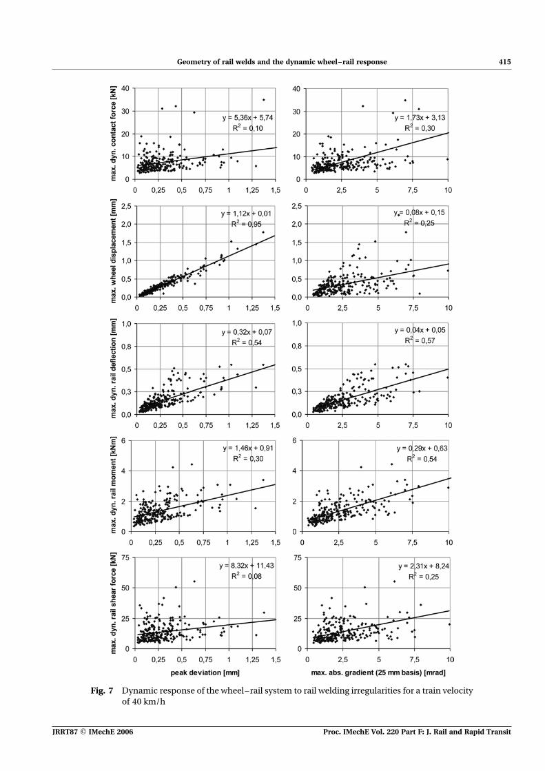
Fig. 7 Dynamic response of the wheel–rail system to rail welding irregularities for a train velocity
of 40 km/h
Geometry of rail welds and the dynamic wheel–rail response 415
JRRT87 # IMechE 2006 Proc. IMechE Vol. 220 Part F: J. Rail and Rapid Transit
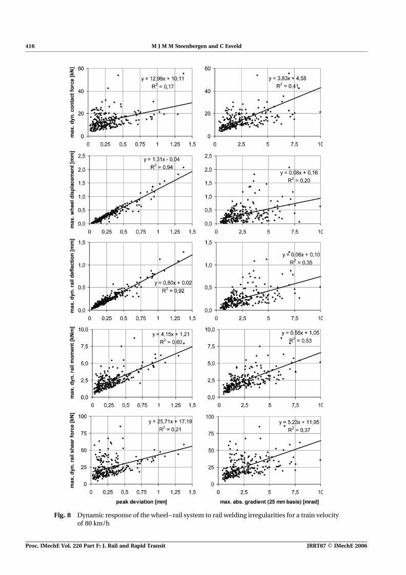
Fig. 8 Dynamic response of the wheel–rail system to rail welding irregularities for a train velocity
of 80 km/h
416 M J M M Steenbergen and C Esveld
Proc. IMechE Vol. 220 Part F: J. Rail and Rapid Transit JRRT87 # IMechE 2006
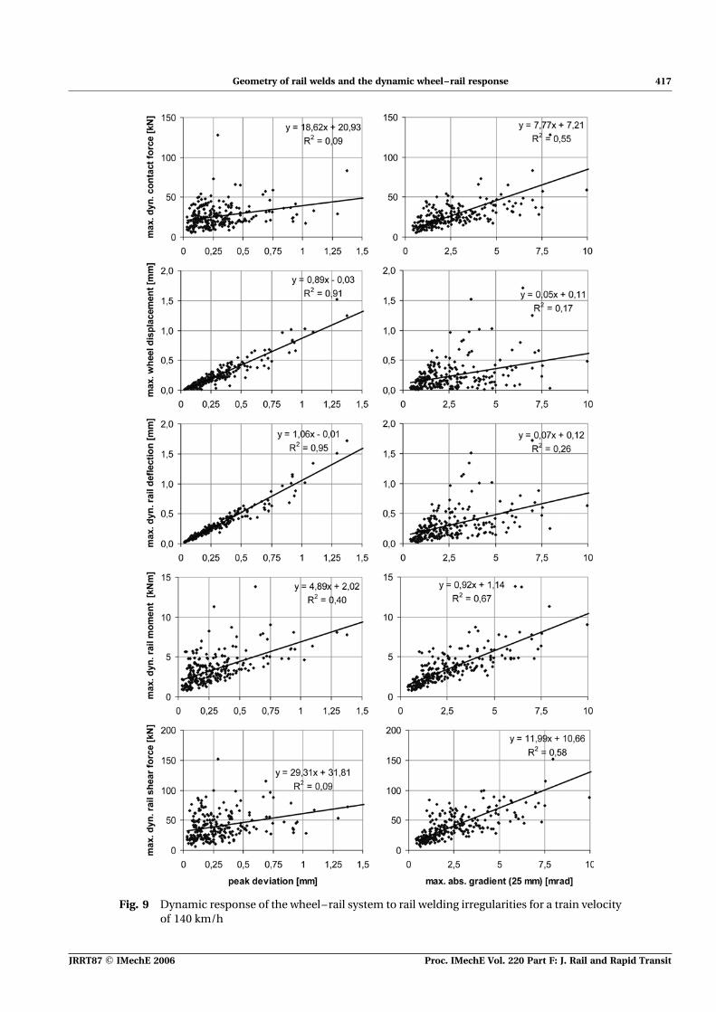
Fig. 9 Dynamic response of the wheel–rail system to rail welding irregularities for a train velocity
of 140 km/h
Geometry of rail welds and the dynamic wheel–rail response 417
JRRT87 # IMechE 2006 Proc. IMechE Vol. 220 Part F: J. Rail and Rapid Transit
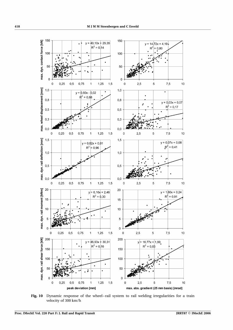
Fig. 10 Dynamic response of the wheel–rail system to rail welding irregularities for a train
velocity of 300 km/h
418 M J M M Steenbergen and C Esveld
Proc. IMechE Vol. 220 Part F: J. Rail and Rapid Transit JRRT87 # IMechE 2006

value of the discretized gradient, is given by (seereference [1], Fig. 12)
zmax ¼ 14Lmax
dz
dx
����
����max
, Lmax ¼ 2000 mm (2)
The lower bound is given by
zmin ¼ 14Lmin
dz
dx
����
����max
, Lmin ¼ 100 mm (3)
The exceptional excess of some values withrespect to the lower boundary is due to the filteringand averaging processes of the original sampledsignal, as pointed out in reference [1]. The wedge-shaped relationship between peak deviations andgradients can be easily recognized in several plotsin Figs 7 to 10.
5 INFLUENCE OF THE VELOCITY ONTHE RELATION BETWEEN FORCES ANDRAIL WELD GRADIENTS
In reference [1], the following relationship has beenderived theoretically
Fdyn,max ¼ gMtrackV2 1
d
dz
dx
����
����max
(4)
where g(–) is a dimensionless calibration factor(dependent on the line section speed interval);Mtrack(kg) the equivalent track mass; V(m/s) thetrain speed; d(m) the sampling distance in the aver-aged and filtered signals of the weld geometry(0.025 m), and jdz/dxjmax (–) the intervention levelfor the gradient of this signal. The linear relationshipbetween the gradient and the maximum dynamiccontact force was confirmed by the analyses in thepreceding section. The focus will now be on therelation between the maximum dynamic contact
Fig. 12 Dependence of the dynamic wheel–rail contact forces at rail welds on the train velocity
Fig. 11 Vertical peak deviations and maximum second derivatives in absolute sense,
respectively, as a function of the maximum gradient in absolute sense of the measured
welds (derivatives on 25 mm basis)
Geometry of rail welds and the dynamic wheel–rail response 419
JRRT87 # IMechE 2006 Proc. IMechE Vol. 220 Part F: J. Rail and Rapid Transit
force and the velocity, which according to equation(4) is quadratic.
In Fig. 12 at the left, the relation between the maxi-mum dynamic wheel–rail contact force and thegradient (on 25 mm basis) is shown for the differentvelocities for which simulations were performed. Foreach velocity, a linear fit through the origin is dis-played (which is not equal to the regression line);the equations of these fits are given by (jdz/dxjmax ¼tan a and Fdyn in kN)
40 km/h: Fdyn ¼ 2:5 tana (5a)
80 km/h: Fdyn ¼ 4:9 tana (5b)
140 km/h: Fdyn ¼ 9:5 tana (5c)
300 km/h: Fdyn ¼ 15:7 tana (5d)
It should be remarked that the graphs in Fig. 12 showlinear fits, disregarding any scatter in the results.Therefore, actual values may exceed the predictedvalues from Fig. 12, especially at low velocities (seeFigs 7 to 10).
Figure 12 shows, at the right, the relation betweenthe contact force and the train speed, given a certaingradient, which is taken as 5 mrad. It is observed thatthe influence of the velocity is not quadratic, as ispredicted from equation (4). However, in general,the relation between the force and the speed canbe well approximated as linear, yielding the followingadapted relationship (4)
Fdyn,max ¼ gMtrackV1
d
dz
dx
����
����max
(6)
The linear relationship between the maximumdynamic contact force (or the DAF) and the trainspeed is confirmed experimentally by the results ofreference [3]. The linear relationship (6) betweenforce, speed, and gradient allows combiningequations (5) into the following approximate singleequation, in terms of the variables V(m/s) andjdz/dxjmax (¼tan a) (mrad)
Fdyn,max ¼ 0:22 � V � tana (kN) (7)
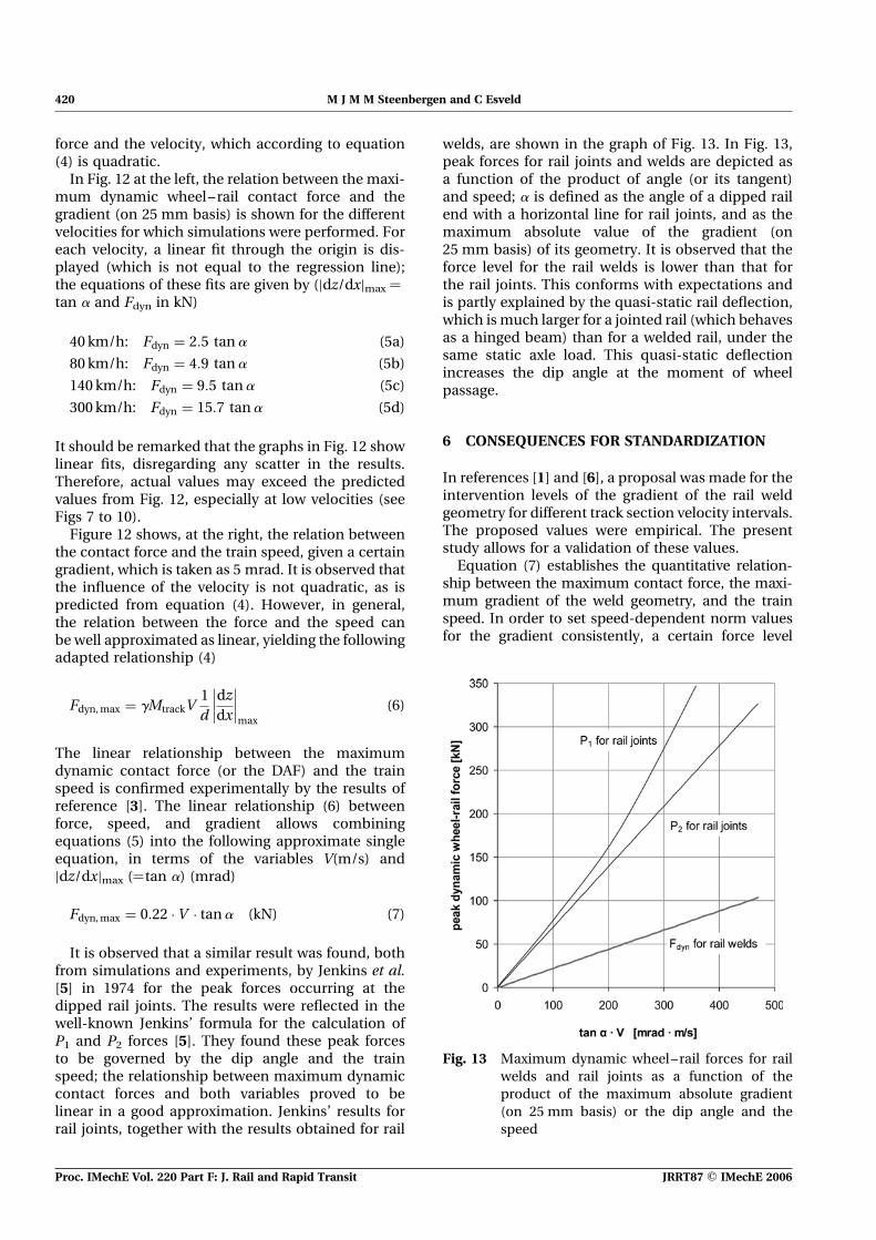
It is observed that a similar result was found, bothfrom simulations and experiments, by Jenkins et al.[5] in 1974 for the peak forces occurring at thedipped rail joints. The results were reflected in thewell-known Jenkins’ formula for the calculation ofP1 and P2 forces [5]. They found these peak forcesto be governed by the dip angle and the trainspeed; the relationship between maximum dynamiccontact forces and both variables proved to belinear in a good approximation. Jenkins’ results forrail joints, together with the results obtained for rail
welds, are shown in the graph of Fig. 13. In Fig. 13,peak forces for rail joints and welds are depicted asa function of the product of angle (or its tangent)and speed; a is defined as the angle of a dipped railend with a horizontal line for rail joints, and as themaximum absolute value of the gradient (on25 mm basis) of its geometry. It is observed that theforce level for the rail welds is lower than that forthe rail joints. This conforms with expectations andis partly explained by the quasi-static rail deflection,which is much larger for a jointed rail (which behavesas a hinged beam) than for a welded rail, under thesame static axle load. This quasi-static deflectionincreases the dip angle at the moment of wheelpassage.
6 CONSEQUENCES FOR STANDARDIZATION
In references [1] and [6], a proposal was made for theintervention levels of the gradient of the rail weldgeometry for different track section velocity intervals.The proposed values were empirical. The presentstudy allows for a validation of these values.
Equation (7) establishes the quantitative relation-ship between the maximum contact force, the maxi-mum gradient of the weld geometry, and the trainspeed. In order to set speed-dependent norm valuesfor the gradient consistently, a certain force level
Fig. 13 Maximum dynamic wheel–rail forces for rail
welds and rail joints as a function of the
product of the maximum absolute gradient
(on 25 mm basis) or the dip angle and the
speed
420 M J M M Steenbergen and C Esveld
Proc. IMechE Vol. 220 Part F: J. Rail and Rapid Transit JRRT87 # IMechE 2006
should be admitted. This level should be coupled withthe level of weld-related track deterioration; however,little is known regarding this relationship. Instead, twofacts may be taken as a point of departure.
1. The empirical tolerance of 0.3 mm has been usedworldwide for several decades, not leading to sys-tematic problems. The maximum peak deviationfollowing from the standardized gradient should,for 140 km/h (which is a regular passenger trainspeed), not be from a different order of magnitude.
2. The quality of the newly manufactured rail, aftertrack laying but before track use, corresponds toa gradient of 0.7 mrad (as has been shown inreference [1]).
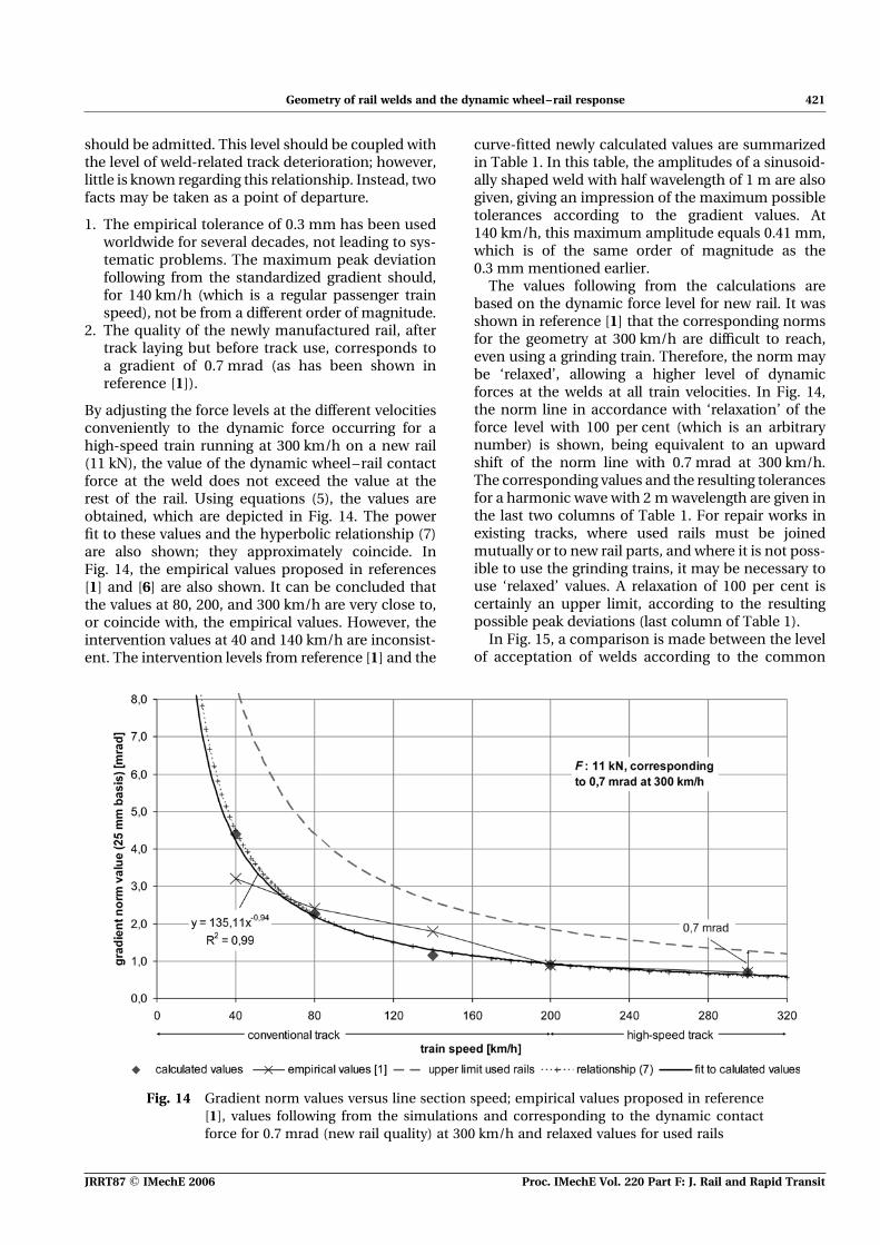
By adjusting the force levels at the different velocitiesconveniently to the dynamic force occurring for ahigh-speed train running at 300 km/h on a new rail(11 kN), the value of the dynamic wheel–rail contactforce at the weld does not exceed the value at therest of the rail. Using equations (5), the values areobtained, which are depicted in Fig. 14. The powerfit to these values and the hyperbolic relationship (7)are also shown; they approximately coincide. InFig. 14, the empirical values proposed in references[1] and [6] are also shown. It can be concluded thatthe values at 80, 200, and 300 km/h are very close to,or coincide with, the empirical values. However, theintervention values at 40 and 140 km/h are inconsist-ent. The intervention levels from reference [1] and the
curve-fitted newly calculated values are summarizedin Table 1. In this table, the amplitudes of a sinusoid-ally shaped weld with half wavelength of 1 m are alsogiven, giving an impression of the maximum possibletolerances according to the gradient values. At140 km/h, this maximum amplitude equals 0.41 mm,which is of the same order of magnitude as the0.3 mm mentioned earlier.
The values following from the calculations arebased on the dynamic force level for new rail. It wasshown in reference [1] that the corresponding normsfor the geometry at 300 km/h are difficult to reach,even using a grinding train. Therefore, the norm maybe ‘relaxed’, allowing a higher level of dynamicforces at the welds at all train velocities. In Fig. 14,the norm line in accordance with ‘relaxation’ of theforce level with 100 per cent (which is an arbitrarynumber) is shown, being equivalent to an upwardshift of the norm line with 0.7 mrad at 300 km/h.The corresponding values and the resulting tolerancesfor a harmonic wave with 2 mwavelength are given inthe last two columns of Table 1. For repair works inexisting tracks, where used rails must be joinedmutually or to new rail parts, and where it is not poss-ible to use the grinding trains, it may be necessary touse ‘relaxed’ values. A relaxation of 100 per cent iscertainly an upper limit, according to the resultingpossible peak deviations (last column of Table 1).
In Fig. 15, a comparison is made between the levelof acceptation of welds according to the common
Fig. 14 Gradient norm values versus line section speed; empirical values proposed in reference
[1], values following from the simulations and corresponding to the dynamic contact
force for 0.7 mrad (new rail quality) at 300 km/h and relaxed values for used rails
Geometry of rail welds and the dynamic wheel–rail response 421
JRRT87 # IMechE 2006 Proc. IMechE Vol. 220 Part F: J. Rail and Rapid Transit
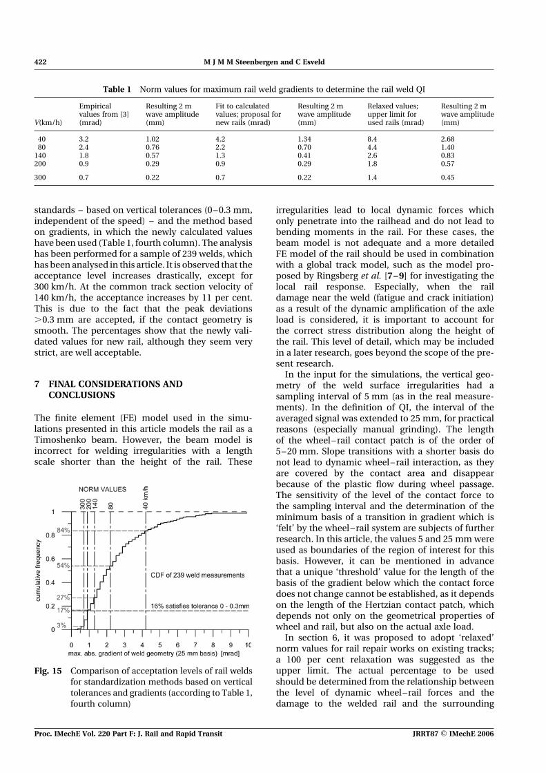
standards – based on vertical tolerances (0–0.3 mm,independent of the speed) – and the method basedon gradients, in which the newly calculated valueshave been used (Table 1, fourth column). The analysishas been performed for a sample of 239 welds, whichhas been analysed in this article. It is observed that theacceptance level increases drastically, except for300 km/h. At the common track section velocity of140 km/h, the acceptance increases by 11 per cent.This is due to the fact that the peak deviations.0.3 mm are accepted, if the contact geometry issmooth. The percentages show that the newly vali-dated values for new rail, although they seem verystrict, are well acceptable.
7 FINAL CONSIDERATIONS ANDCONCLUSIONS
The finite element (FE) model used in the simu-lations presented in this article models the rail as aTimoshenko beam. However, the beam model isincorrect for welding irregularities with a lengthscale shorter than the height of the rail. These
irregularities lead to local dynamic forces whichonly penetrate into the railhead and do not lead tobending moments in the rail. For these cases, thebeam model is not adequate and a more detailedFE model of the rail should be used in combinationwith a global track model, such as the model pro-posed by Ringsberg et al. [7–9] for investigating thelocal rail response. Especially, when the raildamage near the weld (fatigue and crack initiation)as a result of the dynamic amplification of the axleload is considered, it is important to account forthe correct stress distribution along the height ofthe rail. This level of detail, which may be includedin a later research, goes beyond the scope of the pre-sent research.
In the input for the simulations, the vertical geo-metry of the weld surface irregularities had asampling interval of 5 mm (as in the real measure-ments). In the definition of QI, the interval of theaveraged signal was extended to 25 mm, for practicalreasons (especially manual grinding). The lengthof the wheel–rail contact patch is of the order of5–20 mm. Slope transitions with a shorter basis donot lead to dynamic wheel–rail interaction, as theyare covered by the contact area and disappearbecause of the plastic flow during wheel passage.The sensitivity of the level of the contact force tothe sampling interval and the determination of theminimum basis of a transition in gradient which is‘felt’ by the wheel–rail system are subjects of furtherresearch. In this article, the values 5 and 25 mmwereused as boundaries of the region of interest for thisbasis. However, it can be mentioned in advancethat a unique ‘threshold’ value for the length of thebasis of the gradient below which the contact forcedoes not change cannot be established, as it dependson the length of the Hertzian contact patch, whichdepends not only on the geometrical properties ofwheel and rail, but also on the actual axle load.
In section 6, it was proposed to adopt ‘relaxed’norm values for rail repair works on existing tracks;a 100 per cent relaxation was suggested as theupper limit. The actual percentage to be usedshould be determined from the relationship betweenthe level of dynamic wheel–rail forces and thedamage to the welded rail and the surrounding
Fig. 15 Comparison of acceptation levels of rail welds
for standardization methods based on vertical
tolerances and gradients (according to Table 1,
fourth column)
Table 1 Norm values for maximum rail weld gradients to determine the rail weld QI
V(km/h)
Empiricalvalues from [3](mrad)
Resulting 2 mwave amplitude(mm)
Fit to calculatedvalues; proposal fornew rails (mrad)
Resulting 2 mwave amplitude(mm)
Relaxed values;upper limit forused rails (mrad)
Resulting 2 mwave amplitude(mm)
40 3.2 1.02 4.2 1.34 8.4 2.6880 2.4 0.76 2.2 0.70 4.4 1.40140 1.8 0.57 1.3 0.41 2.6 0.83200 0.9 0.29 0.9 0.29 1.8 0.57
300 0.7 0.22 0.7 0.22 1.4 0.45
422 M J M M Steenbergen and C Esveld
Proc. IMechE Vol. 220 Part F: J. Rail and Rapid Transit JRRT87 # IMechE 2006
track. Further, the norm values were derived assum-ing a constant static axle load, whereas different axleloads of different train/track typesmay have an influ-ence. These are subjects for further research, boththeoretically and experimentally.
From this study, which considered the dynamicwheel–rail response to rail weld surface irregularitieson a ballasted track, a number of conclusions can bedrawn. They are as follows.
1. During the train wheel passage, the track followsa vertical rail weld surface irregularity quasi-instantaneously, whereas the wheel displacementshows a delay in response relative to the track.This phenomenon causes P1 and P2 wheel–railforces.
2. The maximum dynamic contact force is deter-mined by the irregularity with the shortest lengthscale. However, the corresponding force peaks arerather narrow and the corresponding amount ofenergy is rather small; these high-frequency peakforces damage mostly the rail itself.
3. The delayed reaction of the wheel mass results ina carrier frequency in the contact force. The high-est amount of energy of the dynamic contact forceis contained in this relatively low frequency. Therelatively large energy contained in this carrier fre-quency is mainly responsible for the ballast beddeterioration, as it is not efficiently dissipated inthe rail and the railpads.
4. There is no correlation between the maximumdynamic wheel–rail forces and the peak deviationof the vertical weld geometry. Therefore, anassessment based on the principle of peak devi-ations satisfying tolerances is inadequate toassess the geometry of rail welds from the view-point of dynamic wheel–rail forces and the result-ing track deterioration.
5. The maximum gradient of the vertical weld geo-metry gives a good indication of the maximumdynamic wheel–rail forces occurring for a trainwheel passing the weld. Therefore, the QI is a suit-able tool to assess the rail weld geometry from aviewpoint of the dynamic wheel–rail response.
6. An approximate formula is derived, relating themaximum dynamic wheel–rail contact force at aweld irregularity linearly to the maximum gradi-ent of the weld geometry and the train velocity.A similar (quasi-)linear relation between peakforces, train velocity, and dip angle has beenestablished by Jenkins et al. for rail joints.
7. Normvalues for thegradient of the longitudinal geo-metry of aweld have beenderived depending on theline section train speed, allowing to determine theQI to assess the geometry of a rail weld [1]. Thesenorm values lead to a uniform level of dynamiccontact forces for all running speeds.
The present research is continued with an exper-imental study, in which the wheel–rail contactforces are measured for different types of weldingirregularities and passing trains on real track. Pre-liminary test results were presented in reference [10].
ACKNOWLEDGEMENTS
The FE simulations, results of which have been pre-sented in this article, have been carried out byJorge Rivero Granero, in the framework of the Eras-mus student exchange program between the DelftUniversity of Technology and the Technical Univer-sity of Catalonia (Barcelona). The present researchwas performed in assignment of the Dutch RailInfra Manager ProRail. Rolf Dollevoet (ProRail) isacknowledged for his kind permission to publishthe research results presented in this article.
REFERENCES
1 Steenbergen, M. J. M. M. and Esveld, C. Relationbetween the geometry of rail welds and the dynamicwheel–rail response: numerical simulations formeasured welds. Proc. IMechE, Part F: J. Rail andRapid Transit, 2006, 220(F4), 409–423. (This paper.)
2 Skyttebol, A., Josefson, B. L., and Ringsberg, J. W. Fati-gue crack growth in a welded rail under the influence ofresidual stresses. Eng. Fract. Mech., 2005, 72, 271–285.
3 Mutton, P. J. and Alvarez, E. F. Failure modes in alumi-nothermic rail welds under high axle load conditions.Eng. Fail. Anal., 2004, 11, 151–166.
4 DARTS-NL. Dynamic analysis of a rail track structure,2006, available from www.esveld.com.
5 Jenkins, H. H., Stephenson, J., Clayton, G. A.,Morland, G. W., and Lyon, D. The effect of track andvehicle parameters on wheel/rail vertical dynamicforces. Rail. Eng. J., January 1974, 2–16.
6 Steenbergen, M. J. M. M., Esveld, C., and Dollevoet,R. P. B. J. New Dutch assessment of rail welding geo-metry. Eur. Rail. Rev., 2005, 11, 71–79.
7 Ringsberg, J. W., Bjarnehed, H., Johansson, A., andJosefson, B. L. Rolling contact fatigue of rails–finiteelement modelling of residual stresses, strains andcrack initiation. Proc. Instn Mech. Engrs, Part F: J. Railand Rapid Transit, 2000, 214, 7–19.
8 Ringsberg, J. W. and Josefson, B. L. Finite element ana-lyses of rolling contact fatigue crack initiation in rail-heads. Proc. Instn Mech. Engrs, Part F: J. Rail andRapid Transit, 2001, 215, 243–259.
9 Ringsberg, J. W. and Lindback, T. Rolling contact fati-gue analysis of rails including numerical simulations ofthe rail manufacturing process and repeated wheel–railcontact loads. Int. J. Fatigue, 2003, 25, 547–558.
10 Esveld, C. and Steenbergen, M. J. M. M. Force-basedassessment of rail welds. In Proceedings of 7th WorldCongress on Railway research, Montreal, Canada, 4–8June 2006.
Geometry of rail welds and the dynamic wheel–rail response 423
JRRT87 # IMechE 2006 Proc. IMechE Vol. 220 Part F: J. Rail and Rapid Transit