JSS Journal of Statistical SoftwareMMMMMM YYYY, Volume VV, Issue II. http://www.jstatsoft.org/

spTimer: Spatio-Temporal Bayesian Modeling Using

R

K.S. Bakar

Yale University, USAS.K. Sahu

University of Southampton, UK

Abstract

Hierarchical Bayesian modeling of large point referenced space-time data is increasinglybecoming feasible in many environmental applications due to the recent advances in bothstatistical methodology and computation power. Implementation of these methods usingthe Markov chain Monte Carlo (MCMC) computational techniques, however, requiresdevelopment of problem specific and user written computer code, possibly in a low levellanguage. This programming requirement is hindering the widespread use of the Bayesianmodel based analysis methods among practitioners and, hence there is an urgent need todevelop high level software packages that can analyze large data sets rich in both spaceand time.

This paper develops the package spTimer for hierarchical Bayesian modeling of stylizedenvironmental space-time monitoring data as a contributed software package in the R

language that is fast becoming a very popular statistical computing platform. The packageis able to fit, spatially and temporally predict large amounts of space-time data usingthree recently developed Bayesian models. The user is given control over many optionsregarding covariance function selection, distance calculation, prior selection and tuningof the implemented MCMC algorithms, although suitable defaults are provided. Thepackage has many other attractive features such as on the fly transformations and anability to spatially predict temporally aggregated summaries on the original scale, whichsaves the problem of storage when using MCMC methods for large datasets. A simulationexample, with more than a million observations, and a real life data example are used tovalidate the underlying code and to illustrate the software capabilities.

Keywords: Bayesian spatio-temporal modeling, Markov chain Monte Carlo, Gibbs sampling,autoregressive, predictive processes.

1. Introduction

Model based Bayesian analysis methods are becoming popular for taking account of uncer-

2 spTimer: Spatio-Temporal Bayesian Modeling Using R

tainties in the analysis and spatial and temporal prediction of environmental space-time data.Practitioners are increasingly benefiting from their ability to reduce uncertainty in the infer-ence statements that arise from joint space-time modeling (Cressie and Wikle 2011). Bayesianmethods are also popular because of their ability to combine information from several sourcesusing melding or data fusion (Sahu, Gelfand, and Holland 2010). However, currently thereis no suitable software package for Bayesian modeling and analysis of large space-time data.In this paper, our interest is on modeling and analyzing spatio-temporal point referenceddata (Banerjee, Carlin, and Gelfand 2004), where random observations are measured overtime at a number of spatial locations, which vary continuously over a study region.

A number of R (R Development Core Team 2006) packages are available for modeling and ana-lyzing spatial data, e.g., the packages sp (Pebesma and Bivand 2005) and spacetime (Pebesma2012; Bivand, Pebesma, and Gomez-Rubio 2013). Furthermore, packages gstat (Pebesma2004), splm (Millo and Piras 2012), fields (Furrer, Nychka, and Sain 2013) and nlme

(Pinheiro, Bates, DebRoy, and Sarkar 2013) are able to fit spatial regression models and per-form spatial interpolation based on Kriging (Krige 1951). Some packages are also availablefor analyzing spatial point pattern data (Banerjee et al. 2004), see e.g., spatial (Ripley 2013;Venables and Ripley 2002) and spatstat (Baddeley and Turner 2005). However, none of thesepackages implement MCMC based Bayesian modeling methods.

General purpose R software packages, such as MCMCpack (Martin, Quinn, and Park 2011),MCMCglmm (Hadfield 2010), and BLR (Campos and Rodriguez 2012), are available for im-plementing Bayesian models. However, these are not suitable for analyzing spatially correlateddata. Packages that can handle spatial correlations include spBayes (Finley and Banerjee2013), geoR (Ribeiro and Diggle 2001), geoRglm (Christensen and Ribeiro 2002), rjags(Plummer 2014) and R2WinBUGS (Sturtz, Ligges, and Gelman 2005) which is an R interfaceto WinBUGS (Spiegelhalter, Thomas, and Best 1999). However, these are not suitable andsometimes complicated for modeling data rich in both space and time, although the packagespBayes can model spatially varying short-length time series data. These packages are notintended to handle large, e.g., more than a million, space-time data and these packages do notallow incorporation of popular models in the time series literature such as the auto-regressivemodels.

Non-Bayesian packages implementing the generalized additive models such as gam (Hastie2013) and mgcv (Wood 2013) can also fit models for spatial data by implementing functionalrelationships between the response and the coordinates of the spatial locations, e.g., latitudeand longitude. However, these modeling approaches are not process based, i.e., do not incor-porate random spatial and temporal processes, and we find that our process based modelsimplemented in spTimer have superior performance in out of sample spatial predictions, seeSections 4 and 5.

The main contribution of this paper is the development of the R package spTimer that isavailable from the Comprehensive R Archive Network (CRAN). The package enables Bayesianmodeling of regularly monitored point referenced data obtained from a sparse spatial networkof monitoring stations. Data at each monitoring station are obtained as a regular time seriesbut may contain missing data. The package is also able to incorporate an arbitrary numberof explanatory variables that may vary in both space and time. The residual spatio-temporalvariation is modeled using three different recently developed modeling methods appropriatefor analyzing space-time environmental monitoring data. All the inferences in this packageand the paper are proposed to be under the Bayesian paradigm using MCMC methods.

Journal of Statistical Software 3

Using Bayesian computation methods, the package spTimer is able to process, i.e., fit andpredict, both spatially and temporally, large space-time data sets that may contain missingdata. In so doing, the user is able to choose a particular covariance function from the Maternfamily (Cressie 1993) for the underlying Gaussian process and also a suitable method for calcu-lating distances between two locations. In addition, the user can select the hyper-parametersof the prior distributions and is also given the ability to choose the tuning parameters for theimplemented MCMC algorithms. The package also allows the user to select one of the twopossible (log and square-root) on the fly transformations for the response variable. Anotherattractive feature of the package is the ability to spatially predict temporally aggregated sum-maries, e.g., annual mean from daily data, on the original scale, which only requires storageof the annual aggregate, instead of the full length time series, for each prediction location ateach MCMC iteration when we fit and predict for large data sets.

Users of spTimer only need to provide the model specifications in the high level R language,but the main body of the code is developed using the C programming language, that ishidden from the user. This enables faster computation and better data handling capacitythan what can be achieved by simply using R. However, once the MCMC iterations havebeen finished the output can be analyzed using any other contributed R package such ascoda (Plummer, Best, Cowles, and Vines 2006). For model selection purposes, the packageautomatically reports the values of a predictive model selection criteria (Gelfand and Ghosh1998). Many other utility functions for model validation and output analyzes are also pro-vided. The main functions of the package spTimer are discussed in detail in Section 3.

The first of the three models (see Section 2) implemented in spTimer is a hierarchical nuggeteffect model together with an independent Gaussian process (GP) model at each time point.The Gaussian process implies a spatio-temporal random effect that captures the space-timeinteractions, see e.g., Cressie and Wikle (2011, Chapter 6). Overall, this model parallels thespatial random effect model in spatial only data analysis and naturally provides a very simplestarting model in many investigations involving space-time data, see Banerjee et al. (2004);Diggle and Ribeiro (2007); and Gelfand, Diggle, Fuentes, and Guttorp (2010).

The second implemented model is the hierarchical auto-regressive model for space-time datadeveloped by Sahu, Gelfand, and Holland (2007). An explicit auto-regressive term for theunderlying true spatio-temporal process is assumed in a hierarchical set-up that includes theoverall nugget effect. This model is included in the spTimer package because of its supe-rior performance in modeling air-pollution data, see e.g., Cameletti, Ignaccolo, and Bande(2009) and Sahu and Bakar (2012a). This auto-regressive (AR) model is modified, as thethird and final implemented model, to include the recently developed Gaussian predictiveprocess approximation technique for handling large spatial and spatio-temporal data follow-ing Banerjee, Gelfand, Finley, and Sang (2008), Finley, Sang, Banerjee, and Gelfand (2009)and Sahu and Bakar (2012b). This last paper illustrates the capability of spTimer in han-dling and processing more than a million space-time observations within a reasonable amountof computing time in a standard personal computer.

This paper illustrates the package spTimer with two examples. The first is a simulationexample (see Section 4) that is used for code verification and illustration of the softwarecapabilities. The highlight of this example is that it simulates more than a million space-timeobservations from the third model based on a Gaussian predictive process approximation. Itthen fits the model and illustrates prediction using MCMC methods. The code for the othertwo models are verified using a smaller simulation data set. A real data example, modeling

4 spTimer: Spatio-Temporal Bayesian Modeling Using R

the daily 8-hour maximum ozone concentration in the months of July and August 2006 in thestate of New York, is used for rapid illustration of the models and methods, see Section 5.

2. Spatio-temporal models

2.1. Preliminaries

The Bayesian spatio-temporal models can be represented in a hierarchical structure, where,according to Gelfand (2012), we specify distributions for data, process and parameters inthree stages:

First [data|process, parameter]

Second [process|parameter]

Third [parameter]

In the second stage, the process can add different levels, for example in Gaussian Process(GP) models (Cressie and Wikle 2011; Gelfand et al. 2010) we have true underlying processin the first level and the spatio-temporal random effect in the second level of the hierarchy.Some illustrations are provided below in Section 2.2. Further examples, based on temporalprocesses, are given in Sections 2.3 and 2.4. In the third stage of the hierarchy we introducethe prior distribution of the parameters or hyper-parameters.

The models are described for time series data that are segmented using two different unitsof time, such as hours within days or days within years, to have extra flexibility in modelingand inputting data into the package. This enables us, for example, to model observed ozoneconcentration levels during the high ozone season (May to September in the United States)in each year for several years without having to model data for the remaining months ineach year when ozone concentration levels are low and not harmful (Sahu and Bakar 2012b).However, by default, the package works for modeling data indexed by just one unit of time.

Let l and t denote the two units of time where l denotes the longer unit, e.g., year, l = 1, . . . , r,and t denotes the shorter unit, e.g., day, t = 1, . . . , Tl where r and Tl denote the total numberof two time units, respectively. Let Zl(si, t) denote the observed point referenced data andOl(si, t) be the true value corresponding to Zl(si, t) at site si, i = 1, ..., n at time denotedby two indices l and t. Let Zlt = (Zl(s1, t), ..., Zl(sn, t))

′ and Olt = (Ol(s1, t), ..., Ol(sn, t))′.

We shall denote all the observed data by z and z∗ will denote all the missing data. Let

N = n∑r

l=1 Tl be the total number of observations to be modeled.

Throughout, the notation ǫlt = (ǫl(s1, t), ..., ǫl(sn, t))′ will be used to denote the so called

nugget effect or the pure error term assumed to be independently normally distributedN(0, σ2

ǫ In), where σ2ǫ is the unknown pure error variance and In is the identity matrix of

order n. The spatio-temporal random effects will be denoted by ηlt = (ηl(s1, t), ..., ηl(sn, t))′

and these will be assumed to follow N(0,Ση) independently in time, where Ση = σ2ηSη, σ

2η

is the site invariant spatial variance and Sη is the spatial correlation matrix obtained fromthe, often used, general Matern correlation function (Matern 1986; Handcock and Stein 1993;Handcock and Wallis 1994) defined as:

κ(si, sj ;φ, ν) =1

2ν−1Γ(ν)(2√ν||si − sj ||φ)νKν(2

√ν||si − sj ||φ), φ > 0, ν > 0, (1)

Journal of Statistical Software 5

where Γ(ν) is the standard gamma function, Kν is the modified Bessel function of second kindwith order ν, and ||si − sj || is the distance between sites si and sj . The parameter φ controlsthe rate of decay of the correlation as the distance ||si − sj || increases and the parameter νcontrols smoothness of the random field (Banerjee et al. 2004; Cressie 1993). The packagespTimer allows several possibilities regarding estimation of the correlation parameters φ andν that range from fixing them (point mass prior) to estimating them by assuming suitableprior distributions, see Section 2.5 for further details. In addition, spTimer is also able toincorporate the spherical correlation function, see Banerjee et al. (2004).

In the development below, we assume that there are p covariates, including the intercept,denoted by the n× p matrix Xlt. Some of these covariates may vary in space and time. Thenotation β = (β1, ..., βp) will be used to denote the p× 1 vector of regression coefficients. Weshall use the generic notation θ to denote all the parameters.

2.2. GP model specification

The independent Gaussian process (GP) model is specified hierarchically by:

Zlt = Olt + ǫlt, (2)

Olt = Xltβ + ηlt, (3)

for each l = 1, . . . , r and t = 1, . . . , Tl, where we assume that ǫlt and ηlt are independent andeach are normally distributed with their respective parameters as given in Section 2.1. LetO denote all the random effects, Olt, l = 1, . . . , r and t = 1, . . . , Tl. Let θ = (β, σ2

ǫ , σ2η, φ, ν)

denote all the parameters of this model and let π(θ) denote the prior distribution that weshall specify later. The logarithm of the joint posterior distribution of the parameters andthe missing data for this GP model is given by:

log π(θ,O, z∗|z) ∝ −N

2log σ2

ǫ −1

2σ2ǫ

r∑

l=1

Tl∑

t=1

(Zlt −Olt)′(Zlt −Olt)−

∑rl=1 Tl

2log |σ2

η Sη|

− 1

2σ2η

r∑

l=1

Tl∑

t=1

(Olt −Xltβ)′S−1

η (Olt −Xltβ) + log π(θ). (4)

The prior distribution π(θ) is specified in Section 2.5 and the full conditional distributions ofthe parameters, required for Gibbs sampling, are provided in Appendix A.

2.3. AR model specification

Following Sahu et al. (2007), we specify the hierarchical AR models as follows:

Zlt = Olt + ǫlt, (5)

Olt = ρOlt−1 +Xltβ + ηlt, (6)

for all l and t; where, ρ denotes the unknown temporal correlation parameter assumed tobe in the interval (−1, 1). Obviously, for ρ = 0, these models reduce to the GP modelsdescribed above in Section 2.2. We continue to assume the Gaussian distributions, introducedin Section 2.1, for ǫlt and ηlt for all values of l and t.

The auto-regressive models require specification of the initial term Ol0 for each l = 1, . . . , r.Here we specify an independent spatial model for each Ol0 with mean µl and the covariance

6 spTimer: Spatio-Temporal Bayesian Modeling Using R

matrix σ2l S0 where the correlation matrix S0 is obtained using the Matern correlation function

in Equation (1) with the same set of correlation parameters φ and ν for ηlt.

Let θ denote all the parameters, i.e., θ = (β, ρ, σ2ǫ , σ

2η, φ, ν,µl, σ

2l ) and we also suppose that

O contains all the parameters Olt for l = 1, . . . , r, t = 0, . . . , Tl. The logarithm of the jointposterior distribution of the parameters and the missing data is now given by:

log π(θ,O, z∗|z) ∝ −N

2log σ2

ǫ −1

2σ2ǫ

r∑

l=1

Tl∑

t=1

(Zlt −Olt)′(Zlt −Olt)−

∑rl=1 Tl

2log |σ2

η Sη|

− 1

2σ2η

r∑

l=1

Tl∑

t=1

(Olt − ρOlt−1 −Xltβ)′S−1

η (Olt − ρOlt−1 −Xltβ)

−1

2

r∑

l=1

log |σ2l S0| −

1

2

r∑

l=1

1

σ2l

(Ol0 − µl)′S−1

0 (Ol0 − µl) + log π(θ). (7)

As for the GP models of previous section, the prior distributions are specified in Section 2.5.Full conditional distributions are provided in Appendix B.

2.4. Spatio-temporal models based on GPP

These models are based on the recent work by Sahu and Bakar (2012b) and the main idea hereis to define the random effects ηl(si, t) at a smaller number, m, of locations, called the knots,and then use kriging to predict those random effects at the data and prediction locations.Here, an AR model is only assumed for the random effects at the knot locations and not forall the random effects at the observation locations. At the top level we assume the model:

Zlt = Xltβ +Awlt + ǫlt, (8)

for all l and t, where A = CS−1η and C denotes the n by m cross-correlation matrix between

the random effects at the n observation locations and m knot locations, s∗1, . . . , s∗

m, and Sη

is the m by m correlation matrix of the m random effects wlt. We specify wlt at the knotsconditionally given wlt−1 as:

wlt = ρwlt−1 + ηlt, (9)

for all l and t, where ηlt ∼ N(0,Ση) independently, Ση = σ2ηSη. Note that, here Ση is an

m×m matrix which is of much lower dimensional than the same for two previous models GPand AR since we assume that m << n.

The auto-regressive models are completed by the assumption for the initial conditions, wl0 ∼N(0, σ2

l S0) independently for each l = 1, . . . , r, where the correlation matrix S0 is obtained byusing the Matern correlation function in Equation (1) with decay parameter φ. Let w denotethe random effects wlt for l = 1, . . . , r and t = 0, 1, . . . , Tl. Let θ denote all the parametersβ, ρ, σ2

ǫ , σ2w, φ, ν, σ

2l , l = 1, ..., r. The logarithm of the joint posterior distribution of the

parameters and the missing data is given by:

log π(θ,w, z∗|z) ∝ −N

2log σ2

ǫ −1

2σ2ǫ

r∑

l=1

Tl∑

t=1

(Zlt −Xltβ −Awlt)′(Zlt −Xltβ −Awlt)

−m∑r

l=1 Tl

2log σ2

η −∑r

l=1 Tl

2log |Sη| −

1

2σ2η

r∑

l=1

Tl∑

t=1

(wlt − ρwlt−1)′S−1

η

Journal of Statistical Software 7

(wlt − ρwlt−1)−m

2

r∑

l=1

log σ2l −

r

2log |S0| −

1

2

r∑

l=1

1

σ2l

wl0S−10 wl0

+ log π(θ). (10)

As previously in Sections 2.2 and 2.3, we specify the prior distributions in Section 2.5. Thefull conditional distributions for Gibbs sampling are provided in Appendix C.

2.5. Prior distributions

The Bayesian model for each of the above three specifications is completed by assumingsuitable prior distributions for the underlying parameters. For simplicity and convenience,we group the model parameters of different spatial processes and data into three differenttypes depending on whether those describe: the mean, the variance or the correlation. Allthe parameters describing the mean, e.g., β, ρ, other than the random effects, are givenindependent normal prior distributions, where the user can specify the means (µβ, µρ) andvariances (δ2β, δ

2ρ). In our illustrations in Section 3, we have taken all those means to be 0

and variances to be 1010, that correspond to our assumption of flat prior distributions. Wealso define an independent normal prior distribution with mean 0 and σ2

µ, assumed to be 1010

in our illustrations, for each component of the n-dimensional vector µl in the autoregressivemodel.

The prior distribution for a typical precision (inverse of variance) parameter is specifiedthrough a gamma distribution with mean a/b and variance a/b2. The user can specify anysuitable values for a and b, but in our illustrations we have chosen a = 2 and b = 1 to have aproper prior distribution for any variance component that will guarantee a proper posteriordistribution (Gelman, Carlin, Stern, and Rubin 2004).

There is a large literature regarding the identifiability and the consistency of the parametersdescribing the correlation in a Gaussian process; see for example, Stein (1999) and Zhang(2004). These problems manifest themselves in the Bayesian estimation literature as well,see e.g., Sahu, Gelfand, and Holland (2006), who use an empirical Bayes (EB) approach. Tofacilitate estimation using this EB approach, spTimer allows the user to run Gibbs samplingby fixing the correlation parameters φ and ν so that a grid search can be performed to findthe optimal values of these parameters.

Full Bayesian estimation of φ and ν is also allowed in spTimer corresponding to discreteuniform prior distributions for both these parameters. In all our illustrations the smoothingparameter ν is estimated using a discrete uniform prior distribution taking values from 0 to1.5 with the increment 0.05. In addition to a discrete uniform distribution, we also allow aGamma prior distribution with suitable hyper-parameter values for the decay parameter φ.

In practice, in any Bayesian analysis, the sensitivity with respect to the chosen distributionmust be studied, and the spTimer package that we have developed here makes it easy to doso without much programming effort.

2.6. Model fitting

All the models are fitted using Gibbs sampling (Gelfand and Smith 1990). The conjugate priordistributions assumed for all the parameters except for the φ and ν enable standard conjugatesampling from the full conditional distributions. These details are given in Appendices A, B,

8 spTimer: Spatio-Temporal Bayesian Modeling Using R

and C. Missing data values are sampled from their conditional distributions at each iterationof the Gibbs sampler.

The full conditional distributions of the correlation parameters φ and ν are non-standard.The package provides two options for sampling these parameters corresponding to the twodifferent prior distributions. The full conditional distribution will be discrete, and henceeasy to sample from, if a discrete uniform prior distribution has been assumed for them. Thesecond option, only allowed for the decay parameter φ, is to assign a continuous uniform priordistribution over an interval or a Gamma prior distribution and then to use the random-walkMetropolis-Hastings algorithm to draw samples from it. The proposal distribution is takenas the normal distribution with the mean at the current value and the variance σ2

p which istuned to have an acceptance rate between 15 to 40%, see Gelman et al. (2004) for theoreticaljustifications. The Metropolis algorithm is implemented on the log-scale for φ, i.e., we workwith the density of log(φ) instead of φ since the support of the normal proposal distributionis the real line. In this sampling scheme, keeping φ within a range, as may be required by theassumed prior distribution, is trivial since any proposal value outside the range is rejectedforthwith.

The quality of the model fit and its predictive abilities are assessed by calculating the predic-tive model choice criteria (PMCC) (Gelfand and Ghosh 1998) which is given by,

PMCC =n∑

i=1

r∑

l=1

Tl∑

t=1

{E(Zl(si, t)rep − zl(si, t))

2 + V ar(Zl(si, t)rep)}, (11)

where, Zl(si, t)rep denotes a future replicate of the data zl(si, t). The first term in the PMCCassesses the goodness of fit and second term is a penalty term for model complexity. ThePMCC, justified using a squared error loss function, is most suitable for comparing Bayesianhierarchical models that involve a first stage Gaussian model. The values of the criteria areestimated by sampling from the posterior predictive distributions discussed below.

2.7. Prediction details

Spatial prediction at a new location and temporal prediction at future time points proceedwith the posterior predictive distribution for Zl(s0, t

′), where s0 denotes a new location and t′

is a time point, which can be in the future. The posterior predictive distribution for Zl(s0, t′)

is obtained by integrating over the parameters with respect to the joint posterior distributionas:

π(Zl(s0, t′)|z) =

∫π(Zl(s0, t

′)|Ol(s0, t′), σ2

ǫ

)× π

(Ol(s0, t

′)|θ,O, z∗)

×π (θ,O, z∗|z) dOl

(s0, t

′)dO dθ dz∗. (12)

Note that for the GPP models in Section 2.4 we replace the random effects Ol(s, t′) by wl(s, t

′).Predictions are obtained by composition sampling. First, a random sample θ(j),O(j) is drawnfrom the posterior distribution π(θ,O, z∗|z) using the details in the model fitting described in

Sections 2.2, 2.3, 2.4. Then, Bayesian kriging is applied to draw a sample, O(j)l (s0, t

′) from the

conditional distribution of Ol(s0, t′) given Ol(s1, t), . . . , Ol(sn, t). Finally a sample Z

(j)l (s0, t

′)

is drawn from the top level model π(Zl(s0, t′)|O(j)

l (s0, t′), σ

2(j)ǫ ).

At the end of the MCMC run, the samples Z(j)l (s0, t

′), j = 1, . . . , J where J is a large number,are summarized to make predictive inference. If a transformation, such as the log or the square

Journal of Statistical Software 9

root, has been applied then the posterior predictive samples Z(j)l (s0, t

′) are first transformedback to the original scale before their summaries are calculated. Further, details regardingthese predictions are provided in Bakar (2012) for the GP models, Sahu et al. (2007) for theAR models and Sahu and Bakar (2012b) for the GPP based models.

3. Main functions in spTimer

There are two main functions in the spTimer package, namely, spT.Gibbs for model fittingand predict to obtain spatial and temporal predictions based on the fitted models. Table 1provides a snapshot of these two main functions. In the following sub-sections we discussthese functions more elaborately.

Function Description

spT.Gibbs For model fitting using Gibbs sampling approach.It can also predict simultaneously if suitable options are turned on.

predict.spT Using output from spT.Gibbs this is able to perform prediction,or predict either spatially or temporally or both.

Table 1: Two main functions in spTimer.

3.1. spT.Gibbs

The function spT.Gibbs is used to fit all three models using the Gibbs sampling approachand it takes a number of arguments that define and control its behavior. For example, theargument formula is used to specify the linear part of the model. It is an object of classformula, which is same as that for the lm function to fit linear regression models in R.

The argument data provides the data frame to be used for model fitting. The package alsohas the capability to support data classes STFDF of spacetime and SpatialPointsDataFrame

of sp. The data set must be first ordered by the location index, and for each location the datamust be ordered by time. Time-series data with more than one segment, for example, Tl unit(e.g., daily) observations in the lth segment (l = 1, . . . , r) (e.g., month), must be ordered firstby the longer unit (e.g., month) and then by the shorter unit (e.g., day). The total lengthof the time series at each location,

∑rl=1 Tl, must be the same for each location and the data

rows in each site must correspond to the same basic time unit.

Varying segment length time series are also allowed, e.g., T1 = 31, T2 = 28, T3 = 31, andT4 = 30 when it is intended to model daily data for the first four calendar months (r = 4) in ayear which is not a leap year. Moreover, all sites must have data rows for the exact same totalnumber of time units and the rows for the shorter time units in each site must correspond tothose for all other sites. This is to prohibit passing of irregularly observed time series to thedata argument, i.e., in the current example one observation site cannot replace, for example,2 days of January data by data for two extra days in May when all the other sites have dailydata for the first four months. However, it is possible to have missing observations for theresponse variable and the missing values must be denoted by the standard NA identifier. Nomissing data values are allowed for the covariates since handling of such situations requiresadditional modelling. Details on how to define the time segments are provided in Section 3.3.

A typical code for the GP model is written as:

10 spTimer: Spatio-Temporal Bayesian Modeling Using R

R> spT.Gibbs(formula, data=parent.frame(), model="GP", time.data=NULL,

+ coords, knots.coords, newcoords=NULL, newdata=NULL, priors=NULL,

+ initials=NULL, nItr=5000, nBurn=1000, report=1, tol.dist=0.05,

+ distance.method="geodetic:km",cov.fnc="exponential",scale.transform="NONE",

+ spatial.decay=spT.decay(distribution="FIXED"), annual.aggrn="NONE")

The model argument specifies the model to be fitted which can be any one of the three: GP,AR, and GPP with GP being the default. In spT.Gibbs the argument priors specify the hyper-parameter values of the prior distributions. The default value of this argument is NULL whenautomatic values are chosen. More details regarding this are provided in Section 3.3.

The required argument coords can be supplied in different formats. It can be specified asan n× 2 matrix or data frame containing the co-ordinates of the n spatial locations, or as aformula object defining the coordinates, e.g., coords=~Longitude+Latitude. The optionalargument knots.coords is used only for the GPP model and, must be provided as an m × 2matrix of coordinates of the m (< n) knot locations.

The two optional arguments newcoords and newdata need to be provided if it is intendedto do model fitting and prediction simultaneously. The argument newcoords provides thenew coordinate points where we want to predict and newdata must contain the values of thecovariates at the prediction locations. No predictions are performed if these two argumentsare omitted. In that case, predcitions can still be performed after model fitting by calling thepredict function, see Section 3.2.

The argument initials specifies the starting values for the model parameters. Default initialvalues can be chosen by specifying the option initials=NULL, and in that case the followingvalues will be set: σ2

η = 0.1, σ2ǫ = 0.01. The default initial value for the spatial decay parame-

ter, φ, is set as − log(0.05)/dmax ≈ 3/dmax (Finley, Banerjee, and Carlin 2007), where dmaxis the maximum distance calculated from the coordinates of the model fitting locations, whichensures that the effective spatial range (the distance by which the spatial correlation becomesnegligible) is dmax. The initial values for the regression parameters and the auto-regressiveparameter are obtained by fitting a simple linear model using the lm function.

The arguments nItr, nBurn, and report control the running of the MCMC algorithm where:nItr specifies the total number of iterations, nBurn denotes the number of burn-in iterationsto discard, and report allows how many reports of progress of MCMC to print on screen.

The distance.method argument allows the distance between any two locations to be calcu-lated using "geodetic:km" (the default), "geodetic:mile" and "euclidean" for distancein kilometers, miles and Euclidean unit respectively. Related to this is the tol.dist, whichdefaults to 0.05, that allows the user to avoid modelling locations which are less than thetol.dist away. This is to avoid singularity in the covariance matrices. The argumentcov.fnc provides the choice of the spatial covariance function and can take any one of the val-ues: "exponential" (the default), "gaussian", "spherical", and "matern". The handlingof the spatial decay parameters is discussed in Section 3.3.

The argument scale.transform specifies the on-the-fly transormation for the response vari-able and it can take one of the three possible values "SQRT" "LOG" and "NONE" with the lastone being the default. Note that all the predictions will be performed on the orginal scaleof the data and it is not possible to use any on-the-fly transformation for the explanatoryvariables.

An optional argument annual.aggrn is also used only if the predictions are to be made

Journal of Statistical Software 11

using spT.Gibbs. This argument specifies the required type of time series aggregation in thepredictions and, currently it can take any of the values: "ave" for annual average, "an4th"for obtaining the annual 4th highest value and "NONE" for no annual aggregates. For example,if dataset has 365 daily observations in each of 10 years, then the use of annual.aggrn="ave"yields the 10 annual averages at each MCMC iteration without having to store 3650 iteratesof the daily values. Thus, this argument helps to solve the storage problem when it is ofinterest to predict the aggregated summaries rather than the individual atomic space-timedata.

3.2. predict

The function predict is used to get spatial and temporal predictions based on the re-sults obtained from the routine spT.Gibbs. The two required arguments of predict arethe newcoords, which must contain the new coordinate points where we want to predictand newdata, which contains the values of the covariates. The argument type in predict

specifies the type of prediction the user wants to make which can be either "spatial" or"temporal". If the value is "spatial" then only spatial prediction will be performed at thenewcoords which must be different from the fitted sites provided by the coords argument.When the "temporal" option is specified then forecasting will be performed and in this casethe newcoords may also contain elements of the fitted sites in which case only temporalforecasting beyond the last fitted time point will be performed.

3.3. Some other useful functions

The package spTimer includes several utility functions, e.g., spT.time, spT.priors, spT.decay,spT.initials, and spT.validation for performing various important tasks.

The function spT.time is used to specify the temporal structure of the data that can be usedin spT.Gibbs. It has two arguments: (i) t.series that specifies the number of observationsin each segment of the time series and (ii) segments that specifies the total number of seg-ments. For example, to model data for 5 years with 30 days in each year we call the functionspT.time(t.series = 30, segments = 5) and send the output to spT.Gibbs. The defaultvalue for segments is 1 and this is what should be used for simple time series modellingproblems where time is described by one unit only, e.g., day.

The package can also handle unequal length time segments which can be specified by a vectorvalued t.series argument in spT.time. For example, to model daily data for the first fourcalendar months in a non-leap year, the appropriate code is spT.time(t.series = c(31,

28, 31, 30), segments = 4). However, in this paper we only illustrate with equal segmentlength time-series data.

The spT.priors function is used to define the hyper-parameter values of the prior distribu-tions. As the parameters are model dependent, the call to this function requires a model

argument and then a list of prior distributions for the associated parameters. The abbrevi-ation "Gamm" denotes the gamma prior distribution, while the abbreviation "Norm" denotesthe normal prior distribution. For example, the call

R> prior <- spT.priors(model, inv.var.prior=Gamm(a=2,b=1),

+ beta.prior=Norm(0,10^10), rho.prior=Norm(0,10^10))

12 spTimer: Spatio-Temporal Bayesian Modeling Using R

will specify independent gamma prior distribution with parameters 2 and 1 for the inverseof the each variance component, and each of the regression parameters β and the auto-regressive parameter ρ will be assigned an independent normal prior distribution with mean0 and variance 1010. A default proper prior with large variance will be assumed if prior forany parameter is missing.

The spT.decay function is used to assign prior distribution for the spatial decay parameterφ in one of the following three possible ways:

(i) Fixed: This choice fixes φ at a particular value, which is achieved by writingdistribution="FIXED" in the argument. For example, for fixing φ at 0.01 we write:

R> spatial.decay <- spT.decay(distribution="FIXED", value=0.01)

The default initial value, 3/dmax, will be assumed if the particular value is not provided.This ”FIXED” option is the package default.

(ii) Uniform Distribution: This option corresponds to assuming a discrete uniform priorfor φ in a specified interval. A typical specification is provided below:

R> spatial.decay <- spT.decay(distribution=Unif(.01,.02), npoints=5)

where the npoints argument specifies the number of support points in the prior distribu-tion under this option. Default value for npoints is 5. At the moment it is not possibleto specify a continuous uniform distribution as the prior for the decay parameter.

(iii) Gamma Distribution: The gamma prior distribution for φ can be assumed by thestatement:

R> spatial.decay <- spT.decay(distribution=Gamm(a=2, b=1), tuning=0.08)

where the tuning parameter specifies the standard deviation of the normal proposaldistribution centered at the current value for the random-walk Metropolis samplingalgorithm implemented for sampling φ on the log-scale.

The function spT.initials is used to gather initial values for the parameters in the model.

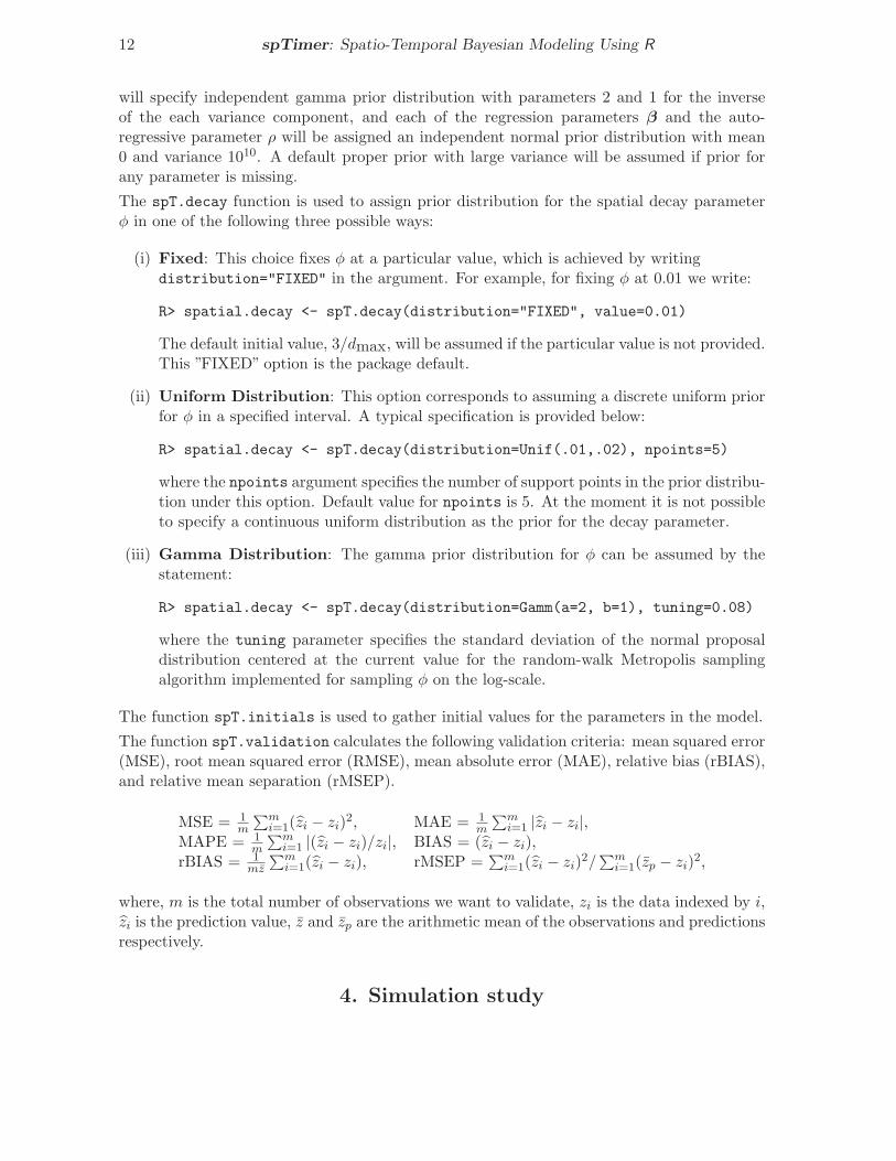
The function spT.validation calculates the following validation criteria: mean squared error(MSE), root mean squared error (RMSE), mean absolute error (MAE), relative bias (rBIAS),and relative mean separation (rMSEP).

MSE = 1m

∑mi=1(zi − zi)

2, MAE = 1m

∑mi=1 |zi − zi|,

MAPE = 1m

∑mi=1 |(zi − zi)/zi|, BIAS = (zi − zi),

rBIAS = 1mz

∑mi=1(zi − zi), rMSEP =

∑mi=1(zi − zi)

2/∑m

i=1(zp − zi)2,

where, m is the total number of observations we want to validate, zi is the data indexed by i,zi is the prediction value, z and zp are the arithmetic mean of the observations and predictionsrespectively.

4. Simulation study

Journal of Statistical Software 13

The main purpose of this example is to validate the body of code underpinning the packagespTimer. The code for carrying out the main inference tasks: estimation of model parametersand predictions are validated for each of three models GP, AR and GPP. This section reportsthe results from experiments on larger data sets using GPP based models. We examinedifferent scenarios, for example an intercept only model and a model with four covariatesto test inference of the regression (β) parameters. We also provide a sensitivity analysis fordifferent signal-to-noise ratios and compare the performance of spTimer with spBayes andmgcv, which adopts a non-Bayesian framework. The code lines for doing this analysis areprovided in the accompanying R file, spTimerdemo.R.

4.1. Simulation design and results

The spatial domain of the simulation study is taken as a square ranging from zero to 1000units, and for fitting GP and AR models we suppose that the sampling locations form aregular grid of 12 × 12 = 144 points (see Figure 1(a)) inside the square. For the GPPbased approximation model we consider 55 × 55 = 3025 grid points inside the square, thatis moderately large (see Figure 1(b)). The number of knots are defined for the GPP basedmodels is a 10×10 square grid inside the range. The temporal domain is taken as 365 days in

0 200 400 600 800 1000

020

040

060

080

010

00

Longitude

Latit

ude

(a)

0 200 400 600 800 1000

020

040

060

080

010

00

Longitude

Latit

ude

(b)

Figure 1: (a) A representation of the 144 grid locations (+) used for simulating the data forGP and AR models. (b) 3025 grid locations (+) are used for data simulation for the GPPbased approximation model and 100 knot points are superimposed using (red) solid circles.

a year. Hence, for GP and AR models we obtain 52, 560(= 144× 365) observations in total,and for the GPP model we generate a data set with 1, 104, 125(= 3025× 365) observations.

Out of these data locations (144 for the GP and AR models; and 3025 for the GPP basedmodel), we randomly choose 10% locations, as validation sites and model data from theremaining 90% sites. Hence, we model data from 129 locations for the GP and AR models

14 spTimer: Spatio-Temporal Bayesian Modeling Using R

and validate them for the set aside data from the remaining 15 locations. Similarly for theGPP based models we set aside data from 300 locations for validations and model data fromthe remaining 2725 locations. We also assume that 5% data are missing at random for theGP, AR and GPP based models. This is done to test the missing data handling capabilities ofthe Bayesian approach which is very common in practice. The Euclidean distance is used inthe simulation study while the real life example in the next section uses the geodetic distancefor a geographic spatial domain. We illustrate throughout using the exponential covariancefunction (ν = 0.5) for both simulation and model fitting, although we have validated usingall other covariance functions.

Three different data sets are simulated from the three models using the following values ofthe model parameters.

We assume that four covariate effects are captured including the intercept term, and take thetrue value of the parameters as β0 = 5.0, β1 = 2.0, β2 = 1.0 and β3 = 0.5. The covariatesx1, . . . , x3 are generated from the standard normal distribution. The spatial effect variance,i.e., the signal σ2

η under GP, AR and GPP based models is assumed to be randomly chosenfrom the uniform distribution in (0, 1) and the pure error (or nugget effect) variance is setat σ2

ǫ = 0.01. We have also provided a sensitivity analysis of the signal-to-noise ratio laterin this section. The spatial decay parameter φ is assumed to be 0.003 that implies highspatial correlation even at large distances. The temporal auto-correlation parameter, ρ is setat 0.2 for the GP and GPP based models. This moderate value was deemed to be enoughfor simulating space-time dependent data over and above the previously assumed high spatialcorrelation. For the AR model, the initial mean and variance for Ol(si, 0) are taken to be 5.0and 0.5 for l = 1. The number of knots for the GPP based model is taken to be 100 (seeFigure 1(b) for their locations) and we assume that the initial values for wl(si, 0) follow thenormal distribution with 0 and variance 0.5 independently for l = 1 under this model.

In this study we illustrate throughout with the Metropolis-Hastings algorithm for simulatingfrom the conditional distribution of the spatial decay parameter since that was found to bethe best among all three methods available in the package (Bakar 2012). In all our MCMCimplementations we use a small number of iterations to choose the tuning parameter (mostlyby trial and error) that achieves an acceptance rate between 15 to 40%, see Section 2.6.For the simulation example, the Gibbs sampler is then run for 5,000 iterations for makinginference with first 1,000 iterations as burn-in. We replicate the experiment 25 times andstore the MCMC iterates of the model parameters, see Table 2 for the summary statistics.

The Gibbs sampler produced estimates of the parameters that were very close to the true sim-ulation values, see Table 2. Moreover, the acceptance rate for sampling the decay parameterφ was also reasonable.

Fitted plots and missing values

Figure 2(a) shows the fitted mean surface plots for time point 5 with the GPP based model.Note that, in this simulation example we only take 30 time points to reduce the computationalburden of model fitting. The fitted surface plot for the mean is obtained using spTimer S3class function plot, by using the argument surface inside the function. The argumentsurface is set to "Mean" or "SD" to plot the fitted mean or standard deviations respectively.It is also possible to change the color pallete of the surface plot using the argument col; forexample, we can use package colorspace and write col=rainbow_hcl(100, start = 200,

Journal of Statistical Software 15

Model Parameter True Value Median 95% Interval

GP

β0 5.0 4.99 (4.96, 5.03)β1 2.0 1.95 (1.83, 2.11)β2 1.0 0.94 (0.80, 1.27)β3 0.5 0.52 (0.46, 0.57)

AR

β0 5.0 5.10 (4.98, 5.27)β1 2.0 1.98 (1.81, 2.30)β2 1.0 1.05 (0.78, 1.21)β3 0.5 0.47 (0.41, 0.55)ρ 0.2 0.19 (0.15, 0.27)

GPP

β0 5.0 4.89 (4.75, 5.13)β1 2.0 1.90 (1.77, 2.07)β2 1.0 0.96 (0.81, 1.13)β3 0.5 0.46 (0.38, 0.55)ρ 0.2 0.17 (0.09, 0.26)

Table 2: True values of the parameters and their estimates using the summary statistics ofthe MCMC samples for all three models. The column Median represents the posterior medianand a 95% credible interval is also provided for each of the parameters.

end = 0). In addition, argument a3d=TRUE can be used to obtain a 3-dimensional plot of thefitted observations. Moreover, contours can be added to the plots. The accompanying R file,spTimerdemo.R contains the detailed code for doing this by sending the fitted model outputto two new functions plot.spT and contour.spT which are also provided. Note that thesefunctions will require the akima (Akima 2013) package.

In Figure 2(b) we provide a residual (z − z) surface plot. We observe that the residualsurface plot varies from -0.4 to 0.4 and in most places the fitted values are close to the trueobservations.

A time series plot of the fitted values is shown in Figure 3(a), for the first location in thesimulated data set, using the GPP model. We see that the fitted mean is very close to thetrue value, and in addition it also shows that the estimates of the missing values are veryclose to the true value. We also provide residual plots for 4 randomly chosen locations inFigure 3(b), where we see the time series plots for the error are close to zero without anyvisible dependence structure. The missing values are indicated by circles, which are fittedusing the Bayesian modeling discussed in Section 2.

Sensitivity of the signal-to-noise ratio (SNR)

We also check the sensitivity of the fit for different signal-to-noise ratio (SNR), i.e., ζ = σ2η/σ

2ǫ ,

through the simulated data. We use 3 different scenarios: (1) σ2η and σ2

ǫ are same, i.e., ζ = 1,(2) when σ2

η is 10 times higher than σ2ǫ , i.e., ζ = 10 and (3) when ζ = 15. We do not allow

ζ to be less than one since it is very unusual for the nugget effect, σ2ǫ , to be larger than the

spatial variance, σ2η.

We simulate data sets in 144 locations for 365 days for the intercept only model defined earlierin Section 4.1. We also replicate the procedure 25 times and obtain the MCMC results for thevariance parameters. Figure 4 shows density plots of ζ for the MCMC samples obtained from

16 spTimer: Spatio-Temporal Bayesian Modeling Using R

0 200 400 600 800 1000

020

040

060

080

010

00

0 2 4 6 8 10

(a) Mean

0 200 400 600 800 1000

020

040

060

080

010

00

−0.4 0.0 0.2 0.4

(b) Residual

Figure 2: Fitted surface plots for (a) mean and corresponding (b) residuals using GPP basedmodel for time point five.

Time series

y

02

46

81

0

1 3 5 7 9 11 14 17 20 23 26 29

True valuesFitted valuesMissing values

(a)

Time series

Err

or

Series 1Series 2Series 3Series 4Missing

−0

.50

.00

.5

1 3 5 7 9 11 14 17 20 23 26 29

(b)

Figure 3: (a) Time-series plots of the true and fitted values at one randomly chosen location.(b) Time-series plots of the residuals at 4 randomly chosen locations.

Journal of Statistical Software 17

the GP model. The true value of ζ is shown using a vertical line. We observe, the distributionof ζ’s for different scenarios include its true value. The MCMC summary statistics for β0, i.e.,the intercept coefficient is given in Table 3. Note that the 95% credible intervals are almosttotally unaffected by the value of ζ.

0 5 10 15 20 25

0.0

0.1

0.2

0.3

0.4

0.5

0.6

0.7

Signal−to−noise ratio (SNR)

N = 15000 Bandwidth = 0.1371

Dens

ity

Distribution of SNR for 1Distribution of SNR for 10Distribution of SNR for 15True SNR values

SNR = 1 SNR = 10 SNR = 15

Figure 4: Distribution of signal-to-noise ratio (SNR), ζ, for 3 different true values: 1, 10 and15.

True β0 Median 95% Interval

ζ = 1 5.0 5.01 (4.96, 5.07)ζ = 10 5.0 4.98 (4.94, 5.03)ζ = 15 5.0 5.02 (4.97, 5.08)

Table 3: Summary statistics for β0 for different scenarios of signal-to-noise ratio (ζ).

4.2. Comparison study

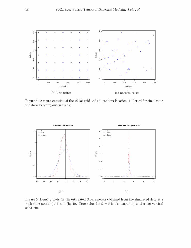
In this section we compare the performance of spTimer models with spBayes and also witha non-Bayesian model, e.g., the additive model as implemented in the mgcv package. Froma modeling perspective we particularly focus on the issues of model fitting, prediction andcomputation time. To proceed, we start with a simple time series data having just 5 timepoints and then increase this to 10, 20 and 60. We simulate 49 locations (see Figure 5(a)) fromthe spatial domain defined in Section 4.1; where in addition to the grid points, the samplinglocations are also chosen randomly, see Figure 5(b). We use the same model parameters asdefined earlier in Section 4.1. Note that in this section we consider the intercept only modeland obtain 4,000 MCMC samples after discarding first 1,000 samples as burn-in.

Figure 6 represents the density plots for the coefficients used in the models. As expected,we observe that all three packages provide estimates of the β0 parameter close to the truevalue. However, we also observe that the estimate obtained from spTimer has a shorter lengthcredible interval than that using the spBayes package.

18 spTimer: Spatio-Temporal Bayesian Modeling Using R

0 200 400 600 800 1000

020

040

060

080

010

00

Longitude

Latit

ude

(a) Grid points

0 200 400 600 800 1000

020

040

060

080

010

00

Longitude

Latit

ude

(b) Random points

Figure 5: A representation of the 49 (a) grid and (b) random locations (+) used for simulatingthe data for comparison study.

4.2 4.4 4.6 4.8 5.0 5.2 5.4 5.6

01

23

4

Data with time point = 5

Den

sity

TrueGAMspBayesspTimer

(a)

0 2 4 6 8 10

01

23

45

6

Data with time point = 10

Den

sity

TrueGAMspBayesspTimer

(b)

Figure 6: Density plots for the estimated β parameters obtained from the simulated data setswith time points (a) 5 and (b) 10. True value for β = 5 is also superimposed using verticalsolid line.

Journal of Statistical Software 19

Table 4 shows a comparison of an approximate computation time for the GP models usingspTimer, and spBayes for data sets with different length of time series. Computation timesfor using the mgcv package are not included in this table since that package does not requirean iterative fitting method such as MCMC. This table clearly shows that spTimer providesfaster model fitting than spBayes when the number of time points in the data is greater thanone. Computation times for implementing the model when there is data for exactly one timepoint are comparable for the spTimer and spBayes packages and hence are not shown here.

Computation timeModels T = 5 T = 10 T = 20 T = 60

GP (spBayes) 3 Minutes 25 Minutes 4 Hours 1 DayGP (spTimer) 10 Seconds 12 Seconds 16 Seconds 40 Seconds

Table 4: Approximate computation time for model fitting using spTimer and spBayes usingdata sets simulated from different time series.

To compare the off-site predictive performance we set aside 20% data for validation purposes.We use a small number of time points T = 5 and a large number T = 60 to comparethe models. We observe that both the validation criteria, MSE and MAE, are smallestfor the spTimer model for the spatio-temporal data, see Table 5. Note that we omit thepredictive results for spBayes at T = 60, because it is computationally prohibitive as itdoes not finish computations for predictions even after running continuously for several days,although the model fitting job finishes within a day as reported in Table 4. We also providefurther comparison of predictive performance of the models using the real life data examplein Section 5.

T = 5 T = 60

Models MSE MAE MSE MAE

Grid basedGP (spTimer) 0.0898 0.2380 0.0759 0.2202GP (spBayes) 1.0692 0.5918 – –GAM (mgcv) 0.1359 0.3021 0.1021 0.2555

RandomGP (spTimer) 0.0970 0.2530 0.0680 0.2090GP (spBayes) 1.0897 0.6306 – –GAM (mgcv) 0.1097 0.2689 0.1004 0.2579

Table 5: Comparison of validation statistics, mean squared error (MSE) and mean absoluteerror (MAE) obtained from spTimer, spBayes and mgcv models.

5. A practical example

We use a real life data set, previously analysed by Sahu and Bakar (2012a), on daily maximum8-hour average ground level ozone concentration for the months of July and August in 2006,observed at 28 monitoring sites in the state of New York. We consider three importantcovariates: maximum temperature (cMAXTEMP in degree Celsius), wind speed (WDSP in nauticalmiles) and percentage average relative humidity (RH) for building a spatio-temporal modelfor ozone concentration. Further details regarding the covariate values and their spatialinterpolation are provided in Bakar (2012). Figure 7 represents a map of the study region

20 spTimer: Spatio-Temporal Bayesian Modeling Using R

Fitted sitesValidation sites

Figure 7: A map of the state of New York showing locations of the 28 ozone monitoring sitesof which data from 8 are used for validation purposes.

together with the 28 monitoring locations of which 8 have been set aside for model validationpurposes. Moreover, we also set aside the data for the last 2 days (August 30 and 31) forvalidating the temporal forecasts. The following set of code lines are used for data preparation.

R> data(NYdata)

R> s<-c(8,11,12,14,18,21,24,28)

R> DataFit<-spT.subset(data=NYdata,

+ var.name=c("s.index"), s=s, reverse=TRUE)

R> DataFit<-subset(DataFit,

+ with(DataFit, !(Day %in% c(30, 31) & Month == 8)))

R> DataValPred<-spT.subset(data=NYdata, var.name=c("s.index"), s=s)

R> DataValPred<-subset(DataValPred,

+ with(DataValPred, !(Day %in% c(30, 31) & Month == 8)))

where, DataFit is for model fitting, and the data sets DataValPred is for model validation.

To fit GP model using spTimer we use the following code:

R> set.seed(11)

R> post.gp <- spT.Gibbs(formula=o8hrmax ~cMAXTMP+WDSP+RH, data=DataFit,

+ model="GP", coords=~Longitude+Latitude, scale.transform="SQRT",

+ spatial.decay=spT.decay(distribution=Gamm(2,1),tuning=0.1))

A number of remarks are in order. The fitted model is the GP model, see Equations 2 and 3.The linear (covariate) part of the model is specified by the formula argument that automat-

Journal of Statistical Software 21

ically includes the intercept. Secondly, the square-root transformation is used, on the fly, tostabilize the variance (Sahu et al. 2007; Sahu and Bakar 2012a). The initial values and thevalues of the hyper-parameters for the prior distributions are assumed by default. Moreover,by default MCMC is run for 5,000 further iterations after discarding first 1,000. The spTimer

user manual lists all the defaults and the ways to change them.

The package spTimer provides the usual R print and summary commands for obtainingsummaries of the model fit. Here is some sample output:

> print(post.gp)

-----------------------------------------------------

Model: GP

Call: o8hrmax ~ cMAXTMP + WDSP + RH

Iterations: 5000

nBurn: 1000

Acceptance rate for phi (%): 32.58

-----------------------------------------------------

Goodness.of.fit Penalty PMCC

values: 253.31 631.76 885.07

-----------------------------------------------------

Computation time: 6.38 - Sec.

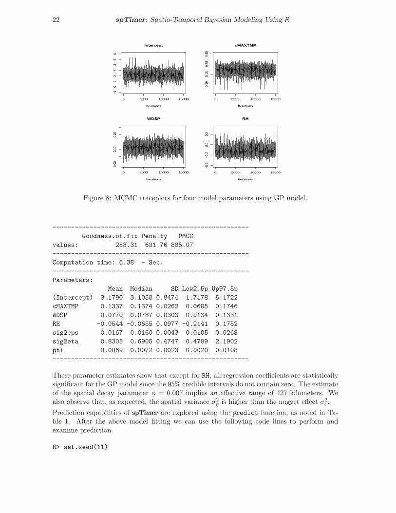
We can also view the MCMC trace plots of the parameters using the plot function as:

R> plot(post.gp)

Figure 8 shows the MCMC trace plots for the four model parameters for 15000 iterations.Further MCMC diagnostics can be done using coda (Plummer, Best, Cowles, and Vines 2012).For example, one can use the code

R> autocorr.diag(as.mcmc(post.gp))

to generate the autocorrelation plots. One can also obtain residual plots using the functionplot with the additional argument residuals=TRUE as:

R> plot(post.gp, residuals=TRUE)

However, none of these plots are included here for brevity.

The predictive model choice criteria (PMCC) described in Section 2.6 is obtained as post.gp$PMCC.We obtain the parameter estimates from the MCMC samples using the familiar summary com-mand:

R> summary(post.gp)

-----------------------------------------------------

Model: GP

Call: o8hrmax ~ cMAXTMP + WDSP + RH

Iterations: 5000

nBurn: 1000

Acceptance rate for phi (%): 32.58

22 spTimer: Spatio-Temporal Bayesian Modeling Using R

0 5000 10000 15000

−10

12

34

56

Intercept

Iterations

0 5000 10000 15000

0.10

0.15

0.20

0.25

cMAXTMP

Iterations

0 5000 10000 15000

0.00

0.10

0.20

WDSP

Iterations

0 5000 10000 15000

−0.4

−0.2

0.0

0.2

RH

Iterations

Figure 8: MCMC traceplots for four model parameters using GP model.

-----------------------------------------------------

Goodness.of.fit Penalty PMCC

values: 253.31 631.76 885.07

-----------------------------------------------------

Computation time: 6.38 - Sec.

-----------------------------------------------------

Parameters:

Mean Median SD Low2.5p Up97.5p

(Intercept) 3.1790 3.1058 0.8474 1.7178 5.1722

cMAXTMP 0.1337 0.1374 0.0262 0.0685 0.1746

WDSP 0.0770 0.0787 0.0303 0.0134 0.1331

RH -0.0544 -0.0655 0.0977 -0.2141 0.1752

sig2eps 0.0167 0.0160 0.0043 0.0105 0.0268

sig2eta 0.8305 0.6905 0.4747 0.4789 2.1902

phi 0.0069 0.0072 0.0023 0.0020 0.0108

-----------------------------------------------------

These parameter estimates show that except for RH, all regression coefficients are statisticallysignificant for the GP model since the 95% credible intervals do not contain zero. The estimateof the spatial decay parameter φ = 0.007 implies an effective range of 427 kilometers. Wealso observe that, as expected, the spatial variance σ2

η is higher than the nugget effect σ2ǫ .

Prediction capabilities of spTimer are explored using the predict function, as noted in Ta-ble 1. After the above model fitting we can use the following code lines to perform andexamine prediction.

R> set.seed(11)

Journal of Statistical Software 23

R> pred.gp <- predict(post.gp, newdata=DataValPred,

+ newcoords=~Longitude+Latitude)

R> print(pred.gp)

--------------------------------------

Spatial prediction with Model: GP

Covariance function: exponential

Distance method: geodetic:km

Computation time: 3.39 - Sec.

--------------------------------------

For model validation spTimer has a built-in function for different validation criteria whichhave been discussed in Section 3.3. Hence, we write:

> spT.validation(DataValPred$o8hrmax,c(pred.gp$Median))

##

Mean Squared Error (MSE)

Root Mean Squared Error (RMSE)

Mean Absolute Error (MAE)

Mean Absolute Percentage Error (MAPE)

Bias (BIAS)

Relative Bias (rBIAS)

Relative Mean Separation (rMSEP)

##

MSE RMSE MAE MAPE BIAS rBIAS rMSEP

43.3210 6.5819 5.0803 11.8626 0.6350 0.0136 0.2621

The spTimer can also perform temporal forecasting at both observed and unobserved locationsusing the same predict function using the additional argument type="temporal", detailsare provided in the package manual.

A predictive map can be drawn using the predictive output obtained from the predict func-tion. Figure 9 for daily ozone concentration levels and their standard deviations on August29, 2006. The accompanying R file spTimerdemo.R provides the code to produce these figures.

We conclude this example with a comparison study with the non-Bayesian generalized additivemodels (Hastie and Tibshirani 1990) using R package mgcv (Wood 2013) as suggested by areferee. The GP models, with typical code as given above, are fitted to the data from the20 fitting sites and then spatial predictions are obtained for the 8 set aside validation sites.The code for implementing this comparison study is provided in the accompanying R file,spTimerdemo.R.

For the additive model we use the gam function and fit additive model and report the predictiveperformance of the model, see Table 6. We observe that the MSE for the Bayesian space-timeGP model is reduced by about 56% compared to the generalized additive models, showingsuperiority of the spatio-temporal models implemented in the package spTimer.

6. Summary

This paper introduces the contributed R package spTimer that enables model fitting, spatialand temporal predictions for large structured point referenced spatio-temporal data sets.

24 spTimer: Spatio-Temporal Bayesian Modeling Using R

Longitude

Latit

ude

20

25

30

35

18

20

20 20

22

24

26

28

30

32

32

34

36

−79 −78 −77 −76 −75 −74 −73 −72

4142

4344

45

18.2

18

4027.9

20.4

36.1

42.825.5

33.9

29.2

29.5

31.6

31.934.1

16.913.4

20.2

17.6

17.5

22.8

27.1

41.6

21

12.4

36.8

17.4

(a)

LongitudeLa

titud

e

6

7

8

9

6

6

6.5

6.5

7

7

7.5

8

8.5

9

9

9.5

−79 −78 −77 −76 −75 −74 −73 −72

4142

4344

45

(b)

Figure 9: Spatially interpolated plots of the daily maximum 8-hour ozone concentration levelsand (b) their standard deviations obtained from the GP models for 29 August, 2006. Actualobservations and their locations are also superimposed in plots (a) and (b) respectively.

Spatial prediction

Models MSE MAE rBIAS rMSEP

Bayesian space-time GP 43.32 5.08 0.01 0.26

non-Bayesian GAM 100.76 7.89 -0.03 0.60

Table 6: Validation statistics for the GP and additive models (GAM).

Journal of Statistical Software 25

Currently, the package is able to analyze data using three substantial and well establishedspatio-temporal models. The package also includes a number of attractive features rangingfrom on the fly transformation to the ability to infer for certain temporal aggregates. Themain body of the code has been validated using a substantial simulation example and a reallife data example.

The underlying code for the package has been written using the C programming language thatis very portable across many different operating systems such as Microsoft Windows, Linuxand Macintosh. The end-user, however, does not need to work with the C language as all theanalysis can be performed by using commands in R. The MCMC based Bayesian hierarchicalmodeling, as implemented in the package, is relatively fast for moderate (a few thousand) tolarge (more than a million) data sets. In particular, the GPP based model is the fastest torun as we have reported in our related work (Sahu and Bakar 2012b).

The package can be extended in several ways, for example, for modeling multivariate dataand for modeling data with a non-Gaussian first stage model. In addition, it will be veryfruitful to add modeling capabilities for spatially varying coefficient process models. Otherpossible extensions include the ability to handle data from sensor networks that vary overtime. Moreover, the implemented models can be enhanced to model mixture of discreteand continuous data such as rainfall. Lastly, extension of the package for handling spatiallymis-aligned data will also be of considerable interest in the literature.

Acknowledgements

The authors thank Dr Philip Kokic, Dr Huidong Jin, Dr Sabyasachi Mukhopadhyay, Mr MarkBass, and two anonymous referees for their many valuable comments on the package and onprevious drafts of this paper.

References

Akima R (2013). akima: Interpolation of Irregularly Space Data. R package version 0.5-11,URL http://cran.r-project.org/web/packages/akima.

Baddeley A, Turner R (2005). “spatstat: An R Package for Analyzing Spatial Point Patterns.”Journal of Statistical Software, 12(6), 1–42.

Bakar KS (2012). Bayesian Analysis of Daily Maximum Ozone Levels. PhD Thesis, Universityof Southampton, Southampton, United Kingdom.

Banerjee S, Carlin BP, Gelfand AE (2004). Hierarchical Modeling and Analysis for SpatialData. Chapman & Hall/CRC, Boca Raton.

Banerjee S, Gelfand AE, Finley AO, Sang H (2008). “Gaussian Predictive Process Models forLarge Spatial Data Sets.” Journal of the Royal Statistical Society B, 70, 825–848.

Bivand RS, Pebesma E, Gomez-Rubio V (2013). Applied Spatial Data Analysis with R, Secondedition. Springer, NY. URL http://www.asdar-book.org/.

26 spTimer: Spatio-Temporal Bayesian Modeling Using R

Cameletti M, Ignaccolo R, Bande S (2009). “Comparing Air Quality Statistical Models.”Technical Report. University of Bergamo, Italy.

Campos G, Rodriguez P (2012). BLR: Bayesian Linear Regression. R package version 1.3,URL http://cran.r-project.org/web/packages/BLR.

Christensen OF, Ribeiro PJ (2002). “geoRglm: A Package for Generalised Linear SpatialModels.” R-NEWS, 2(2), 26–28.

Cressie NAC (1993). Statistics for Spatial Data. John Wiley & Sons, New York.

Cressie NAC, Wikle CK (2011). Statistics for Spatio-Temporal Data. John Wiley & Sons,New York.

Diggle P, Ribeiro PJ (2007). Model-based Geostatistics. Springer, New York.

Finley AO, Banerjee S (2013). spBayes: Univariate and Multivariate Spatial Modeling.R package version 0.3-8, URL http://cran.r-project.org/web/packages/spBayes.

Finley AO, Banerjee S, Carlin BP (2007). “spBayes: An R Package for Univariate andMultivariate Hierarchical Point-referenced Spatial Models.” Journal of Statistical Software,12(4), 1–24.

Finley AO, Sang H, Banerjee S, Gelfand AE (2009). “Improving the Performance of PredictiveProcess Modeling for Large Datasets.” Computational Statistics and Data Analysis, 53,2873–2884.

Furrer R, Nychka D, Sain S (2013). fields: Tools for Spatial Data. R package version 6.9.1,URL http://cran.r-project.org/web/packages/fields.

Gelfand AE (2012). “Hierarchical Modeling for Spatial Data Problems.” Spatial Statistics, 1,30–39.

Gelfand AE, Diggle PJ, Fuentes M, Guttorp P (2010). The Handbook of Spatial Statistics.Chapman & Hall/CRC, New York.

Gelfand AE, Ghosh SK (1998). “Model Choice: A Minimum Posterior Predictive Loss Ap-proach.” Biometrika, 85, 1–11.

Gelfand AE, Smith AFM (1990). “Sampling-Based Approaches to Calculating Marginal Den-sities.” Journal of the American Statistical Association, 85(410), 398–409.

Gelman A, Carlin JB, Stern HS, Rubin DB (2004). Bayesian Data Analysis. 2nd edition.Chapman & Hall/CRC, Boca Raton.

Hadfield JD (2010). “MCMC Methods for Multi-Response Generalized Linear Mixed Models:The MCMCglmm R Package.” Journal of Statistical Software, 33(2), 1–22.

Handcock MS, Stein ML (1993). “A Bayesian Analysis of Kriging.” Technometrics, 35, 403–410.

Handcock MS, Wallis J (1994). “An Approach to Statistical Spatial-Temporal Modelling ofMeteorological Fields.” Journal of the American Statistical Association, 89, 368–390.

Journal of Statistical Software 27

Hastie T (2013). gam: Generalized Additive Models. R package version 1.09, URLhttp://cran.r-project.org/web/packages/gam.

Hastie T, Tibshirani R (1990). Generalized Additive Models. Chapman & Hall, London.

Krige DG (1951). “A Statistical Approach to Some Basic Mine Valuation Problems on theWitwatersrand.”Journal of the Chemical, Metallurgical and Mining Society of South Africa,52, 119–139.

Martin AD, Quinn KM, Park JH (2011). “MCMCpack: Markov Chain Monte Carlo in R.”Journal of Statistical Software, 42(9), 22.

Matern B (1986). Spatial Variation. Second edition. Springer-Verlag, Berlin.

Millo G, Piras G (2012). “splm: Spatial Panel Data Models in R.” Journal of StatisticalSoftware, 47(1), 1–38.

Pebesma E (2012). “spacetime: Spatio-Temporal Data in R.” Journal of Statistical Software,51(7), 1–30.

Pebesma EJ (2004). “Multivariable Geostatistics in S: The gstat Package.” Computers andGeosciences, 30, 683–691.

Pebesma EJ, Bivand RS (2005). “Classes and Methods for Spatial Data in R.” R News, 5(2),9–13.

Pinheiro J, Bates D, DebRoy S, Sarkar D (2013). nlme: Linear andNonlinear Mixed Effects Models. R package version 3.1-113, URLhttp://cran.r-project.org/web/packages/nlme.

Plummer M (2014). rjags: Bayesian Graphical Models using MCMC. R package version 3-12,URL http://cran.r-project.org/web/packages/rjags.

Plummer M, Best N, Cowles K, Vines K (2006). “CODA: Convergence Diagnosis and OutputAnalysis for MCMC.”R News, 6(1), 7–11. URL http://cran.r-project.org/doc/Rnews.

Plummer M, Best N, Cowles K, Vines K (2012). coda: Output Anal-ysis and Diagnostics for MCMC. R package version 0.16-1, URLhttp://cran.r-project.org/web/packages/coda.

R Development Core Team (2006). R: A Language and Environment for Statistical Comput-ing. R Foundation for Statistical Computing, Vienna, Austria. ISBN 3-900051-07-0, URLhttp://www.R-project.org.

Ribeiro PJ, Diggle PJ (2001). “geoR: A Package for Geostatistical Analysis.” R-NEWS, 1(2),14–18. ISSN 1609-3631.

Ripley B (2013). spatial: Functions for Kriging and Point Pattern Analysis. R packageversion 7.3-7, URL http://cran.r-project.org/web/packages/spatial.

Sahu SK, Bakar KS (2012a). “A Comparison of Bayesian Models for Daily Ozone Concentra-tion Levels.” Statistical Methodology, 9(1), 144–157.

28 spTimer: Spatio-Temporal Bayesian Modeling Using R

Sahu SK, Bakar KS (2012b). “Hierarchical Bayesian Autoregressive Models for Large SpaceTime Data with Applications to Ozone Concentration Modelling.” Applied Stochastic Mod-els in Business and Industry, 28, 395–415.

Sahu SK, Gelfand AE, Holland DM (2006). “Spatio-Temporal Modeling of Fine ParticulateMatter.” Journal of Agricultural, Biological, and Environmental Statistics, 11, 61–86.

Sahu SK, Gelfand AE, Holland DM (2007). “High-Resolution Space-Time Ozone Modelingfor Assessing Trends.” Journal of the American Statistical Association, 102, 1221–1234.

Sahu SK, Gelfand AE, Holland DM (2010). “Fusing Point and Areal Level Space-Time Datawith Application to Wet Deposition.” Journal of the Royal Statistical Society C, 59, 77–103.

Spiegelhalter DJ, Thomas A, Best NG (1999). WinBUGS Version 1.2 User Manual. MRCBiostatistics Unit, URL http://www.mrc-bsu.cam.ac.uk/bugs.

Stein ML (1999). Statistical Interpolation of Spatial Data: Some Theory for Kriging. Springer-Verlag, New York.

Sturtz S, Ligges U, Gelman A (2005). “R2WinBUGS: A Package for Running WinBUGSfrom R.” Journal of Statistical Software, 12(3), 1–16.

Venables WN, Ripley BD (2002). Modern Applied Statistics with S. Fourth edition. Springer,New York.

Wood SN (2013). mgcv: Mixed GAM Computation Vehicle with GCV /AIC / REML Smoothness Estimation. R package version 1.7-27, URLhttp://cran.r-project.org/web/packages/mgcv.

Zhang H (2004). “Inconsistent Estimation and Asymptotically Equal Interpolations in Model-based Geostatistics.” Journal of the American Statistical Association, 99, 250–261.

A. Full conditional distributions for the GP model

• The full conditional distribution of β can be obtained from the kernel of (4) as:π(β|..., z) ∼ N(∆χ,∆), where

∆−1 =r∑

l=1

Tl∑

t=1

X′

ltΣ−1η Xlt + Ip/δ

2β

χ =r∑

l=1

Tl∑

t=1

X′

ltΣ−1η Olt.

• Similarly from (4), we sample σ2ǫ and σ2

η from the following conditional distributionsrespectively:

π(1/σ2ǫ |..., z) ∼ G

N

2+ a, b+

1

2

r∑

l=1

Tl∑

t=1

(Zlt −Olt)′(Zlt −Olt)

,

Journal of Statistical Software 29

π(1/σ2η|..., z) ∼ G

N

2+ a, b+

1

2

r∑

l=1

Tl∑

t=1

(Olt −Xltβ)′S−1

η (Olt −Xltβ)

.

• From the kernel of the joint density (4), we obtain the full conditional distributionfor Olt as π(Olt|..., z) ∼ N(∆ltχlt,∆lt), where:

∆−1lt = In/σ

2ǫ +Σ−1

η

χlt = Zlt/σ2ǫ +Σ−1

η Xltβ.

• The full conditional distribution of φ is non-standard and is given by:

π(φ|..., z) ∝ π(φ)×|Sη|−∑

r

l=1Tl/2×exp

− 1

2σ2η

r∑

l=1

Tl∑

t=1

(Olt −Xltβ)′S−1

η (Olt −Xltβ)

.

B. Full conditional distributions for the AR model

• The full conditional distribution of β can be obtained from the joint posteriordistribution of AR models (7) as: π(β|..., z) ∼ N(∆χ,∆), where:

∆−1 =r∑

l=1

Tl∑

t=1

X′

ltΣ−1η Xlt + Ip/δ

2β

χ =r∑

l=1

Tl∑

t=1

X′

ltΣ−1η (Olt − ρOlt).

• The full conditional distribution of ρ can be obtained from (7) as: π(ρ|..., z) ∼N(∆χ,∆), where:

∆−1 =r∑

l=1

Tl∑

t=1

O′

ltΣ−1η Olt + Ip/δ

2ρ

χ =r∑

l=1

Tl∑

t=1

O′

ltΣ−1η (Olt −Xltβ).

• For σ2ǫ and σ2

η we sample from the following conditional distributions respectively:

π(1/σ2ǫ |..., z) ∼ G

N

2+ a, b+

1

2

r∑

l=1

Tl∑

t=1

(Zlt −Olt)′(Zlt −Olt)

,

π(1/σ2η|..., z) ∼ G

N

2+ a, b+

1

2

r∑

l=1

Tl∑

t=1

(Olt − ρOlt−1 −Xltβ)′S−1

η (Olt − ρOlt−1 −Xltβ)

.

• From the joint posterior (7), we obtain the full conditional distribution for Olt

for two cases: (1) when 1 ≤ t ≤ Tl − 1 and (2) when t = Tl. Hence, we writeπ(Olt|..., z) ∼ N(∆ltχlt,∆lt), where:

30 spTimer: Spatio-Temporal Bayesian Modeling Using R

Case 1:

∆−1lt = In/σ

2ǫ + (1 + ρ2)Σ−1

η

χlt = Zlt/σ2ǫ +Σ−1

η (ρOlt−1 +Xltβ + ρ(Olt+1 −Xlt+1β)) .

Case 2:

∆−1lt = In/σ

2ǫ +Σ−1

η

χlt = Zlt/σ2ǫ +Σ−1

η (ρOlt−1 +Xltβ) .

• The full conditional distribution for Ol0 is N(∆lχl,∆l), l = 1, . . . , r where

∆−1l = ρ2Σ−1

η +1

σ2l

S−10

χl = ρ(Ol1 −Xl1β)′Σ−1

η +1

σ2l

µ′

lS−10 .

• We write the full conditional distribution for µl as N(∆lχl,∆l), l = 1, . . . , r, where

∆−1l =

1

σ2l

S−10 +

1

σ2µ

In.

χl =1

σ2l

S−10 Ol0

• The full conditional distribution for σ2l

π(1/σ2l |..., z) ∼ G

(n

2+ a, b+

1

2(Ol0 − µl)

′S−10 (Ol0 − µl)

), l = 1, . . . , r.

• The full conditional distribution of φ parameter is obtained from the kernel (7) as:

π(φ|..., z) ∝ π(φ)× |Sη|−∑

r

l=1Tl/2 ×

exp

− 1

2σ2η

r∑

l=1

Tl∑

t=1

(Olt − ρOlt−1 −Xltβ)′S−1

η (Olt − ρOlt−1 −Xltβ)

×|S0|−r/2 × exp

[−1

2

r∑

l=1

1

σ2l

(Ol0 − µl)′S−1

0 (Ol0 − µl)

].

C. Full conditional distributions for the GPP based AR model

The joint posterior distribution (10) is used to derive the full conditional distributions listedbelow.

• The full conditional distribution of β is N(∆χ,∆) where,

∆−1 =1

σ2ǫ

r∑

l=1

Tl∑

t=1

X ′

ltXlt + Ip/δ2β ,

χ =1

σ2ǫ

r∑

l=1

Tl∑

t=1

X ′

lt(Zlt −Awlt).

Journal of Statistical Software 31

• The full conditional distribution of ρ is N(∆χ,∆)I(0 < ρ < 1) where,

∆−1 =r∑

l=1

Tl∑

t=1

w′

lt−1Σ−1η wlt−1 + Ip/δ

2ρ

χ =r∑

l=1

Tl∑

t=1

w′

lt−1Σ−1η wlt.

• The variance parameters σ2ǫ , σ

2η and σ2

l are sampled from:

π(1/σ2ǫ |..., z) ∼ G

N

2+ a, b+

1

2

r∑

l=1

Tl∑

t=1

(Zlt −Xltβ −Awlt)′(Zlt −Xltβ −Awlt)

π(1/σ2η|..., z) ∼ G

m

∑rl=1 Tl

2+ a, b+

1

2

r∑

l=1

Tl∑

t=1

(wlt − ρwlt−1)′Σ−1

η (wlt − ρwlt−1)

π(1/σ2l |..., z) ∼ G

(m

2+ a, b+

1

2w

′

l0S−10 wl0

), l = 1, . . . , r.

• The full conditional distribution of wlt is given by: N(∆ltχlt,∆lt) where

∆−1lt =

1

σ2ǫ

A′A+ (1 + ρ2)Σ−1η

χlt =1

σ2ǫ

A′(Zlt −Xltβ) + ρΣ−1η (wlt−1 +wlt+1),

for 1 ≤ t ≤ Tl − 1. For t = Tl, we have

∆−1lt =

1

σ2ǫ

A′A+Σ−1η

χlt =1

σ2ǫ

A′(Zlt −Xltβ) + ρΣ−1η wlt−1.

• Full conditional distribution for wl0 is N(∆lχl,∆l), l = 1, . . . , r where

∆−1l = ρ2Σ−1

η +1

σ2l

S−10

χl = ρΣ−1η wl1.

• The full conditional distribution is not available in closed form and it is proportionalto the joint posterior distribution provided in (10), Section 2.4.

Affiliation:

Khandoker Shuvo BakarDepartment of StatisticsYale UniversityNew Haven, CT, 06511, USA.E-mail: Shuvo.Bakar@yale.eduURL: http://statistics.yale.edu/

32 spTimer: Spatio-Temporal Bayesian Modeling Using R

Sujit K. SahuSouthampton Statistical Sciences Research InstituteUniversity of SouthamptonSouthampton, SO17 1BJ, UK.E-mail: S.K.Sahu@soton.ac.ukURL: http://www.soton.ac.uk/~sks/

Journal of Statistical Software http://www.jstatsoft.org/

published by the American Statistical Association http://www.amstat.org/

Volume VV, Issue II Submitted: yyyy-mm-ddMMMMMM YYYY Accepted: yyyy-mm-dd