JOURNAL OF LA Homography Based Egomotion Estimation with …people.inf.ethz.ch/saurero/publications/saurer_2016_homography... · JOURNAL OF LATEX CLASS FILES, VOL. 13, NO. 9, FEBRUARY

JOURNAL OF LATEX CLASS FILES, VOL. 13, NO. 9, FEBRUARY 2016 1

Homography Based Egomotion Estimationwith a Common Direction

Olivier Saurer, Pascal Vasseur, Remi Boutteau, Cedric Demonceaux, Marc Pollefeysand Friedrich Fraundorfer

Abstract—In this paper, we explore the different minimal solutions for egomotion estimation of a camera based on homographyknowing the gravity vector between calibrated images. These solutions depend on the prior knowledge about the reference plane usedby the homography. We then demonstrate that the number of matched points can vary from two to three and that a direct closed-formsolution or a Grobner basis based solution can be derived according to this plane. Many experimental results on synthetic and realsequences in indoor and outdoor environments show the efficiency and the robustness of our approach compared to standardmethods.

Index Terms—Computer vision, egomotion estimation, homography estimation, structure-from-motion.

F

1 INTRODUCTION

NOWADAYS, point-based methods to estimate themotion of a camera are well known. If the camera is

uncalibrated, eight or seven points are needed to estimatethe fundamental matrix between two consecutive views [1].When the intrinsic parameters of the camera are known,five points are then enough to estimate the essential matrix[2]. To decrease the sensitivity of these methods, a robustframework such as Random Sample Consensus (RANSAC)is necessary. Thus, reducing the number of needed matchedpoints between views is important in terms of computationefficiency and of robustness improvement. For example, asshown in Figure 1, for a probability of success of 0.99 and arate of outliers equal to 0.5, the number of RANSAC trialsis divided by eight, if five points are used instead of eight.In the case of a robust estimation based on eight points,1177 trials are necessary whereas 145 are sufficient if onlyfive points are required. Thus, finding a minimal solutionfor egomotion estimation is important for robust real timeapplications.

However, reducing the number of necessary pointsis only possible if some hypotheses or supplementarydata are available. For example, if we know a commondirection between the two views, three points can thenbe used to estimate the full essential matrix [3]. Extreme

• Olivier Saurer and Marc Pollefeys are with the Computer Vision andGeometry Group in the Department of Computer Science, ETH Zurich,Switzerland.E-mail: [email protected], [email protected]

• Pascal Vasseur is with LITIS, Universite de Rouen, France.E-mail: [email protected]

• Remi Boutteau is with IRSEEM, ESIGELEC, Rouen, France.E-mail: [email protected]

• Cedric Demonceaux is with Le2i, UMR CNRS 6306 Universite deBourgogne, France.E-mail: [email protected]

• Friedrich Fraundorfer is with the Institute for Computer Graphics andVision, TU Graz, Austria.E-mail: [email protected]

Manuscript received February 16, 2016; revised ?? ??, 20??.

situations appear when a planar non-holonomic motion issupposed [4] or when the metric velocity of a single cameracan be estimated knowing its attitude and its acceleration[5]. In these cases, only one point allows to estimate themotion. These initial hypotheses or additional knowledgescan then deal with the pose of the camera or with the 3Dstructure of the scene. For example, if the 3D points belongto a single plane, the egomotion estimation is reduced toa homography computation between two views, that canbe calculated using only four points [1]. In many scenesand many applications, the scene plane hypothesis seemssuitable. Indeed, in many scenarios such as indoor or streetcorridors and more generally in man made environments,this assumption holds.

Thus, in this paper we investigate the cases whereat least one plane is present in the scene and wherewe have some partial knowledge about the pose of thecamera. We suppose that we are able to extract a commondirection between consecutive views and we can have someinformation about the normal of the considered plane.Obtaining a common direction can be easily performedthanks to an IMU (Inertial Measurement Unit) associatedwith the camera, which is often the case in mobile devicesor UAV (Unmanned Aerial Vehicle). The coupling with acamera is then very easy and can then be used for differentcomputer vision tasks [6], [7], [8], [9], [10]. Without anyexternal sensor, this common direction can also be directlyextracted from the images thanks to vanishing points [11]or horizon detection [12].

In this work, assuming the roll and pitch angles of thecamera as known, we propose to find a minimal closed-form solution for homography estimation in man madeenvironments. We will derive different solutions dependingon the prior knowledge about the 3D scene :

• If the extracted points lie on the ground plane, wewill see that only two points are required to estimate


0 0.1 0.2 0.3 0.4 0.5 0.6 0.7 0.8 0.9100

101

102

103

104

105

106

107

108

Ratio of outliers

Num

ber o

f iter

ation

s

Three pointsFour pointsFive pointsEight pointsTwo points

Fig. 1. Comparison of the RANSAC iteration number for 99% of successprobability

the camera egomotion. In this case, the solution isunique and contrary to the other algorithms for es-sential matrix estimation, there is no supplementaryverification for finding the good solutions among thedifferent possibilities.

• If the considered points are on a vertical plane, wepropose an efficient 2.5pt formulation in order toretrieve the motion of the camera and the normal ofthe plane related to the pose of the camera. This so-lution allows for an early reject of a pose hypothesisby including a consistency check on the three pointcorrespondences.

• If the plane orientation is completely unknown, wedevelop a minimal solution using only three pointsinstead of four points needed in the classical homog-raphy estimation.

All these methods will be evaluated on synthetic and realdata and compared with different methods proposed in theliterature.The rest of the paper is organized as follows. In the secondpart, we describe the different existing methods in theliterature which deal with minimal solution for egomotionestimation. In the next section, we explain how to reduce thenumber of points for estimating the homography betweentwo views and derive the proposed solutions accordingto the prior knowledge. In the fourth section, we showthe behaviour of our solutions on synthetic and real dataand compare with other classical methods in a quantitativeevaluation. Finally, we will conclude by providing someextents to this work.

2 RELATED WORKS

When the camera is not calibrated, at least 8 or 7 pointsare needed to recover the motion between views [1]. It’swell known, that if the camera is calibrated, only 5 featurepoint correspondences are sufficient to estimate the relativecamera pose. Reducing this number of points can be veryinteresting in order to reduce the computation time and toincrease the robustness when using a robust estimator suchas RANSAC. The reduction of the degree of freedom (DoF)number and consequently the number of matched pointsbetween images can be achieved by introducing someconstraints on the camera motion (planar for example) orthe feature points (on the same plane) or by using someadditional information provided by other sensors such as

IMU for instance.

For example, if all the 3D points lie on a plane, aminimum of 4 points is required to estimate the motion ofthe camera between two-views [1]. On the other hand, ifthe camera is embedded on a mobile robot which moveson a planar surface, only 2 points are required to recoverthe motion [13] and if in addition the mobile robot hasnon-holonomic constraints only one point is necessary [4].Similarly, if the camera moves in a plane perpendicular tothe gravity, 1 point correspondence is sufficient to recoverthe motion as shown by Troiani et al. [14].

The number of points needed to estimate the egomotioncan be also reduced if some information about the relativerotation between two poses are available. This informationcan be given by vanishing points extraction in the images[15] or by taking into account extra information given byan additional sensor. Thus, Li et al. [16] show that in thecase of an IMU associated to the camera, only 4 points aresufficient to estimate the relative motion even if the extrinsiccalibration between the IMU and the camera is not known.

Similarly, some different algorithms have been recentlyproposed in order to estimate the relative pose betweentwo cameras by knowing a common direction. It has beendemonstrated that knowing roll and pitch angles of thecamera at each frame, only three points are needed torecover the yaw angle and the translation of the cameramotion up to scale [3], [17], [18]. In these approaches, onlythe formulation of the problem is different and consequentlythe way to solve it. All these works start with a simplifiedessential matrix in order to derive a polynomial equationsystem. For example, in [17], their parametrization leadsto 12 solutions by using the Macaulay matrix method. Thecorrect solution has then to be found among a set of possiblesolutions. The approach presented in [3] permits to obtaina 4th-order polynomial equation and consequently leadsto a more efficient solution. In [18], the authors propose aclosed-form solution to this 4th-order polynomial equationthat allows a faster computation.

For a further reduction of necessary feature points,stronger hypotheses have to be added. If the completerotation between the two views are known, only 2 degreesof freedom corresponding to the translation up-to-scale hasto be estimated and consequently 2 points are sufficientto solve the problem [19], [20]. In this case, the authorscompute the translation vector using the epipolar geometrygiven the rotation. Thus, these approaches allow to reducethe number of points but also imply the knowledge ofthe complete rotation between two views making the poseestimation very sensitive to IMU inaccuracy. More recently,Martinelli [21] proposes a closed-form solution for structurefrom motion knowing the gravity axis of the camera in amultiple view scheme. He shows that at least three featurepoints lying on a same plane and three consecutive viewsare required to estimate the motion. In the same way, theplane constraint has been used for reducing the complexityof the bundle adjustment (BA) in a visual simultaneouslocalization and mapping (SLAM) embedded on a micro-aerial vehicle (MAV) [22].

Most closely related papers to our approach are theworks of [3], [18] in which they simplify the essential matrix


knowing the vertical of the cameras. In this work, to reducethe number of points, rather than deriving the epipolarconstraint to compute the essential matrix, we propose touse the homography constraint between two views. Thus,we suppose that a significant plane exists in the sceneand that the gravity direction is known. Let us note thatrecently, in [23] Troiani et al. have also proposed a methodusing 2 points on the ground plane with the knowledge ofthe vertical of the camera. However, they do not use thehomography formalism and their method requires to knowthe distance between the two 3D points. In our method,this hypothesis is not necessary and we only assume thatthe points lie on a same plane. The Manhattan worldassumption [24] has also recently successfully been usedfor multi-view stereo [25], the reconstruction of buildinginteriors [26] and also for scene reconstruction from a singleimage only [27]. Our contribution differs from them, as wecombine gravity measurements with the weak Manhattanworld assumption. This paper is an extension of [28], [29]where we studied camera pose estimation based on homo-graphies with a common vertical direction and a known orat least partially known plane normal. In [28] we proposeda homography based pose estimation algorithm that doesnot require any knowledge on the plane normal. In factthe algorithm provides the plane normal in addition to thecamera pose.

3 MOTION ESTIMATION

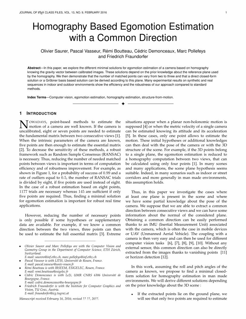
Knowing the vertical direction in images will simplify theestimation of camera pose and camera motion, which arefundamental methods in 3D computer vision. It is thenpossible to align every camera coordinate system with themeasured vertical direction such that the z-axis of the cam-era is parallel to the vertical direction and the x-y-plane ofthe camera is orthogonal to the vertical direction (illustratedin Fig. 2). In addition, this would mean that the x-y-plane ofthe camera is now parallel to the world’s ground plane andthe z-axis is parallel to vertical walls.

General case Aligned with gravity direction

gra

vit

y

Fig. 2. Alignment of the camera with the gravity direction.

This alignment can just be done as a coordinate trans-form for motion estimation algorithms, but also be im-plemented as image warping such that feature extractionmethods benefit from it. Relative motion between two suchaligned cameras reduces to a 3-DOF motion, which consistsof 1 remaining rotation and a 2-DOF translation vector (i.e.,a 3D translation vector up to scale).

The algorithms for estimating the relative pose are de-rived from a homography formulation, where a plane is ob-served in two images. The homography is then decomposedinto a relative rotation and translation between the twoimages. By incorporating the known vertical direction, the

parametrization of the pose estimation problem is greatlyreduced from 5-DOF to 3-DOF. This simplification leads toa closed-form 2pt and a 2.5pt algorithm to compute thehomography. By relaxing the assumption of strictly verticalor horizontal structures and making use of the knowngravity direction, the homography formulation results in aclosed form solution requiring 3-points only.

In the following subsections we derive the 2pt algorithmfor the known plane normal cases (ground and verticalplane), then we provide a derivation of the 2.5pt and 3ptalgorithm for a known gravity direction with an unknownplane orientation.

3.1 2pt Relative Pose for Points on the Ground Plane

The general homographic relation for points belonging to a3D plane and projected in two different views is defined asfollows :

qj = Hqi, (1)

with qi = [xi, yi, wi]> and qj = [xj , yj , wj ]

> the projectivecoordinates of the points between the views i and j. H isgiven by:

H = R− 1

dtn>, (2)

where R and t are respectively the rotation and the trans-lation between views i and j and where d is the distancebetween the camera i and the 3D plane described by thenormal n.In our case, we assume that the camera intrinsic parametersare known and that the points qi and qj are normalized.We also consider that the attitude of the cameras for theboth views are known and that these attitude measurementshave been used to align the camera coordinate system withthe ground plane. In this way, only the yaw angle θ betweenthe two views remains unknown. Therefore equation 2 canbe expressed as:

H = Rz −1

dtn, (3)

where Rz denotes the unknown rotation around the yawangle (z-axis). Similarly, since we consider that the groundplane constitutes the visible 3D plane during the movementof the camera, we can note that n = [0, 0, 1]>.Consequently, equation 3 can be written as:

H =

cos(θ) − sin(θ) 0sin(θ) cos(θ) 0

0 0 1

− td

001

> , (4)

d being unknown, the translation can be known only up toscale. Consequently, the camera-plane distance d is set to 1and absorbed by t. We then obtain:

H =


0 0 1

− txtytz

001

> , (5)

=

cos(θ) − sin(θ) −txsin(θ) cos(θ) −ty

0 0 1− tz

. (6)


In a general manner, this homography can beparametrized as

H =

h1 −h2 h3

h2 h1 h4

0 0 h5

. (7)

The problem consists of solving for the five entries of thehomography H. We consider the following relation:

qj ×Hqi = 0, (8)

where × denotes the cross product. By rewriting the equa-tion, we obtain:

xjyjwj

× h1 −h2 h3

h2 h1 h4

0 0 h5

xiyiwi

= 0. (9)

This gives us three equations, where two of them arelinearly independent. We expand the above equation andconsider only the first two linearly independent equations,which results in:

[−wjyih1 − wjxih2 − wiwjh4 + wiyjh5

wjxih1 − wjyih2 + wiwjh3 − wixjh5

]= 0. (10)

The equation system can be re-written into:

[−wjyi −wjxi 0 −wiwj wiyjwjxi −wjyi wiwj 0 −wixj

]h1

h2

h3

h4

h5

= 0.

(11)The above equation represents a system of equations of

the form Ah = 0. It is important to note that A has rank4. Since each point correspondence gives rise to two inde-pendent equations, we require two point correspondencesto solve for h up to one unknown scale factor. The singularvector of A, which has the smallest singular value spansa one dimensional (up to scale) solution space. We chosethe solution h such that ||h|| = 1. Then, to obtain validrotation parameters we enforce the trigonometric constrainth2

1 + h22 = 1 on h, by dividing the solution vector by

±√h2

1 + h22. The camera motion parameters, can directly be

derived from the homography:

t =[−h3, −h4, 1− h5

]>, (12)

R =

h1 −h2 0h2 h1 00 0 1

. (13)

Due to the sign ambiguity in ±√h2

1 + h22 we obtain two

possible solutions for R and t. An alternative solution isproposed in Appendix A which uses an inhomogeneoussystem of equations to solve for the unknown camera pose.

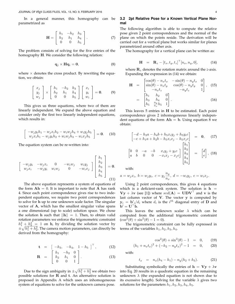
3.2 2pt Relative Pose for a Known Vertical Plane Nor-malThe following algorithm is able to compute the relativepose given 2 point correspondences and the normal of theplane on which the points reside. The derivation will becarried out for a vertical plane but works similar for planesparametrized around other axis.

The homography for a vertical plane can be written as:

H = Rz − [tx, ty, tz]>[nx, ny, 0], (14)

where Rz denotes the rotation matrix around the z-axis.Expanding the expression in (14) we obtain:

H =

cos(θ)− nxtx − sin(θ)− nytx 0sin(θ)− nxty cos(θ)− nyty 0−nxtz −nytz 1

, (15)

=

h1 h2 0h3 h4 0h5

ny

nxh5 1

. (16)

This leaves 5 entries in H to be estimated. Each pointcorrespondence gives 2 inhomogeneous linearly indepen-dent equations of the form Ah = b. Using equation 8 weobtain:

[−d− h3a− h4b+ h5xiyj + h5yic−e+ h1a+ h2b− h5xixj − h5xjc

]= 0, (17)

[0 0 −a −b xiyj + yica b 0 0 −xixj − xjc

]h1

h2

h3

h4

h5

=

[de

], (18)

with:

a = wjxi, b = wjyi, c = yjnynx, d = −wiyj , e = wixj .

Using 2 point correspondences, this gives 4 equationswhich is a deficient-rank system. The solution is h =Vy + λv (see [1]) where svd(A) = UDV> and v is thelast column vector of V. The vector y is computed byyi = b′i/di where di is the ith diagonal entry of D andb′ = U>b.

This leaves the unknown scalar λ which can becomputed from the additional trigonometric constraint(cos2(θ) + sin2(θ)− 1 = 0).

The trigonometric constraint can be fully expressed interms of the variables h1, h2, h3, h4.

cos2(θ) + sin2(θ)− 1 = 0, (19)(h1 + nxtx)2 + (−h2 − nytx)2 − 1 = 0, (20)

with:

tx = nx(h4 − h1)− ny(h2 + h3). (21)

Substituting symbolically the entries of h = Vy + λvinto Eq. 20 results in a quadratic equation in the remainingunknown λ (the expanded equation is not shown due toits excessive length). Solving for the variable λ gives twosolutions for the parameters h1, h2, h3, h4, h5.


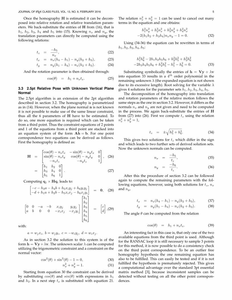
Once the homography H is estimated it can be decom-posed into relative rotation and relative translation param-eters. We back-substitute the entries of H from (16), that ish1, h2, h3, h4 and h5 into (15). Knowing nx and ny , thetranslation parameters can directly be computed using thefollowing relations:

tz =−h5

nx, (22)

tx = nx(h4 − h1)− ny(h2 + h3), (23)ty = ny(h1 − h4)− nx(h2 + h3). (24)

And the rotation parameter is then obtained through:

cos(θ) = h1 + nxtx. (25)

3.3 2.5pt Relative Pose with Unknown Vertical PlaneNormalThe 2.5pt algorithm is an extension of the 2pt algorithmdescribed in section 3.2. The homography is parametrizedas in (14). However, when the plane normal n is not knownit is not possible to make use of the same linear constraint,thus all the 6 parameters of H have to be estimated. Todo so, one more equation is required which can be takenfrom a third point. Thus the constraint equations of 2 pointsand 1 of the equations from a third point are stacked intoan equation system of the form Ah = b. For one pointcorrespondence two equations can be derived as follows.First the homography is defined as:

H =

cos(θ)− nxtx − sin(θ)− nytx 0sin(θ)− nxty cos(θ)− nyty 0−nxtz −nytz 1

, (26)

=

h1 h2 0h3 h4 0h5 h6 1

. (27)

Computing qj ×Hqi leads to:[−c− h3a− h4b+ h5xiyj + h6yiyj−d+ h1a+ h2b− h5xixj − h6xjyi

]= 0, (28)

[0 0 −a −b xiyj yiyja b 0 0 −xixj −xjyi

]h1

h2

h3

h4

h5

h6

=

[cd

],(29)

with:

a = wjxi, b = wjyi, c = −wiyj , d = wixj .

As in section 3.2 the solution to this system is of theform h = Vy+λv. The unknown scalar λ can be computedutilizing the trigonometric constraint and a constraint on thenormal vector:

cos2(θ) + sin2(θ)− 1 = 0, (30)n2x + n2

y = 1. (31)

Starting from equation 30 the constraint can be derivedby substituting cos(θ) and sin(θ) with expressions in h1

and h2. In a next step tx is substituted with equation 21.

The relation n2x + n2

y = 1 can be used to cancel out manyterms in the equation and one obtains:

h21n

2y + h2

2n2x + h2

3n2y + h2

4n2x

−2(h1h2 + h3h4)nxny − 1 = 0. (32)

Using (34-36) the equation can be rewritten in terms ofh1, h2, h3, h4, h5:

h21h

26 − 2h1h2h5h6 + h2

2h25 + h2

3h26

−2h3h4h5h6 + h24h

25 − h2

5 − h26 = 0. (33)

Substituting symbolically the entries of h = Vy + λvinto equation 33 results in a 4th order polynomial in theremaining unknown λ (the expanded equation is not showndue to its excessive length). Root solving for the variable λgives 4 solutions for the parameter sets h1, h2, h3, h4, h5.

The decomposition of the homography into translationand rotation parameters of the relative motion follows thesame steps as the one in section 3.2. However, it differs as thenormals nx and ny are not given and need to be computedin the process. We again back-substitute the entries of Hfrom (27) into (26). First we compute tz using the relationn2x + n2

y = 1,

tz = ±√h2

5 + h26. (34)

This gives two solutions for tz which differ in the signand which leads to two further sets of derived solution sets.Now the unknown normals can be computed.

nx =−h5

tz, (35)

ny =−h6

tz. (36)

After this the procedure of section 3.2 can be followedagain to compute the remaining parameters with the fol-lowing equations, however, using both solutions for tz , nxand ny ,

tx = nx(h4 − h1)− ny(h2 + h3), (37)ty = ny(h1 − h4)− nx(h2 + h3). (38)

The angle θ can be computed from the relation

cos(θ) = h1 + nxtx. (39)

An interesting fact in this case is, that only one of the twoavailable equations from the third point is used. Althoughfor the RANSAC loop it is still necessary to sample 3 pointsfor this method, it is now possible to do a consistency checkon the third point correspondence. To be an outlier freehomography hypothesis the one remaining equation hasalso to be fulfilled. This can easily be tested and if it is notfulfilled the hypothesis is prematurely rejected. This givesa computational advantage over the standard 3pt essentialmatrix method [3], because inconsistent samples can bedetected without testing on all the other point correspon-dences.


3.4 3pt Relative Pose using the Homography Con-straintIn this section we discuss a 3pt formulation of the camerapose estimation with a known vertical direction. It differsfrom the algorithms in the previous section as it does notneed the presence of scene planes. A 3pt algorithm hasalready been presented by [3] but using an essential matrixformulation. With this 3pt algorithm we propose an alter-native to the previous essential matrix algorithm but basedon a homography formulation. We start from (14), insteadof assuming the plane to be parallel to the gravity vectorwe don’t make any assumption on the plane orientation andtherefore use 3 parameters nx, ny, nz , for the fully unknownplane normal, which leads to:

H = Rz − [tx, ty, tz]>[nx, ny, nz]. (40)

The camera-plane distance is absorbed by t the same wayas in the previous sections.

The homography matrix then consists of the followingentries:

H =

cos(θ)− txnx − sin(θ)− txny −txnzsin(θ)− tynx cos(θ)− tyny −tynz−tznx −tzny 1− tznz

. (41)

The unknowns we are seeking for are the motion pa-rameters cos(θ), sin(θ), tx, ty, tz and the normal [nx, ny, nz]of the plane spanned by the 3 point correspondences. Re-call that the standard 3pt essential matrix algorithm onlysolves for the camera motion, while the 3pt homographyalgorithm provides the camera motion and a plane normalwith the same number of correspondences. To solve forthe unknowns we setup an equation system of the form:qj × Hqi = 0 and expand the relations to obtain thefollowing two polynomial equations:

aty − btz − wjxi sin(θ)− wjyi cos(θ) + yjwi = 0, (42)−atx + ctz + wjxi cos(θ)− wjyi sin(θ)− xjwi = 0, (43)

where:

a = wjxinx + wjyiny + wjnzwi,

b = yjwinz + yjnxxi + yjnyyi, (44)c = xjnxxi + xjwinz + xjnyyi.

The third equation obtained from qj ×Hqi = 0 is omittedsince it is a linear combination of the two other equations.Therefore each point correspondence gives 2 linearly inde-pendent equations and there are two additional quadraticconstraints, the trigonometric constraint and the unit lengthof the normal vector that can be utilized:

sin2(θ) + cos2(θ) = 1, (45)n2x + n2

y + n2z = 1. (46)

The total number of unknowns is 8 and the two quadraticconstraints together with the equations from 3 point cor-respondences give a total of 8 polynomial equations inthe unknowns. An established way to find an algebraicsolution to such a polynomial equation system is by usingthe Grobner basis technique [30]. By computing the Grobner

TABLE 1Comparison of the degenerate conditions (yes means degenerate) forthe standard 3pt method, the proposed 3pt homography method, the

2pt methods and the 2.5pt method.

3pt-essential 3pt-hom 2pt 2.5ptcollinear points no yes no nocollinear points parallelto translation direction

yes yes no no

points coplanar totranslation vector

yes yes no no

basis a univariate polynomial can be found which allowsto find the value of the unknown variable by root solving.The remaining variables can then be computed by back-substitution. To solve our problem we use the automaticGrobner basis solver by Kukelova et al. [31], which can bedownloaded at the authors webpage. The software automat-ically generates Matlab-Code that computes a solution to thegiven polynomial equation system (in our case the abovespecified 8 equations). The produced Matlab-Code consistsof 299 lines and thus cannot be given here. The analysis ofthe Grobner basis solutions shows, that the final univariatepolynomial has degree 8, which means that there are up to8 real solutions to our problem.

3.5 Degenerate Configurations

In this section we discuss the degenerate conditions forthe proposed algorithms. In previous works [3], [18], [17]the degenerate conditions for the standard 3pt methodfor essential matrix estimation have been investigated indetail. In these papers multiple degenerate conditions areidentified. It is also pointed out that a collinear configura-tion of 3D points is in general not a degenerate conditionfor the 3pt method, while it is one for the 5pt method.Degenerate conditions for the standard 3pt algorithm how-ever are collinear points that are parallel to the translationdirection and points that are coplanar to the translationvector. We investigated if these scenarios also pose degen-erate conditions for our proposed algorithms, the 2pt, 2.5ptand 3pt homography method by conducting experimentswith synthetic data. Degenerate cases could be identifiedby a rank loss of the equation system matrix or for theGrobner basis case as a rank loss of the action matrix. Forthe 3pt homography case this revealed that the proposedmethod shares the degenerate conditions of the standard 3ptmethod but in addition also has a degenerate condition forthe case of collinear points. This is understandable as the3pt homography method also solves for the plane normalwhich then has an undefined degree of freedom around theaxis of the collinear points. For the 2pt (both 2pt methodsshare the same properties) and 2.5pt algorithm these specialcases however, do not pose degenerate conditions. Moreinformation in case of knowledge or partial knowledge ofplane parameters allows to avoid degeneracy in the casescritical for the more general 3pt methods. The results of thecomparison are summarized in Table 1.


4 EXPERIMENTS

4.1 Synthetic EvaluationTo evaluate the algorithms on synthetic data we chose thefollowing setup. The average distance of the scene to thefirst camera center is set to 1. The scene consists of twoplanes, one ground plane and one vertical plane whichis parallel to the image plane of the first camera. Bothplanes consist of 200 randomly sampled points. The base-line between two cameras is set to be 0.2, i.e., 20% of theaverage scene distance, and the focal length is set to 1000pixels, with a field of view of 45 degrees.Each algorithm is evaluated under varying image noise andincreasing IMU noise. Each of the two setups is evaluatedunder a forward, into the scene (along the z-axis) and asideways (along the x-axis) translation of the second camera.In addition the second camera is rotated around each axis.

To evaluate the robustness of the algorithms we comparethe relative translation and rotation separately. The errormeasure compares the angle difference between the truerotation and the estimated rotation. Since the translation isonly known up to scale, we compare the angle between thetrue- and estimated translation. The errors are computed asfollows:

• Angle difference in R:ξR = arccos((Tr(RR>)− 1)/2)

• Direction difference in t:ξt = arccos((t>t)/(‖t‖‖t‖))

Where R, t denote the ground-truth transformation and R,t are the corresponding estimated transformations.

Each data point in the plots represents the 5-quantile1

(Quintiles) of 1000 measurements.

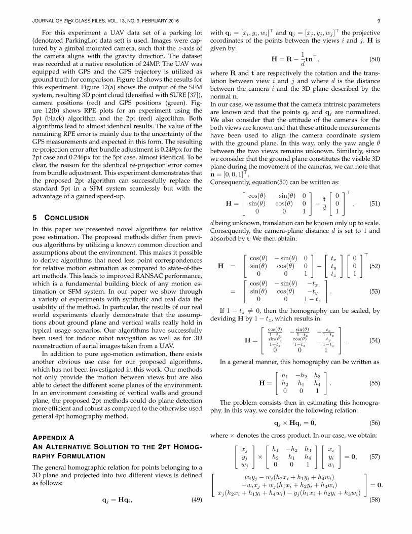
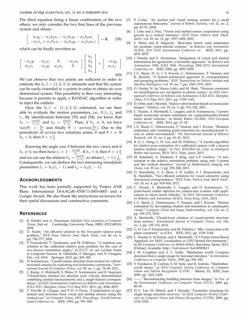
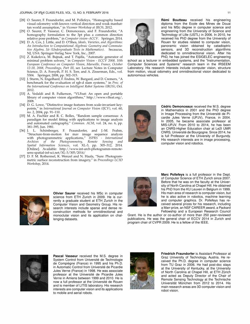
4.1.1 Relative PoseFig. 3 and Fig. 4 compare the 2-point algorithm to the gen-eral 5pt-essential matrix [2], 4pt-homography [1] and 3pt-essential matrix [3] algorithms. Notice, in these experimentsthe camera poses were computed from points randomlydrawn from the ground plane. Since camera poses estimatedfrom coplanar points do not provide a unique solution forthe 5pt, 4pt and 3pt-essential matrix algorithm we evaluateeach hypothesis with all points coming from both planes.The solution providing the most inliers is chosen to be thecorrect one. This evaluation is used in all our syntheticexperiments. Similarly Fig. 5 and Fig. 6 show a comparisonof the 2.5pt algorithm with the general 5pt, the 4pt and the3pt-essential matrix algorithms. Here the camera poses arecomputed from points randomly sampled from the verticalplane only.The evaluation shows that knowing the vertical directionand exploiting the planarity of the scene improves motionestimation. The 2pt and 2.5pt algorithms outperform the5pt and 4pt algorithm, in terms of accuracy. Under perfectIMU measurements the algorithms are robust to imagenoise and perform significantly better than the 5pt and 4ptalgorithm. With increasing IMU noise their performance arestill comparable to the 5pt algorithm and superior to the 4ptalgorithm.

1. The k-quantile represents the boundary value of the kth intervalwhen dividing ordered data into k regular intervals. For k = 2, the2-quantile represents the median value.

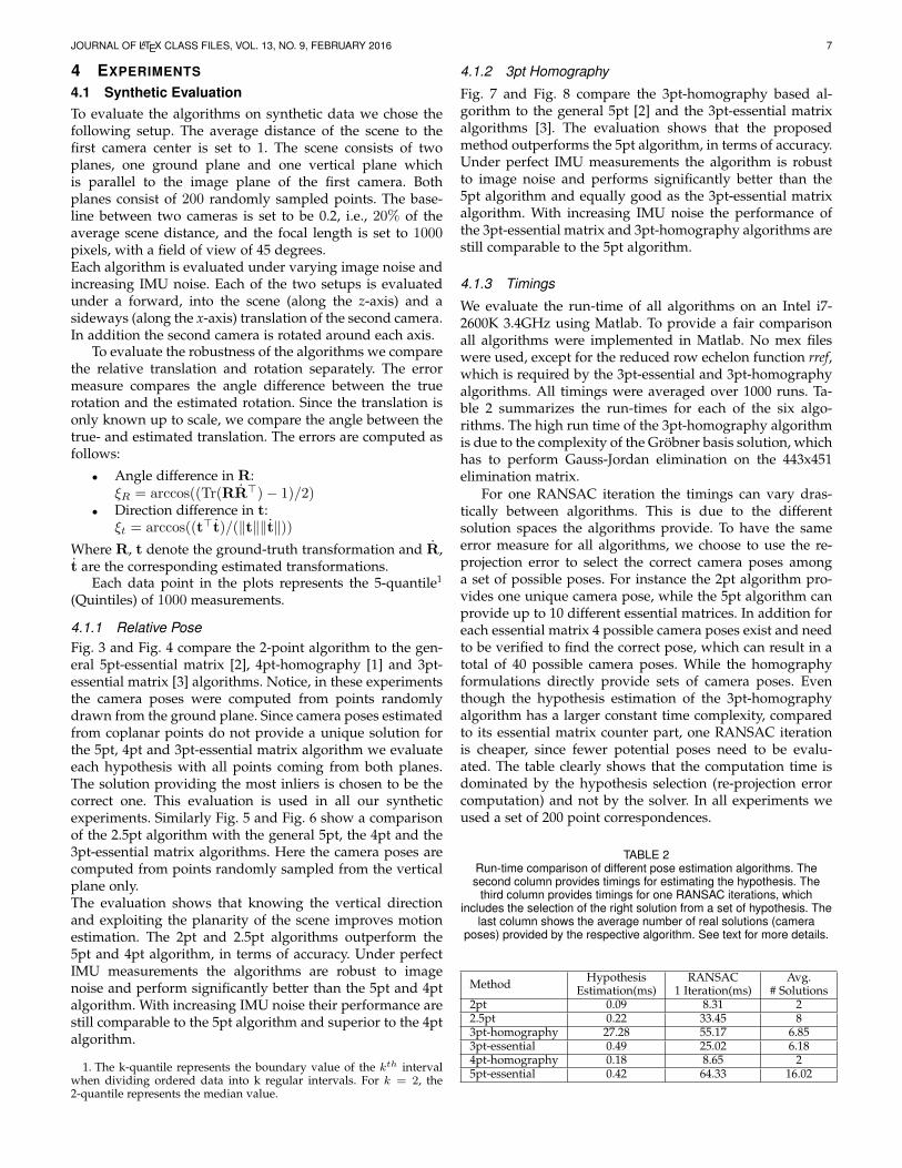
4.1.2 3pt Homography

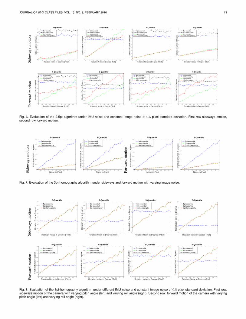
Fig. 7 and Fig. 8 compare the 3pt-homography based al-gorithm to the general 5pt [2] and the 3pt-essential matrixalgorithms [3]. The evaluation shows that the proposedmethod outperforms the 5pt algorithm, in terms of accuracy.Under perfect IMU measurements the algorithm is robustto image noise and performs significantly better than the5pt algorithm and equally good as the 3pt-essential matrixalgorithm. With increasing IMU noise the performance ofthe 3pt-essential matrix and 3pt-homography algorithms arestill comparable to the 5pt algorithm.

4.1.3 Timings

We evaluate the run-time of all algorithms on an Intel i7-2600K 3.4GHz using Matlab. To provide a fair comparisonall algorithms were implemented in Matlab. No mex fileswere used, except for the reduced row echelon function rref,which is required by the 3pt-essential and 3pt-homographyalgorithms. All timings were averaged over 1000 runs. Ta-ble 2 summarizes the run-times for each of the six algo-rithms. The high run time of the 3pt-homography algorithmis due to the complexity of the Grobner basis solution, whichhas to perform Gauss-Jordan elimination on the 443x451elimination matrix.

For one RANSAC iteration the timings can vary dras-tically between algorithms. This is due to the differentsolution spaces the algorithms provide. To have the sameerror measure for all algorithms, we choose to use the re-projection error to select the correct camera poses amonga set of possible poses. For instance the 2pt algorithm pro-vides one unique camera pose, while the 5pt algorithm canprovide up to 10 different essential matrices. In addition foreach essential matrix 4 possible camera poses exist and needto be verified to find the correct pose, which can result in atotal of 40 possible camera poses. While the homographyformulations directly provide sets of camera poses. Eventhough the hypothesis estimation of the 3pt-homographyalgorithm has a larger constant time complexity, comparedto its essential matrix counter part, one RANSAC iterationis cheaper, since fewer potential poses need to be evalu-ated. The table clearly shows that the computation time isdominated by the hypothesis selection (re-projection errorcomputation) and not by the solver. In all experiments weused a set of 200 point correspondences.

TABLE 2Run-time comparison of different pose estimation algorithms. Thesecond column provides timings for estimating the hypothesis. The

third column provides timings for one RANSAC iterations, whichincludes the selection of the right solution from a set of hypothesis. The

last column shows the average number of real solutions (cameraposes) provided by the respective algorithm. See text for more details.

Method HypothesisEstimation(ms)

RANSAC1 Iteration(ms)

Avg.# Solutions

2pt 0.09 8.31 22.5pt 0.22 33.45 83pt-homography 27.28 55.17 6.853pt-essential 0.49 25.02 6.184pt-homography 0.18 8.65 25pt-essential 0.42 64.33 16.02


4.2 Real Data Experiments

In the following section we evaluate the proposed algo-rithms on both an indoor and outdoor environment.

4.2.1 Error MeasureIn order to compare the estimated camera poses to theground-truth, we used the relative pose error (RPE) measureas proposed by Sturm [32]. The RPE compares the localaccuracy of the trajectory over a fixed time interval ∆, thatcorresponds to the drift of the trajectory. The RPE at timestep i can be defined as:

Ei = (Q−1i Qi+∆)−1(P−1

i Pi+∆), (47)

where Qi,Pi ∈ SE(3) represent the ground truth andestimated poses respectively. Ei then represents the relativeerror. For a sequence of n camera poses, m = n − ∆ indi-vidual relative pose errors are then estimated. From theseerrors, we propose to compute the root mean squared error(RMSE) over all time indices of the translational componentas

RMSE(E1:n,∆) =

√√√√ 1

m

m∑i=1

‖trans(Ei)‖2, (48)

where trans(Ei) refers to the translational componentsof the relative pose error Ei.

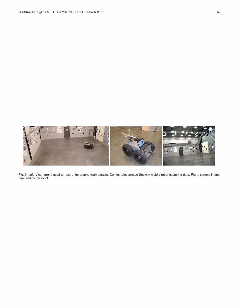
4.2.2 Vicon DatasetIn order to have a practical evaluation of the 2pt, 2.5pt and3pt algorithms, several real datasets have been collectedwith reliable ground-truth, see Fig. 9. The ground-truth datahas been obtained by conducting the experiments in a roomequipped with a Vicon motion capture system made of 22cameras. We used the Vicon data as inertial measures andscale factor in the different experiments. The sequences havebeen acquired with a perspective camera mounted eitheron teleoperated Segway mobile robot (Fig. 9) or with ahandheld system in order to have planar and 3D trajectories.In both cases the cameras are synchronized with the Viconsystem. The image resolution used is 1624 × 1234 pixels.The length of these trajectories is between 20 and 50 metersand the number of images is between 150 and 350 persequence. Robot motion speed is about 1m/s. Two differentsets have been acquired, one set showing the ground planedominantly and another set showing the walls dominantly.

We perform a comparison of the 2pt, 2.5pt and 3pt-homography with the 5pt algorithm in order to show theefficiency of the proposed methods. First, we use [33] toextract and match SIFT [34] features. The same matchedfeature point sets are used for the different algorithms andform the input to RANSAC [35] in order to select the inliers.For RANSAC we use a fixed number of 100 iterations, in allour experiments.

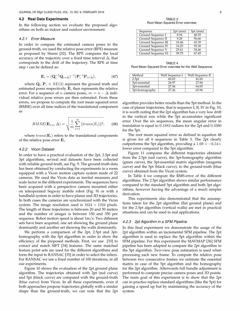
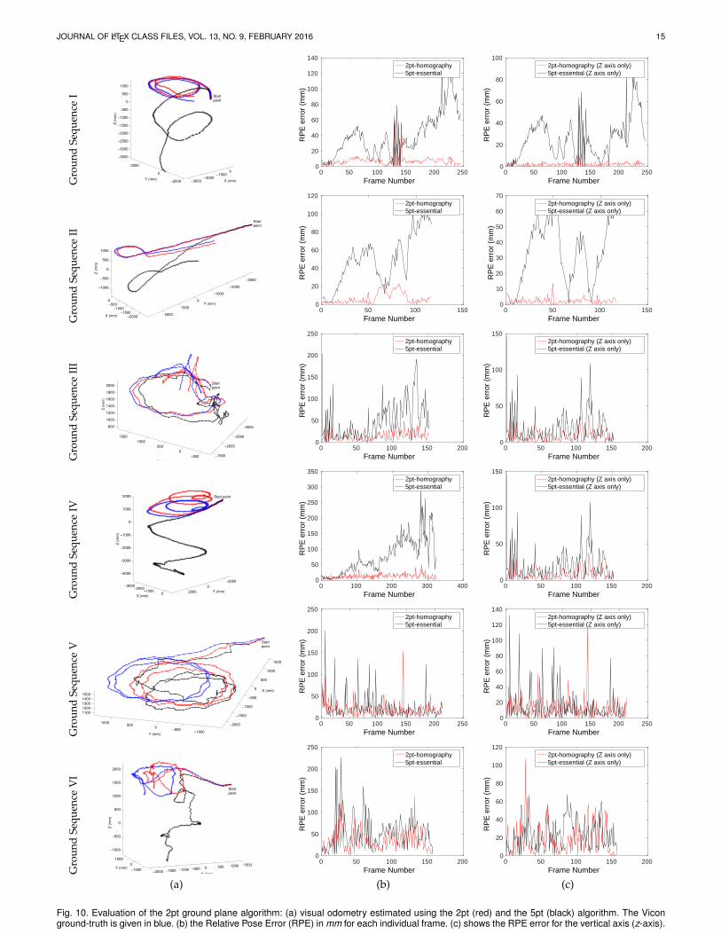
Figure 10 shows the evaluation of the 2pt ground planealgorithm. The trajectories obtained with 2pt (red curve)and 5pt (black curve) are compared with the ground-truth(blue curve) from Vicon. In all these experiments, even ifboth approaches propose trajectories globally with a similarshape than the ground-truth, we can note that the 2pt

TABLE 3Root Mean Squared Error overview.

Sequence 2pt (mm) 5pt (mm)Ground Sequence I 8.94 48.55Ground Sequence II 9.28 56.66Ground Sequence III 18.46 65.39Ground Sequence IV 14.25 93.30Ground Sequence V 25.61 34.46Ground Sequence VI 39.75 67.45

TABLE 4Root Mean Squared Error overview for the Wall Sequence.

Method Wall Sequence I Wall Sequence II2.5pt 60.65 41.605pt-essential 24.97 27.843pt-essential 27.44 64.653pt-homography 27.26 65.96

algorithm provides better results than the 5pt method. In thecase of planar trajectories, that is sequence I, II, IV in Fig. 10,it is worth noting that the 2pt algorithm has a very low driftin the vertical axis while the 5pt accumulates significanterror. Over the six sequences, the mean angular error intranslation is equal to 0.1883 radians for the 2pt and 0.3380for the 5pt.

The root mean squared error as defined in equation 48is given for all 6 sequences in Table 3. The 2pt clearlyoutperforms the 5pt algorithm, providing a 1.69 × −6.54×lower error compared to the 5pt algorithm.

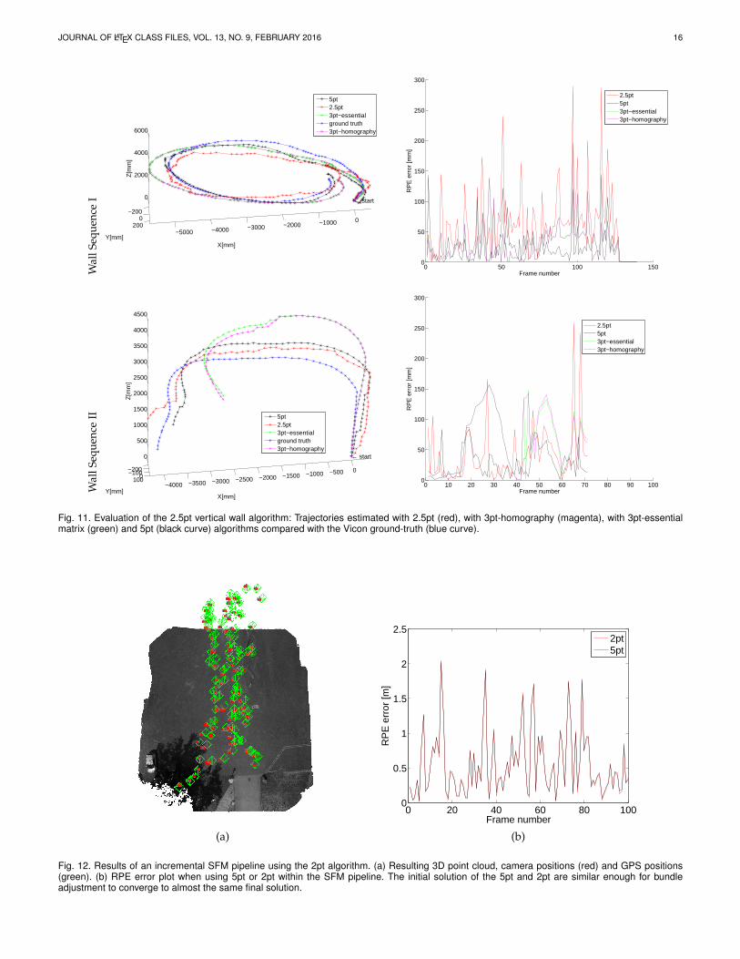
Figure 11 compares the different trajectories obtainedfrom the 2.5pt (red curve), the 3pt-homography algorithm(green curve), the 3pt-essential matrix algorithm (magentacurve) and the 5pt (black curve), to the ground-truth (bluecurve) obtained from the Vicon system.

In Table 4 we compare the RMS-error of the differentalgorithms. The 2.5pt algorithm shows similar performancecompared to the standard 5pt algorithm and both 3pt algo-rithms, however having the advantage of a much simplerderivation.

This experiments also demonstrated that the assump-tions taken for the 2pt algorithm (flat ground plane) andfor the 2.5pt algorithm (vertical walls) are met in practicalsituations and can be used in real applications.

4.2.3 2pt Algorithm in a SFM Pipeline

In this final experiment we demonstrate the usage of the2pt algorithm within an incremental SFM pipeline. The 2ptalgorithm is used to replace the 5pt algorithm within theSFM pipeline. For this experiment the MAVMAP [36] SFMpipeline has been adapted to compare the 2pt algorithm tothe 5pt algorithm. Two-view pose estimation is used whenprocessing each new frame. To compute the relative posebetween two consecutive frames we estimate the essentialmatrix in case of the 5pt algorithm and the homographyfor the 2pt algorithm. Afterwards full bundle adjustment isperformed to compute precise camera poses and 3D points.The main goal of this experiment is to show that the 2ptcan in practice replace standard algorithms (like the 5pt) forgaining a speed up but by maintaining the accuracy of thesystem.


For this experiment a UAV data set of a parking lot(denotated ParkingLot data set) is used. Images were cap-tured by a gimbal mounted camera, such that the z-axis ofthe camera aligns with the gravity direction. The datasetwas recorded at a native resolution of 24MP. The UAV wasequipped with GPS and the GPS trajectory is utilized asground truth for comparison. Figure 12 shows the results forthis experiment. Figure 12(a) shows the output of the SFMsystem, resulting 3D point cloud (densified with SURE [37]),camera positions (red) and GPS positions (green). Fig-ure 12(b) shows RPE plots for an experiment using the5pt (black) algorithm and the 2pt (red) algorithm. Bothalgorithms lead to almost identical results. The value of theremaining RPE error is mainly due to the uncertainty of theGPS measurements and expected in this form. The resultingre-projection error after bundle adjustment is 0.249px for the2pt case and 0.246px for the 5pt case, almost identical. To beclear, the reason for the identical re-projection error comesfrom bundle adjustment. This experiment demonstrates thatthe proposed 2pt algorithm can successfully replace thestandard 5pt in a SFM system seamlessly but with theadvantage of a gained speed-up.

5 CONCLUSION

In this paper we presented novel algorithms for relativepose estimation. The proposed methods differ from previ-ous algorithms by utilizing a known common direction andassumptions about the environment. This makes it possibleto derive algorithms that need less point correspondencesfor relative motion estimation as compared to state-of-the-art methods. This leads to improved RANSAC performance,which is a fundamental building block of any motion es-timation or SFM system. In our paper we show througha variety of experiments with synthetic and real data theusability of the method. In particular, the results of our realworld experiments clearly demonstrate that the assump-tions about ground plane and vertical walls really hold intypical usage scenarios. Our algorithms have successfullybeen used for indoor robot navigation as well as for 3Dreconstruction of aerial images taken from a UAV.

In addition to pure ego-motion estimation, there existsanother obvious use case for our proposed algorithms,which has not been investigated in this work. Our methodsnot only provide the motion between views but are alsoable to detect the different scene planes of the environment.In an environment consisting of vertical walls and groundplane, the proposed 2pt methods could do plane detectionmore efficient and robust as compared to the otherwise usedgeneral 4pt homography method.

APPENDIX AAN ALTERNATIVE SOLUTION TO THE 2PT HOMOG-RAPHY FORMULATION

The general homographic relation for points belonging to a3D plane and projected into two different views is definedas follows:

qj = Hqi, (49)

with qi = [xi, yi, wi]> and qj = [xj , yj , wj ]

> the projectivecoordinates of the points between the views i and j. H isgiven by:

H = R− 1

dtn>, (50)

where R and t are respectively the rotation and the trans-lation between view i and j and where d is the distancebetween the camera i and the 3D plane described by thenormal n.In our case, we assume that the camera intrinsic parametersare known and that the points qi and qj are normalized.We also consider that the attitude of the cameras for theboth views are known and that these attitude measurementshave been used to align the camera coordinate systemwith the ground plane. In this way, only the yaw angle θbetween the two views remains unknown. Similarly, sincewe consider that the ground plane constitutes the visible 3Dplane during the movement of the cameras, we can note thatn = [0, 0, 1]>.Consequently, equation(50) can be written as:

H =


0 0 1

− td

001

> , (51)

d being unknown, translation can be known only up to scale.Consequently, the camera-plane distance d is set to 1 andabsorbed by t. We then obtain:

H =


0 0 1

− txtytz

001

> ,(52)

=

cos(θ) − sin(θ) −txsin(θ) cos(θ) −ty

0 0 1− tz

. (53)

If 1 − tz 6= 0, then the homography can be scaled, bydeviding H by 1− tz , which results in:

H =

cos(θ)1−tz − sin(θ)

1−tz − tx1−tz

sin(θ)1−tz

cos(θ)1−tz − ty

1−tz0 0 1

. (54)

In a general manner, this homography can be written as

H =

h1 −h2 h3

h2 h1 h4

0 0 1

. (55)

The problem consists then in estimating this homogra-phy. In this way, we consider the following relation:

qj ×Hqi = 0, (56)

where × denotes the cross product. In our case, we obtain: xjyjwj

× h1 −h2 h3

h2 h1 h4

0 0 1

xiyiwi

= 0, (57)

wiyj − wj(h2xi + h1yi + h4wi)−wixj + wj(h1xi + h2yi + h3wi)

xj(h2xi + h1yi + h4wi)− yj(h1xi + h2yi + h3wi)

= 0.

(58)


The third equation being a linear combination of the twoothers, we only consider the two first lines of the previoussystem and obtain:[

wiyj − wjh2xi − wjh1yi − wjh4wi−wixj + wjh1xi − wjh2yi − wjh3wi)

]= 0, (59)

which can be finally rewritten as

[−wjyi −wjxi 0 −wjwiwjxi −wjyi wjwi 0

]h1

h2

h3

h4

=

[−wiyjwixj

].

(60)We can observe that two points are sufficient in order toestimate the hl, l = {1, 2, 3, 4} elements and that the systemcan be easily extended to n points in order to obtain an overdetermined system. This possibility is then very interestingbecause it permits to apply a RANSAC algorithm in orderto reject the outliers.

Once the hl, l = {1, 2, 3, 4} estimated, we are thenable to evaluate the motion parameters, i.e., θ, tx, ty andtz . By identification between (55) and (54), we know thath1 = cos(θ)

1−tz and h2 = sin(θ)1−tz . Then, if h1 6= 0, we have

tan(θ) = h2

h1and finally θ = arctan(h2

h1). Due to the

periodicity of arctan two solutions arises, θ and θ + π. Ifh1 = 0, then θ = ±π2 .

Knowing the angle yaw θ between the two views and ifh1 6= 0, we then have tz = 1− cos(θ)

h1. If h1 = 0, then θ = ±π2

and we can use the relation h2 = sin(θ)1−tz , to obtain tz = 1± 1

h2.

Consequently, we can deduce the two remaining translationparameters tx = h3(tz − 1) and ty = h4(tz − 1).

ACKNOWLEDGMENTS

This work has been partially supported by Project ANRBlanc International DrAACaR-ANR-11-IS03-0003 and aGoogle Award. We also thank the anonymous reviewers fortheir useful discussions and constructive comments.

REFERENCES

[1] R. Hartley and A. Zisserman, Multiple View Geometry in ComputerVision, 2nd ed. Cambridge University Press, ISBN: 0521540518,2004.

[2] D. Nister, “An efficient solution to the five-point relative poseproblem,” IEEE Trans. Pattern Anal. Mach. Intell., vol. 26, no. 6,pp. 756–777, 2004.

[3] F. Fraundorfer, P. Tanskanen, and M. Pollefeys, “A minimal casesolution to the calibrated relative pose problem for the case oftwo known orientation angles,” in ECCV (4), ser. Lecture Notesin Computer Science, K. Daniilidis, P. Maragos, and N. Paragios,Eds., vol. 6314. Springer, 2010, pp. 269–282.

[4] D. Scaramuzza, “1-point-ransac structure from motion for vehicle-mounted cameras by exploiting non-holonomic constraints,” Inter-national Journal of Computer Vision, vol. 95, no. 1, pp. 74–85, 2011.

[5] L. Kneip, A. Martinelli, S. Weiss, D. Scaramuzza, and R. Siegwart,“Closed-form solution for absolute scale velocity determinationcombining inertial measurements and a single feature correspon-dence,” in IEEE International Conference on Robotics and Automation,ICRA 2011, Shanghai, China, 9-13 May 2011, 2011, pp. 4546–4553.

[6] T. Vieville, E. Clergue, and P. D. S. Facao, “Computation of ego-motion and structure from visual and inertial sensors using thevertical cue,” in Computer Vision, 1993. Proceedings., Fourth Interna-tional Conference on. IEEE, 1993, pp. 591–598.

[7] P. Corke, “An inertial and visual sensing system for a smallautonomous helicopter,” Journal of Robotic Systems, vol. 21, no. 2,pp. 43–51, 2004.

[8] J. Lobo and J. Dias, “Vision and inertial sensor cooperation usinggravity as a vertical reference,” IEEE Trans. Pattern Anal. Mach.Intell., vol. 25, no. 12, pp. 1597–1608, 2003.

[9] S. Weiss and R. Siegwart, “Real-time metric state estimationfor modular vision-inertial systems,” in Robotics and Automation(ICRA), 2011 IEEE International Conference on. IEEE, 2011, pp.4531–4537.

[10] J. Domke and Y. Aloimonos, “Integration of visual and inertialinformation for egomotion: a stochastic approach,” in Robotics andAutomation, 2006. ICRA 2006. Proceedings 2006 IEEE InternationalConference on. IEEE, 2006, pp. 2053–2059.

[11] J.-C. Bazin, H. Li, I. S. Kweon, C. Demonceaux, P. Vasseur, andK. Ikeuchi, “A branch-and-bound approach to correspondenceand grouping problems,” IEEE Transactions on Pattern Analysis andMachine Intelligence, vol. 35, no. 7, pp. 1565–1576, 2013.

[12] O. Oreifej, N. da Vitoria Lobo, and M. Shah, “Horizon constraintfor unambiguous uav navigation in planar scenes,” in IEEE Inter-national Conference on Robotics and Automation, ICRA 2011, Shanghai,China, 9-13 May 2011, 2011, pp. 1159–1165.

[13] D. Ortin and J. Montiel, “Indoor robot motion based on monocularimages,” Robotica, vol. 19, no. 3, pp. 331–342, 2001.

[14] C. Troiani, A. Martinelli, C. Laugier, and D. Scaramuzza, “1-point-based monocular motion estimation for computationally-limitedmicro aerial vehicles,” in Mobile Robots (ECMR), 2013 EuropeanConference on. IEEE, 2013, pp. 13–18.

[15] J.-C. Bazin, C. Demonceaux, P. Vasseur, and I. Kweon, “Rotationestimation and vanishing point extraction by omnidirectional vi-sion in urban environment,” The International Journal of RoboticsResearch, vol. 31, no. 1, pp. 63–81, 2012.

[16] B. Li, L. Heng, G. H. Lee, and M. Pollefeys, “A 4-point algorithmfor relative pose estimation of a calibrated camera with a knownrelative rotation angle,” in Proc. IEEE/RSJ Int. Conf. on IntelligentRobots and Systems, IROS 2013, Tokyo, Japan, 2013.

[17] M. Kalantari, A. Hashemi, F. Jung, and J.-P. Guedon, “A newsolution to the relative orientation problem using only 3 pointsand the vertical direction,” Journal of Mathematical Imaging andVision, vol. 39, no. 3, pp. 259–268, 2011.

[18] O. Naroditsky, X. S. Zhou, J. H. Gallier, S. I. Roumeliotis, andK. Daniilidis, “Two efficient solutions for visual odometry usingdirectional correspondence,” IEEE Trans. Pattern Anal. Mach. Intell.,vol. 34, no. 4, pp. 818–824, 2012.

[19] C. Troiani, A. Martinelli, C. Laugier, and D. Scaramuzza, “2-point-based outlier rejection for camera-imu systems with appli-cations to micro aerial vehicles,” in IEEE International Conferenceon Robotics and Automation (ICRA), Hong Kong, 2014., 2014.

[20] J.-C. Bazin, C. Demonceaux, P. Vasseur, and I. Kweon, “Motionestimation by decoupling rotation and translation in catadioptricvision,” Computer Vision and Image Understanding, vol. 114, no. 2,pp. 254–273, 2010.

[21] A. Martinelli, “Closed-form solution of visual-inertial structurefrom motion,” International Journal of Computer Vision, vol. 106,no. 2, pp. 138–152, 2014.

[22] G. H. Lee, F. Fraundorfer, and M. Pollefeys, “Mav visual slam withplane constraint,” in ICRA. IEEE, 2011, pp. 3139–3144.

[23] C. Troiani, S. Al Zanati, and A. Martinelli, “A 3 Points Vision BasedApproach for MAV Localization in GPS Denied Environments,”in 6th European Conference on Mobile Robots, Barcelona, Spain, 2013.[Online]. Available: http://hal.inria.fr/hal-00909613

[24] J. M. Coughlan and A. L. Yuille, “Manhattan world: Compassdirection from a single image by bayesian inference,” in InternationConference on Computer Vision, 1999, pp. 941–947.

[25] Y. Furukawa, B. Curless, S. M. Seitz, and R. Szeliski, “Manhattan-world stereo,” in IEEE Computer Society Conference on ComputerVision and Pattern Recognition (CVPR). Miami, FL: IEEE, June2009, pp. 1422–1429.

[26] ——, “Reconstructing building interiors from images.” in Proc. ofthe International Conference on Computer Vision (ICCV), 2009, pp.80–87.

[27] D. C. Lee, M. Hebert, and T. Kanade, “Geometric reasoning forsingle image structure recovery,” in IEEE Computer Society Confer-ence on Computer Vision and Pattern Recognition (CVPR), 2009, pp.2136–2143.


[28] O. Saurer, F. Fraundorfer, and M. Pollefeys, “Homography basedvisual odometry with known vertical direction and weak manhat-tan world assumption,” in Vicomor Workshop at IROS, 2012.

[29] O. Saurer, P. Vasseur, C. Demonceaux, and F. Fraundorfer, “Ahomography formulation to the 3pt plus a common directionrelative pose problem,” in Computer vision–ACCV. Springer, 2014.

[30] D. A. Cox, J. Little, and D. O’Shea, Ideals, Varieties, and Algorithms:An Introduction to Computational Algebraic Geometry and Commuta-tive Algebra, 3/e (Undergraduate Texts in Mathematics). Secaucus,NJ, USA: Springer-Verlag New York, Inc., 2007.

[31] Z. Kukelova, M. Bujnak, and T. Pajdla, “Automatic generator ofminimal problem solvers,” in Computer Vision - ECCV 2008, 10thEuropean Conference on Computer Vision, Marseille, France, October12-18, 2008, Proceedings, Part III, ser. Lecture Notes in ComputerScience, D. A. Forsyth, P. H. S. Torr, and A. Zisserman, Eds., vol.5304. Springer, 2008, pp. 302–315.

[32] J. Sturm, N. Engelhard, F. Endres, W. Burgard, and D. Cremers, “Abenchmark for the evaluation of rgb-d slam systems,” in Proc. ofthe International Conference on Intelligent Robot Systems (IROS), Oct.2012.

[33] A. Vedaldi and B. Fulkerson, “VLFeat: An open and portablelibrary of computer vision algorithms,” http://www.vlfeat.org/,2008.

[34] D. G. Lowe, “Distinctive image features from scale-invariant key-points,” in International Journal on Computer Vision (IJCV), vol. 60,no. 2, 2004, pp. 91–110.

[35] M. A. Fischler and R. C. Bolles, “Random sample consensus: Aparadigm for model fitting with applications to image analysisand automated cartography,” Commun. ACM, vol. 24, no. 6, pp.381–395, Jun. 1981.

[36] J. L. Schonberger, F. Fraundorfer, and J.-M. Frahm,“Structure-from-motion for mav image sequence analysiswith photogrammetric applications,” ISPRS - InternationalArchives of the Photogrammetry, Remote Sensing andSpatial Information Sciences, vol. XL-3, pp. 305–312, 2014.[Online]. Available: http://www.int-arch-photogramm-remote-sens-spatial-inf-sci.net/XL-3/305/2014/

[37] D. F. M. Rothermel, K. Wenzel and N. Haala, “Sure: Photogram-metric surface reconstruction from imagery,” in Proceedings LC3DWorkshop, 2014.

Olivier Saurer received his MSc in computerscience from ETH Zurich in 2009. He is cur-rently a graduate student at ETH Zurich in theComputer Vision and Geometry Group. His re-search interests include sparse and dense re-construction methods for omnidirectional andmonoclular vision and its application on chal-lenging datasets.

Pascal Vasseur received the M.S. degree inSystem Control from Universite de Technologiede Compiegne (France) in 1995 and his Ph.D.in Automatic Control from Universite de PicardieJules Verne (France) in 1998. He was associateprofessor at the Universite de Picardie JulesVerne in Amiens between 1999 and 2010. He isnow a full professor at the Universite de Rouenand is member of LITIS laboratory. His researchinterests are computer vision and its applicationsto mobile and aerial robots.

Remi Boutteau received his engineeringdiploma from the Ecole des Mines de Douaiand his MSc degree in computer science andengineering from the University of Science andTechnology of Lille (USTL) in 2006. In 2010, hereceived his PhD degree from the University ofRouen for studies related to computer vision,panoramic vision obtained by catadioptricsensors, and 3D reconstruction algorithmsdedicated to omnidirectional vision. After hisPhD, he has joined the ESIGELEC engineering

school as a lecturer in embedded systems, and the ”Instrumentation,Computer Sciences and Systems” research team in the IRSEEMLaboratory. His research interests include computer vision, structurefrom motion, visual odometry and omnidirectional vision dedicated toautonomous vehicles.

Cedric Demonceaux received the M.S. degreein Mathematics in 2001 and the PhD degreein Image Processing from the Universite de Pi-cardie Jules Verne (UPJV), France, in 2004.In 2005, he became associate professor atMIS-UPJV. From 2010 to 2014, he has beenan CNRS-Higher Education chair at Le2I UMRCNRS, Universite de Bourgogne. Since 2014, heis full Professor at the University of Burgundy.His research interests are in image processing,computer vision and robotics.

Marc Pollefeys is a full professor in the Dept.of Computer Science of ETH Zurich since 2007.Before that he was on the faculty at the Univer-sity of North Carolina at Chapel Hill. He obtainedhis PhD from the KU Leuven in Belgium in 1999.His main area of research is computer vision, buthe is also active in robotics, machine learningand computer graphics. Dr. Pollefeys has re-ceived several prizes for his research, includinga Marr prize, an NSF CAREER award, a PackardFellowship and a European Research Council

Grant. He is the author or co-author of more than 250 peer-reviewedpublications. He was the general chair of ECCV 2014 in Zurich andprogram chair of CVPR 2009. He is a fellow of the IEEE.

Friedrich Fraundorfer is Assistant Professor atGraz University of Technology, Austria. He re-ceived the Ph.D. degree in computer sciencefrom TU Graz in 2006. He had post-doc staysat the University of Kentucky, at the Universityof North Carolina at Chapel Hill, at ETH Zurichand acted as Deputy Director of the Chair ofRemote Sensing Technology at the TechnischeUniversitat Munchen from 2012 to 2014. Hismain research areas are 3D computer vision androbot vision.


Side

way

sm

otio

n

Noise in Pixel0 0.1 0.2 0.3 0.4 0.5 0.6 0.7 0.8 0.9 1

Rot

atio

n E

rror

in D

egre

e

0

1

2

3

4

5

6

7

85-Quantile

5pt-essential4pt-homography3pt-essential2pt-homography

Noise in Pixel0 0.1 0.2 0.3 0.4 0.5 0.6 0.7 0.8 0.9 1

Tra

nsla

tion

Err

or in

Deg

ree

0

10

20

30

40

50

60

705-Quantile


Forw

ard

mot

ion

Noise in Pixel0 0.1 0.2 0.3 0.4 0.5 0.6 0.7 0.8 0.9 1

Rot

atio

n E

rror

in D

egre

e

0

0.5

1

1.5

2

2.5

3

3.55-Quantile


Noise in Pixel0 0.1 0.2 0.3 0.4 0.5 0.6 0.7 0.8 0.9 1

Tra

nsla

tion

Err

or in

Deg

ree

0

5

10

15

20

255-Quantile


Fig. 3. Evaluation of the 2 point algorithm under sideways and forward motion with varying image noise.

Side

way

sm

otio

n

Rotation Noise in Degree (Pitch)0 0.1 0.2 0.3 0.4 0.5 0.6 0.7 0.8 0.9 1

Rot

atio

n E

rror

in D

egre

e

0

1

2

3

4

5

6

75-Quantile


Rotation Noise in Degree (Roll)0 0.1 0.2 0.3 0.4 0.5 0.6 0.7 0.8 0.9 1

Rot

atio

n E

rror

in D

egre

e

0

1

2

3

4

5

6

75-Quantile



Tra

nsla

tion

Err

or in

Deg

ree

0

10

20

30

40

50

60

705-Quantile



Tra

nsla

tion

Err

or in

Deg

ree

0

10

20

30

40

50

60

705-Quantile


Forw

ard

mot

ion


Rot

atio

n E

rror

in D

egre

e

0

0.5

1

1.5

2

2.5

3

3.55-Quantile



Rot

atio

n E

rror

in D

egre

e

0

0.5

1

1.5

2

2.5

3

3.55-Quantile



Tra

nsla

tion

Err

or in

Deg

ree

0

5

10

15

20

255-Quantile



Tra

nsla

tion

Err

or in

Deg

ree

0

5

10

15

20

255-Quantile


Fig. 4. Evaluation of the 2pt algorithm under different IMU noise and constant image noise of 0.5 pixel standard deviation. First row, sidewaysmotion, second row forward motion.

Side

way

sm

otio

n

Noise in Pixel0 0.1 0.2 0.3 0.4 0.5 0.6 0.7 0.8 0.9 1

Rot

atio

n E

rror

in D

egre

e

0

0.5

1

1.5

2

2.5

3

3.5

4

4.5

55-Quantile

5pt-essential4pt-homography3pt-essential2.5pt-homography

Noise in Pixel0 0.1 0.2 0.3 0.4 0.5 0.6 0.7 0.8 0.9 1

Tra

nsla

tion

Err

or in

Deg

ree

0

5

10

15

20

255-Quantile


Forw

ard

mot

ion

Noise in Pixel0 0.1 0.2 0.3 0.4 0.5 0.6 0.7 0.8 0.9 1

Rot

atio

n E

rror

in D

egre

e

0

0.2

0.4

0.6

0.8

1

1.2

1.45-Quantile


Noise in Pixel0 0.1 0.2 0.3 0.4 0.5 0.6 0.7 0.8 0.9 1

Tra

nsla

tion

Err

or in

Deg

ree

0

1

2

3

4

5

6

7

8

9

105-Quantile


Fig. 5. Evaluation of the 2.5pt algorithm under sideways and forward motion with varying image noise.


Side

way

sm

otio

n


Rot

atio

n E

rror

in D

egre

e

0.8

1

1.2

1.4

1.6

1.8

2

2.2

2.4

2.65-Quantile



Rot

atio

n E

rror

in D

egre

e

0.4

0.6

0.8

1

1.2

1.4

1.6

1.8

2

2.25-Quantile



Tra

nsla

tion

Err

or in

Deg

ree

1

2

3

4

5

6

7

8

9

10

115-Quantile



Tra

nsla

tion

Err

or in

Deg

ree

0

1

2

3

4

5

6

7

85-Quantile


Forw

ard

mot

ion


Rot

atio

n E

rror

in D

egre

e

0.2

0.3

0.4

0.5

0.6

0.7

0.8

0.9

15-Quantile



Rot

atio

n E

rror

in D

egre

e

0.3

0.4

0.5

0.6

0.7

0.8

0.9

1

1.1

1.2

1.35-Quantile



Tra

nsla

tion

Err

or in

Deg

ree

2

3

4

5

6

7

85-Quantile



Tra

nsla

tion

Err

or in

Deg

ree

2

3

4

5

6

7

8

95-Quantile


Fig. 6. Evaluation of the 2.5pt algorithm under IMU noise and constant image noise of 0.5 pixel standard deviation. First row sideways motion,second row forward motion.

Side

way

sm

otio

n

Noise in Pixel0 0.1 0.2 0.3 0.4 0.5 0.6 0.7 0.8 0.9 1

Rot

atio

n E

rror

in D

egre

e

0

0.05

0.1

0.15

0.2

0.25

0.35-Quantile

5pt-essential3pt-essential3pt-homography

Noise in Pixel0 0.1 0.2 0.3 0.4 0.5 0.6 0.7 0.8 0.9 1

Tra

nsla

tion

Err

or in

Deg

ree

0

0.1

0.2

0.3

0.4

0.5

0.6

0.7

0.8

0.9

15-Quantile


Forw

ard

mot

ion

Noise in Pixel0 0.1 0.2 0.3 0.4 0.5 0.6 0.7 0.8 0.9 1

Rot

atio

n E

rror

in D

egre

e

0

0.05

0.1

0.15

0.2

0.25

0.3

0.355-Quantile


Noise in Pixel0 0.1 0.2 0.3 0.4 0.5 0.6 0.7 0.8 0.9 1

Tra

nsla

tion

Err

or in

Deg

ree

0

0.2

0.4

0.6

0.8

1

1.2

1.4

1.65-Quantile


Fig. 7. Evaluation of the 3pt-homography algorithm under sideways and forward motion with varying image noise.

Side

way

sm

otio

n


Rot

atio

n E

rror

in D

egre

e

0

0.05

0.1

0.15

0.2

0.25

0.3

0.35

0.45-Quantile



Rot

atio

n E

rror

in D

egre

e

0

0.05

0.1

0.15

0.2

0.25

0.3

0.35

0.45-Quantile



Tra

nsla

tion

Err

or in

Deg

ree

0.1

0.2

0.3

0.4

0.5

0.6

0.75-Quantile



Tra

nsla

tion

Err

or in

Deg

ree

0

0.5

1

1.5

2

2.55-Quantile


Forw

ard

mot

ion


Rot

atio

n E

rror

in D

egre

e

0

0.05

0.1

0.15

0.2

0.25

0.3

0.35

0.45-Quantile



Rot

atio

n E

rror

in D

egre

e

0

0.05

0.1

0.15

0.2

0.25

0.3

0.355-Quantile



Tra

nsla

tion

Err

or in

Deg

ree

0.1

0.2

0.3

0.4

0.5

0.6

0.75-Quantile



Tra

nsla

tion

Err

or in

Deg

ree

0

0.2

0.4

0.6

0.8

1

1.2

1.4

1.65-Quantile


Fig. 8. Evaluation of the 3pt-homography algorithm under different IMU noise and constant image noise of 0.5 pixel standard deviation. First row:sideways motion of the camera with varying pitch angle (left) and varying roll angle (right). Second row: forward motion of the camera with varyingpitch angle (left) and varying roll angle (right).


Fig. 9. Left, Vicon arena used to record the ground-truth dataset. Center, teleoperated Segway mobile robot capturing data. Right, sample imagecaptured by the robot.


Gro

und

Sequ

ence

I

−3000−2000

−10000

−2000

0

2000

−3500

−3000

−2500

−2000

−1500

−1000

−500

0

500

1000

X (mm)Y (mm)

Z (

mm

)

Startpoint

Frame Number0 50 100 150 200 250

RP

E e

rror

(m

m)

0

20

40

60

80

100

120

1402pt-homography5pt-essential

Frame Number0 50 100 150 200 250

RP

E e

rror

(m

m)

0

20

40

60

80

1002pt-homography (Z axis only)5pt-essential (Z axis only)

Gro

und

Sequ

ence

II

−2000−1500

−1000−5000

−3000

−2000

−1000

0

1000

2000

−1000

−500

0

500

1000

Y (mm)

X (mm)

Z (

mm

)

Startpoint

Frame Number0 50 100 150

RP

E e

rror

(m

m)

0

20

40

60

80

100


Frame Number0 50 100 150

RP

E e

rror

(m

m)

0

10

20

30

40

50

60


Gro

und

Sequ

ence

III

−3000

−2500

−2000

−1500−500

0

500

1000

1500

800

1000

1200

1400

1600

1800

2000

X (mm)Y (mm)

Z (

mm

)

Startpoint

Frame Number0 50 100 150 200

RP

E e

rror

(m

m)

0

50

100

150

200


Frame Number0 50 100 150 200

RP

E e

rror

(m

m)

0

50

100


Gro

und

Sequ

ence

IV

−3000−2000

−10000

−2000

0

2000

−4000

−3000

−2000

−1000

0

1000

2000

Y (mm)X (mm)

Z (

mm

)

Start point

Frame Number0 100 200 300 400

RP

E e

rror

(m

m)

0

50

100

150

200

250

300


Frame Number0 50 100 150 200

RP

E e

rror

(m

m)

0

50

100


Gro

und

Sequ

ence

V

−2000

−1500

−1000

−500

0

500

1000

1500

−1000−500

0500

1000

1100

1200

1300

1400

1500X (mm)

Y (mm)

Z (

mm

)

Startpoint

Frame Number0 50 100 150 200 250

RP

E e

rror

(m

m)

0

50

100

150

200


Frame Number0 50 100 150 200 250

RP

E e

rror

(m

m)

0

20

40

60

80

100

120


Gro

und

Sequ

ence

VI

−2000 −1500 −1000 −500 0 500 1000 1500

−1000

0

1000

−1000

−500

0

500

1000

1500

2000

X (mm)

Y (mm)

Z (

mm

)

Startpoint

Frame Number0 50 100 150 200

RP

E e

rror

(m

m)

0

50

100

150

200


Frame Number0 50 100 150 200

RP

E e

rror

(m

m)

0

20

40

60

80

100


(a) (b) (c)

Fig. 10. Evaluation of the 2pt ground plane algorithm: (a) visual odometry estimated using the 2pt (red) and the 5pt (black) algorithm. The Viconground-truth is given in blue. (b) the Relative Pose Error (RPE) in mm for each individual frame. (c) shows the RPE error for the vertical axis (z-axis).


Wal

lSeq

uenc

eI

−5000 −4000 −3000 −2000 −1000 0−200

0200

0

2000

4000

6000

← start

X[mm]

Z[m

m]

Y[mm]

5pt2.5pt3pt−essentialground truth3pt−homography

0 50 100 1500

50

100

150

200

250

300

Frame number

RP

E e

rror

[mm

]

2.5pt5pt3pt−essential3pt−homography

Wal

lSeq

uenc

eII

−4000 −3500 −3000 −2500 −2000 −1500 −1000 −500 0−200−1000100

0

500

1000

1500

2000

2500

3000

3500

4000

4500

← start

X[mm]

Z[m

m]

Y[mm]

5pt2.5pt3pt−essentialground truth3pt−homography

0 10 20 30 40 50 60 70 80 90 1000

50

100

150

200

250

300

Frame number

RP

E e

rror

[mm

]

2.5pt5pt3pt−essential3pt−homography

Fig. 11. Evaluation of the 2.5pt vertical wall algorithm: Trajectories estimated with 2.5pt (red), with 3pt-homography (magenta), with 3pt-essentialmatrix (green) and 5pt (black curve) algorithms compared with the Vicon ground-truth (blue curve).

0 20 40 60 80 1000

0.5

1

1.5

2

2.5

Frame number

RP

E e

rror

[m]

2pt5pt

(a) (b)

Fig. 12. Results of an incremental SFM pipeline using the 2pt algorithm. (a) Resulting 3D point cloud, camera positions (red) and GPS positions(green). (b) RPE error plot when using 5pt or 2pt within the SFM pipeline. The initial solution of the 5pt and 2pt are similar enough for bundleadjustment to converge to almost the same final solution.

Documents

JOURNAL OF LA Homography Based Egomotion Estimation with …people.inf.ethz.ch/saurero/publications/saurer_2016_homography... · JOURNAL OF LATEX CLASS FILES, VOL. 13, NO. 9, FEBRUARY