Embed Size (px)
Citation preview
Homography from two orientation- and scale-covariant features
Daniel Barath1,2 Zuzana Kukelova1
1 VRG, Department of Cybernetics, Czech Technical University in Prague, Czech Republic2 Machine Perception Research Laboratory, MTA SZTAKI, Budapest, Hungary
Abstract
This paper proposes a geometric interpretation of the an-
gles and scales which the orientation- and scale-covariant
feature detectors, e.g. SIFT, provide. Two new general con-
straints are derived on the scales and rotations which can be
used in any geometric model estimation tasks. Using these
formulas, two new constraints on homography estimation
are introduced. Exploiting the derived equations, a solver
for estimating the homography from the minimal number of
two correspondences is proposed. Also, it is shown how
the normalization of the point correspondences affects the
rotation and scale parameters, thus achieving numerically
stable results. Due to requiring merely two feature pairs,
robust estimators, e.g. RANSAC, do significantly fewer it-
erations than by using the four-point algorithm. When us-
ing covariant features, e.g. SIFT, the information about the
scale and orientation is given at no cost. The proposed ho-
mography estimation method is tested in a synthetic envi-
ronment and on publicly available real-world datasets.
1. Introduction
This paper addresses the problem of interpreting, in a ge-
ometrically justifiable manner, the rotation and scale which
the orientation- and scale-covariant feature detectors, e.g.
SIFT [22] or SURF [10], provide. Then, by exploiting
these new constraints, we involve all the obtained param-
eters of the SIFT features (i.e. the point coordinates, angle,
and scale) into the homography estimation procedure. In
particular, we are interested in the minimal case, to estimate
a homography from solely two correspondences.
Nowadays, a number of algorithms exist for estimating
or approximating geometric models, e.g. homographies, us-
ing affine-covariant features. A technique, proposed by Per-
doch et al. [29], approximates the epipolar geometry from
one or two affine correspondences by converting them to
point pairs. Bentolila and Francos [11] proposed a solution
for estimating the fundamental matrix using three affine fea-
tures. Raposo et al. [32, 31] and Barath et al. [6] showed that
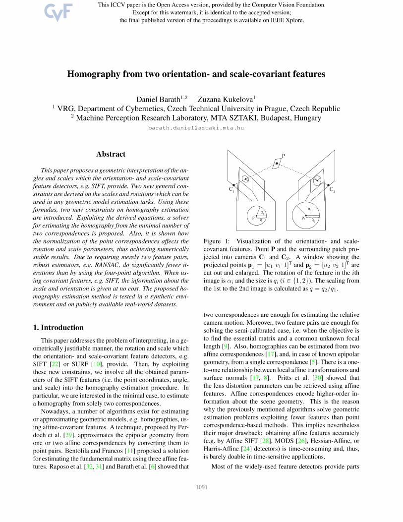
C1
C2
P
α2
q2
p2
α1
q1
p1
Figure 1: Visualization of the orientation- and scale-
covariant features. Point P and the surrounding patch pro-
jected into cameras C1 and C2. A window showing the
projected points p1 = [u1 v1 1]T and p2 = [u2 v2 1]T are
cut out and enlarged. The rotation of the feature in the ithimage is αi and the size is qi (i ∈ {1, 2}). The scaling from
the 1st to the 2nd image is calculated as q = q2/q1.
two correspondences are enough for estimating the relative
camera motion. Moreover, two feature pairs are enough for
solving the semi-calibrated case, i.e. when the objective is
to find the essential matrix and a common unknown focal
length [9]. Also, homographies can be estimated from two
affine correspondences [17], and, in case of known epipolar
geometry, from a single correspondence [5]. There is a one-
to-one relationship between local affine transformations and
surface normals [17, 8]. Pritts et al. [30] showed that
the lens distortion parameters can be retrieved using affine
features. Affine correspondences encode higher-order in-
formation about the scene geometry. This is the reason
why the previously mentioned algorithms solve geometric
estimation problems exploiting fewer features than point
correspondence-based methods. This implies nevertheless
their major drawback: obtaining affine features accurately
(e.g. by Affine SIFT [28], MODS [26], Hessian-Affine, or
Harris-Affine [24] detectors) is time-consuming and, thus,
is barely doable in time-sensitive applications.
Most of the widely-used feature detectors provide parts
11091
of the affine feature. For instance, there are detectors ob-
taining oriented features, e.g. ORB [33], or there are ones
providing also the scales, e.g. SIFT [22] or SURF [10].
Exploiting this additional information is a well-known ap-
proach in, for example, wide-baseline matching [23, 26].
Yet, the first papers [1, 2, 3, 25, 4] involving them into geo-
metric model estimation were published just in the last few
years. In [25], the feature orientations are involved directly
in the essential matrix estimation. In [1], the fundamental
matrix is assumed to be a priori known and an algorithm is
proposed for approximating a homography exploiting the
rotations and scales of two SIFT correspondences. The
approximative nature comes from the assumption that the
scales along the axes are equal to the SIFT scale and the
shear is zero. In general, these assumptions do not hold.
The method of [2] approximates the fundamental matrix
by enforcing the geometric constraints of affine correspon-
dences on the epipolar lines. Nevertheless, due to using the
same affine model as in [1], the estimated epipolar geometry
is solely an approximation. In [3], a two-step procedure is
proposed for estimating the epipolar geometry. First, a ho-
mography is obtained from three oriented features. Finally,
the fundamental matrix is retrieved from the homography
and two additional correspondences. Even though this tech-
nique considers the scales and shear as unknowns, thus es-
timating the epipolar geometry instead of approximating it,
the proposed decomposition of the affine matrix is not jus-
tified theoretically. Therefore, the geometric interpretation
of the feature rotations is not provably valid. A recently
published paper [4] proposes a way of recovering full affine
correspondences from the feature rotation, scale, and the
fundamental matrix. Applying this method, a homography
is estimated from a single correspondence in case of known
epipolar geometry. Still, the decomposition of the affine
matrix is ad hoc, and is, therefore, not a provably valid in-
terpretation of the SIFT rotations and scales. Moreover, in
practice, the assumption of the known epipolar geometry
restricts the applicability of the method.
The contributions of this paper are: (i) we provide a ge-
ometrically valid way of interpreting orientation- and scale-
covariant features approaching the problem by differential
geometry. (ii) Building on the derived formulas, we propose
two general constraints which hold for covariant features.
(iii) These constraints are then used to derive two new for-
mulas for homography estimation and (iv), based on these
equations, a solver is proposed for estimating a homogra-
phy matrix from two orientation- and scale-covariant fea-
ture correspondences. This additional information, i.e. the
scale and rotation, is given at no cost when using most of
the widely-used feature detectors, e.g. SIFT or SURF. It is
validated both in a synthetic environment and on more than
10 000 publicly available real image pairs that the solver ac-
curately recovers the homography matrix. Benefiting from
the number of correspondences required, robust estimation,
e.g. by GC-RANSAC [7], is two orders of magnitude faster
than by combining it with the standard techniques, e.g. four-
point algorithm [16].
2. Theoretical background
Affine correspondence (p1,p2,A) is a triplet, where p1 =[u1 v1 1]T and p2 = [u2 v2 1]T are a corresponding homo-
geneous point pair in two images and A is a 2 × 2 linear
transformation which is called local affine transformation.
Its elements in a row-major order are: a1, a2, a3, and a4. To
define A, we use the definition provided in [27] as it is given
as the first-order Taylor-approximation of the 3D → 2D
projection functions. For perspective cameras, the formula
for A is the first-order approximation of the related homog-
raphy matrix as follows:
a1 = ∂u2
∂u1
= h1−h7u2
s, a2 = ∂u2
∂v1
= h2−h8u2
s,
a3 = ∂v2
∂u1
= h4−h7v2
s, a4 = ∂v2
∂v1= h5−h8v2
s,
(1)
where ui and vi are the directions in the ith image (i ∈{1, 2}) and s = u1h7 + v1h8 + h9 is the projective depth.
The elements of H in a row-major order are: h1, h2, ..., h9.
The relationship of an affine correspondence and a homog-
raphy is described by six linear equations. Since an affine
correspondence involves a point pair, the well-known equa-
tions (from Hp1 ∼ p2) hold [16]. They are as follows:
u1h1 + v1h2 + h3 − u1u2h7 − v1u2h8 − u2h9 = 0,
u1h4 + v1h5 + h6 − u1v2h7 − v1v2h8 − v2h9 = 0.(2)
After re-arranging (1), four additional linear constraints are
obtained from A which are the following.
h1 − (u2 + a1u1)h7 − a1v1h8 − a1h9 = 0,
h2 − (u2 + a2v1)h8 − a2u1h7 − a2h9 = 0,
h4 − (v2 + a3u1)h7 − a3v1h8 − a3h9 = 0,
h5 − (v2 + a4v1)h8 − a4u1h7 − a4h9 = 0.
(3)
Consequently, an affine correspondence provides six linear
equations for the elements of the related homography.
3. Affine transformation model
In this section, the interpretation of the feature scales
and rotations are discussed. Two new constraints that re-
late the elements of the affine transformation to the feature
scale and rotation are derived. These constraints are gen-
eral, and they can be used for estimating different geometric
models, e.g. homographies or fundamental matrices, using
orientation- and scale-covariant features. In this paper, the
two constraints are used to derive a solver for homography
estimation from two correspondences. For the sake of sim-
plicity, we use SIFT as an alias for all the orientation- and
scale-covariant detectors. The formulas hold for all of them.
21092
3.1. Interpretation of the SIFT output
Reflecting the fact that we are given a scale qi ∈ R
and rotation αi ∈ [0, 2π) independently in each image
(i ∈ {1, 2}; see Fig. 1), the objective is to define affine
correspondence A as a function of them. For this problem,
approaches were proposed in the recent past [3, 4]. None of
them were nevertheless proven to be a valid interpretation.
To understand the SIFT output, we exploit the definition
of affine correspondences proposed in [8]. In [8], A is de-
fined as the multiplication of the Jacobians of the projection
functions in the two images as follows:
A = J2J−11 , (4)
where J1 and J2 are the Jacobians of the 3D → 2D projec-
tion functions. Proof is in Appendix A. For the ith Jacobian,
the following is a possible decomposition:
Ji = RiUi =
[
cos(αi) − sin(αi)sin(αi) cos(αi)
] [
qu,i wi
0 qv,i
]
, (5)
where angle αi is the rotation in the ith image, qu,i and qv,iare the scales along axes u and v, and wi is the shear (i ∈{1, 2}). Let us use the following notation: ci = cos(αi) and
si = sin(αi). The equation for the inverse matrix becomes
J−1i =
1
c2i qu,iqv,i + s2i qu,iqv,i
[siwi + ciqv,i siqv,i − ciwi
−siqu,i ciqu,i
].
The denominator can be formulated as follows: (c2i +s2i )qu,iqv,i, where c2i + s2i is a trigonometric identity and
equals to one. After multiplying the matrices in (4), the fol-
lowing equations are given for the affine elements:
a1 =c2qu,2(s1w1 + c1qv,1)− s1qu,1(c2w2 − s2qv,2)
qu,1qv,1(6)
a2 =c2qu,2(s1qv,1 − c1w1) + c1qu,1(c2w2 − s2qv,2)
qu,1qv,1(7)
a3 =s2qu,2(s1w1 + c1qv,1)− s1qu,1(s2w2 + c2qv,2)
qu,1qv,1(8)
a4 =s2qu,2(s1qv,1 − c1w1) + c1qu,1(s2w2 + c2qv,2)
qu,1qv,1(9)
These formulas show how the affine elements relate to αi,
the scales along axes u and v and shears wi.
In case of having orientation- and scale-covariant fea-
tures, e.g. SIFT, the known parameters are the rotation αi
of the feature in the ith image and a uniform scale qi. It can
be easily seen that the scale qi is interpreted as follows:
qi = detJi = qu,iqv,i. (10)
Therefore, our goal is to derive constraints that relate affine
elements of A to the orientations αi and scales qi of the
features in the first and second images. We will derive such
constraints by eliminating the scales along axes qu,i and qv,i
and the shears wi from equations (6)-(9). To do this, we
use an approach based on the elimination ideal theory [13].
Elimination ideal theory is a classical algebraic method for
eliminating variables from polynomials of several variables.
This method was recently used in [21] for eliminating un-
knowns from equations that are not dependent on input
measurements. Here, we use the method in a slightly differ-
ent way. We first create the ideal I [13] generated by poly-
nomials (6)-(9), polynomial (10) and trigonometric identi-
ties c2i + s2i = 1 for i ∈ {1, 2}. Note that here we consider
all elements of these polynomials, including ci and si, as
unknowns. Then we compute generators of the elimination
ideal I1 = I ∩ C[a1, a2, a3, a4, q1, q2, s1, c1, s2, c2] [13].
The generators of I1 do not contain qu,i, qv,i and wi. The
elimination ideal I1 is generated by two polynomials:
q21a2a3 − q21a1a4 + q1q2 = 0, (11)
c1s2q1a1 + s1s2q1a2 − c1c2q1a3 − c2s1q1a4 = 0. (12)
Generators (11)-(12) can be computed using a computer al-
gebra system, e.g. Macaulay2 [14]. The new constraints
relate the elements of A to the scales and rotations of the
features in both images. Note that both these equations can
be divided by q1 6= 0. After this simplification, (11) corre-
sponds to detA = q2/q1 = q and equation (12) relates the
rotations of the features to the elements of A. The two new
constraints are general, and they can be used for estimat-
ing different geometric models, e.g. homographies or fun-
damental matrices, using orientation- and scale-covariant
detectors. Next, we use (11)-(12) to derive new constraints
on a homography.
4. Homography from two correspondences
In this section, we derive new constraints that relate H
to the feature scales and rotations in the two images. Then
a solver is proposed to estimate H from two SIFT corre-
spondences based on these new constraints. Finally, we dis-
cuss how the widely-used normalization of the point corre-
spondences [15] affects the output of orientation- and scale-
covariant detectors and subsequently the new constraints.
4.1. Homography and covariant features
First, we derive constraints that relate the homography
H to the scales and rotations of the features in the first and
second images. To do this, we combine constraints (11)
and (12) derived in previous section with the constraints on
the homography matrix (3).
Constraints (11) and (12) cannot be directly substituted
into (3). However, we can use a similar approach as in
the previous section for deriving (11) and (12). First,
ideal J generated by six polynomials (3), (11) and (12)
is constructed. Then the unknown elements of the affine
transformation A are eliminated from the generators of J .
We do this by computing the generators of J1 = J ∩
31093
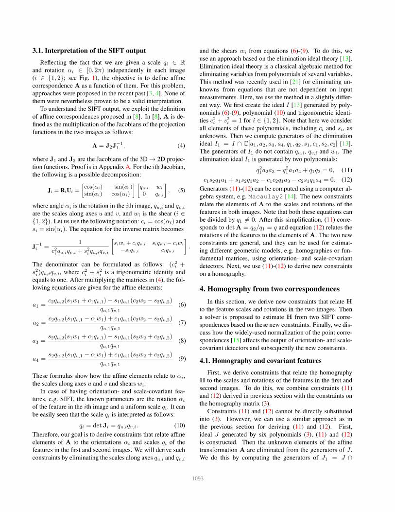
(a) 553 iterations by 2SIFT and
8 615 by 4PT. Inlier ratio 0.38.
(b) 720 iterations by 2SIFT and
78 450 by 4PT. Inlier ratio
0.06.
(c) 169 iterations by 2SIFT and
573 by 4PT. Inlier ratio 0.22.
(d) 65 iterations by 2SIFT and
14 139 by 4PT. Inlier ratio
0.23.
Figure 2: Inliers of the estimated homographies (by 2SIFT) drawn to example image pairs. The numbers of iterations of
GC-RANSAC [7] using the 4PT and proposed 2SIFT solvers; and the ground truth inlier ratios are reported in the captions.
C[h1, . . . , h9, u1, v1, u2, v2, q1, q2, s1, c1, s2, c2]. The elim-
ination ideal J1 is generated by two polynomials:
h8u2s1s2 + h7u2s2c1 − h8v2s1c2 − h7v2c1c2 + (13)
−h2s1s2 − h1s2c1 + h5s1c2 + h4c1c2 = 0,
h27u
21q2 + 2h7h8u1v1q2 + h2
8v21q2 + h5h7u2q1 + (14)
−h4h8u2q1 − h2h7v2q1 + h1h8v2q1 + 2h7h9u1q2 +
2h8h9v1q2 + h2h4q1 − h1h5q1 + h29q2 = 0.
Polynomials (13) and (14) are new constraints that relate
the homography matrix to the scales and rotations of the
features in the first and second images. These constraints
will help us for recovering H from two orientation- and
scale-covariant feature correspondences.
4.2. 2SIFT solver
Constraint (13) is linear in the elements of H. For
two SIFT correspondences, two such equations are given,
which, together with the four equations for point correspon-
dences (2), result in six homogeneous linear equations in
the nine elements of H. In matrix form, these equations
are: Mh = 0, where M is a 6× 9 coefficient matrix and h
contains the unknown homography elements. For two SIFT
correspondences in two views, coefficient matrix M has a
three-dimensional null space. Therefore, the homography
matrix can be parameterized by two unknowns as
H = xH1 + yH2 +H3, (15)
where H1,H2,H3 are created from the 3D null space of
M and x and y are new unknowns. Now we can plug the
parameterization (15) into constraint (14). For two SIFT
correspondences, this results in two quadratic equations in
two unknowns. Such equations have four solutions and they
can be easily solved using e.g. the Grobner basis or the re-
sultant based method [13]. Here, we use the solver based
on Grobner basis method that can be created using the au-
tomatic generator [19]. This solver performs Gauss-Jordan
elimination of a 6× 10 template matrix which contains just
monomial multiples of the two input equations. Then the
solver extracts solutions to x and y from the eigenvectors
of a 4 × 4 multiplication matrix that is extracted from the
template matrix. Finally, up to four real solutions to H are
computed by substituting solutions for x and y to (15).
Note that we do not know any degeneracies of the pro-
posed solver which can occur in real life. For instance, the
degeneracy of the four-point algorithm, i.e. the points are
co-linear, is not a degenerate case for the 2SIFT solver.
4.3. Normalization of the affine parameters
The normalization of the point coordinates is a crucial
step to increase the numerical stability of H estimation [15].
Suppose that we are given a 3× 3 normalizing transforma-
tion Ti transforming the center of gravity of the point cloud
in the ith image to the origin and its average distance from
it to√2. The formula for normalizing A is as follows [6]:
A = T2
[A 00 1
]T−1
1 , (16)
where A is the normalized affinity. Matrix Ti transforms
the points by translating them (last column) and applying
a uniform scaling (diagonal). Due to the fact that the last
column of Ti has no effect on the top-left 2× 2 sub-matrix
of the normalized affinity, the equation can be rewritten as
follows: A = diag(t2, t2) A diag(1/t1, 1/t1) = t2/t1A,
41094
-16 -14 -12 -10 -8 -6 -4 -2
log10
avg. transfer error
0
1
2
3
4
5
Fre
qu
en
cy
104
2SIFT
4PT
3ORB
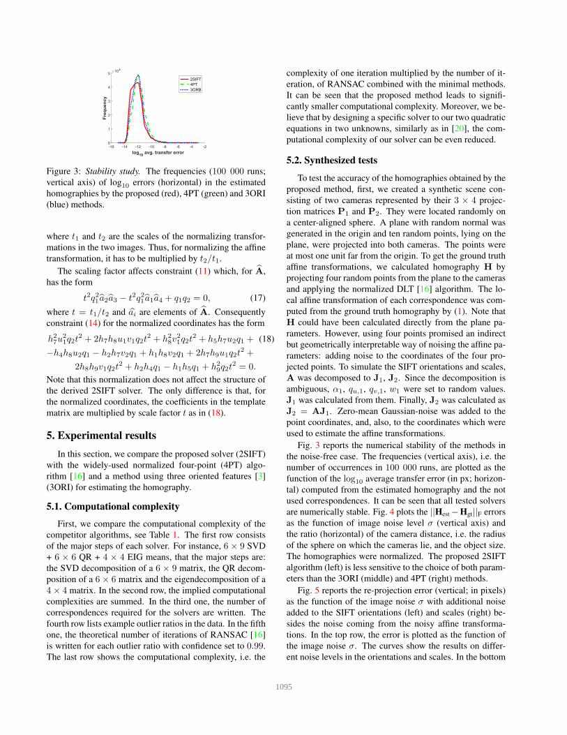
Figure 3: Stability study. The frequencies (100 000 runs;
vertical axis) of log10 errors (horizontal) in the estimated
homographies by the proposed (red), 4PT (green) and 3ORI
(blue) methods.
where t1 and t2 are the scales of the normalizing transfor-
mations in the two images. Thus, for normalizing the affine
transformation, it has to be multiplied by t2/t1.
The scaling factor affects constraint (11) which, for A,
has the form
t2q21 a2a3 − t2q21 a1a4 + q1q2 = 0, (17)
where t = t1/t2 and ai are elements of A. Consequently
constraint (14) for the normalized coordinates has the form
h27u
21q2t
2 + 2h7h8u1v1q2t2 + h2
8v21q2t
2 + h5h7u2q1 + (18)
−h4h8u2q1 − h2h7v2q1 + h1h8v2q1 + 2h7h9u1q2t2 +
2h8h9v1q2t2 + h2h4q1 − h1h5q1 + h2
9q2t2 = 0.
Note that this normalization does not affect the structure of
the derived 2SIFT solver. The only difference is that, for
the normalized coordinates, the coefficients in the template
matrix are multiplied by scale factor t as in (18).
5. Experimental results
In this section, we compare the proposed solver (2SIFT)
with the widely-used normalized four-point (4PT) algo-
rithm [16] and a method using three oriented features [3]
(3ORI) for estimating the homography.
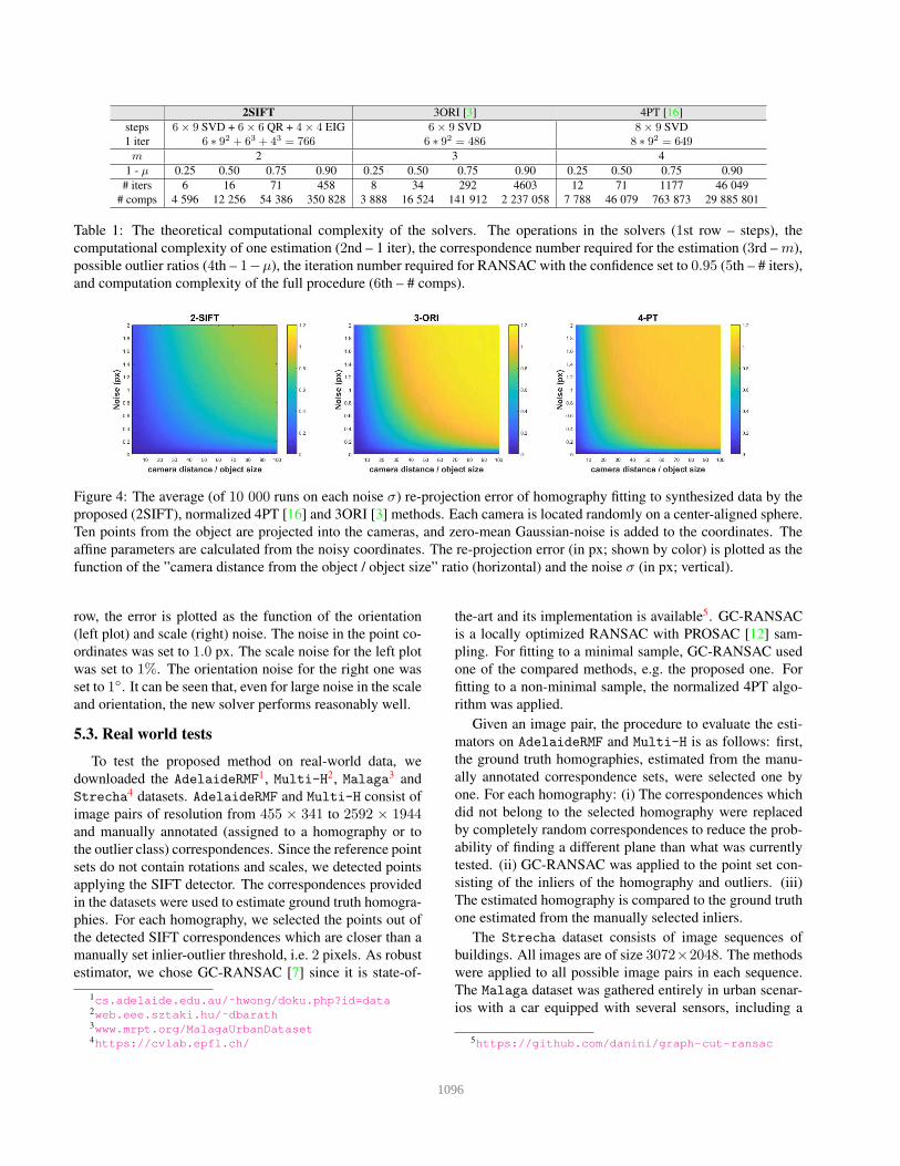
5.1. Computational complexity
First, we compare the computational complexity of the
competitor algorithms, see Table 1. The first row consists
of the major steps of each solver. For instance, 6 × 9 SVD
+ 6 × 6 QR + 4 × 4 EIG means, that the major steps are:
the SVD decomposition of a 6 × 9 matrix, the QR decom-
position of a 6× 6 matrix and the eigendecomposition of a
4× 4 matrix. In the second row, the implied computational
complexities are summed. In the third one, the number of
correspondences required for the solvers are written. The
fourth row lists example outlier ratios in the data. In the fifth
one, the theoretical number of iterations of RANSAC [16]
is written for each outlier ratio with confidence set to 0.99.
The last row shows the computational complexity, i.e. the
complexity of one iteration multiplied by the number of it-
eration, of RANSAC combined with the minimal methods.
It can be seen that the proposed method leads to signifi-
cantly smaller computational complexity. Moreover, we be-
lieve that by designing a specific solver to our two quadratic
equations in two unknowns, similarly as in [20], the com-
putational complexity of our solver can be even reduced.
5.2. Synthesized tests
To test the accuracy of the homographies obtained by the
proposed method, first, we created a synthetic scene con-
sisting of two cameras represented by their 3 × 4 projec-
tion matrices P1 and P2. They were located randomly on
a center-aligned sphere. A plane with random normal was
generated in the origin and ten random points, lying on the
plane, were projected into both cameras. The points were
at most one unit far from the origin. To get the ground truth
affine transformations, we calculated homography H by
projecting four random points from the plane to the cameras
and applying the normalized DLT [16] algorithm. The lo-
cal affine transformation of each correspondence was com-
puted from the ground truth homography by (1). Note that
H could have been calculated directly from the plane pa-
rameters. However, using four points promised an indirect
but geometrically interpretable way of noising the affine pa-
rameters: adding noise to the coordinates of the four pro-
jected points. To simulate the SIFT orientations and scales,
A was decomposed to J1, J2. Since the decomposition is
ambiguous, α1, qu,1, qv,1, w1 were set to random values.
J1 was calculated from them. Finally, J2 was calculated as
J2 = AJ1. Zero-mean Gaussian-noise was added to the
point coordinates, and, also, to the coordinates which were
used to estimate the affine transformations.
Fig. 3 reports the numerical stability of the methods in
the noise-free case. The frequencies (vertical axis), i.e. the
number of occurrences in 100 000 runs, are plotted as the
function of the log10 average transfer error (in px; horizon-
tal) computed from the estimated homography and the not
used correspondences. It can be seen that all tested solvers
are numerically stable. Fig. 4 plots the ||Hest −Hgt||F errors
as the function of image noise level σ (vertical axis) and
the ratio (horizontal) of the camera distance, i.e. the radius
of the sphere on which the cameras lie, and the object size.
The homographies were normalized. The proposed 2SIFT
algorithm (left) is less sensitive to the choice of both param-
eters than the 3ORI (middle) and 4PT (right) methods.
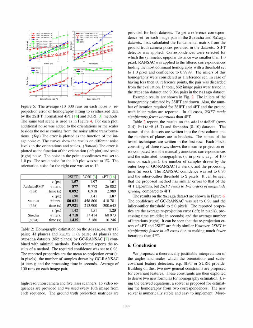
Fig. 5 reports the re-projection error (vertical; in pixels)
as the function of the image noise σ with additional noise
added to the SIFT orientations (left) and scales (right) be-
sides the noise coming from the noisy affine transforma-
tions. In the top row, the error is plotted as the function of
the image noise σ. The curves show the results on differ-
ent noise levels in the orientations and scales. In the bottom
51095
2SIFT 3ORI [3] 4PT [16]
steps 6× 9 SVD + 6× 6 QR + 4× 4 EIG 6× 9 SVD 8× 9 SVD
1 iter 6 ∗ 92 + 63 + 43 = 766 6 ∗ 92 = 486 8 ∗ 92 = 649m 2 3 4
1 - µ 0.25 0.50 0.75 0.90 0.25 0.50 0.75 0.90 0.25 0.50 0.75 0.90
# iters 6 16 71 458 8 34 292 4603 12 71 1177 46 049
# comps 4 596 12 256 54 386 350 828 3 888 16 524 141 912 2 237 058 7 788 46 079 763 873 29 885 801
Table 1: The theoretical computational complexity of the solvers. The operations in the solvers (1st row – steps), the
computational complexity of one estimation (2nd – 1 iter), the correspondence number required for the estimation (3rd – m),
possible outlier ratios (4th – 1−µ), the iteration number required for RANSAC with the confidence set to 0.95 (5th – # iters),
and computation complexity of the full procedure (6th – # comps).
Figure 4: The average (of 10 000 runs on each noise σ) re-projection error of homography fitting to synthesized data by the
proposed (2SIFT), normalized 4PT [16] and 3ORI [3] methods. Each camera is located randomly on a center-aligned sphere.
Ten points from the object are projected into the cameras, and zero-mean Gaussian-noise is added to the coordinates. The
affine parameters are calculated from the noisy coordinates. The re-projection error (in px; shown by color) is plotted as the
function of the ”camera distance from the object / object size” ratio (horizontal) and the noise σ (in px; vertical).
row, the error is plotted as the function of the orientation
(left plot) and scale (right) noise. The noise in the point co-
ordinates was set to 1.0 px. The scale noise for the left plot
was set to 1%. The orientation noise for the right one was
set to 1◦. It can be seen that, even for large noise in the scale
and orientation, the new solver performs reasonably well.
5.3. Real world tests
To test the proposed method on real-world data, we
downloaded the AdelaideRMF1, Multi-H2, Malaga3 and
Strecha4 datasets. AdelaideRMF and Multi-H consist of
image pairs of resolution from 455 × 341 to 2592 × 1944and manually annotated (assigned to a homography or to
the outlier class) correspondences. Since the reference point
sets do not contain rotations and scales, we detected points
applying the SIFT detector. The correspondences provided
in the datasets were used to estimate ground truth homogra-
phies. For each homography, we selected the points out of
the detected SIFT correspondences which are closer than a
manually set inlier-outlier threshold, i.e. 2 pixels. As robust
estimator, we chose GC-RANSAC [7] since it is state-of-
1cs.adelaide.edu.au/˜hwong/doku.php?id=data2web.eee.sztaki.hu/˜dbarath3www.mrpt.org/MalagaUrbanDataset4https://cvlab.epfl.ch/
the-art and its implementation is available5. GC-RANSAC
is a locally optimized RANSAC with PROSAC [12] sam-
pling. For fitting to a minimal sample, GC-RANSAC used
one of the compared methods, e.g. the proposed one. For
fitting to a non-minimal sample, the normalized 4PT algo-
rithm was applied.
Given an image pair, the procedure to evaluate the esti-
mators on AdelaideRMF and Multi-H is as follows: first,
the ground truth homographies, estimated from the manu-
ally annotated correspondence sets, were selected one by
one. For each homography: (i) The correspondences which
did not belong to the selected homography were replaced
by completely random correspondences to reduce the prob-
ability of finding a different plane than what was currently
tested. (ii) GC-RANSAC was applied to the point set con-
sisting of the inliers of the homography and outliers. (iii)
The estimated homography is compared to the ground truth
one estimated from the manually selected inliers.
The Strecha dataset consists of image sequences of
buildings. All images are of size 3072×2048. The methods
were applied to all possible image pairs in each sequence.
The Malaga dataset was gathered entirely in urban scenar-
ios with a car equipped with several sensors, including a
5https://github.com/danini/graph-cut-ransac
61096
0 0.5 1 1.5 2
Noise (px)
0
1
2
3
4
5
6
7
Err
or
(px)
2SIFT, ori. noise = 0.5°
2SIFT, ori. noise = 1.0°
2SIFT, ori. noise = 3.0°
4PT
3ORI, ori. noise = 0.5°
3ORI, ori. noise = 1.0°
3ORI, ori. noise = 3.0°
0 0.5 1 1.5 2
Noise (px)
0
0.5
1
1.5
2
2.5
3
3.5
4
4.5
Err
or
(px)
2SIFT, scale noise = 1%
2SIFT, scale noise = 5%
2SIFT, scale noise = 10%
4PT
3ORI
0 0.5 1 1.5 2 2.5 3
Orientation noise (°)
0
1
2
3
4
5
6
7
8
Err
or
(px
)
2SIFT
4PT
3ORI
0 2 4 6 8 10
Scale noise (%)
1.8
2
2.2
2.4
2.6
2.8
3
3.2
3.4
3.6
Err
or
(px
) 2SIFT
4PT
3ORI
Figure 5: The average (10 000 runs on each noise σ) re-
projection error of homography fitting to synthesized data
by the 2SIFT, normalized 4PT [16] and 3ORI [3] methods.
The same test scene is used as in Figure 4. For each plot,
additional noise was added to the orientations or the scales
besides the noise coming from the noisy affine transforma-
tions. (Top) The error is plotted as the function of the im-
age noise σ. The curves show the results on different noise
levels in the orientations and scales. (Bottom) The error is
plotted as the function of the orientation (left plot) and scale
(right) noise. The noise in the point coordinates was set to
1.0 px. The scale noise for the left plot was set to 1%. The
orientation noise for the right one was set to 1◦.
2SIFT 3ORI [3] 4PT [16]
ǫ (px) 1.57 1.97 1.61
AdelaideRMF # iters. 877 9 772 26 082
(43#) time (s) 0.092 0.918 2.989
ǫ (px) 1.90 3.41 1.87
Multi-H # iters. 80 031 458 800 410 781
(33#) time (s) 57.921 213.900 300.645
ǫ (px) 1.42 1.51 1.25
Strecha # iters. 4 718 17 414 60 973
(852#) time (s) 1.435 3.180 10.246
Table 2: Homography estimation on the AdelaideRMF (18pairs; 43 planes) and Multi-H (4 pairs; 33 planes) and
Strecha datasets (852 planes) by GC-RANSAC [7] com-
bined with minimal methods. Each column reports the re-
sults of a method. The required confidence was set to 0.95.
The reported properties are the mean re-projection error (ǫ,in pixels); the number of samples drawn by GC-RANSAC
(# iters.); and the processing time in seconds. Average of
100 runs on each image pair.
high-resolution camera and five laser scanners. 15 video se-
quences are provided and we used every 10th image from
each sequence. The ground truth projection matrices are
provided for both datasets. To get a reference correspon-
dence set for each image pair in the Strecha and Malaga
datasets, first, calculated the fundamental matrix from the
ground truth camera poses provided in the datasets. SIFT
detector was applied. Correspondences were selected for
which the symmetric epipolar distance was smaller than 1.0pixel. RANSAC was applied to the filtered correspondences
finding the most dominant homography with a threshold set
to 1.0 pixel and confidence to 0.9999. The inliers of this
homography were considered as a reference set. In case of
having less then 50 reference points, the pair was discarded
from the evaluation. In total, 852 image pairs were tested in
the Strecha dataset and 9 064 pairs in the Malaga dataset.
Example results are shown in Fig. 2. The inliers of the
homography estimated by 2SIFT are drawn. Also, the num-
ber of iteration required for 2SIFT and 4PT and the ground
truth inlier ratios are reported. In all cases, 2SIFT made
significantly fewer iterations than 4PT.
Table 2 reports the results on the AdelaideRMF (rows
2–4), Multi-H (5–7) and Strecha (8–10) datasets. The
names of the datasets are written into the first column and
the numbers of planes are in brackets. The names of the
tested techniques are written in the first row. Each block,
consisting of three rows, shows the mean re-projection er-
ror computed from the manually annotated correspondences
and the estimated homographies (ǫ; in pixels; avg. of 100runs on each pair); the number of samples drawn by the
outer loop of GC-RANSAC (# iters.); and the processing
time (in secs). The RANSAC confidence was set to 0.95and the inlier-outlier threshold to 2 pixels. It can be seen
that the proposed method has similar errors to that of the
4PT algorithm, but 2SIFT leads to 1–2 orders of magnitude
speedup compared to 4PT.
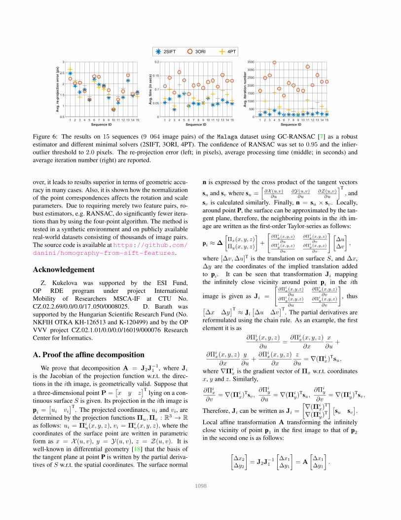
The results on the Malaga dataset are shown in Figure 6.
The confidence of GC-RANSAC was set to 0.95 and the
inlier-outlier threshold to 2.0 pixels. The reported proper-
ties are the average re-projection error (left; in pixels), pro-
cessing time (middle; in seconds) and the average number
of iterations (right). It can be seen that the re-projection er-
rors of 4PT and 2SIFT are fairly similar However, 2SIFT is
significantly faster in all cases due to making much fewer
iterations than 4PT.
6. Conclusion
We proposed a theoretically justifiable interpretation of
the angles and scales which the orientation- and scale-
covariant feature detectors, e.g. SIFT or SURF, provide.
Building on this, two new general constraints are proposed
for covariant features. These constraints are then exploited
to derive two new formulas for homography estimation. Us-
ing the derived equations, a solver is proposed for estimat-
ing the homography from two correspondences. The new
solver is numerically stable and easy to implement. More-
71097
0.72SIFT 3ORI 4PT
1 2 3 4 5 6 7 8 9 10 11 12 13 14 15
Sequence ID
0.5
1
1.5
2
2.5
3
Avg
. re
-pro
jecti
on
err
or
(px)
1 2 3 4 5 6 7 8 9 10 11 12 13 14 15
Sequence ID
0
0.05
0.1
0.15
0.2
Avg
. ti
me (
in s
ecs)
1 2 3 4 5 6 7 8 9 10 11 12 13 14 15
Sequence ID
0
500
1000
1500
2000
2500
3000
3500
Avg
. it
era
tio
n n
um
ber
Figure 6: The results on 15 sequences (9 064 image pairs) of the Malaga dataset using GC-RANSAC [7] as a robust
estimator and different minimal solvers (2SIFT, 3ORI, 4PT). The confidence of RANSAC was set to 0.95 and the inlier-
outlier threshold to 2.0 pixels. The re-projection error (left; in pixels), average processing time (middle; in seconds) and
average iteration number (right) are reported.
over, it leads to results superior in terms of geometric accu-
racy in many cases. Also, it is shown how the normalization
of the point correspondences affects the rotation and scale
parameters. Due to requiring merely two feature pairs, ro-
bust estimators, e.g. RANSAC, do significantly fewer itera-
tions than by using the four-point algorithm. The method is
tested in a synthetic environment and on publicly available
real-world datasets consisting of thousands of image pairs.
The source code is available at https://github.com/
danini/homography-from-sift-features.
Acknowledgement
Z. Kukelova was supported by the ESI Fund,
OP RDE program under project International
Mobility of Researchers MSCA-IF at CTU No.
CZ.02.2.69/0.0/0.0/17 050/0008025. D. Barath was
supported by the Hungarian Scientific Research Fund (No.
NKFIH OTKA KH-126513 and K-120499) and by the OP
VVV project CZ.02.1.01/0.0/0.0/16019/000076 Research
Center for Informatics.
A. Proof the affine decomposition
We prove that decomposition A = J2J−11 , where Ji
is the Jacobian of the projection function w.r.t. the direc-
tions in the ith image, is geometrically valid. Suppose that
a three-dimensional point P =[x y z
]Tlying on a con-
tinuous surface S is given. Its projection in the ith image is
pi =[ui vi
]T. The projected coordinates, ui and vi, are
determined by the projection functions Πu,Πv : R3 → R
as follows: ui = Πiu(x, y, z), vi = Πi
v(x, y, z), where the
coordinates of the surface point are written in parametric
form as x = X (u, v), y = Y(u, v), z = Z(u, v). It is
well-known in differential geometry [18] that the basis of
the tangent plane at point P is written by the partial deriva-
tives of S w.r.t. the spatial coordinates. The surface normal
n is expressed by the cross product of the tangent vectors
su and sv where su =[∂X (u,v)
∂u
∂Y(u,v)∂u
∂Z(u,v)∂u
]T
, and
sv is calculated similarly. Finally, n = su × sv . Locally,
around point P, the surface can be approximated by the tan-
gent plane, therefore, the neighboring points in the ith im-
age are written as the first-order Taylor-series as follows:
pi ≈ ∆
[Πx(x, y, z)Πy(x, y, z)
]+
[∂Πi
x(x,y,z)
∂u
∂Πix(x,y,z)
∂v∂Πi
y(x,y,z)
∂u
∂Πiy(x,y,z)
∂v
] [∆u
∆v
],
where [∆v,∆u]T is the translation on surface S, and ∆x,
∆y are the coordinates of the implied translation added
to pi. It can be seen that transformation Ji mapping
the infinitely close vicinity around point pi in the ith
image is given as Ji =
[∂Πi
x(x,y,z)∂u
∂Πix(x,y,z)∂v
∂Πiy(x,y,z)
∂u
∂Πiy(x,y,z)
∂v
], thus
[∆x ∆y
]T ≈ Ji[∆u ∆v
]T. The partial derivatives are
reformulated using the chain rule. As an example, the first
element it is as
∂Πix(x, y, z)
∂u=
∂Πix(x, y, z)
∂x
x
∂u+
∂Πix(x, y, z)
∂x
y
∂u+
∂Πix(x, y, z)
∂x
z
∂u= ∇(Πi
x)Tsu,
where ∇Πix is the gradient vector of Πx w.r.t. coordinates
x, y and z. Similarly,
∂Πix
∂v= ∇(Πi
x)T
sv,∂Πi
y
∂u= ∇(Πi
y)T
su,∂Πi
y
∂v= ∇(Πi
y)T
sv,
Therefore, Ji can be written as Ji =
[∇(Πi
x)T
∇(Πiy)
T
] [su sv
].
Local affine transformation A transforming the infinitely
close vicinity of point p1 in the first image to that of p2
in the second one is as follows:
[∆x2
∆y2
]= J2J
−11
[∆x1
∆y1
]= A
[∆x1
∆y1
].
81098
References
[1] Daniel Barath. P-HAF: Homography estimation using par-
tial local affine frames. In International Conference on Com-
puter Vision Theory and Applications, 2017. 2
[2] Daniel Barath. Approximate epipolar geometry from six ro-
tation invariant correspondences. In International Confer-
ence on Computer Vision Theory and Applications, 2018. 2
[3] Daniel Barath. Five-point fundamental matrix estimation for
uncalibrated cameras. In Conference on Computer Vision
and Pattern Recognition, 2018. 2, 3, 5, 6, 7
[4] Daniel Barath. Recovering affine features from orientation-
and scale-invariant ones. In Asian Conference on Computer
Vision, 2018. 2, 3
[5] Daniel Barath and Levente Hajder. A theory of point-wise
homography estimation. Pattern Recognition Letters, 94:7–
14, 2017. 1
[6] Daniel Barath and Levente Hajder. Efficient recovery of es-
sential matrix from two affine correspondences. IEEE Trans-
actions on Image Processing, 27(11):5328–5337, 2018. 1, 4
[7] Daniel Barath and Jiri Matas. Graph-Cut RANSAC. In Con-
ference on Computer Vision and Pattern Recognition, 2018.
2, 4, 6, 7, 8
[8] Daniel Barath, J. Molnar, and Levente Hajder. Optimal sur-
face normal from affine transformation. In International
Joint Conference on Computer Vision, Imaging and Com-
puter Graphics Theory and Applications. SciTePress, 2015.
1, 3
[9] Daniel Barath, T. Toth, and Levente Hajder. A minimal so-
lution for two-view focal-length estimation using two affine
correspondences. In Conference on Computer Vision and
Pattern Recognition, 2017. 1
[10] Herbert Bay, Tinne Tuytelaars, and Luc Van Gool. SURF:
Speeded up robust features. European Conference on Com-
puter Vision, 2006. 1, 2
[11] Jacob Bentolila and Joseph M. Francos. Conic epipolar con-
straints from affine correspondences. Computer Vision and
Image Understanding, 2014. 1
[12] Ondrej Chum and Jiri Matas. Matching with PROSAC-
progressive sample consensus. In Computer Vision and Pat-
tern Recognition, 2005. 6
[13] David Cox, John Little, and Donal O’Shea. Using Algebraic
Geometry. Springer-Verlag New York, 2nd edition, 2005. 3,
4
[14] Daniel Grayson and Michael Stillman. Macaulay2, a soft-
ware system for research in algebraic geometry. available at
www.math.uiuc.edu/Macaulay2/. 3
[15] Richard Hartley. In defense of the eight-point algorithm. Pat-
tern Analysis and Machine Intelligence, 1997. 3, 4
[16] Richard Hartley and Andrew Zisserman. Multiple view ge-
ometry in computer vision. Cambridge University Press,
2003. 2, 5, 6, 7
[17] Kevin Koser. Geometric Estimation with Local Affine
Frames and Free-form Surfaces. Shaker, 2009. 1
[18] Erwin Kreyszig. Introduction to differential geometry and
Riemannian geometry, volume 16. University of Toronto
Press, 1968. 8
[19] Zuzana Kukelova, Martin Bujnak, and Tomas Pajdla. Auto-
matic generator of minimal problem solvers. In European
Conference on Computer Vision, volume 5304 of Lecture
Notes in Computer Science, 2008. 4
[20] Zuzana Kukelova, Jan Heller, and Andrew Fitzgibbon. Effi-
cient intersection of three quadrics and applications in com-
puter vision. In Conference on Computer Vision and Pattern
Recognition, pages 1799–1808, 2016. 5
[21] Zuzana Kukelova, Joe Kileel, Bernd Sturmfels, and Tomas
Pajdla. A clever elimination strategy for efficient minimal
solvers. In Conference on Computer Vision and Pattern
Recognition, 2017. http://arxiv.org/abs/1703.05289. 3
[22] David G. Lowe. Object recognition from local scale-
invariant features. In International Conference on Computer
vision, 1999. 1, 2
[23] Jiri Matas, Ondrej Chum, Martin Urban, and Tomas Pajdla.
Robust wide-baseline stereo from maximally stable extremal
regions. Image and vision computing, 2004. 2
[24] Kristian Mikolajczyk, Tinne Tuytelaars, Cordelia Schmid,
Andrew Zisserman, Jiri Matas, Frederik Schaffalitzky, Timor
Kadir, and Luc Van Gool. A comparison of affine region
detectors. International Journal of Computer Vision, 65(1-
2):43–72, 2005. 1
[25] Steven Mills. Four-and seven-point relative camera pose
from oriented features. In International Conference on 3D
Vision, pages 218–227. IEEE, 2018. 2
[26] Dmytro Mishkin, Jiri Matas, and Michal Perdoch. MODS:
Fast and robust method for two-view matching. Computer
Vision and Image Understanding, 2015. 1, 2
[27] J. Molnar and D. Chetverikov. Quadratic transformation for
planar mapping of implicit surfaces. Journal of Mathemati-
cal Imaging and Vision, 2014. 2
[28] Jean-Michel Morel and Guoshen Yu. ASIFT: A new frame-
work for fully affine invariant image comparison. SIAM jour-
nal on imaging sciences, 2(2):438–469, 2009. 1
[29] Michal Perdoch, Jiri Matas, and Ondrej Chum. Epipolar ge-
ometry from two correspondences. In International Confer-
ence on Pattern Recognition, 2006. 1
[30] James Pritts, Zuzana Kukelova, Viktor Larsson, and Ondrej
Chum. Radially-distorted conjugate translations. Conference
on Computer Vision and Pattern Recognition, 2018. 1
[31] Carolina Raposo and Joao P. Barreto. πmatch: Monocular
vslam and piecewise planar reconstruction using fast plane
correspondences. In European Conference on Computer Vi-
sion, pages 380–395. Springer, 2016. 1
[32] Carolina Raposo and Joao P. Barreto. Theory and practice
of structure-from-motion using affine correspondences. In
Computer Vision and Pattern Recognition, 2016. 1
[33] Ethan Rublee, Vincent Rabaud, Kurt Konolige, and Gary
Bradski. ORB: An efficient alternative to sift or surf. In
International Conference on Computer Vision, pages 2564–
2571. IEEE, 2011. 2
91099


![[Mark Burgess] Classical Covariant Fields(BookFi.org)](https://img.pdfslide.us/doc/110x75/55cf97d8550346d03393f46c/mark-burgess-classical-covariant-fieldsbookfiorg.jpg)