JOURNAL OF Econometrics Efficient estimation and ... · Econometrics Efficient estimation and stratified sampling ... The complications arise if we have both ... We are interested

ELSEVIER Journal of Econometrics 74 (1996) 289-318

JOURNAL OF Econometrics

Efficient estimation and stratified sampling

G u i d o W. I m b e n s *'~ , T o n y L a n c a s t e r b

a Department of Economics, Harvard University, Cambridge, MA 02138, USA b Department of Economics. Brown University. Providence, RI 02912, USA

(Received June 1992; final version received March 1995)

Abstract

In this paper we investigate estimation of a class of semi-parametric models. The part of the model that is not specified is the marginal distribution of the explanatory variables. The sampling is stratified on the dependent variables, implying that the explanatory variables are no longer exogenous or ancillary. We develop a new estimator for this estimation problem and show that it achieves the semi-parametric efficiency bound for this case. In addition we show that the estimator applies to a number of sampling schemes that have previously been treated separately.

Key words: Stratified sampling; Endogenous sampling JEL classification: C33; C35; (241; C42

1. Introduction

In econometric analyses one often assumes that observations are drawn randomly from a large population. In reality it might neither be true, nor need it be desirable to have such a sample. In this paper we will investigate how inference might proceed for a particular class o f nonrandom sampling schemes.

The starting point is a model in which two types o f variables are distin- guished. The first arc the dependent variables whose distribution is to be ex- plained in terms o f the variables o f the second type. The latter will be referred to as explanatory, independent, or regressor variables. We will assume that the researcher has specified a parametric family for the distribution o f the

* Corresponding author. We would like to thank a referee, an associate editor, Joshua Angfist, Ricardo Barros, Gary Chamberlain, Geert Ridder, and participants in seminars at Northwestern University, the University of Chicago, the Harvard/MIT econometrics seminar, and the Brown/Yale workshop for comments, and the NSF for support under grant SES 9122477.

0304-4076/96/$15.00 © 1996 Elsevier Science S.A. All rights reserved SSD! 0 3 0 4 - 4 0 7 6 ( 9 5 ) 0 1 7 5 6 - 4

290 G.W. lmbens, 1". Lancaster~Journal of Econometrics 74 (1996) 289-318

dependent variable conditional on the explanatory variables. Interest centers on the parameters of this conditional distribution. We do not make assumptions about the marginal distribution of the regressors other than assuming that they do not depend on the parameters of the aforementioned conditional distribution.

If the sampling were random, the parameters of the conditional distribution could be estimated consistently and efficiently by maximizing the conditional likelihood function. Even if the sampling were exogenous, by which we mean that the probability of a unit of the population being sampled depends on the values of the explanatory variables, this method would lead to consistent and efficient estimates. We investigate sampling strategies that imply that the probability of being sampled depends directly on the value of the dependent or endogenous variables. The particular sampling schemes that we consider are based on a stratification of the sample space. The sampling is not random because the probability that a unit is drawn from a particular stratum is not equal to the probability that an unit randomly drawn from the whole population is from that stratum. Within the strata however, the sampling and population distribution are identical. This is referred to in the literature as stratified sampling (Jewell, 1985), endogenous sampling (Hausman and Wise, 1981 )~ or biased sampling (Gill, Vardi, and Wellner, 1988).

Another way of looking at this is in terms of the aneillarity or exogeneity of the explanatory variables. If the sample is random or exogenous, the marginal distribution of the regressors does not depend on the parameters of interest. When the sampling is endogenous, the marginal distribution of the regressors in th-, sample does depend on the parameters of interest, and consequently the regressors are no longer ancillary or exogenous. The guiding principle is that one should not condition the analysis on variables that are not ancillary, because that might lead to a loss of efficiency, and one should condition on variables that are ancillary, because a failure to do so can lead to paradoxical results.

As an example, consider the following standard linear model:

Y = X ' ~ + ~ , e IX ~ ~r(O, a2). (I)

If the density of X is h(x), for x E ~ , the joint density of Y and X can be written a s

f ( y , x ) = -~ , - - - ~ - - - / • h(x),

where 4~(') is the standard normal density function. Suppose that instead of a random sample generated according to the model in (1), we have Ni observations drawn randomly from the truncated sample space ( -oo,0] × ~ and Are observations drawn randomly from the truncated sample space (0 ,oo)x ~ . The

G. W. Imbens, T. £ ~ncaster I Journal of Econometrics 74 (1996) 289-318 291

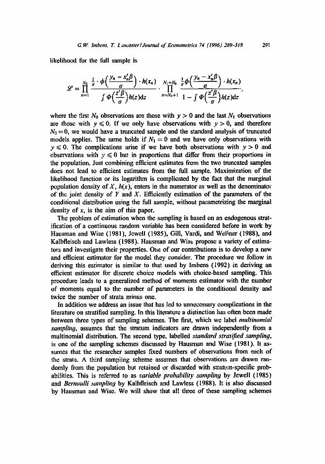
likelihood for the full sample is

, .h(x.) No~ ~ = l-I ~ J

J"'3 I1 ~ / z' fl

where the first No observations arc those with y > 0 and the last N1 observations are those with y ~< 0. If we only have observations with y > 0, and therefore No = 0, we would have a truncated sample and the standard analysis of truncated models applies. The same holds if Nn = 0 and we have only observations with y ~ 0. The complications arise if we have both observations with y > 0 and observations with y ~ 0 but in proportions that differ from their proportions in the population. Just combining efficient estimates from the two truncated samples does not lead to efficient estimates from the full sample. Maximization of the likelihood function or its logarithm is complicated by the fact that the marginal population density of X, h(x), enters in the numerator as well as the denominator of the joint density of Y and X. Efficiently estimation of the parameters of the conditional distribution using the full sample, without parametrizing the marginal density of x, is the aim of this paper.

The problem of estimation when the sampling is based on an endogenous stratification of a continuous random variable has been considered before in work by Hausman and Wise (1981), Jewell (1985), Gill, Vardi, and Weilner (1988), and Kalbfleisch and Lawless (1988). Hausman and Wis~ propose a variety of estimators and investigate their properties. One of our contributions is to develop a new and efficient estimator for the model they consider. The procedure we follow in deriving this estimator is similar to that used by lmbens (1992) in deriving an efficient estimator for discrete choice models with choice-based sampling. This procedure leads to a generalized method of moments estimator with the number of moments equal to the number of parameters in the conditional density and twice the number of strata minus one.

In addition we address an issue that has led to unnecessary complications in the literature on stratified sampling. In this literature a distinction has often been made between three types of sampling sehemes. The first, which we label multinomial sampling, assumes that the stratum indicators are drawn independently from a multinomiai distribution. The second type, labelled standard stratified sampling, is one of the sampling schemes discussed by Hausman and Wise (1981). It assumes that the researcher samples fixed numbers of observations from each of the strata. A third sampling scheme assumes that observations are drawn randomly from the population but retained or discarded with stratl,,m-specific probabilities. This is referred to as variable probability samplinff by Jewell (1985) and Bernoulli samplinff by Kalbfleisch and Lawless (1988). It is also discussed by Hausman and Wise. We will show that all three of these sampling schemes

292 G.W. Imbens, T. Lancaster~Journal of Econometrics 74 (1996) 289--318

allow the researcher to use the estimation procedure that will be developed in this paper.

The plan of the paper is as follows: In the next section the three sampling schemes will be discussed. It will be argued that they are all in principle amenable to the same estimation procedures. Section 3 contains the efficient estimation procedure. It will be derived in two steps. First we analyze the case where the regressors have a discrete distribution. Then we rewrite the equations characterizing the maximum likelihood estimates in such a way that they do no longer require discreteness of the explanatory variables. In Section 4 we analyze two examples with the normal linear model and discus,~ the relations to the analysis of truncated models. In the last section some concluding remarks will be made and the main findings of the paper will be summarized.

2. Sampling schemes and likelihood functions

The notation in analyses where the sampling is nonrandom is usually cumbersome. To some extent this cannot be avoided. One has to distinguish between the population distribution on the one hand and the distribution according to which the data are distributed on the other hand. If the sampling is random, these two are equal, and if the sampling is exogenous, they differ but in a way immaterial for the purposes of inference about the parameters of the conditional distribution. Only in the case where the sampling is dependent on the endogenous variable is the difference important. In this paper we try to keep the notation transpar- ent without making it imprecise. Most of the notation will be introduced in the first subsection. There we introduce the sampling scheme that we will work with through most of the paper. In the second subsection we discuss standard stratified sampling. In the third subsection Bernoulli sampling or variable probability sampling will be discussed.

2.1. Multinomial sampli~g

Let Y and X be two, possibly vector-valued, random variables defined on x ~ . The joint probability density function in the population is

f ( y , x ) = f ( y Ix,//). h(x), (2)

where fO ' Ix,//) is a known function of y, x and an unknown parameter//, and h(x) is an unknown function. We are interested in the parameter//of the conditional distribution of Y given X. We are not willing to make assumptions about the marginal distribution of X. In that sense the problem is a semi-parametric

G. W. Imbens, T. Lancaster l Journal of Econometrics 74 (1996) 289-318 293

one. With respect to fl, X is exogenous or ancillary ~ and Y is endogenous. I f one had at one's disposal a random sample of X and Y, one could estimate fl by maximizing the logarithm of the conditional likelihood function:

N L(fl) = ~ In f(Yn Ixn, fl ). ~3)

n=l

Because the marginal distribution of X does not depend on fl, conditioning on x does not entail a loss of efficiency, and there is no need to specify h(x) more fully.

However, if the sampling scheme is not random, this easy separation no longer exists in general. If the sampling is exogenous, i.e., the probability of being sampled depends only on the exogenous variable X, then maximization of (3) s';ili leads to a consistent estimator for/~. We are, however, interested in more general sampling schemes where the probability of being sampled depends on Y as well as X. This makes the reluctance to specify h(x) a more complicated issue.

Let ~s, for s = 1 . . . . T, be subsets of ~ x ~r. The ~s are the strata from which the observations are to be drawn. The probability of a randomly drawn observation lying in ~s is

Qs = f% f ( y Ix, fl)h(x)dydx. (4)

The basic sampling scheme that we will in the course of this paper refer to as multinomial sampling, is as follows: with probability Hs we draw an observation randomly from r,gs. The Hs are the sampling probabilities with Hr shorthand for ! - Y~'~sr..~ I H~. With discrete Y this is the sampling scheme discussed by Manski and McFadden (1981) in their analysis of choice-based sampling.

Examples of sampling strategies that fit in this framework are:

1. T = 1, g~ = ~,~ x k r. Random sampling.

2. r#~ = c#/ x .~r, where . ~ C k r. Pure exogenous sampling. Maximization of the random sampling conditional likelihood still gives consistent and efficient estimates.

3. ~ = ~/~ x ~" where .~/~ C ~ . Pure endogenous sampling.

4. ~ = o~ x .~r, ~2 C o?/x gt'. In this case we have a random sample augmented with extra observations drawn from part of the sample space.

r oj,. 5. cgsN~t = {~ if s ~ t, and Us=l~S = ~ x This will be labelled a partioned sample. In this case the population probabilities Q~ add up to one. This is not necessarily the case for other sampling schemes.

I See Cox and Hinkley (1974) for a discussion of ancillarity and Engle et al. (1982) for a discussion of the related concept of exogeneity.

294 G.W. Imbens, T. Lancaster~Journal of Econometrics 74 (1996) 289-318

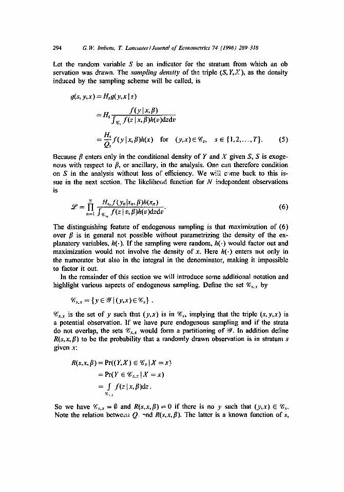
Let the random variable S be an indicator for the stratum from which an ob servation was drawn. The sampling density of the triple (S, Y,X), as the density induced by the sampling scheme will be called, is

9(s, y ,x ) = Hsg(y,x Is)

f (y lx , fl) = Hs f % f ( z Ix, fl)h(v)dzdv

Hs =-~sf(y[x, fl)h(x ) for (y,x)e~,s, s e { l , 2 . . . . . T}. (5)

Because/? enters only in the conditional density of Y and X given S, S is exogenous with respect to fl, or ancillary, in the analysis. One. call therefore condition on S in the analysis without loss o~" efficiency. We will c~me back to this issue in the next section. The likelihood function for N independent observations is

~" Hs,,f(ynlX,, fl)h(xn) ~o = I-[ (6)

n=l f % f ( z l v,[:l)h(v)dzdv"

The distinguishing feature of endogenous sampling is that maximization of (6) over fl is in general not possible without parametrizing the density of the explanatory variables, h(-). If the sampling were random, h(.) would factor out and maximization would not involve the density of x. Here h(-) enters not only in the numerator but also in the integral in the denominator, making it impossible to factor it out.

In the remainder of this section we will introduce some additional notation and highlight various aspects of endogenous sampling. Define the set ~,..x by

~es.x= {yc?¢l(y,x)e~'~} .

~gs.x is the set of y such that (y,x) is in ~s, implying that the triple (s ,y ,x) is a potential observation. If we have pure endogenous sampling and if the strata do not overlap, the sets ~gs, x would form a partitioning of ~ . In addition define R(s,x, fl) to be the probability that a randomly drawn observation is in stratum s given x:

g(s,x, [I) = a r ( ( r , x ) S ~6.~ IX = x)

= Pr(Y E Y~.x IX = x )

= f f ( z Ix,/J)dz.

So we have ~6(,.,x = 0 and R(s.,x, f l )= 0 if there is no y such that (y,x) E c8,.. Note the relation betweeLt Q. ",nd R(s,x, li). The latter is a known function of s,

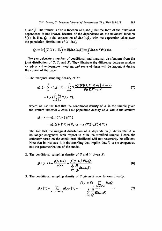
G.W. Imbens. T. Lancasterl Journal of Econometrics 74 (1996) 289-318 295

x, and ft. The former is also a function of s and fl but the form of the functional dependence is not known, because of the dependence on the unknown function h(x). In fact, Q~ is the expectation of R(s,X, fl), with the expecation taken over the population distribution of X, h(x),

Qs = Pr((Y,X) E ,~,) = E[R(s,X, fl)] = fR( s , x , fl)P,(x),~, x

We can calculate a number of conditional and marginal distributions from the joint distribution of S, Y, and X. They illustrate the difference between random sampling and endogenous sampling and some of them will be important during the course of the paper.

1. The marginal sampling density of X:

r ~r H, h(x)P((r ,x) ~ ~,, I X = x) O(x) = ~, Hto(xl t ) = (7)

t=, t=, P( (Y ,X) E c(,t

r n t = h(x) Y~ -~-R(t,x, fl),

t= l ~dt

where we use the fact that the con~'itional density of X in the sample given the stratum indicator S equals the population density of X within the stratum:

o(x Is) = h(x I ( v , x ) ~ 'e,~)

= h(x)P((Y,X) E ~,,'t iX = x) /P( (Y ,X) E ~,t).

The fact that the marginal distribution of X depends on fl shows that X is no longer exogenous with respect to // in the stratified sample. Hence the estimator based on the conditional likelihood will not necessarily be efficient. Note that in this case it is the sampling that implies that X is not exogenous, not the parametrization of the model.

2. The conditional sampling density of S and Y given X:

O(s, y Ix) = o(s, y,x) _ f ( y Ix, ~)H, IQ, (8) O(x ) f~ Ht

t= l Qt R(t'X' ~)

3. The conditional sampling density of Y given X now follows directly:

f ( y I x, fl) Y] Ht/Qt 9 ( y l x ) = ~ O(y , t [ x )= t IO',x)e% (9)

r H , t I (y.s)~% t=l~ -Qt R(t'x' fl)

296 G. IV. Imbens, T, Lancaster~Journal of Econometrics 74 (1996) 289-318

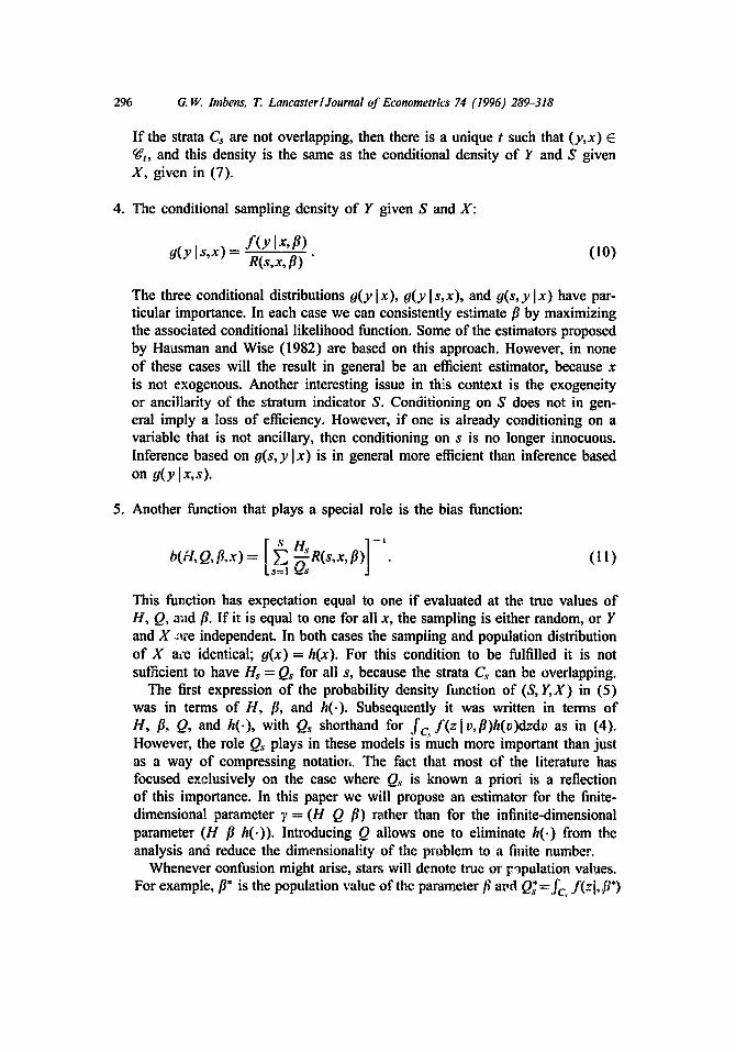
If the strata C~ are not overlapping, then there is a unique t such that (y,x) E ~'t, and this density is the same as the conditional density of Y and S given X, given in (7).

4. The conditional sampling density of Y given S and X:

f ( y l x , fl) O(Y Is, x) = R(s,x, fl) " (10)

The three conditional distributions g(y Ix), g(yls, x), and O(s, y lx) have par- titular importance. In each ease we can consistently estimate fl by maximizing the associated conditional likelihood function. Some of the estimators proposed by Hausman and Wise (1982) are based on this approach. However, in none of these eases will the result in general be an efficient estimator, because x is not exogenous. Another interesting issue in this context is the exogeneity or anci!larity of the stratum indicator S. Conditioning on S does not in general imply a loss of efficiency. However, if one is already conditioning on a variable that is not ancillary, then conditioning on s is no longer innocuous. Inference based on g(s,y Ix) is in general more efficient than inference based on g(y Ix, s).

5. Another function that plays a special role is the bias function:

b(,~, Q, p,x) = R(s,x,[O (11) s = !

This function has expectation equal to one if evaluated at the true values of H, Q, aad ft. If it is equal to one for all x, the sampling is either random, or Y and X ,are independent. In both cases the sampiing and population distribution of X ace identical; g(x)= h(x). For this condition to be fulfilled it is not sufficient to have Hs = Qs for all s, because the strata Cs can be overlapping.

The first expression of the probability density function of (S, Y,X) in (5) was in terms of H, fl, and h(.). Subsequently it was written in terms of H, fl, Q, and h(.), with Q~ shorthand for f c f ( z l v , fl)h(v)dzdv as in (4). However, the role Qs plays in these models is much more important than just as a way of compressing notation,. The fact that most o f the literature has focused exclusively on the case where Qs is known a priori is a reflection of this importance. In this paper we will propose an estimator for the finite- dimensional parameter ~, = (H Q fl) rather than for the infinite-dimensional parameter (H fl h(.)). Introducing Q allows one to eliminate h(.) from the analysis and reduce the dimensionality of the problem to a finite number.

Whenever confusion might arise, stars will denote true or F~pulation values. * " Z * For example, fl* is the population value of thc parameter fi ai,d Q~ =Jc~ f ( l, [J )

G.W. Imbens, T. Lancasterl Journal of Econometrics 74 (1996) 289-318 297

h(v)dzdv is the true population proportion of people in stravam s. The estimator that will be derived will allow for incorporation of linear restrictions on H, Q, and fl (with the restriction Q = Q* the most important of these) in a straightforward manner.

2.2. Standard stratified sampling

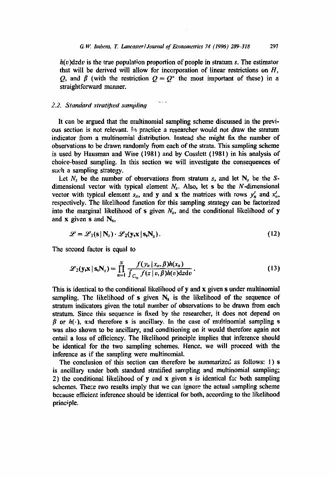
It can be argued that the multinomial sampling scheme discussed in the previous section is not relevant, gn practice a researcher would not draw the stratum indicator from a multinomial distribution. Instead she might fix the number of observations to be drawn randomly from each of the strata. This sampling scheme is used by Hausman and Wise (1981) and by Cosslett (1981) in his analysis of choice-based sampling. In this section we will investigate the consequences of such a sampling strategy.

Let Ns be the number of observations from stratum s, and let N~ be the S- dimensional vector with typical element N~. Also, let s be the N-dimensional vector with typical element s,,, and y and x the matrices with rows y" and x', respectively. The likelihood function for this sampling strategy can be factorized into the marginal likelihood of s given N~, and the conditional likelihood of y and x given s and Ns,

= ~ ' l (s I Ns) • Ae2(y,x I s,Ss). (12)

The second factor is equal to

N f (Yn ]xn, fl)h(xn) ~e2(y,x I s,Ns) = 1-[

,,=l f ¢~, f ( z I v, fl)h(v)dzdv " (13)

This is identical to the conditional likelihood of y and x given s under multinomial sampling. The likelihood of s given Ns is the likelihood of the sequence of stratum indicators given the total number of observations to be drawn from each stratum. Since this sequence is fixed by the researcher, it does not depend on fl or h(.), and therefore s is ancillary. In the ease of multinomia! sampling s was also shown to be ancillary, and conditioning on it would therefore again not entail a loss of efficiency. The likelihood principle implies that inference should be identical for the two sampling schemes. Hence, we will proceed with the inference as if the sampling were multinomial.

The conclusion of this section can therefore be summarized as follows: !) s is ancillary under both standard stratified sampling and multinomial sampling; 2) the conditional likelihood of y and x given s is identical foz ~ both sampling schemes. The~e two results imply that we can ignore the actual sampling scheme because efficient inference should be identical for both, according to the likelihood principle.

298 G.W. Imbens, T. Lancasterl Jo~rnal of Econometrics 74 (1996) 289-318

2.3. Bernoulli samplirg

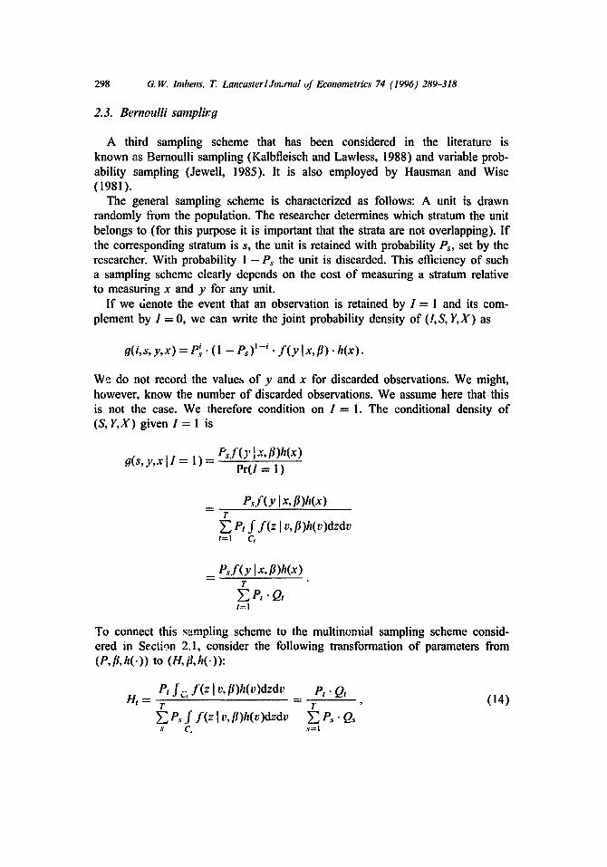
A third sampling scheme that has been considered in the literature is known as Bernoulli sampling (Kalbfleisch and Lawless, 1988) and variable probability sampling (Jewell, 1985). It is also employed by Hausman and Wise (1981).

The general sampling scheme is characterized as follows: A unit is drawn randomly from the population. The researcher determines which stratum the unit belongs to (for this purpose it is important that the strata are not overlapping). If the corresponding stratum is s, the unit is retained with probability Ps, set by the researcher. With probability 1 - P s the unit is discarded. This efficiency of such a sampling scheme clearly depends on the cost of measuring a stratum relative to measuring x and y for any unit.

If we denote the event that an observation is retained by I = l and its com- plement by I = 0, we can write the joint probability density of (1,S, Y,X) as

_ i 9(i,s,y,x) -- P's" (1 - Ps) I-i . f ( y Ix, fl). h(x).

We do not record the values of y and x for discarded observations. We might, however, know the number of discarded observations. We assume here that this is not the ease. We therefore condition on I = 1. The conditional density of (S, Y,X) given 1 = 1 is

e(s,y, xl l = ! ) = PsfO' Ix, fl)h(x)

Pr(J = 1 )

Psf(Y Ix, fl)h(x) T

Pt f f ( z I v, ll)h(v)dzdv 1=1 Ct

= P~f(y Ix, fl)h(x) T

EP, .Q, t= l

To connect this sampling scheme to the multinomiai sampling scheme considered in Section 2.1, consider the following transformation of parameters from (P, fl, h(.)) to (n,/3,h(-)):

P, fc, f(z Iv, B)h(v)d dv P," Qt H t = T T

~P~ f f(z]v, fl)h(v)dzdv ~_,P,,.Q,~ s C~ s= I

(14)

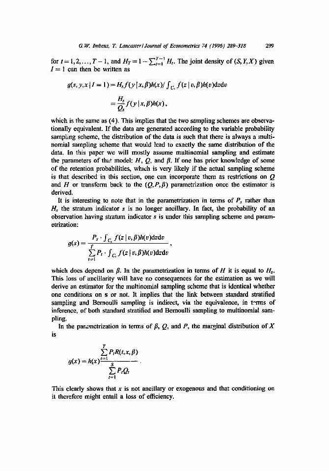
G.W. Imbens, 1". Lancasterl Journal of Econometrics 74 (1996) 289-318 299

T--I for t= 1,2 . . . . . T - 1, and Hr = 1 -~"~t=l Hr. The joint density of (S, Y,X) given I = 1 can then be written as

O(s, y ,x II = 1 ) = H s f ( y Ix, fl)h(x)/ f c , f ( z I v, fl)h(v)dzdv

= ~ s f ( y lx, fl)h(x),

which is the same as (4). This implies that the two sampling schemes are observa- tionally equivalent. If the data are generated according to the variable probability sampling scheme, the distribution of the data is such that there is always a multinomial sampling scheme that would lead to exactly the same distribution of the data. In fills paper we will mostly assume multinomial sampling and estimate the parameters of that model: H, Q, and ~. If one has prior knowledge of some of the retention probabilities, which is very likely if the actual sampling scheme is that described in this section, one can incorporate them as restrictions on Q and H or transform back to the (Q,P,~) parametrization once the estimator is derived.

It is interesting to note that in the parametrization in terms of Ps rather than Hs the stratum indicator s is no longer ancillary. In fact, the probability of an observation having stratum indicator s is under this sampling scheme and parametrization:

Ps " f c, f(zlv'fl)h(v)dzdv o ( s ) = r

P" f c, f ( z [ v,~)h(v)dzdv t=l

which does depend on ft. In the parametrization in terms of H it is equal to Hs. This loss of ancillarity will have no consequences for the estimation as we will derive an estimator for the multinomial sampling scheme that is identical whether one conditions on s or not. It implies that the lirak between standard stratified sampling and Bernoulli sampling is indirect, via the equivalence, in t~rms of inference, of both standard stratified and Bernoulli sampling to multinomial sampling.

In the parametrization in terms of fl, Q, and P, the marginal distribution of X is

T

Y] PtR( t,x, fl) o(x) = h ( x ) '=~ s

E P, Q, t=l

This clearly shows that x is not ancillary or exogenous and that conditioning on it therefore might entail a loss of efficiency.

300 G.W. lmbens, T. Lancaster/Journal of Econometrics 74 (1996) 289-318

We have shown in this section that the Bernoulli sampling model is just a reparametrization of the multiwomial sampling model, and that inference should therefore be identical for both models.

3. Efficient estimation

In this section an efficient solution to the estimation problem presented in Section 2 will be derived. Its derivation and eventual form closely match those proposed for the choice-based sampling problem by Imbens (1992). The under- lying idea is very' simple and goes back to work by Chamberlain (1987). He uses it to prove efficiency for method of moments estimators, while here it will primarily be used to find an estimator. We initially assume that x has a discrete distribution with known points of support. In that case the model is fully parametric instead of semi-parametric and standard maximum likelihood theory can be applied to obtain a consistent and efficient estimator. The next step is to rewrite the maximum likelihood estimator for the discrete case in such a way that its validity no longer depends on x being a discrete random variable. Then we have an estimator that is consistent and efficient for a much wider class of distributions of the explanatory variables.

The first subsection will use the full likelihood function under multinomial sampling and calculate the maximum likelihood estimator for the case where the regressors are discrete random variables. In the second subsection we show that the maximand of the full likelihood equals the maximand of the conditional likelihood. This implies that the estimator also applies to the standard stratified sampling scheme. We also show how the estimator would be applied to the Bernoulli sampling scheme. In the third subsection we show that the estimator derived for the discrete regressor case is valid even if the regressors have a continuous distribution. Finally we prove that the estimator is efficient in this general ease.

3.1. Discrete regressot~

The first step, as mentioned above, is to analyze the case where x has a discrete distribution.

Assumption 3.1. X is a discrete random variable with known points o f support x t, for l = 1,2 . . . . . L. In the population Pr(X = x I) = rot.

Now we have a fully parametric model with an (L + K + T - l)-dimensional parameter vector (H' ~' ~')', as opposed to the semi-parametric model in (5) where h(-) is an unknown nuisance function. The probability density function

G W. Imbens, T. Lancaster~Journal of Econometrics 74 (1996) 289-318 301

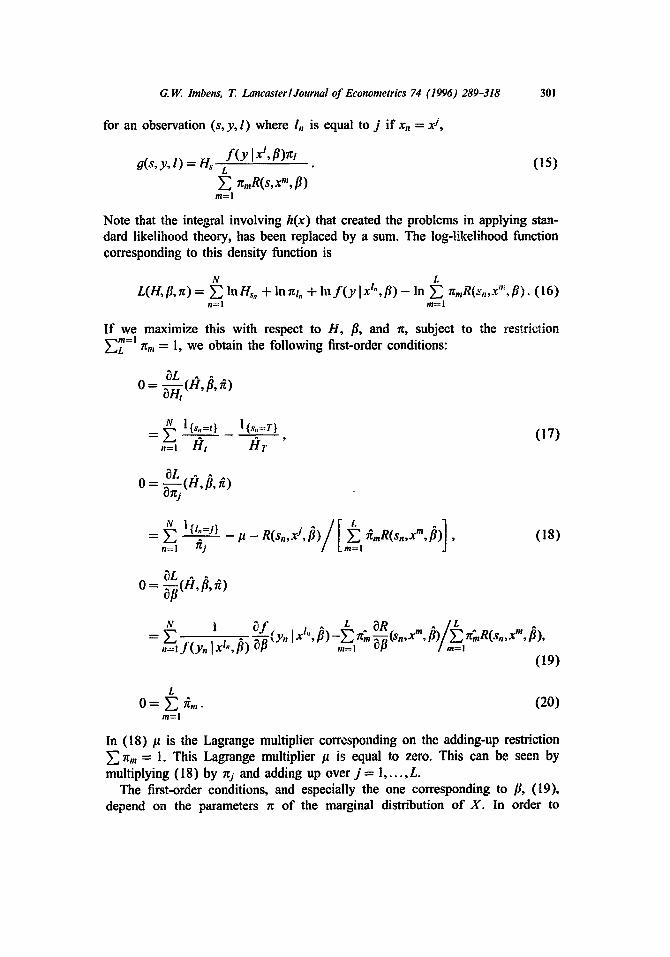
for an observation (s ,y, 1) where In is equal to j if xn = x J,

f ( y ix t, fl)g! g ( s , y , l ) = H s L

~zmR( s , x m, fl ) m=l

(15)

Note that the inte~al involving h(x) that created the problems in applying standard likelihood theory, has been replaced by a sum. The log-likelihood function corresponding to this density function is

N L L(H,p,~) = ~ lnHs,, + lnnl. + l n f ( y l x t " , p ) - In ~ nmR(s.,x'L[3). (16)

n=l m=!

If we maximize this with respect to H, fl, and ~, subject to the restriction ~ = 1 nm= 1, we obtain the following first-order conditions:

o= ~-~(n,~,~) N = ~ l{s.=t} l{s.=r} (17) .:I /~, /~T '

o= ~(~,,~,,~)

1 { t .= j } ^ ^

= ~ -2" 1~ -- R(sn,XJ, f l) ~zmR(sn,Xm, f l) , n=l 71:j m=l

(18)

~L ^ 0 = ~-~(H, fl, ~)

= )'~ - I " - ~ , Y n l . " L : O R . L . ^

n=I f ( y . Ix ", f l ) (19)

L o = ~ ~.,. (20)

m=l

In (18) ti is the Lagrange multiplier corresponding on the adding-up restriction E ll~m ----" 1. This Lagrange multiplier #x is equal to zero. This can be seen by multiplying (18) by 7rj and adding up over j = 1 . . . . . L.

The first-order conditions, and especially the one corresponding to fl, (19), depend on the parameters ~ of the marginal distribution of X. In order to

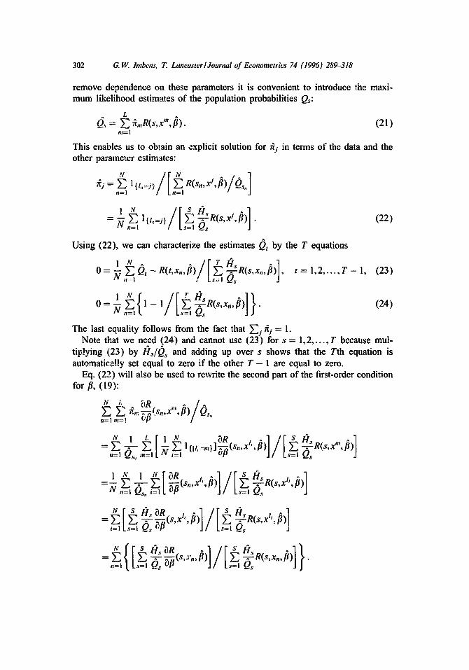
302 G.W. lmbens, T. Lancaster~Journal of Econometrics 74 (1996) 289-318

remove dependence on these parameters it is convenient to introduce the maximum likelihood estimates of the population probabilities Qs:

L Qs = E ~mRfs, xm, fl) • (21)

m=l

This enables us to obtain an explicit solution for ~j in terms of the data and the other parameter estimates:

~j = E l{l.=j} Rfsn,xJ, fl) . n=l

= N n=l ~ 1 {/.=j} Ls=l ~ s R(s,x ,//)] . (22)

Using (22), we can characterize the estimates Qt by the T equations ^

0 = ~l .=,~ Q , - R ( t , x . , ] ~ ) / [ s = , f ] HT~R(s'x"'fl)l'~2s J , = 1.2 . . . . . T - 1 , (23)

o=l ,~=l{ l - l / [ ,=~R(s , xn, fl)]}. (24)

The last equality follows from the fact that Y~; ~y = 1. Note that we need (24) and cannot use (23) for s = 1,2 . . . . . T because mul-

til;!ying (23) by fls/Qs and adding up over s shows that the Tth equation is automatically set equal to zero if the other T - 1 are equal to zero.

Eq. (22) will also be used to rewrite the second part of the first-order condition for r , (19):

N L L).~ ~ / ~_. ~_~ ~,n (Sn,X",fl) Qs,, n=l m=?

"' I'" °" ']/I 1 n=l ~ m=l i=l s=l

~R t,"

,,:, ,=, Q,

,.I / "

i=I z..,, I ~-e Ls=l Qs " J

n=l s=l ~-~s J OS

G.W. lmben~. T Lancasterl Journal of Econometrics 74 (1996) 289-318 303

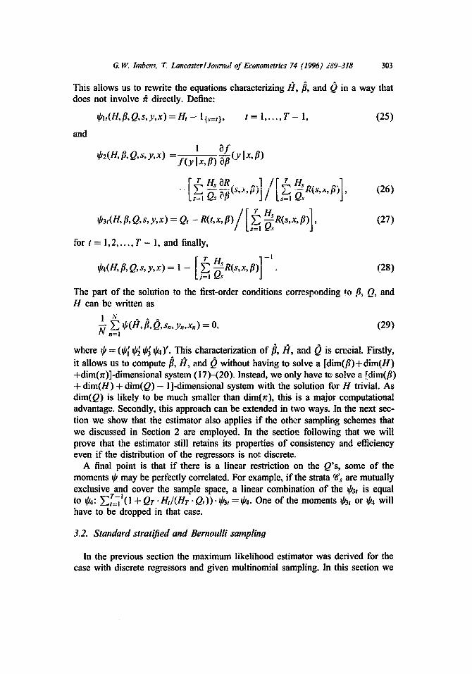
This allows us to rewrite the equations characterizing H,/~, and Q in a way that does not involve ~ directly. Define:

~lt(H, fl, Q , s , y , x ) = H t - l{s=t), t = 1 . . . . . T - 1, (25)

and

1 Of ~2(H,p ,Q,s ,y ,x ) - f ( y Ix, P) ~-fl(Y Ix, P)

-: ' (26)

rHs

for t = 1,2 . . . . . 7"- 1, and finally,

04(H, fl, O , s , y , x ) = 1 - - - R(s,x, fl) (28) j = l

The part of the solution to the first-order conditions corresponding to ,8, Q, and H can be written as

& ~ @(H, fl, O, Sn, Yn,Xn)=O, (29) At n=l

where ~ = ( ~ ~ ~ ~b4)'. This characterizatien of/~,/~, and 0 is crt:ciai. Firstly, it allows us to compute/~, H, and 0 without having to solve a [dim(fl)+dim(H) +dim(;r)]-dimensional system (17)-(20). Instead, we only have to, solve a [dim(p) + d im(H) + d im(Q) - 1]-dimensional system with the solution fiw H trivial. As dim(Q) is likely to be much smaller than dim(rr), this is a major computational advantage. Secondly, this approach can be extended in two ways. In the next section we show that the estimator also applies if the other sampling schemes that we discussed in Section 2 are employed. In the section following that we will prove that the estimator still retains its properties of consistency and efficiency even if the distribution of the regressors is not discrete.

A final point is that if there is a linear restriction on the Q's, some of the moments ~ may be perfectly correlated. For example, if the strata ~gs are mutually exclusive and cover the sample space, a linear combination of the ~ t is equal to ~b4: T-I ~'~t=l ( 1 + Qr" Ht / (Hr . Qt))" ~ t = ~'4. One of the moments ~ t or ~b4 will have to be dropped in that case.

3.2. Standard stratified and Bernoulli sampling

In the previous section the maximum likelihood estimator was derived for the case with discrete regressors and given multinomial sampling. In this section we

304 G. Hi bnbens. T. Lancaster~Journal o f Econometrics 74 (1996) 289 318

will show that if the regressors are discrete, but one of the other sampling schemes is employed, the estimator still has the same properties. In Section 2.2 it was shown that, conditional on s, the likelihood for the multinomial and the standard stratified sampling schemes were identical. Because the vector s is ancillary in both cases, the likelihood principle and the principle of conditionality imply that inference should be identical for both cases and be based on the conditional likelihood. In the previous section, however, we have been working with the full likelihoed based on the multinomial sampling scheme. Here we shall show that this does not matter.

Consider the log-likelihood function conditional on s for the discrete regressor case:

N L

L([I, re) = ~ In r~,,,, + In . f (y , I xl,,, fl) - In ~ rrmR(s,,,Xm, [I). tl=[ II1=1

(30)

Maximizing this over fl and ~ leads to first-order conditions identical to (18) and (19). Because the solution for [/ to (18) and (19) is the same as the solution for [I found by solving (29), the latter must equal the conditional maximum likelihood estimator for /I. I?t is in that case not to be interpreted as an estimator for H*, but as a ancillary statistic that simplifies calculation. The consequence of this is that no matter whether the sampling scheme is multinomial or standard stratified, the solution to (29) gives the correct estimator.

If the data are gathered with multinomial sampling, the asymptotic variance of the estimator for [J* can be calculated in a number of different ways. Firstly, one can interpret the estimator as maximizing the full likelihood function as given in (16). In that case one would calculate the asymptotic variance using the average outer product of the scores or the second derivatives of the log-likelihood function. Exactly the same estimates would be obtained using the conditional (on s) likelihood interpretation because the scores are identical tbr the two likelihood functions. Secondly, an estimate can be obtained by using the characterization in (29) and interpreting the estimator as a generalized method of moments estimator. There may be a difference between the two variance estimates in small samples but asymptotically they are identical. The GMM interpretation is convenient for computational reasons.

If we have standard stratified sampling, we can only use the conditional likelihood interpretation to get the asymptotic variance. But, as argued above, all asymptotic variance estimates must asymptotically be the same, and therefore the one obtained via the method of moments interpretation must also be valid for the fixed stratum size sampling scheme.

In Section 2.3 the Bernoulli sampling scheme was discussed. Now we have derived an efficient procedure for estimating H, Q, and fl for the multinomial sampling scheme, it is straightforward to derive an efficient estimator for that

G. IV.. 'rubens, T. LancasterlJournal of Econometrics 74 (1996) 289 318 305

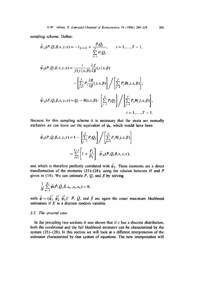
sampling scheme. Define:

~l,(P,Q, fl, s ,y ,x)= -l{s=,} + - - Pt Qt

T

E P Oj j= l

t = i . . . . . T - l ,

~2(p,Q, fl, s, y,x) - 1 ~ f

f (y [x, fl) -~(Y Ix'fl)

(b3t(P,Q, fl, s , y , x )=Qt -R( t , x , f l) '[j=~PJQJ]/[j=~PjR(j,x, fl)],

t = l . . . . . T - I .

Because for this sampling scheme it is necessary that the strata are mutually exclusive we can leave out the equivalent of ~b4, which would have been

= ~ 1 + • ~3t(e,o, fl, s,y,x), t=l

and which is therefore perfectly correlated with ~3. These moments are a direct transformation of the moments (25)-(28), using the relation between H and P given in (14). We can estimate P, Q, and fl by solving

1 ~b(P,Q, fl, s,,,vn,xn)=O, N ,=l

with ~ = (~'l ~2 ~'3)'. /5 ~, and [3 are again the exact maximum likelihood estimators if X is a discrete random variable.

3.3. Tile qcneral case

In the preceding two sections it was shown that if x has a discrete distribution, both the conditional and the full likelihood estimator can be characterized by the system (25)-(28). In this section we will look at a different interpretation of the estimator characterized by that system of equations. The new interpretation will

306 G.W. lmbens, T. Lancaster~Journal q]'Econometrk's 74 (1996) 289-318

validate the estimator for a much larger class of distributions for the explanatory variables than just discrete ones.

To reinterpret Eqs. (25)-(28), we go back to the multinomial sampling scheme with sampling density given by g(s ,y ,x ) in (4). We no longer assume a discrete distribution for X. Straightforward calculation shows that the expectation of ~(H, fl, Q,S, Y,X), evaluated at H*, Q*, and fl* equals zero (with the expectatio~ taken over the distribution induced by the sampling scheme). This implies that ~b is in general a valid moment in a generalized method of moments procedure. To ensure that solving (29) does indeed lead to a consistent and asymptotically normal estimator, we will make the following assumptions:

Assumption 3.2. For all s = 1 . . . . . T, Q*~ E (6, 1 - 6), H~* E (6, i - 6) Jbr some 6 > 0, fl* E intM, a compact subset o f ;~¢K, and x EiI', a compact subset o f .~f.

Assumption 3.3. f ( y Ix, fl) is a twice continuously differentiable function of fl for all fl E .~, and f and its first two deritatirc:; are continuous on ~q x :~'.

Assumption 3.4. The solution (H* Q* fl*) to E~b(H, fl, Q , s , y , x ) = O is unique.

Assumption 3.5. The expected outer product o f the moments, A0 = E~b(H*,fl*, Q*,s, y , x ) . ~b(H*,fl*,Q*,s, y ,x ) ' , is nonsinqular.

Assumption 3.6. The matrix o f first derivatives o f the moments, F0 = E[t3~b/ ~(n ' fl' Q' )](H*, I1", Q*, s, y, x), has ful l rank'.

Most of the assumptions are standard and require little discussion. Assumption 3.4 implies the parameters are identified. For this assumption to be satisfied, it is sufficient, but not necessary, that the parameters are identified given a random sample from any one of the strata. For example, often it is possible to estimate the parameters consistently given only a random sample from a truncated distribution. If the model is a standard normal linear model, all that would be required is that the covariance matrix of the regressors has full rank in at least one of the strata.

Betbre stating the formal results we will look at the case where exact prior information on H, fl, and or Q is available. Since most of the literature con- centrated almost exclusively on the estimation problem with Q and H known, this is clearly an important case to consider. An obvious way to deal with restrictions of this type is to go back to the discrete case and impose the restrictions at the level of the log-likelihood function (16). Maximizing (16) subject to the constraints would lead to a consistent and efficient estimator for the free parameters. That would be a very cumbersome way to derive restricted estimators. It would in particular be difficult to rewrite the equations characterizing the estimates in a way similar to (25)-(28). However, there is another way

G. W. lmbens, T. Lancaster~Journal of Econometrics 74 (1996) 289-318 301

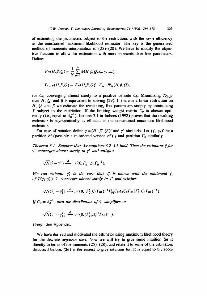
of estimating the parameters subject to the restrictions witb the same efficiency as the constrained maximum likelihood estimator. The key is the generalized method of moments interpretation of (25)-(28). We have to modify the objec- tive function to allow for estimation with more moments than free parameters. Define:

| N ~N(H. fl.Q) = -~ ~ ~b(H.fl .Q.s, .y, .x,) .

n=l

Tc,,,N(H, fl, Q) = JPN(H,~,Q)" C:v " ~v(H, fl, Q),

for CN converging almost surely to a positive definite Co. Minimizing Tcv,~ over H, Q, and B is equivalent to solving (29). If there is a linear restriction on H, Q, and fl we estimate the remaining, free parameters simply by minimizing T subject to the restriction. If the limiting weight matrix Co is chosen opti- mally (i.e., equal to Aol), Lemma 3.1 in lmbens (1992) proves that the resulting estimator is asymptotically as efficient as the constrained maximum likelihood estimator.

For ease of notation define 7 = (H' ff Q')' and 7" similarly. Let (~ 7~) ~ be a partition of (possibly a re-ordered version of) 7 and partition F0 similarly.

Theorem 3.1. Suppose that Assumpl'ions 3.2-3.5 hold. Then the estimator ~ for ~* converges almost surely to 7" and satisfies

v:N(:- 7*) d .,v.(o, ro, aor,o_~).

We can estimate 7~ in the case that 7~ is known with the minimand Yt o f T(yt, 7~ ). ~71 converoes almost surely to 7~ and satisfies

v~(:, - ~7) J, x(o, (r~, Coro~ )-trOt CoaoCoro~(r~t Coro~ )-~).

I f Co = Ao I. then the distribution o f ~t simplifies to

v:N(~ - ~;) d, ~:(o,(r6,~o,ro ~)_~).

Proof See Appendix.

We have derived and motivated the estimator using maximum likelihood theory for the discrete regressor case. Now we will try to give some intuition for it directly in terms of the moments (25)-(28), and relate it to some of the estimators discussed before. (26) is the easiest to give intuition for. It is equal to the score

308 G. W. lmbens, T. Lancaster/Journal oJ" Econometrics 74 (1996) 289-318

for the conditional likelihood of Y and S given X. 2 The second set of moments extracts information from the marginal distribution of X. The restriction on Q in the population is

Q.~. = EpR(s ,x , fl) = f t . : R(s ,x , f l ) f ( x ) d x ,

which translates into

Q.~ = EsR(s,x ,[3) . b ( H , Q , ~ , x ) = f c: R(s ,x ,[J) . b (H ,Q , [3 , x )o (x )dx ,

where the subscripts p and s denote expectations taken over the population and sample distributions, respectively, and b(.) is the bias function given in (!1). (27) i~ the moment corresponding to this expectation.

More difficult to explain is the role of (25). If H is unknown, this moment corresponds to the score for H, and its role is clear. Even if H is known, the presence of this moment is important despite the fact that in that case the moment does not contain any unknown parameters. Its influence works through its effect on the weight matrix in the method of moments procedure. In other words, it depends on the correlation between (25) and the other moments. An ana- logy is Seemingly Unrelated Regression where the same phenomenon can occur. Lancaster (1990) gives some intuition by showing that the presence of this moment ensures that the estimator is conditional on the ancillary statistic Ns. A different derivation of these moments for the discrete choice case, providing additional intuition, is given in Lancaster and Imbens (1991).

The derivation of the estimator, using maximum likelihood estimation for a particular parametrization and then generalizing the applicability to a larger class of problems, suggests that the estimator is efficient. Chamberlain (1987) extends a definition of efficiency, local asymptotic minimax, to this type of semiparametric problem. An alternative semiparametric efficiency concept developed by Begun et al. (1984) and discussed in Newey (1990) is applied to estimators for choice- based sampling by Imbens (1992). In that framework we look at the supremum of all Cram6r-Rao lower bounds for parametric models that include the true model. In this case we already have a candidate for the supremum and an estimator that attains the candidate bound. We therefore only have to show that there is a sequence of Cram6r-Rao bounds that does converge to this proposed bound. We do so by constructing a partition of the ?/" space into L nonoverlapping subsets, .°l't, with the unknown parameters fit = Pr(x E flt'l)= f..l, h(z )dz . We then let

2 The conditional likelihood, based on the conditional density given in (7), is equal to

L([~) = In H~,, - In Q~,, + In f(yn Ixn,[~1) - In ~ R(t,x,,,[~). n=:l t = l

G.W. lmbens, T. Lancasterl Journal of Econometrics 74 (1996) 289-318 309

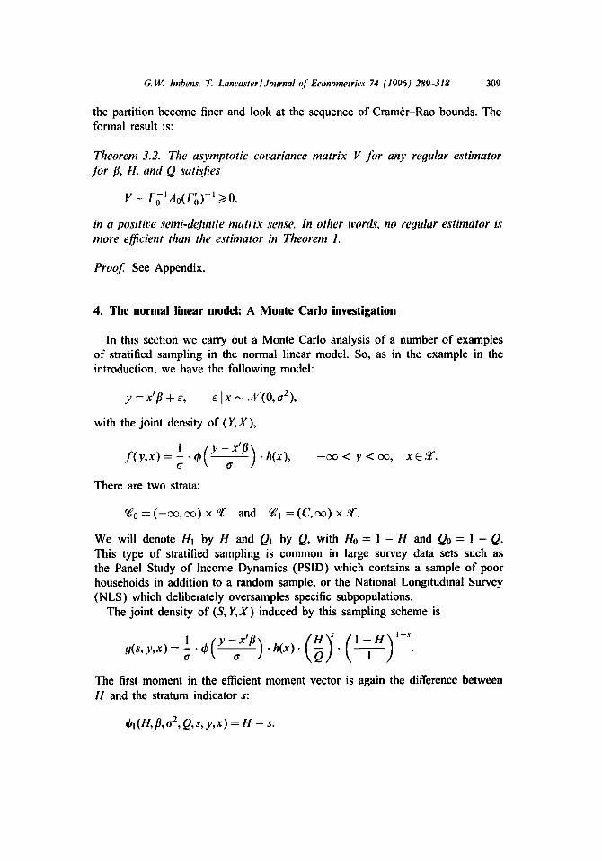
the partition become finer and look at the sequence of Cram6r-Rao bounds. The formal result is:

Theorem 3.2. The asympto t ic covariance m a t r i x V f o r any regular es t imator

f o r l~, H, and Q satisfies

z - r o ~ A O ( r ' o ) -~ >>.o,

in a posi t ive semi-defini te m a t r i x sense. In other words, no regular es t imator is

more efficient than the es t imator in Theorem 1.

Proof. See Appendix.

4. The normal linear model: A Monte Carlo investigation

In this section we carry out a Monte Carlo analysis of a number of examples of stratified sampling in the normal linear model. So, as in the example in the introduction, we have the following model:

y = x ' f l + e, e Ix . . . . ~P(O, a 2 ),

with the joint density of (Y,X),

- - . ,

f ( y , x ) = tr - c ~ < y < c~, x 6 :[.

There are two strata:

~ 0 = ( - o e , c~)x.°/" and cWl=(C, oo) x.~.

We will denote Hi by H and Ql by Q, with H0 = 1 - H and Q0 = 1 - Q . This type of stratified sampling is common in large survey data sets such as the Panel Study of Income Dynamics (PSID) which contains a sample of poor households in addition to a random sample, or the National Longitudinal Survey (NLS) which deliberately oversamples specific subpopulations.

The joint density of (S, Y , X ) induced by this sampling scheme is

g(s, y , x ) = - • (~ • h (x ) . • t7

The first moment in the efficient moment vector is again the difference between H and the stratum indicator s:

~Ot(H,[3, a z, Q , s , y , x ) = H - s.

310 G. I'E lmbens. T. LancasterlJournal of Econometrics 74 (1996) 289 318

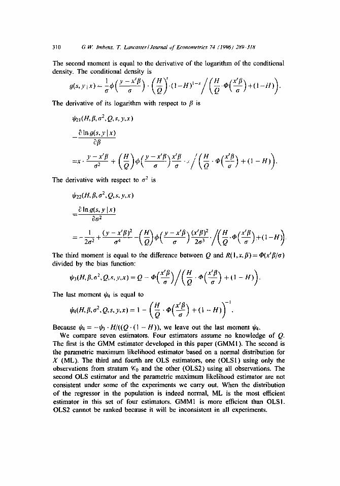
The second moment is equal to the derivative of the logarithm of the conditional density. The conditional density is

y H s

The derivative of its logarithm with respect to fl is

~l(H, fl, a2,Q,s, y,x)

~lno(s, ylx) eft

y - x ' f l ( H ~ b ( y - x ' f l ) x ' [ 3 / ( H (x__aft_) ) =x. \ O / C - - g - - . - - g - " + ( l - n ) .

The derivative with respect to 62 is

~b22( H, fl, aZ, Q, s, y,x )

~3 lno(s,y Ix) ~a 2

H , / y -x ' f l , ( x t f l ) 2 . q~ (x~_~_~) _i_ ( 1 I (Y-X'[3)2 ( - Q ) q ) , ~ j ~ . / ( Q -HO. - - 26 ~ -I- 6 4

The third moment is equal to the difference between Q and R( I,x, [3)= q~(x'[3/a) divided by the bias function:

H ~O3(,,[3,02,Q,s,y,x)=Q - q ~ ( ~ - ~ - ) / ( ~ - q ~ ( ~ - ~ ) + ( 1 - H ) ) .

The last moment if4 is equal to

) ~04(H,[3,a2,Q,s,y,x)= i - .q~ + ( 1 - H ) .

Because ~b4 = - ~ . H/((Q. (! - H ) ) , we leave out the last moment ~4. We compare seven estimators. Four estimators assume no knowledge of Q.

The first is the GMM estimator developed in this paper (GMMI). The second is the parametric maximum likelihood estimator based on a normal distribution for X (ML). The third and fourth are OLS estimators, one (OLSI) using only the observations from stratum % and the other (OLS2) using all observations. The second OLS estimator and the parametric maximum likelihood estimator are not consistent under some of the experiments we carry out. When the distribution of the regressor in the population is indeed normal, ML is the most efficient estimator in this set of four estimators. GMMI is more efficient than OLSI. OLS2 cannot be ranked because it will be inconsistent in all experiments.

G. W. Imbens, T. Lancaster/Journal o f Econometrics 74 (1996) 289 318 311

The three estimators that do require knowledge of Q are the optimal GMM estimator (GMM2), the conditional maximum likelihood estimator (CML), and the weighted maximum likelihood estimator (WML). The CML estimator is based on solving

N p([i, a 2 ) = Y]~ d/2( H, l:l, a2, Q,s, y , x ) = O.

n=l

Because without stratified sampling the maximum likelihood estimator would be least squares, the WML estimator is weighted least squares with weights

wn \ l - t t J " H + ( I - H ) . Q "

where 6(-) is the indicator function. WML and CML are both more efficient than OLSI, but less than GMM2. They cannot in general be ranked relative to GMMI or ML. GMM2 is more efficient than GMMI, but cannot be ranked relative to ML.

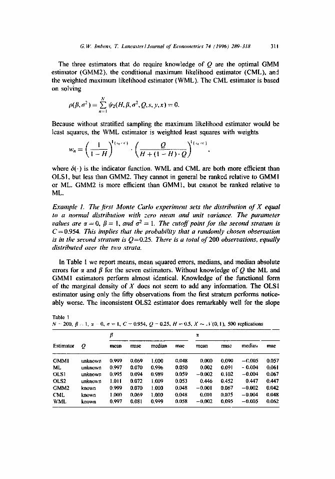
Example 1. The first Monte Carlo experhnent sets the distribution o f X equal to a normal distribution with zero mean and unit variance. The parameter values are ~ = 0,/~ = !, and a 2 = 1. The cutoff point for the second stratum is C = 0.954. This implies that the probability that a randomly chosen observation is in the second stratum is Q=0.25. There is a total of 200 observations, equally distributed over the two .strata.

In Table 1 we report means, mean squared errors, medians, and median absolute errors for ~ and fl for the seven estimators. Without knowledge of Q the ML and GMMI estimators perform almost identical. Knowledge of the functional form of the marginal density of X does not seem to add any information. The OLSi estimator using only the fifty observations from the first stratum performs notice- ably worse. The inconsistent OLS2 estimator does remarkably well for the slope

Table I N = 200, fl = I, ~ = 0, a = I, C = 0.954, Q = 0.25, H = 0.5, X ..... t (0, I ), 500 replications

Estimator Q mean rinse median mac mean rms¢ media,,, mac

GMM I unknown 0.999 0.069 1.000 0.048 0.000 0.090 -P,.005 0.057 ML unknown 0.997 0.070 0.996 0.050 0.002 0.091 - 0.004 0.061 OLS I unknown 0.995 0.094 0.989 0.059 -0.002 0.102 -0.004 0.067 OLS2 unknown 1 . 0 1 1 0.072 1.009 0.053 0.446 0.452 0.447 0.447 GMM2 known 0.999 0.070 1.000 0.048 -0.001 0.067 -0.002 0.042 CML known 1.000 0.069 1.000 0.048 0.001 0.075 -0.004 0.048 WML known 0.997 0.081 0.999 0.058 -0.002 0.095 -0.005 0.062

312 G.W. hnbens. 12. Lancaster~Journal of Econometrics 74 (i996) 289-318

coefficient. The bias of the intercept is large, but the increase in precision leads to a lower root mean squared error for the slope coefficient compared to OLSI.

Knowledge of Q leads to sizable gains in the precision of the estimator for the intercept (cf. GMM2 and GMMI ) but no perceptible gain in precision for the slope coefficient. This is reminiscent of results in choice-based sampling where in logit models it can be shown that knowledge of marginal shares affects only precision in intercepts but not precision of slope coefficients. In this experiment the maximum conditional likelihood estimator performs marginally better than the weighted estimator.

It is also interesting to compare OLS 1 and WLS. WLS is more efficient because it uses the second subsample, even if not in a fully efficient way. In this setup there is only a modest gain from using the observations from the stratum ~l relative to not using them at all.

From the results presented in Table ! we can also compare the efficiency of the estimators relative to a completely random sample of size 200 by dividing the rmse and mae for OLSI by v ~ to get 0.066 and 0042, respectively. This shows that we would have been better off with a completely random sample of size 200 than with a augmented sample with 10e observations randomly drawn and 100 observations from the stratum cg~.

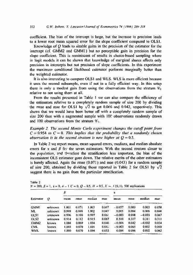
Example 2. The second Monte Carlo experiment changes the cutoff point from C---0.954 to C = O. This implies that the probability that a randomly chosen observation is in the second stratum is now higher at Q = 0.5.

In Table 2 we report means, mean squared errors, medians, and median absolute errors for ~ and fl fe~" the seven estimators. With the second stratum closer to the population, and therefore the stratification less important, the bias of the inconsistent OLS estimator goes down. The relative merits of the other estimators is barely affected. Again the rinse (0.071) and mae (0.043) for a random sample of size 200, obtained by dividing those reported in Table 2 for OLSI by v/2 suggest there is no gain from the particular stratification.

Table 2 N = 200, fl = I, :t -- 0, o = I C = O, Q = 0.5, H = 0.5, X ~,. I "(0, I ), 500 replications

Estimator Q mean rinse median mac mean m~se median mac

GMM ! unknown 1 . 0 0 1 0.071 1.003 0.047 -0.057 0.080 0.003 0.058 ML unknown 0.999 0.069 1.002 0.047 0.005 0.084 0.006 0.060 OLSI unknown 0.996 0.100 0.997 0.0o] -0.003 0.098 -0.003 0.067 OLS2 unknown 0.914 0.112 0.915 0.087 0.310 0.317 0.311 0.311 GMM2 known 1.004 0.069 1.004 0.046 -0.006 0.042 -0.002 0.034 CML known 1.003 0.070 I.OOI 0.04.3 -0.003 0.065 0.002 0.048 WML known 1.000 0.070 1.004 0.053 0.004 0.086 0.002 0.062

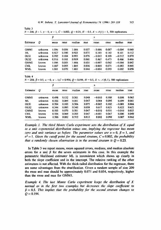
G. W. lmbens. T. Lancaster~Journal of Econometrics 74 (1996) 289-318

Table 3 N = 2 0 0 , f l = I , ~t = 0 , a = 1, C = 0 . 8 0 2 , Q = 0 . 2 5 , H = 0 . 5 , X --~ t~( 1 ) - I, 500 replications

313

Estimator Q mean rinse median mae mean rmse median mae

GMMI unknown 1.006 0.056 1.006 0.037 -0.006 0.087 -0.004 0.060 ML unknown 0.927 0.100 0.923 0.075 0.103 0.143 0.101 0.112 OLS1 unknown 0.992 0.104 0.993 0.076 -0.012 0.103 -0.012 0.070 OLS2 unknown 0.916 0. l01 0.919 0.081 0.467 0.473 0.466 0.466 GMM2 known 1.006 0.055 1.006 0.035 -0.007 0.062 -0.004 0.042 CML known 1.007 0.055 1.005 0.036 -0.005 0.071 -0.002 0.045 WML known 1.001 0.070 1.003 0.044 -0.004 0.093 0.002 0.058

Table 4 N = 200, fl = 0.5, ~t = 0, cr = I,C = 0.954, Q = 0.194, H = 0.5, X -,,, if(0, I ), 500 r e p l i c a t i o n s

Estimator Q mean rmse median mac mean rmsc median mac

GMMI unknown 0.498 0.132 0.501 0.048 -0.010 0.188 0.008 0.062

ML unknown 0.503 0.069 0.501 0,047 0.004 0.095 0.009 0.061 OLS I unknown 0.504 0.103 0.506 0.073 -0.002 0.102 -0.001 0.066 OLS2 unknown 0.544 0.085 0.545 0.058 0.617 0.621 0.622 0.622 GMM2 known 0.503 0.070 0.501 0.047 -0.010 0.051 -0.010 0.033 CML known 0.504 0.069 0.503 0.047 -0.001 0.067 0.000 0.040 WML known 0.506 0.082 0.512 0.053 0.002 0.098 0.007 0.062

Example 3. The third Monte Carlo experiment sets the distribution of X equal to a unii exponential distribution minus one, implying the regressor has mean zero and unit variance as before. The parameter values are oc = 0, fl = 1, and ~2 = I. Given the cutoff point for the second stratum, C = 0.802, the probability that a randomly chosen observation is in the ,second stratum is Q = 0.25.

In Table 3 we report means, mean squared errors, medians, and median absolute errors for g and fl for the seven estimators in this case. In this example the parametric likelihood estimator ML is inconsistent which shows up clearly in both the slope coefficient and in the intercept. The relative ranking of the other estimators is not affected. With the thick-tailed distribution for the regressor, there are some advantages from the stratification. Given a random sample of size 200 the rmse and mac should be approximately 0.071 and 0.054, respectively, higher than the rmse and mae for GMMI.

Example 4. The last Monte Carlo experiment keeps the distribution of X normal as in the .first two examples but decreases the slope coefficient to fl = 0.5. This implies that the probability Jbr the second stratum changes to Q = 0.194.

314 G. 15: bnbens, T. Lancaster/JounTal t e Econometrics 74 (1996) 289.-318

In Table 4 we report means, mean squared errors, medians, and median absolute errors for ~ and fl for the seven estimators for this scenario. With the slope coefficient smaller, the stratum c~l has smaller probability in the population. This makes the stratified sample more information than a random sample of the same size. The gain of actually using the second stratum by weighting (WLS) relative to only using the random subsample (OLSI) is now much larger than in the previous setups.

Overall the simulations lead to a number of tentative conclusions. First, the GMM estimators perform well relative to the full likelihood estimator. If the marginal distribution of the regressors is correctly specified, there is Iittle loss of precision from not using it and instead usinlz the GMM estimators. If on the other hand the distribution of the regressors is misspecified, there can be a considerable bias for the ML estimator. There is therefore no reason to use the parametric likelihood estimator. Its potential gains when correctly specified are small compared to the potc~ltial losses when misspecified.

Second, the gain in precision from knowledge of the stratum probabilities is largely confined to the intercept, similar to conclusions in choice-based sampling.

Third, the conditional maximum likelihood estimator seems to be slightly better than the weighted least squares estimator. ~-lowever, the weighted least squares estimator is clearly better than the other 'simple' estimators, i.e., estimators that require little additional programming beyond implementing programs for random samples, OLSI and OLS2.

Fourth, the smaller the marginal probability of the strata, the more informative a stratified sample is relative to a random sample of the same size. In other words, given fixed strata, the smaller in absolute value the slope coefficients, the more informative a stratified sample.

These simulations suggest that in practice the choice should be between the efficient GMM estimators or the inefficient, but computationally simpler WLS estimator. On the one hand is the computational ease of the WLS estimator, which only requires introducing weights into the same estimation procedure that would be used if the researcher had a random sample from the population, compared to the efficient GMM estimator, which requires programming of the modified moment functions and even in simple examples numerical optimization. On the other hand is the e~ciency loss of the WLS estimator, which in these examples is between 20 and 40% of the variance of the efficient estimator.

5. Conclusion

In this paper we study the problem of estimating parameters of the conditional distribution if the sampling is stratified. Stratified sampling schemes can be im- plemented in a number of ways. We discuss three common types and show that they can be analyzed in a unified manner. We then derive an estimator for the

G.W. hnbens, T. Lancaster~Journal of Econometrics 74 (1996)289-318 315

general case. The procedure used to derive the estimator is similar to that proposed by lmbens (1992) for choice-based sampling. The estimator we propose is a computationally simple, generalized method of moments estimator. We show that the estimator is efficient using semi-parametric efficiency bounds proposed by Begun et al. (1983).

A Monte Carlo experiment shows that the estimator has good properties in moderately sized samples. This experiment also indicates that the gains of using fully parametric models are small relative to the losses due to potential misspec- ification. Finally, knowledge of stratum probabilities seems relevant mainly for estimating intercepts rather than the typically more interesting slope coefficients.

Appendix: Proofs of Theorems 3.1 and 3.2

Proof of Theorem 3.1 The assumptions made, (2.1)-(2.2) and (3.2)-(3.3), guarantee the conditions

needed fbr standard theorems on generalized method of moments estimation to hold. See for an extensive discussion and reference Hansen (1982) and Newey and McFadden (1994). ~d~,~

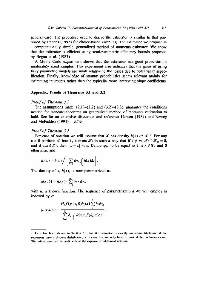
Proof of Theorem 3.2 For ease of notation we will assume that X has density h(x) on :~'. 3 For any

e. > 0 partition : f into L,: subsets :g't in such a way that if ! ~ m, :?ft N ~m = 0, and i fx , zE: f t , then ] x - z I <e.. Define ~bl.~ to be equal to 1 i f x E . f t and 0 otherwise, and

:~'!

The density of x, h(x), is now parametrized as

L h(x; 6) = h,:(x) • ~ 61" 4~/.~,

I=1

with h,: a known function. The sequence of parametrizations we will employ is indexed by ~::

HJ' (y Ix, ~)h,:(x) ~ 6tdptx I

O,:(s,i,x)= L, 6t f R(s,z,/~)h,:(z)cL-

I= I .fl

3 As it has been shown in Section 3.1 that the estimator is exactly maximum likelihood if the regressors have a discrete distribution, it is clear that we only have to look at the continuous case. The mixed case can be dealt with at the expense of additional notation.

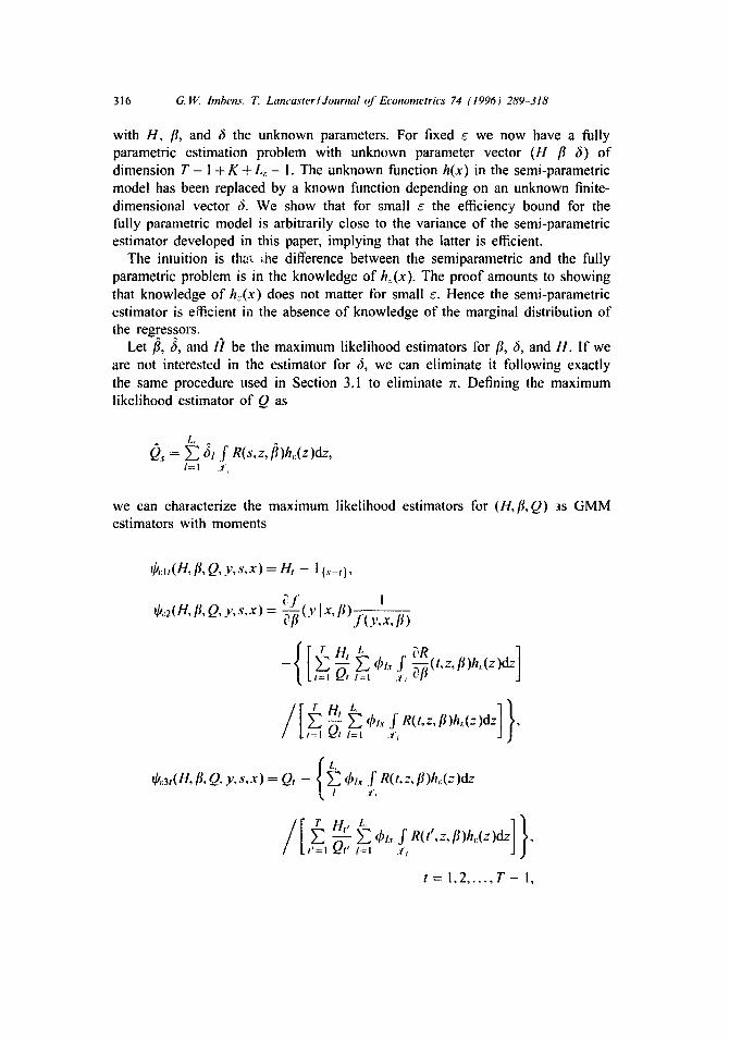
316 G.W. hnbens, T. Lain'aster I Journal of Econometrics 74 (1996) 289 318

with H, fl, and 6 the unknown parameters. For fixed e we now have a fully parametric estimation problem with unknown parameter vector (H fl 6) of dimension T - 1 + K + L, : - I. The unknown function h(x) in the semi-parametric model has been replaced by a known function depending on an unknown finite- dimensional vector 6. We show that for small e the efficiency bound for the fully parametric model is arbitrarily close to the variance of the semi-parametric estimator developed in this paper, implying that the latter is efficient.

The intuition is that tile difference between the semiparametric and the fully parametric problem is in the knowledge of h~(x). The proof amounts to showing that knowledge of h~(x) does not matter for small e. Hence the semi-parametric estimator is efficient in the absence of knowledge of the marginal distribution of the regressors.

Let fl, 6, and/-) be the maximum likelihood estimators for fl, 6, and H. If we are not interested in the estimator for 6, we can eliminate it following exactly the same procedure used in Section 3.1 to eliminate ft. Defining the maximum likelihood estimator of Q as

L ^

O, = g 6, .f I=1 .t;

we can characterize the maximum likelihood estimators for (H, fl, Q) as GMM estimators with moments

~b,:z,( H, fl, Q, y , s , x ) =

~k~:2(H, fl, Q, y , s , x ) =

~:3t( H, fl, Q, y , s , x ) =

H t - ll.,.=t },

{~ .I" {~-~- (y Ix,/~) l,(y/,/~)

/4 . L ,~

I=I .lJ

,=,-~t ~" ~L, f R(t,z, fl)h,:(z)dz , /=1 ,1"~

Qt-{~l~blx'rR(t 'z ' f l)h':(z)dz. ,r ,

/ [ , ]} H,__, E ~lx f R(t ' ,z, fl)h,:(z)cL ~ • F = I ~ 'F /=1 . t ' I

t = !,2 . . . . . T - I,

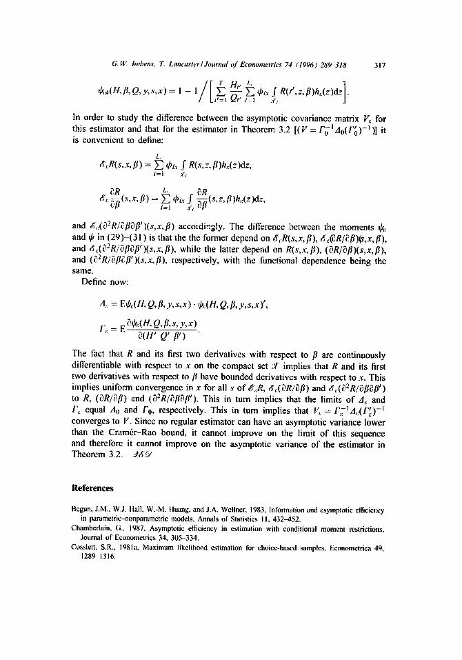
G. W. Imbens, 7". Lancaster/Journal o f Econometrk's 74 (1996) 289318 317

~b~:4(H, fl, Q, y , s , x ) = I - i Ht___~, ~ d?lx f R ( t t , z , f l )hr . ( z )dz . / / = l Qt, I = l .t'l

In order to study the difference between the asymptotic covariance matrix E. for this estimator and that for the estimator in Theorem 3.2 [(V = FolAo(F~)-l)] it is convenient to define:

L ~,:R(s,x,l~) = ~ ~x f R(s,z.#)h~(z)dz,

1= I .'f l

d' JR s x L, JR , :~( , ,t~) = E ~,x f ~(s,~,t~)h,:(z)dz, /=1 .~'!

and ~',:(J2R/j[lOff)(s,x, fl) accoTdingly. The difference between the moments ~b~: and ~b in (29)-(31) is that the the former depend on g,:R(s,x, fl), .~,:(dR/~[J)~,x, fl), and e~,:(O2R/jfl~fl')(s,x, fl), while the latter depend on R(s,x, fl), (OR/~fl)(s,x, fl), and (j2R/~[h3fl')(s,x, fl), respectively, with the functional dependence being the same.

Define now:

A,: = E~,:(H,Q, fl, y , s ,x ) . ~:(H,Q, fl, y ,s ,x) ' ,

I',: = E ~,:(H,Q, fl, s,Y, x) ~(H' Q ' / / ' )

The fact that R and its first two derivatives with respect to fl are continuously differentiable with respect to x on the compact set :1" implies that R and its first two derivatives with respect to fl have bounded derivatives with respect to x. This implies uniform convergence in x for all s of ~,:R, 6",:(JR/Jfl) and d,:(~2R/JflJfl') to R, (JR/~fl) and (~2R/jflJfl'). This in turn implies that the limits of A,: and F,: equal A0 and F0, respectively. This in turn implies that V,: = FT. IA,:(F') -I converges to V. Since no regular estimator can have an asymptotic variance lower than the Cramrr-Rao bound, it cannot improve on the limit of this sequence and therefore it cannot improve on the asymptotic variance of the estimator in Theorem 3.2. ~6 '~

References

Begun, J.M., W.J. Hall, W.-M. Huang, and J.A. Wellner, 1983, Information and asymptotic efficiel:cy in parametric-nonparametric models, Annals of Statistics I I, 432-452.

Chamberlain, G., 1987, Asymptotic efficiency in estimation with conditional moment restrictions, Journal of Econometrics 34, 305-334.

Cosslett, S.R., 1981a, Maximum likelihood estimation for choice-based samples, Econometrica 49, 1289-1316.

318 G. W. Imbens, T. Lancaster l Journal of Econometrics 74 (1996) 289-318

Cosslett, S.R., 1981b, Efficient estimation of discrete choice models, in: C.F. Manski and D. McFadden, eds., Structural analysis of discrete data with econometric applications (MIT Press, Cambridge, MA).

Cox, D.R. and D. Hinkley, 1974, Theoretical statistics (Chapman and Hall, London). Engle, R., D. Hendry, and J.F. Richard, 1983, Exogeneity, E~:onometrica 51, 277-304. Gill, R.D., Y. Vardi, and J.A. Wellner, 1988, Large sample theory of empirical distributions in biased

sampling models, Annals of Statistics 16, 1069-1112. Hansen, L.P., 1982, Large sample properties of generalized method of moment estimators,

Econometrica 50, 1029-1054. Hausman, J.A., and D. Wise, 1981, Stratification on endogenous variables and estimation: The Gary

income maintenance experiment, in: C. Manski and D. McFadden, eds., Structural analysis of discrete data with econometric applications (M1T Press, Cambridge MA).

Hsieh, D.A., C.F. Manski, and D. McFadden, 1985, Estimation of response probabilities from augmented retrospective observations, Journal of thz American Statistical Association 80, 651- 662.

Imbens, G.W., 1992, An efficient method of moments estimator for discrete choice models with choice-based sampling, Econometrica 60, 1187-1214.

Jewell, N., 1985, Least squares regression with data arising from stratified samples of the dependent variable, Biometrika 72, 11-21.

Kalbfleisch, J.D. and J.F. Lawless, 1988, Estimation of reliability in field performance studies, Technometrics 30, 365-388.

Lancaster, T , 1990, A paradox in choice-based sampling, Department of Economics working paper (Brown University, Providence, RI).

Lancaster, T., and G.W. lmbens, 1990, Choice-based sampling of dynamic populations, in: Hartog, Ridder, and Theeuwes, eds., Panel data and labor market studies.

Lancaster, T., and G.W. Imbens, 1991, Choice-based sampling: Inference and optimality, Department of Economics working paper (Brown University, Providence, RI).

Manski, C.F. and S.R. Lerman, 1977, The estimation of choice probabilities from choice-based samples, Econometrica 45, 1977-1988.

Manski, C.F. and D. McFadden, 1981, Alternative estimators and sample designs for discrete choice analysis, in: C.F. Manski and D. McFadden, eds., Structural analysis of discrete data with econometric applications (MIT Press, Cambridge, MA).

Newey, W., 1985. Maximum likelihood specification testing and conditional moment tests, Econometrica 53, 1047-1069.

Newey, W., 1990, Semiparametric efficiency bounds, Journal of Applied Econometrics 5, 99-135. Newey, W. and D. McFadden, 1994, Estimation in large samples and hypothesis testing, in: R. Engle

and D. MacFadden, eds., Handbook of econometrics, Vol. 4 (North-Holland, Amsterdam).

Documents

JOURNAL OF Econometrics Efficient estimation and ... · Econometrics Efficient estimation and stratified sampling ... The complications arise if we have both ... We are interested