Efficient Sensitivity Analysis ofMortgage Backed Securities

Jian ChenFannie Mae

The Robert H. Smith School of BusinessUniversity of Maryland

College Park, MD 20742-1815jchen@rhsmith.umd.edu

fax: (202) 752-0138

Michael C. FuThe Robert H. Smith School of Business

University of MarylandCollege Park, MD 20742-1815

mfu@rhsmith.umd.edufax: (707) 897-3774

December 2001

1

Abstract

Because of the complicated behavior of their cash flows, mortgage-backedsecurities (MBS) are almost always priced using Monte Carlo simulation. Sensitivityanalysis is a critical component of these simulations. Risk managers need these numbersto hedge their exposure to interest risk and prepayment risk. In order to carry this out in acomputationally efficient manner, we derive perturbation analysis (PA) gradientestimators in a general setting, without restrictions to any specific interest rate model orprepayment model. Then we apply the estimators to the Hull-White interest rate modeland a common prepayment model to derive the corresponding specific PA gradientestimators, assuming the shock of interest rate term structure takes the form of a Fourier-like harmonic series. Numerical experiments comparing finite difference (FD) gradientestimators with our PA estimators indicate that the PA estimators can provide betteraccuracy than FD estimators while using much lower computational cost. In the test caseof 5 duration and 25 convexity estimators, the computational time is reduced by 97.2%.Using the estimators, we analyze the impact of term structure shifts on various mortgageproducts. Based on insights gained from the analysis, we propose a new product thatcould potentially benefit mortgage borrowers and investors.

Keywords: Mortgage Backed Securities, Risk Management, Monte Carlosimulation, Perturbation Analysis, Gradient Estimation.

2

1 Introduction

A mortgage-backed security (MBS) is a security collateralized by residential orcommercial mortgage loans. An MBS is generally securitized, guaranteed and issued bythree major MBS originating agencies: Ginnie Mae, Fannie Mae, and Freddie Mac. Thecash flow of an MBS is generally the collected payment from the mortgage borrower,after the deduction of servicing and guaranty fees. However, the cash flows of an MBSare not as stable as that of a government or corporate coupon bond. Because the mortgageborrower has the prepayment option, mainly exercised when moving or refinancing, anMBS investor is actually writing a call option. Furthermore, the mortgage borrower alsohas the default option, which is likely to be exercised when the property value dropsbelow the mortgage balance, and continuing mortgage payments would not makeeconomical sense. In this case the guarantor is writing the borrower a put option, and theguarantor absorbs the cost. However, the borrower does not always exercise the optionswhenever it is financially optimal to do so, because there are always non-monetaryfactors associated with the home, like shelter, sense of stability, etc. And it is also veryhard for the borrower to tell whether it is financially optimal to exercise these optionsbecause of lack of complete and unbiased information, e.g., they may not be able toobtain an accurate home price, unless they are selling it. And there are also some otherfixed/variable costs associated with these options, such as the commission paid to the realestate agent, the cost to initialize another loan, and the negative credit rating impact whenthe borrower defaults on a mortgage. All these factors contribute to the complexity ofMBS cash flows. In practice, the cash flows are generally projected by complicatedprepayment models, which are based on statistical estimation on large historical data sets.Because of the complicated behaviors of the MBS cash flow, due to the complexrelationships with the underlying interest rate term structures, and path dependencies inprepayment behaviors, Monte Carlo simulation is the generally only applicable method toprice MBS.

Associated with the uncertainty of cash flows are different kinds of risks.Treasury bonds only bear interest rate risk, whereas non-callable corporate bonds carryinterest rate and credit risk. MBS are further complicated by prepayment risk (resultingfrom both prepayment and default). Thus risk management is especially critical forportfolios with large holdings in MBS. Duration and convexity are mainly the riskmeasurements for fixed income portfolio mangers. Many practitioners use either theMacaulay duration, or modified duration (Robert Kopprasch [1987]) to capture the MBSprice sensitivity w.r.t. interest rate changes, but these assume a constant yield and knowndeterministic prepayment pattern, which is rarely the case in practice. So these twoapproaches to calculate duration can lead to serious errors when used in hedging. BennettW. Golub [2001] proposed four different approaches to get the duration: Percent of Price(POP), Option-Adjusted Duration (OAD), Implied Duration, and Coupon Curve Duration(CCD). The first two approaches apply parallel shifts in the yield curve, which is not avery realistic assumption. The latter two approaches require large numbers of previous orcurrent accurate MBS prices that are comparable to the MBS whose duration is to bemeasured. This might not be practical for on-the-fly pricing and sensitivity analysis.

3

Another drawback of these approaches is that they handle only duration and convexity(delta and gamma), but not sensitivity to interest rate volatility (vega). OAD can estimatethe vega using a finite difference method, which requires 3 simulations to estimate onegradient: the base, up and down cases. And non-parallel yield curve shifts require moreparameters to characterize the shift. Thus, in the setting we consider, to estimate theduration w.r.t. yield curve shift of 4 summed harmonic functions would require 9 (2n+1,n=4) simulations. To estimate vega requires 2 additional simulations. So estimating theduration and vega roughly increases the computational cost by a factor of 10. Calculatingconvexity would require 75 duration estimators to calculate 25 convexity estimators,increasing the simulation factor to 225. In other words, if one were to use 10,000replications to estimate the MBS price, over 2.25 million simulations would be requiredto estimate the various sensitivities. Our work aims to decrease this computational burdendramatically.

Most literature on MBS has concentrated on prepayment model estimations,although some of the recent work has focused on computational efficiency, e.g.,dimensionality reduction via Brownian bridge (Caflisch et al. [1997]), and quasi-MonteCarlo (Åkesson and Lehoczky [2000]). However, there is no work that we are aware ofthat addresses efficient sensitivity analysis of MBS pricing and hedging. Related work inequities includes Fu and Hu[1995], Broadie and Glasserman [1996], Fu et al. [2000],[2001], and Wu and Fu [2001]. Perhaps the most relevant paper to our work isGlasserman [1999], “Fast Greeks in Forward LIBOR Model”, which applied perturbationanalysis (PA) method for caplet price sensitivity analysis. Yet most of these modelsinvolve only a single exercise decision with a one-time payoff, whereas an MBS is a poolof homogenous mortgages rather than an individual mortgage loan. So the cash flowsexist until the maturity of the collateral, and they are highly path dependent, which makessensitivity analysis of MBS more complicated.

The other relevant body of research literature analyzes the duration of differentmortgage products. We know that adjustable rate mortgage (ARM) products will have adifferent response from fixed rate mortgage (FRM) products, due to ARMs’ coupon-resetplan and different prepayment function. In a series of papers, Kau et al.[1990,1992,1993]priced the ARMs and performed some sensitivity analysis. Chiang [1997] applied asimple simulation scheme to estimate the modified duration of ARMs. Stanton [1999]calculated the duration of different indexed ARMs via a scheme like Kau’s. However,most of these papers are based on solving the PDE equations, using simplifiedassumptions that often miss essential features that can be captured by Monte Carlosimulation. The three major drawbacks of these models that make them impractical in themortgage industry are the following:• They assume borrowers exercise the prepayment option only when it is financially

optimal to do so. This ignores the fact that people routinely prepay even in financiallyadversary environment, e.g., house sales. Also seasoning and burnout effects are notconsidered.

• By solving the PDE, one can only obtain a set of present values of the MBS along theinterest rate axis. By applying the finite difference method, duration of the MBScould be acquired. However, it provides no information about the discounting factor

4

and cash flows along the time horizon. So you will have no information about howthe interest shift affects different components of the present value.

• The PDE method generally uses the same interest rate both for discounting and forthe prepayment model, which ignores the difference between short-term and long-term interest rates.

In this paper, we apply perturbation analysis (PA) to estimate the sensitivities ofMBS. Our work possesses the following advantages, compared with previous research:• We can apply the sensitivity analysis along the simulation path, to obtain sensitivities

for whatever measures we are interested, i.e., we not only have the sensitivities of netpresent value (NPV), but also the sensitivities of unpaid balance (UPB), cash flows,discounting factor, prepayment rates, etc. So we can estimate how the parameterchanges in the model would affect each component, and hence affect the price of theMBS.

• We incorporate the whole term structure in our interest rate model, and use the sum offour harmonic functions to model the shift of term structure, which captures morecomplicated term structure and its move.

• We can estimate all sensitivities w.r.t. any parameters in the interest rate model andprepayment model in one single simulation. In our example, we calculate 5 durationestimators and 16 convexity estimators in our simulation, which would require 155simulations using a conventional simulation scheme.

The paper is organized in the following manner. Section 2 describes the problemsetting. We then derive the framework for PA in a general setting in section 3, withoutrestrictions to any specific interest rate model or prepayment model. Then we considerthe well-known Hull-White interest rate model and a common prepayment model toderive the corresponding PA sensitivities for FRM and ARM products in section 4,assuming the shock of interest rate term structure takes the form of a series of harmonicfunctions. Section 5 presents numerical examples, in which we compare the performanceof FD and PA estimators, indicating that the PA estimator is at least as good as the FDestimator, while the computation cost is reduced dramatically. Section 6 gives theinsights from our simulation results. Section 7 concludes the paper.

5

2 Problem Setting

Generally the price of any security can be written as the net present value (NPV)of its discounted cash flows. Specifying the price of an MBS (here we consider only thepass-through MBS1) is as follows:

=

== ∑∑

==

M

t

M

ttctdEtPVEVEP

00)()()(][ , (2.1)

where P is the price of the MBS,V is the value of the MBS, which is not explicitly known,PV(t) is the present value for cash flow at time t,d(t) is the discounting factor at time t,c(t) is the cash flow at time t,M is the maturity of the MBS.

Monte Carlo simulation is used to generate cash flows on many paths, and by thestrong law of large numbers, we have the following:

[ ] ∑=

∞→=N

iiN V

NVE

1

1lim , (2.2)

where Vi is the value calculated out in path i.

The calculation of d(t) is found from the short-term (risk-free) interest rateprocess,

∏ ∑−

=

−

=

∆−=∆−=−=1

0

1

0}])([exp{))(exp(),1()2,1()1,0()(

t

i

t

itirtirttdddtd ,

(2.3)where d(i, i+1) is the discounting factor for the end of period i+1 at the end of period i;

r(i) is the short term rate used to generate d(i, i+1), observed at the end of periodi;∆t is the time step in simulation, generally monthly, i.e. ∆t= 1 month.

An interest rate model is used to generate the short term-rate r(i); then d(t) isinstantly available when the short-term rate path is generated.

The difficult part is to generate c(t), the path dependent cash flow of MBS formonth t, which is observed at the end of month t. From chapter 19 of Fabozzi [1993], wehave the following formula for c(t):

);()()();()()(

);()()()()(

tPPtSPtTPPtIPtSPtMP

tIPtTPPtPPtMPtc

+=+=

+=+=(2.4)

1A pass-through MBS is an MBS that passes through the principal and interest payments collected frommortgage borrowers, minus the guaranty fee and servicing fee, to the MBS investor directly. This is incontrast to Collaterized Mortgage Obligations (CMOs), which have multiple tranches and pay the principalpayments according to the seniorities of tranches.

6

where MP(t): Scheduled Mortgage Payment for month t;TPP(t): Total Principal Payment for month t;IP(t): Interest Payment for month t;SP(t): Scheduled Principal Payment for month t;PP(t): Principal Prepayment for month t.

These quantities are calculated as follows:

;)(11)(

);()1()());()1()(()(

;12

)1()(

;)12/1(1

12/)1()(

12 tCPRtSMM

tTPPtBtBtSPtBtSMMtPP

WACtBtIP

WACWACtBtMP tWAM

−−=

−−=−−=

−=

+−

−= +−

(2.5)

B(t): The principal balance of MBS at end of month t;WAC2: Weighted Average Coupon rate for MBS;WAM3: Weighted Average Maturity for MBS;SMM(t): Single Monthly Mortality for month t, observed at the end ofmonth t;CPR(t): Conditional Prepayment Rate for month t, observed at the end ofmonth t.

In Monte Carlo simulation, along the sample path, the only thing uncertain isCPR(t), and everything else can be calculated out once CPR(t) is known. Differentprepayment models offer different CPR(t), and it is not our goals to derive or compareprepayment models. Instead, our concern is, given a prepayment model, how can weefficiently estimate the price sensitivities of MBS against parameters of interest?Generally different prepayment models will lead to different sensitivity estimates, so it isat the user’s discretion to choose an appointment prepayment function, as our method forcalculating the “Greeks” is universally applicable.

2 WAC is the weighted average mortgage rate for a mortgage pool, weighted by the balance of eachmortgage.3 WAM is the weighted average maturity in month for a mortgage pool, weighted by the balance of eachmortgage.

7

3 Derivation of General PA Estimators

If P, the price of the MBS, is a continuous function of the parameter of interest,say θ, we have the following PA estimator by differentiating both sides of (2.1):

).,(),(),(),()),((

,),(),(

)]([)(1

1

θθθθ

θθ

θθ

θθ

θ

θ

θθ

θθ

tdtctctdd

tPVd

dtdPVE

d

tPVdE

dVdE

ddP M

t

M

t

∂∂

+∂

∂=

=

== ∑∑

=

=

(3.1)

Now we have reduced the original problem from estimating the gradient of a sumfunction to estimating the sum of a bunch of gradients. To be exact, now we only need to

estimate two gradient estimators, θθ

∂∂ ),(tc and

θθ

∂∂ ),(td , at each time step.

3.1 Gradient Estimator for Cash Flow

We first derive θθ

∂∂ ),(tc . To simplify notation, we write c(t) for c(t, θ).

A simplified expression for c(t) is derived from (2.4) and (2.5) as follows:

{ },)()](1)[()1(

)()12

1)(1()](1[)12/1(1

12/)1(

)()12

1)(1())(1)((

)()]}()([)1({)()()]()1([)()()()(

tSMMgtSMMtAtB

tSMMWACtBtSMMWACWACtB

tSMMWACtBtSMMtMP

tSMMtIPtMPtBtMPtSMMtSPtBtMPtPPtMPtc

tWAM

+−−=

+−+−+−

−=

+−+−=

−−−+=−−+=+=

+−

(3.2)

where

).12

1(

,)12/1(1

12/)(

WACg

WACWACtA tWAM

+=

+−= +−

(3.3)

Then we can derive the gradient for c(t), if WAC and t are independent1 of θ:

{ } ])()[1()()()](1)[()1()( gtAtBtSMMtSMMgtSMMtAtBtc+−−

∂∂

++−∂−∂

=∂∂

θθθ(3.4)

1 A fixed Rate Mortgage (FRM) would satisfy this assumption; however an Adjustable Rate Mortgage(ARM) will not, so we derive the gradient estimator for ARMs later in section 4.

8

This leads to recursive equations for calculation of the above gradient estimatorfrom (2.5) and (3.2):

.)()1()(

);()1()()12

1)(1()()1()(

);1(12

)()()()(

θθθ ∂∂

−∂−∂

=∂∂

−−=−+−=−−=

−−=−=

tcgtBtB

tcgtBtcWACtBtTPPtBtB

tBWACtctIPtctTPP

(3.5)

Assuming we know that the initial balance is not dependent as θ; we have theinitial conditions:

).)1()(0()1()1(

;0)0(

gABSMMc

B

+−∂

∂=

∂∂

=∂

∂

θθ

θ (3.6)

This leads to the following

,)1()0()1(θθθ ∂

∂−

∂∂

=∂∂ cgBB (3.7)

{ } ),)2()(1()2()2()2(1)(2()1()2( gABSMMSMMgSMMABc+−

∂∂

++−∂∂

=∂∂

θθθ(3.8)

Mttc ,...,2,1,)(=

∂∂θ

.

Thus the problem of calculating the gradient estimator of cash flow c(t) is reducedto calculating:

,,...,1,)( MttSMM=

∂∂

θSince

,)(11)( 12 tCPRtSMM −−=We have

.)())(1(121)( 12

11

θθ ∂∂

−=∂

∂ − tCPRtCPRtSMM (3.9)

As discussed earlier, generally CPR(t) is given in the form of a prepayment function,and there are four main types of prepayment functions:

1. Arctangent Model: (An example from the Office of Thrift Supervision (OTS).)

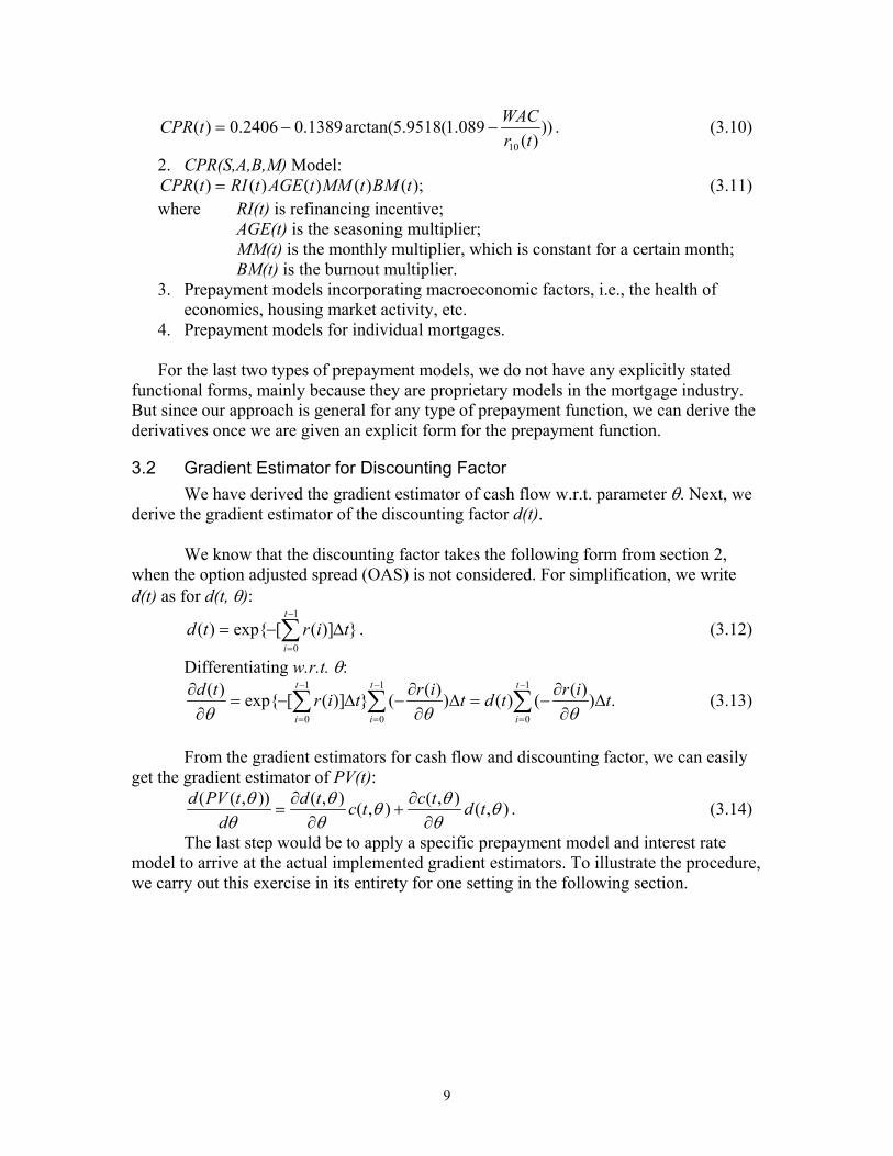
9

)))(

089.1(9518.5arctan(1389.02406.0)(10 tr

WACtCPR −−= . (3.10)

2. CPR(S,A,B,M) Model:);()()()()( tBMtMMtAGEtRItCPR = (3.11)

where RI(t) is refinancing incentive;AGE(t) is the seasoning multiplier;MM(t) is the monthly multiplier, which is constant for a certain month;BM(t) is the burnout multiplier.

3. Prepayment models incorporating macroeconomic factors, i.e., the health ofeconomics, housing market activity, etc.

4. Prepayment models for individual mortgages.

For the last two types of prepayment models, we do not have any explicitly statedfunctional forms, mainly because they are proprietary models in the mortgage industry.But since our approach is general for any type of prepayment function, we can derive thederivatives once we are given an explicit form for the prepayment function.

3.2 Gradient Estimator for Discounting FactorWe have derived the gradient estimator of cash flow w.r.t. parameter θ. Next, we

derive the gradient estimator of the discounting factor d(t).

We know that the discounting factor takes the following form from section 2,when the option adjusted spread (OAS) is not considered. For simplification, we writed(t) as for d(t, θ):

}])([exp{)(1

0tirtd

t

i∆−= ∑

−

=

. (3.12)

Differentiating w.r.t. θ:

.))(()())((}])([exp{)( 1

0

1

0

1

0tirtdtirtirtd t

i

t

i

t

i∆

∂∂

−=∆∂∂

−∆−=∂∂ ∑∑∑

−

=

−

=

−

= θθθ(3.13)

From the gradient estimators for cash flow and discounting factor, we can easilyget the gradient estimator of PV(t):

),(),(),(),()),(( θθθθ

θθ

θθ tdtctctd

dtPVd

∂∂

+∂

∂= . (3.14)

The last step would be to apply a specific prepayment model and interest ratemodel to arrive at the actual implemented gradient estimators. To illustrate the procedure,we carry out this exercise in its entirety for one setting in the following section.

10

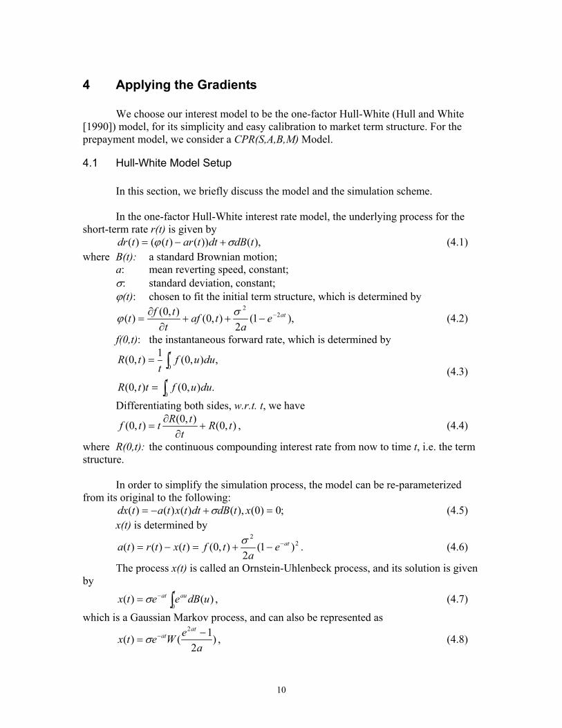
4 Applying the Gradients

We choose our interest model to be the one-factor Hull-White (Hull and White[1990]) model, for its simplicity and easy calibration to market term structure. For theprepayment model, we consider a CPR(S,A,B,M) Model.

4.1 Hull-White Model Setup

In this section, we briefly discuss the model and the simulation scheme.

In the one-factor Hull-White interest rate model, the underlying process for theshort-term rate r(t) is given by

),())()(()( tdBdttarttdr σϕ +−= (4.1)where B(t): a standard Brownian motion;

a: mean reverting speed, constant;σ: standard deviation, constant;ϕ(t): chosen to fit the initial term structure, which is determined by

),1(2

),0(),0()( 22

atea

taft

tft −−++∂

∂=

σϕ (4.2)

f(0,t): the instantaneous forward rate, which is determined by

.),0(),0(

,),0(1),0(

0

0

∫

∫=

=

t

t

duufttR

duuft

tR(4.3)

Differentiating both sides, w.r.t. t, we have

),0(),0(),0( tRt

tRttf +∂

∂= , (4.4)

where R(0,t): the continuous compounding interest rate from now to time t, i.e. the termstructure.

In order to simplify the simulation process, the model can be re-parameterizedfrom its original to the following:

;0)0(),()()()( =+−= xtdBdttxtatdx σ (4.5)x(t) is determined by

22

)1(2

),0()()()( atea

tftxtrta −−+=−=σ . (4.6)

The process x(t) is called an Ornstein-Uhlenbeck process, and its solution is givenby

∫−=t auat udBeetx0

)()( σ , (4.7)

which is a Gaussian Markov process, and can also be represented as

)2

1()(2

aeWetx

atat −

= −σ , (4.8)

11

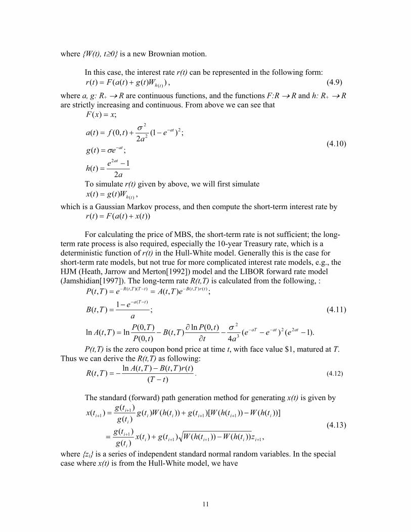
where {W(t), t≥0} is a new Brownian motion.

In this case, the interest rate r(t) can be represented in the following form:))()(()( )(thWtgtaFtr += , (4.9)

where a, g: R+ → R are continuous functions, and the functions F:R → R and h: R+ → Rare strictly increasing and continuous. From above we can see that

aeth

etg

ea

tfta

xxF

at

at

at

21)(

;)(

;)1(2

),0()(

;)(

2

22

2

−=

=

−+=

=

−

−

σ

σ

(4.10)

To simulate r(t) given by above, we will first simulate)()()( thWtgtx = ,

which is a Gaussian Markov process, and then compute the short-term interest rate by))()(()( txtaFtr +=

For calculating the price of MBS, the short-term rate is not sufficient; the long-term rate process is also required, especially the 10-year Treasury rate, which is adeterministic function of r(t) in the Hull-White model. Generally this is the case forshort-term rate models, but not true for more complicated interest rate models, e.g., theHJM (Heath, Jarrow and Merton[1992]) model and the LIBOR forward rate model(Jamshidian[1997]). The long-term rate R(t,T) is calculated from the following, :

).1()(4

),0(ln),(),0(),0(ln),(ln

;1),(

;),(),(

223

2

)(

)(),())(,(

−−−∂

∂−=

−=

==

−−

−−

−−−

atataT

tTa

trTtBtTTtR

eeeat

tPTtBtPTPTtA

aeTtB

eTtAeTtP

σ

(4.11)

P(t,T) is the zero coupon bond price at time t, with face value $1, matured at T.Thus we can derive the R(t,T) as following:

)()(),(),(ln),(

tTtrTtBTtATtR

−−

−= . (4.12)

The standard (forward) path generation method for generating x(t) is given by

,))(())(()()()()(

))](())(()[())(()()()(

)(

1111

111

1

++++

+++

+

−+=

−+=

iiiiii

i

iiiiii

ii

zthWthWtgtxtg

tg

thWthWtgthWtgtg

tgtx

(4.13)

where {zi} is a series of independent standard normal random variables. In the specialcase where x(t) is from the Hull-White model, we have

12

1

2

1 21)()( +

∆−∆−

+−

+= i

ta

ita

i za

etxetxi

i σ , (4.14)

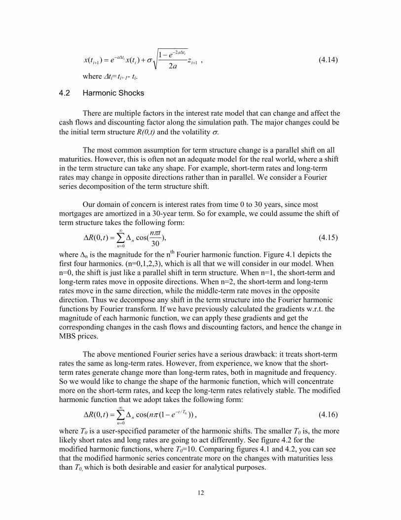
where ∆ti=ti+1- ti.

4.2 Harmonic Shocks

There are multiple factors in the interest rate model that can change and affect thecash flows and discounting factor along the simulation path. The major changes could bethe initial term structure R(0,t) and the volatility σ.

The most common assumption for term structure change is a parallel shift on allmaturities. However, this is often not an adequate model for the real world, where a shiftin the term structure can take any shape. For example, short-term rates and long-termrates may change in opposite directions rather than in parallel. We consider a Fourierseries decomposition of the term structure shift.

Our domain of concern is interest rates from time 0 to 30 years, since mostmortgages are amortized in a 30-year term. So for example, we could assume the shift ofterm structure takes the following form:

∑∞

=

∆=∆0

),30

cos(),0(n

ntntR π (4.15)

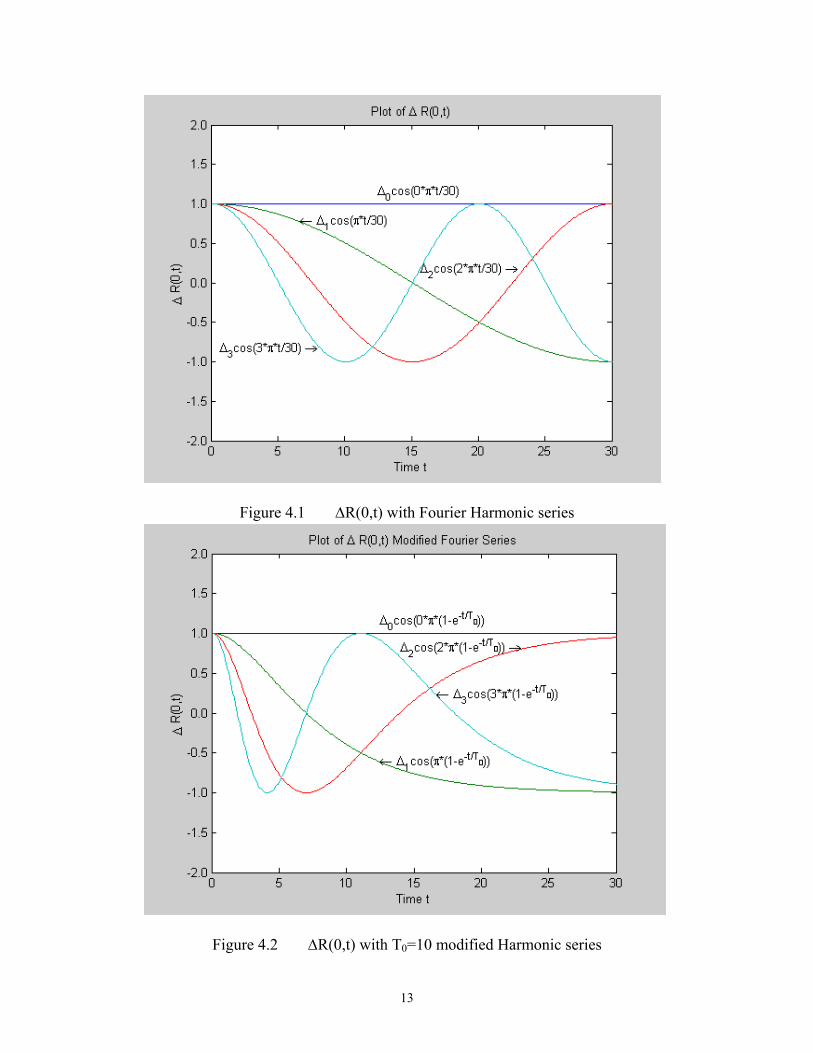
where ∆n is the magnitude for the nth Fourier harmonic function. Figure 4.1 depicts thefirst four harmonics. (n=0,1,2,3), which is all that we will consider in our model. Whenn=0, the shift is just like a parallel shift in term structure. When n=1, the short-term andlong-term rates move in opposite directions. When n=2, the short-term and long-termrates move in the same direction, while the middle-term rate moves in the oppositedirection. Thus we decompose any shift in the term structure into the Fourier harmonicfunctions by Fourier transform. If we have previously calculated the gradients w.r.t. themagnitude of each harmonic function, we can apply these gradients and get thecorresponding changes in the cash flows and discounting factors, and hence the change inMBS prices.

The above mentioned Fourier series have a serious drawback: it treats short-termrates the same as long-term rates. However, from experience, we know that the short-term rates generate change more than long-term rates, both in magnitude and frequency.So we would like to change the shape of the harmonic function, which will concentratemore on the short-term rates, and keep the long-term rates relatively stable. The modifiedharmonic function that we adopt takes the following form:

∑∞

=

−−∆=∆0

/ ))1(cos(),0( 0

n

Ttn entR π , (4.16)

where T0 is a user-specified parameter of the harmonic shifts. The smaller T0 is, the morelikely short rates and long rates are going to act differently. See figure 4.2 for themodified harmonic functions, where T0=10. Comparing figures 4.1 and 4.2, you can seethat the modified harmonic series concentrate more on the changes with maturities lessthan T0, which is both desirable and easier for analytical purposes.

13

Figure 4.1 ∆R(0,t) with Fourier Harmonic series

Figure 4.2 ∆R(0,t) with T0=10 modified Harmonic series

14

For a Fourier cosine series that has the following functional form:

∑∞

=

+=1

0 )2cos(2

)(n

n Ttna

atf π , (4.17)

the coefficients are given by a Fourier cosine transform:

∫ ==2/

0210 ,)2cos()(4 T

n ,......,,ndtT

tntfT

a π (4.18)

For our modified harmonic series, perform the following change of variables:

)1(30

'0/ Ttet −−=

and substitute into the expression of ∆R(0,t) to get

∑∞

=

∆=∆0

)60

'2cos()',0(n

ntntR π , (4.19)

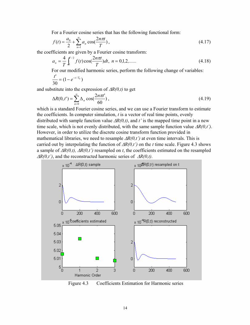
which is a standard Fourier cosine series, and we can use a Fourier transform to estimatethe coefficients. In computer simulation, t is a vector of real time points, evenlydistributed with sample function value ∆R(0,t), and t’ is the mapped time point in a newtime scale, which is not evenly distributed, with the same sample function value ∆R(0,t’).However, in order to utilize the discrete cosine transform function provided inmathematical libraries, we need to resample ∆R(0,t’) at even time intervals. This iscarried out by interpolating the function of ∆R(0,t’) on the t time scale. Figure 4.3 showsa sample of ∆R(0,t), ∆R(0,t’) resampled on t, the coefficients estimated on the resampled∆R(0,t’), and the reconstructed harmonic series of ∆R(0,t).

Figure 4.3 Coefficients Estimation for Harmonic series

15

From the chart, we can see that the reconstructed term structure matches theoriginal sample very well, which validates our method for estimating the coefficients ofthe modified harmonic series.

4.3 Derivation of Gradients w.r.t. Harmonic Functions

Our major task in this section is to derive the gradient estimator w.r.t. to specificparameters in the interest rate model and prepayment model. Specifically, for the former,we re interested in the parameters of the harmonic functions (∆n, n=0, 1, 2, 3)

First let us derive the discounting factor gradient estimator:

From (3.12), we know that in order to derive θ∂

∂ )(td , we must first derive θ∂

∂ )(ir ,

i=0,…, t-1. Let us recall that in section 4.1, we have the following simulation scheme forshort term rate r(t):

)()()( txtatr +=So

θθθ ∂∂

+∂∂

=∂∂ )()()( txtatr (4.20)

where θ∂

∂ )(ta and θ∂

∂ )(tx are determined as the following in Hull-White model:

.0)(

,),0()(

=∂∂

∂∂

=∂∂

θ

θθtx

tfta

(4.21)

We also know the relationship between f(0,t) and R(0,t) from (4.4), so θ∂

∂ ),0( tf

can be derived as:

.),0(),0(

),0(),0(),0(

),0(),0(

),0(

2

2

θθ

θθθ

θθθ

∂∂

+∂∂

∂=

∂∂

+∂∂

∂+

∂∂

∂∂

=

∂∂

+∂

∂∂

∂=

∂∂

tRt

tRt

tRt

tRtt

tRt

tRttRt

tf

(4.22)

Then we plug-in ∆n’s as θ. Considering the changes of R(0,t) which takes theform as in (4.16), we can get the derivatives of R(0,t) straight forward:

0

/

00

//

2

/

)()sin()())1(sin(),0(

)),1(cos(),0(

000

0

Ten

Tttn

Tenen

ttR

entR

TtTtTt

Tt

n−−

−

−

+−=

−−

−−=∂∂

∂

−=∆∂

∂

ππππθ

π(4.23)

We can get the derivatives of r(i):

16

))1(cos()())1(sin(),0()(0

00 /

0

// Tt

TtTt

nn

enTenenttfir −−

− −+−−=∆∂

∂=

∆∂∂ πππ (4.24)

And gradient estimator for discounting factor is also obtained, applying (3.12).

Next, we are going to derive the cash flow gradient estimator w.r.t. ∆n. From our

derivation in section 3, we know that in order to get θ∂

∂ )(tc , we need to derive θ∂

∂ )(tCPR

first. We use the second type of prepayment function, among the four described in section3. An example for this type of prepayment model is available from the sample code at theNumerix homepage http://www.numerix.com.

);()()()()( tBMtMMtAGEtRItCPR = (4.25)where

rate. mortgage prevailing ith the w correlatedhighly is which t,period of end at the observed rate,year 10 theis )(

;)0(

)1(7.03.0)(

December;in ending January, from starting 0.98], 1.23, 1.22, 1.18, 1.1, 0.98, 0.92, 0.98, 0.95, 0.74, 0.76, [0.94,)(

);30

,1min()(

)));1((430571.8arctan(14.028.0)(

10

10

trBtBtBM

tMM

ttAGE

trWACtRI

−+=

=

=

−−+−+=

From the formulas, only RI(t) and BM(t) depend on θ, when θ is not time t. Thus

we have the following formula for θ∂

∂ )(tCPR :

;)()()()()()()()()(θθθ ∂

∂+

∂∂

=∂

∂ tBMtMMtAGEtRItBMtMMtAGEtRItCPR (4.26)

where

)0(1)1(7.0)(

;)1(

)))1((430571.8(1)430(14.0)( 10

210

BtBtBM

trtrWAC

tRI

θθ

θθ

∂−∂

=∂

∂

∂−∂

−−+−+−

=∂

∂

(4.27)

(4.27)

θ∂∂ )(tB is available, when

θ∂∂ )(tc is calculated out, so the problem is reduced to

calculating θ∂

∂ )(10 tr. In the one-factor Hull-White framework, as we have discussed in

section 4.1, the long-term rate is a deterministic function of r(t), so substituting T=t+10for (4.11), we have

17

).1()(4

),0(1),0()10)(10,0(

)1()(4

),0(ln)10,(),0(ln)10,0(ln

)1()(4

),0(ln)10,(),0(

)10,0(ln)10,(ln

;11)10,(

;)10,()10,(

22)10(3

210

22)10(3

2

22)10(3

2

10)10(

)()10,()10)(10,(

−−−−

++++−=

−−−∂

∂+−−+=

−−−∂

∂+−

+=+

−=

−=+

+==+

−+−−

−+−

−+−

−−+−

+−−++−

atattaa

atatta

atatta

atta

trttBttttR

eeea

tRaettRttR

eeeat

tPttBtPtP

eeeat

tPttBtP

tPttA

ae

aettB

ettAettP

σ

σ

σ

(4.28)

Since

,10

)(1)1()(4

),0(1),0()10)(10,0(

10)()10,()10,(ln)10,()(

1022)10(

3

210

10

traeeee

atR

aettRttR

trttBttAttRtr

aatatta

a −−+−

− −−−−−

−++++−

−=

+−+−=+=

σ

(4.29)

θ∂∂ )(10 tr

takes the following form, when θ is independent of σ and t:

10

)(1),0()1()10,0()10( )(

1010

10 θθθθ

∂∂−

−∂

∂−++

∂+∂

+−−=

∂∂

−− traetR

aettRttr

aa

. (4.30)

Thus we have derived θ∂

∂ )(10 tras a function of

θ∂∂ )(tR and

θ∂∂ )(tr derived earlier.

4.4 Derivation of Gradients w.r.t. Volatility: Vega

The derivation is straightforward as in section 4.3, all we need to do is to

substitute θ with σ, instead of ∆n. In order to get σ∂

∂ )(td , we must first derive σ∂

∂ )(ir .

Following the same logic in (4.21), we can get the vega of r(t):

).2

1()1()(

so),2

1()(

,)1()(

22

2

2

22

aeWee

atr

aeWetx

ea

ta

atatat

atat

at

−+−=

∂∂

−=

∂∂

−=∂∂

−−

−

−

σσ

σ

σσ

(4.31)

And vega of d(t) would be:

.))(()()( 1

0tirtdtd t

i∆

∂∂

−=∂∂ ∑

−

= σσ(4.32)

18

Now we derive σ∂

∂ )(tc , which would require us to derive σ∂

∂ )(tCPR first, which has

the same form as in (4.27), while σ∂

∂ )(10 tr has the form of:

.10

)(1)1()(2

10

)(1)1()(2

),0()1()10,0()10(

)(

1022)10(

3

1022)10(

3

10

10

σσ

σσ

σσσ

∂∂−

+−−=

∂∂−

−−−−∂

∂−++

∂+∂

+−−=

∂∂

−−+−

−−+−

−

traeeee

a

traeeee

atR

aettRttr

aatatta

aatatta

a

(4.33)

4.5 Derivation of Second Order Gradients w.r.t. Harmonic Functions: Gamma

Another gradient that interests risk mangers is convexity, or the gamma of MBS,which is the second order derivative of price against term structure shifts. Now we derivean estimator for the gamma.

In order to calculate the partial second order derivatives (Hessian matrix),we take θ to be the vector, θ=[∆1 ∆2 ∆3 ∆4 σ]’. Differentiating (2.1), we get

.)()(')()(')()()()()(][

,)()()()()(][

02

2

2

2

02

2

2

2

2

2

00

∂∂

+∂∂

×∂∂

+∂∂

×∂∂

+∂∂

=

∂

∂=

∂∂

=∂∂

∂∂

+∂∂

=

∂

∂=

∂∂

=∂∂

∑∑

∑∑

==

==

M

t

M

t

M

t

M

t

tdtctdtctctdtctdEtPVEVEP

tdtctctdEtPVEVEP

θθθθθθθθθ

θθθθθ

(4.35)

where ]' [4321 σθ ∂∂

∆∂∂

∆∂∂

∆∂∂

∆∂∂

=∂∂ PPPPPP , and 2

2

θ∂∂ P is a 5-by-5 matrix, whose (i, j)th

element is determined by ji

Pθθ ∂∂

∂ 2

, where θI and θI are the ith and jth elements of θ,

respectively. The same notation will be used for gradients of other variables, i.e. c(t), d(t),r(t), etc.

Since we have calculated θ∂

∂ )(tc and θ∂

∂ )(td in previous sections, now the problem

is reduced to estimate 2

2 )(θ∂

∂ tc and 2

2 )(θ∂

∂ td . So we first derive the gamma for the

discounting factor d(t). Differentiating (3.12), we get

tirtdtirtdtd t

i

t

i∆×

∂∂

−×∂∂

+∆×∂∂

−×=∂∂ ∑∑

−

=

−

=

)')(()())(()()( 1

0

1

02

2

2

2

θθθθ(4.36)

19

Once we have 2

2 )(θ∂

∂ ir , the gamma of d(t) is easily calculated. Now we derive the

gamma for cash flow c(t). From (3.4), we can derive the following gamma equation:

{ }

].)()[1()(

])(][')1()(')()1([

)()](1)[()1()(

2

2

2

2

2

2

gtAtBtSMM

gtAtBtSMMtSMMtB

tSMMgtSMMtAtBtc

+−−∂

∂+

+−∂−∂

×∂

∂+

∂∂

×∂−∂

+

+−∂

−∂=

∂∂

θ

θθθθ

θθ

(4.37)

And from (3.5), we can get the gamma of B(t):

2

2

2

2

2

2 )()1()(θθθ ∂

∂−

∂−∂

=∂∂ tcgtBtB . (4.38)

Now we calculate gamma of SMM(t):

.,...,1,)(2

2

MttSMM=

∂∂

θAs we know from (3.9), we have

.)())(1(121)')()(())(1(

14411)(

2

21211

1223

2

2

θθθθ ∂∂

−+∂

∂×

∂∂

−=∂

∂ −− tCPRtCPRtCPRtCPRtCPRtSMM

(4.39)

θ∂∂ )(tCPR and 2

2 )(θ∂

∂ tCPR will be prepayment model specific.

For discounting factors, if we choose the Hull-White one factor model, we havethe following:

.5,1,)()(

;]')( )( )( )( )([)(

2

2

2

4321

≤≤

∂∂∂

=∂∂

∂∂

∆∂∂

∆∂∂

∆∂∂

∆∂∂

=∂∂

jiirir

iriririririr

ji θθθ

σθ(4.40)

From and (4.24) and (4.31), we can derive the following:

.)1()(

;0)(

;0)(

2

2

2

2

2

2

aeir

ir

ir

taii

ji

∆−−=

∂∂

=∂∆∂

∂

=∆∂∆∂

∂

σ

σ(4.41)

20

And the gamma of d(t) would be

)(/')()(

)')(()(

)')(()())(()()(

1

0

1

0

1

02

2

2

2

tdtdtd

tirtd

tirtdtirtdtd

t

i

t

i

t

i

θθ

θθ

θθθθ

∂∂

×∂∂

=

∆×∂∂

−×∂∂

=

∆×∂∂

−×∂∂

+∆×∂∂

−×=∂∂

∑

∑∑−

=

−

=

−

=

(4.42)

For cash flows, based on the equations (4.27) and (4.30) in the CPR(S, A, B, M)model, we have:

,)0(

1*)1(*7.0)(

;)1(

)))1((430571.8(15/301

)')1()1(

)()))1((430571.8(1

5/301()(

];)()(')()(

')()()()()[()()(

2

2

2

2

2

210

210

10102

10102

2

2

2

2

2

2

2

BtBtBM

trtrWAC

trtrtrWACr

tRI

tBMtRItRItBM

tBMtRItBMtRItMMtAGEtCPR

θθ

θ

θθθ

θθθ

θθθθ

∂−∂

=∂

∂

∂−∂

−−+−+

+∂−∂

×∂−∂

−−+−+∂∂

=∂

∂∂

∂+

∂∂

×∂

∂+

∂∂

×∂

∂+×

∂∂

=∂

∂

(4.43)

where we know from (4.30) that

.10

)(1

)(

0; )10,0(

;0),0(

;10

)(1),0()1(

)10,0()10(

)(

210

210

2

2

2102102

210

ji

a

ji

ji

ji

ji

a

ji

a

ji

ji

trae

tr

tR

tR

traetR

aet

tRt

tr

θθθθ

θθ

θθ

θθθθθθθθ

∂∂∂−

=∂∂

∂

=∂∂+∂

=∂∂

∂

∂∂∂−

−∂∂

∂−++

∂∂+∂

+−

−=∂∂

∂

−

−−

(4.44)

Finally, the gamma of price P given by equation (4.35) can be obtained fromequations (4.42), (4.43), and (4.44).

21

4.6 Derivation of ARM PA estimators

In this section, we derive PA estimators for ARMs. We know FRMs only havetwo sources of uncertainty:• Short-term rate r(t), which affects the discounting factor d(t), and• Long-term rate r10(t), which determines the prepayment rate CPR(t), and hence

determines the cash flow C(t).

ARMs introduce one more source of uncertainty, the coupon rate WAC(t), whichaffects both the amortization schedule and the prepayment rate CPR(t), and then affectsthe cash flow C(t). Coupon rate is determined by many factors:• The index rate. WAC resets to the index rate plus the margin periodically.• Margin. The spread between the WAC and the index rate.• Adjustment period. For fixed period (FP) ARMs, the first adjustment period is

different from subsequent adjustment period.• Period Cap/Floor. The maximum amount the WAC could increase/decrease from

previous period.• Lifetime Cap/Floor. The maximum/minimum coupon rate over the lifetime of the

mortgage.

In order to derive the PA gradient estimator of C(t) for ARM, we first need toderive the PA gradient estimator for Index(t) and WAC(t).

The most commonly used index rate is Treasury 1year rate. In the Hull-Whitemodel, it is an explicit function of short-term rate r(t) and the term structure R(0, t). Aswe have derived the function form of r10(t), we can derive the rlag(t) for any lag: (in thiscase, lag=1)

.)(1)1()(

41),0(1),0())(,0(

)(),(),(ln),()(

*22)(

3

*

lag

tra

eeeea

tRa

ettRlagtlagtR

lagtrlagttBlagttAlagttRtr

alagatatlagta

alag

lag

−−+−

− −−−−−

−−−++−

−=

+−+−=+=

(4.45)

Thus we have the PA gradient estimator of θ∂

∂ )(tIndex in following form:

lag

tra

etRa

etlagtRlagttrtIndex

alagalag

lag θθθθθ

∂∂−

−∂

∂−+−

∂+∂

+−−=

∂

∂=

∂∂

−− )(1),0()1(),0()(

)()(

**

.

(4.46)

The hard part is to get the θ∂

∂ )(tWAC from θ∂

∂ )(tIndex , because of the complicated rules to

determine WAC(t), based on all the factors mentioned above. Given WAC(t-1), Index(t),

22

Margin, Period_Cap1, Period_Floor, Life_Cap, Life_Floor, WAC(t) is determined asfollows:

≥++≥

<+<+=

+==

−=

;Margin if;Margin if

;Margin ifMargin1max

1minOtherwise,

moment; adjustmentan not is if ),1()(

CapEffective_Index(t)Cap, Effective_Index(t)FloorEffective_Floor, Effective_

CapEffective_Index(t)FloorEffective_, Index(t)WAC(t)

); Period_Cap) WAC(t-(Life_Cap,CapEffective_loor);)-Period_Fr, WAC(t-(Life_FlooFloorEffective_

ttWACtWAC

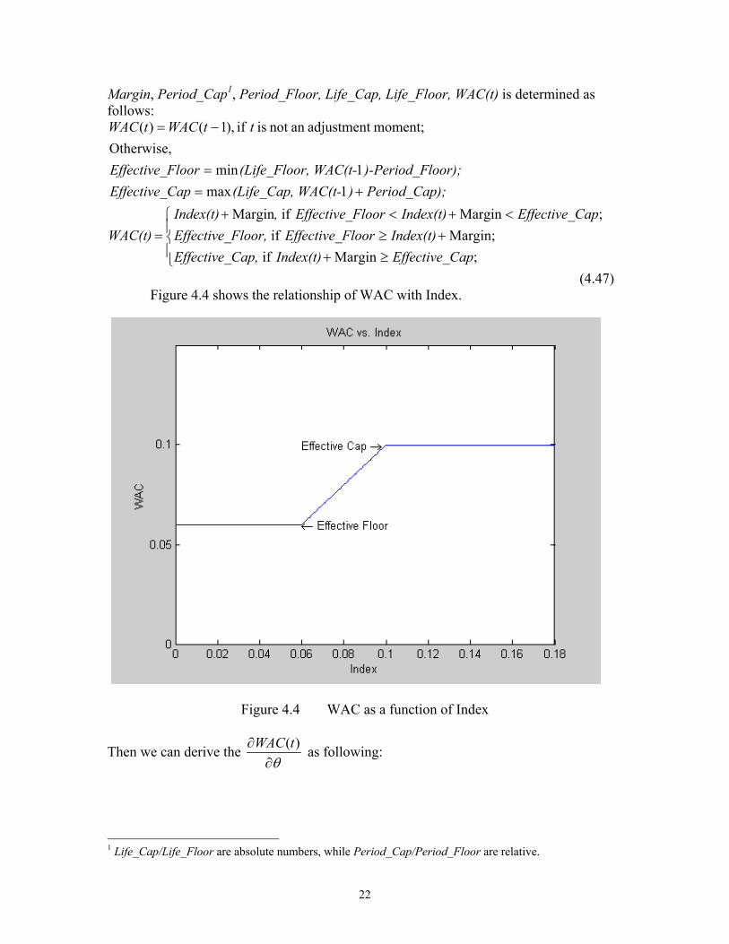
(4.47)Figure 4.4 shows the relationship of WAC with Index.

Figure 4.4 WAC as a function of Index

Then we can derive the θ∂

∂ )(tWAC as following:

1 Life_Cap/Life_Floor are absolute numbers, while Period_Cap/Period_Floor are relative.

23

=

≥+<∂

−∂

+≥>∂

−∂

<+<∂

∂

=∂

∂

+==

∂−∂

=∂

∂

false. iscondition when 0, true;iscondition when ,1

}{ where

;Margin if}__{*)1(

;Margin if}__{*)1(

;Margin if

1max1min

Otherwise,

moment; adjustmentan not is t if ,)1()(

conditionI

CapEffective_Index(t), CapLifeCapEffectiveItWAC

Index(t)FloorEffective_, FloorLifeFloorEffectiveItWAC

CapEffective_Index(t)FloorEffective_, Index(t)

WAC(t)

); Period_Cap) WAC(t-(Life_Cap,CapEffective_loor);)-Period_Fr, WAC(t-(Life_FlooFloorEffective_

tWACtWAC

θ

θ

θ

θ

θθ

(4.48)Note that the gradient is 0, when it is bounded by lifetime cap or floor, because a

perturbation would not change the WAC(t).

Next, we need to derive θ∂

∂ )(tCPR for ARM, assuming ARM borrowers have the

same prepayment behavoir as FRM borrowers (which is not necessarily true, but it doesnot affect our analysis), so we are facing the same prepayment function as FRM30 as in(4.26).

θ∂∂ )(tCPR will be affected because of the uncertainty of WAC(t).

.)0(

1)1(7.0)(

];)1()([

)))1()((430571.8(143014.0)(

;)()()()()()()()()(

102

10

BtBtBM

trtWACtrtWAC

tRI

tBMtMMtAGEtRItBMtMMtAGEtRItCPR

θθ

θθθ

θθθ

∂−∂

=∂

∂

∂−∂

−∂

∂−−+−+

=∂

∂∂

∂+

∂∂

=∂

∂

(4.49)

.)())(1(121)(

;)(11)(

1211

12

θθ ∂∂

−=∂

∂

−−=

− tCPRtCPRtSMM

tCPRtSMM(4.50)

Also C(t) will be affected by the introduced uncertainty in WAC(t):

{ })()()](1)[()1()( tSMMtgtSMMtAtBtc +−−= , (4.51)where

24

);12

)(1()(

;)12/)(1(1

12/)()(

tWACtg

tWACtWACtA tWAM

+=

+−= +−

(4.52)

And

{ }

,)()()](1[)()1(

)]()()[1()()()()](1)[()1()(

∂∂

+−∂∂

−+

+−−∂

∂++−

∂−∂

=∂∂

tSMMtgtSMMtAtB

tgtAtBtSMMtSMMtgtSMMtAtBtc

θθ

θθθ

(4.53)where

;)(121)(

;)(]

12/)(1)12/)(1())12/)(1(1(

)(144

1

)12/)(1(11

121[)(

2

θθ

θ

θ

∂∂

=∂

∂∂

++−

++−

++−

=∂∂

+−+−

+−

tWACtg

tWAC

tWACtWAMtWACtWAC

tWACtWAC

tA

tWAMtWAM

tWAM

(4.54)And the PA gradient estimator for balance B(t) is as the following:

.)(12

)1()()12

)(1()1()(

);()12

)(1)(1()(

θθθθ ∂∂−

+∂∂

−+∂−∂

=∂∂

−+−=

tWACtBtctWACtBtB

tctWACtBtB(4.55)

The PA estimator for discounting factor is unchanged, so we can get the harmonicduration and volatility duration.

25

5 Numerical Example

5.1 Specification of Numerical ExampleWe need to specify two sets of data to price the mortgage: the mortgage data and

the interest rate data, which includes the initial term structure and parameters for theinterest rate model.

We price different mortgages to examine the different impacts that a termstructure shift or change in volatility may have on different mortgage products.

The following data are fixed for all products:

Unpaid Balance/UPB =$4,000,000;WAM =360 months.

Table 5.1 shows the difference between all the products. All the ARM productshave the same subsequent adjustment period of 12 months, period cap/floor of 0.02,lifetime cap of initial WAC plus 0.06, and no lifetime floor.

Product WAC Index Adjust FirstFRM 0.07425 N/A N/A1 Year ARM 0.06425 Treasury 1 Year 12 month3/1 FP1ARM 0.07425 Treasury 1 Year 36 month5/1 FPARM 0.07425 Treasury 1 Year 60 month7/1 FPARM 0.07425 Treasury 1 Year 84 month10/1 FPARM 0.07425 Treasury 1 Year 120 month1 Year ARM2 0.07425 Treasury 10 Year 12 month

Table 5.1 Product Specification for mortgage pricing

We use the same parameters for all the different products in order to havecomparable results. Thus we set all the products to have the same coupon rate, except thefirst 1 year ARM with index of Treasury 1 year rate, which has a 100 basis points (bps)teaser rate. All the ARM products have the same characteristics, except for the AdjustFirst date, which is the feature that distinguishes these products.

Our initial term structure is the following:

f(0,t)=ln(150+12t)/100, t=0,1,…,360.

This will produce an upward-sloping curve increasing gradually from 5% to 8.7%along 30 year maturity, and R(0,t) is acquired by calculating the following: 1 FP ARM refers to Fixed Period ARM, which keep the coupon rate constant for a certain period, and thenadjust periodically, generally once a year. So All the FP ARM products are the same, except differentAdjust First date, which is the first coupon reset date.2 This ARM is not a mortgage product in the market at present, and is constructed for illustration purposeonly. The following sections will discuss why we introduce this product, and what nice properties it has.

26

);0,0()0()0,0(,),0(

),0( 0 frRt

duuftR

t

=== ∫ (5.1)

which increases from 5%, to 7.78% gradually.

Our interest rate model parameters are the following:a=0.1; σ=0.1; ∆n=0.00025, n=0,1,2,3 (used in the FD gradient and gamma

estimator calculation); ∆σ=0.00025, (used in the FD vega estimator calculation).

5.2 Comparison of PA and FD gradient estimators

In order to test whether our PA gradient estimators are accurate, and are withinthe error tolerance range, we calculate the finite difference (FD) gradient estimators at thesame time during our pricing process. This section will demonstrate the accuracy of ourPA estimators of delta, vega, and gamma for FRM, as well as the delta and gamma forARM.

Comparison of Harmonic Gradient Estimators for FRM

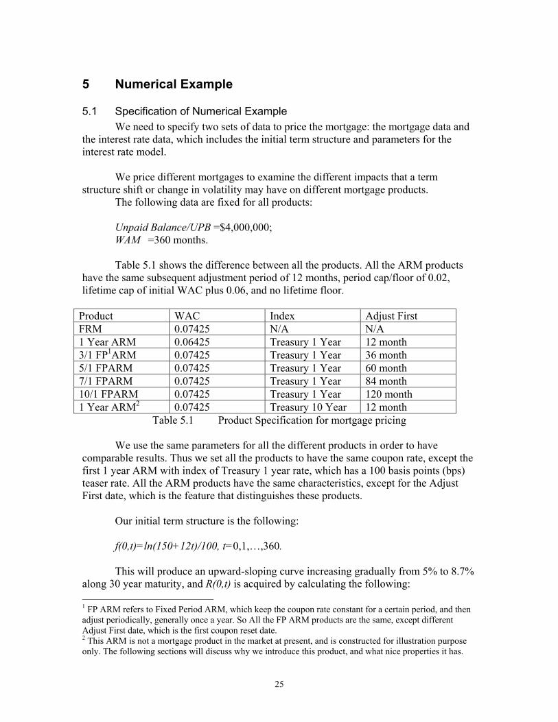
Figure 5.1 shows the FD estimator, PA estimator, their difference, and standard

deviation of their difference for n

td∆∂

∂ )( . The four curves in each chart are specified as

following, which will be the convention for the rest of the paper:Blue: Harmonic Order 1;Green: Harmonic Order 2;Red: Harmonic Order 3;Cyan: Harmonic Order 4.

We can see that although these two estimators are pretty close, there exists apattern in the difference of these two estimators. This will be explained later in the erroranalysis section.

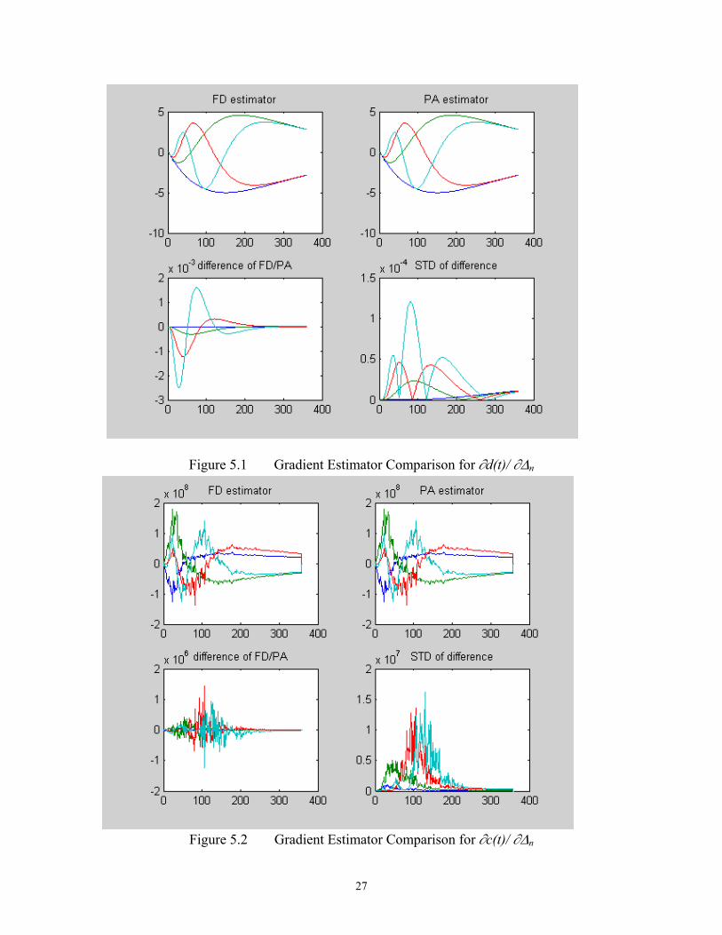
Figure 5.2 shows the gradient estimators for cash flow c(t): they are pretty close,

and the difference behaves as random noise. Based onθθ

∂∂ ),(tc and

θθ

∂∂ ),(td , we can

calculate θθ

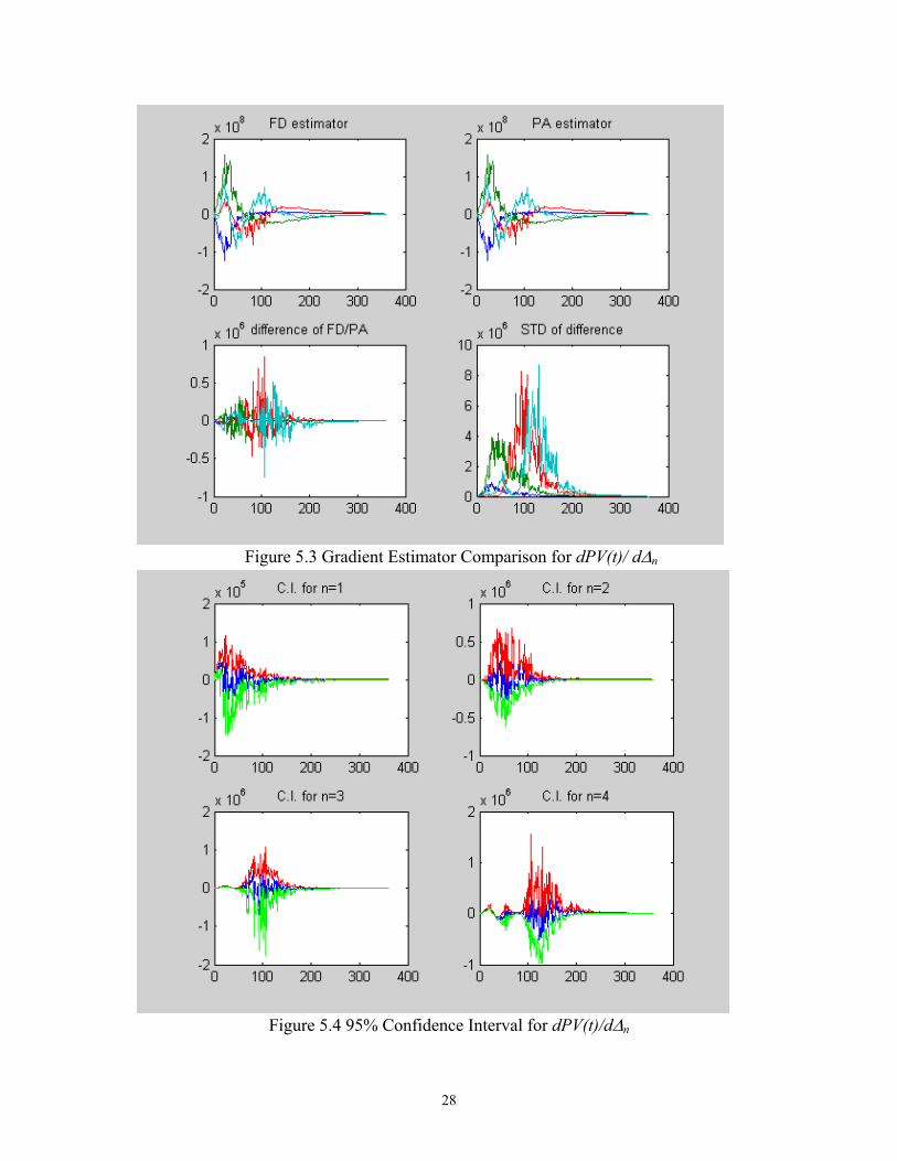
dtdPV ),( , and figure 5.3 shows us the

ndtdPV

∆)( . Figure 5.4 shows the 95%

confidence interval for ndtdPV

∆)( , and we can see that 0 is generally contained in the 95%

confidence interval.

27

Figure 5.1 Gradient Estimator Comparison for ∂d(t)/ ∂∆n

Figure 5.2 Gradient Estimator Comparison for ∂c(t)/ ∂∆n

28

Figure 5.3 Gradient Estimator Comparison for dPV(t)/ d∆n

Figure 5.4 95% Confidence Interval for dPV(t)/d∆n

29

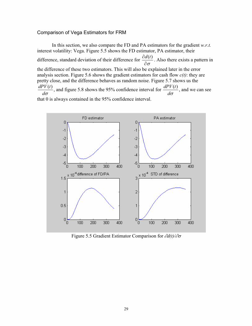
Comparison of Vega Estimators for FRM

In this section, we also compare the FD and PA estimators for the gradient w.r.t.interest volatility: Vega. Figure 5.5 shows the FD estimator, PA estimator, their

difference, standard deviation of their difference for σ∂

∂ )(td . Also there exists a pattern in

the difference of these two estimators. This will also be explained later in the erroranalysis section. Figure 5.6 shows the gradient estimators for cash flow c(t): they arepretty close, and the difference behaves as random noise. Figure 5.7 shows us the

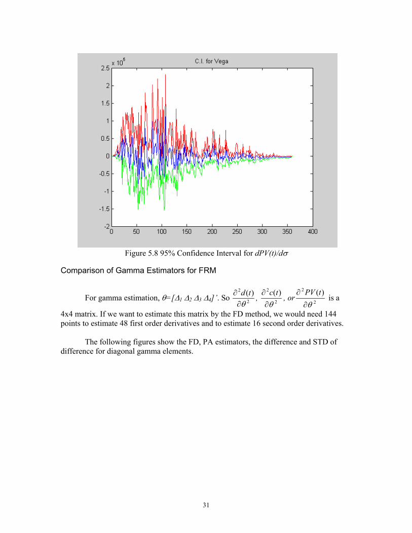
σdtdPV )( , and figure 5.8 shows the 95% confidence interval for

σdtdPV )( , and we can see

that 0 is always contained in the 95% confidence interval.

Figure 5.5 Gradient Estimator Comparison for ∂d(t)/∂σ

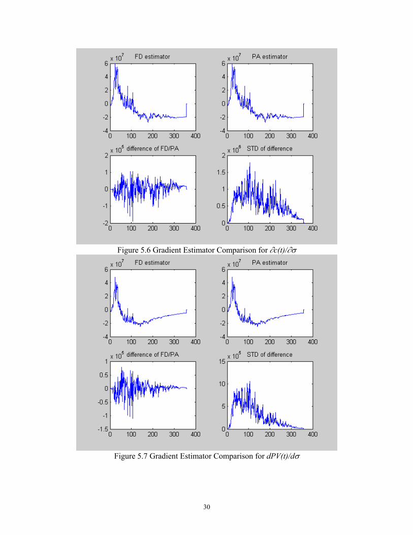
30

Figure 5.6 Gradient Estimator Comparison for ∂c(t)/∂σ

Figure 5.7 Gradient Estimator Comparison for dPV(t)/dσ

31

Figure 5.8 95% Confidence Interval for dPV(t)/dσ

Comparison of Gamma Estimators for FRM

For gamma estimation, θ=[∆1 ∆2 ∆3 ∆4]’. So 2

2 )(θ∂

∂ td , 2

2 )(θ∂

∂ tc , or2

2 )(θ∂

∂ tPV is a

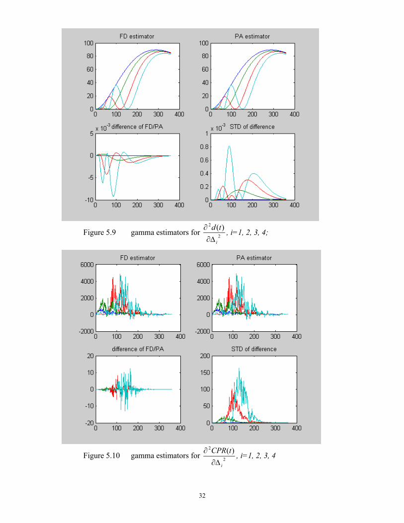
4x4 matrix. If we want to estimate this matrix by the FD method, we would need 144points to estimate 48 first order derivatives and to estimate 16 second order derivatives.

The following figures show the FD, PA estimators, the difference and STD ofdifference for diagonal gamma elements.

32

Figure 5.9 gamma estimators for 2

2 )(

i

td∆∂

∂ , i=1, 2, 3, 4;

Figure 5.10 gamma estimators for 2

2 )(

i

tCPR∆∂

∂ , i=1, 2, 3, 4

33

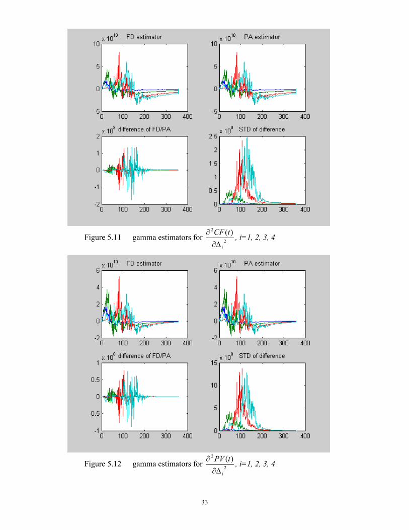
Figure 5.11 gamma estimators for 2

2 )(

i

tCF∆∂

∂ , i=1, 2, 3, 4

Figure 5.12 gamma estimators for 2

2 )(

i

tPV∆∂

∂ , i=1, 2, 3, 4

34

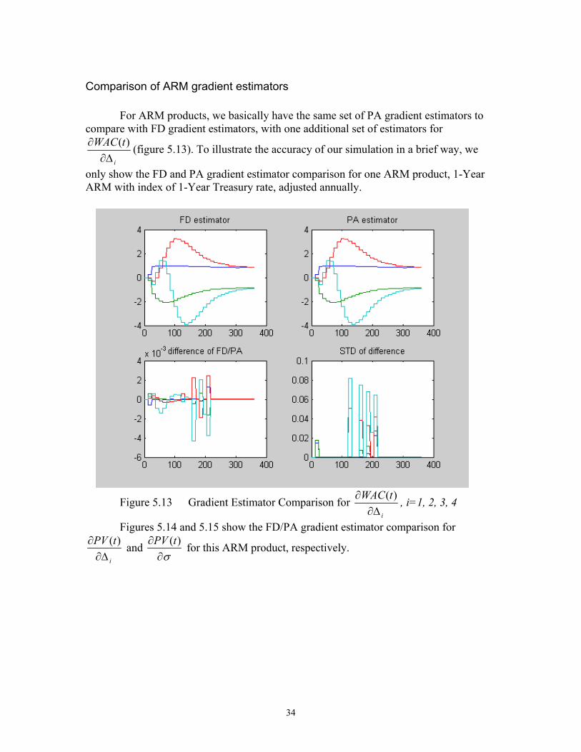
Comparison of ARM gradient estimators

For ARM products, we basically have the same set of PA gradient estimators tocompare with FD gradient estimators, with one additional set of estimators for

i

tWAC∆∂

∂ )( (figure 5.13). To illustrate the accuracy of our simulation in a brief way, we

only show the FD and PA gradient estimator comparison for one ARM product, 1-YearARM with index of 1-Year Treasury rate, adjusted annually.

Figure 5.13 Gradient Estimator Comparison for i

tWAC∆∂

∂ )( , i=1, 2, 3, 4

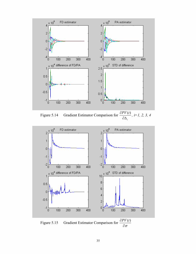
Figures 5.14 and 5.15 show the FD/PA gradient estimator comparison for

i

tPV∆∂

∂ )( and σ∂

∂ )(tPV for this ARM product, respectively.

35

Figure 5.14 Gradient Estimator Comparison for i

tPV∆∂

∂ )( , i=1, 2, 3, 4

Figure 5.15 Gradient Estimator Comparison for σ∂

∂ )(tPV

36

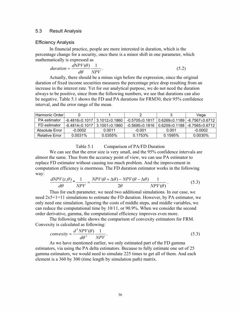
5.3 Result Analysis

Efficiency AnalysisIn financial practice, people are more interested in duration, which is the

percentage change for a security, once there is a minor shift in one parameter, whichmathematically is expressed as

NPVddNPVduration 1)(

θθ

= . (5.2)

Actually, there should be a minus sign before the expression, since the originalduration of fixed income securities measures the percentage price drop resulting from anincrease in the interest rate. Yet for our analytical purpose, we do not need the durationalways to be positive, since from the following numbers, we see that durations can alsobe negative. Table 5.1 shows the FD and PA durations for FRM30, their 95% confidenceinterval, and the error range of the mean.

Harmonic Order 0 1 2 3 VegaPA estimator -6.4816±0.1017 3.1012±0.1860 -0.5705±0.1817 0.6269±0.1189 -6.7567±0.6712FD estimator -6.4814±0.1017 3.1001±0.1860 -0.5695±0.1816 0.6259±0.1188 -6.7565±0.6712

Absolute Error -0.0002 0.0011 -0.001 0.001 -0.0002Relative Error 0.0031% 0.0355% 0.1753% 0.1595% 0.0030%

Table 5.1 Comparison of PA/FD DurationWe can see that the error size is very small, and the 95% confidence intervals are

almost the same. Thus from the accuracy point of view, we can use PA estimator toreplace FD estimator without causing too much problem. And the improvement incomputation efficiency is enormous. The FD duration estimator works in the followingway:

)(1

2)()(1*),(

θθθθθθ

θθ

NPVNPVNPV

NPVdtdNPV ∆−−∆+

= . (5.3)

Thus for each parameter, we need two additional simulations. In our case, weneed 2x5+1=11 simulations to estimate the FD duration. However, by PA estimator, weonly need one simulation. Ignoring the costs of middle steps, and middle variables, wecan reduce the computational time by 10/11, or 90.9%. When we consider the secondorder derivative, gamma, the computational efficiency improves even more.

The following table shows the comparison of convexity estimators for FRM.Convexity is calculated as following:

NPVdNPVdconvexity 1)(

2

2

θθ

= . (5.3)

As we have mentioned earlier, we only estimated part of the FD gammaestimators, via using the PA delta estimators. Because to fully estimate one set of 25gamma estimators, we would need to simulate 225 times to get all of them. And eachelement is a 360 by 300 (time length by simulation path) matrix.

37

Convexity = Gamma/Mortgage ValueMortgage Value = 4.22E+08

FD estimator 0 1 2 3 Vol0 -246.5944896 N/A N/A N/A N/A1 N/A -1871.407927 N/A N/A N/A2 N/A N/A -1854.492905 N/A N/A3 N/A N/A N/A -2000.544882 N/A

Vol N/A N/A N/A N/A -4751.605032

PA estimator0 -246.6418706 951.9319609 -646.2296558 161.8535453 919.09691791 951.9319609 -1871.360546 1251.356282 -233.9200682 -1435.4315232 -646.2296558 1251.356282 -1854.208619 1106.51252 1223.4251743 161.8535453 -233.9200682 1106.51252 -2000.92393 -715.5006989

Vol 919.1916799 -1435.407832 1223.377793 -715.4533179 -4755.158608

Harmonic Order 0 1 2 3 VolPA estimator -246.5944896 -1871.407927 -1854.492905 -2000.544882 -4751.605032FD estimator -246.6418706 -1871.360546 -1854.208619 -2000.92393 -4755.158608

Absolute Error 0.047381014 -0.047381014 -0.284286087 0.379048115 3.553576082Relative Error 0.0192% 0.0025% 0.0153% 0.0189% 0.0748%

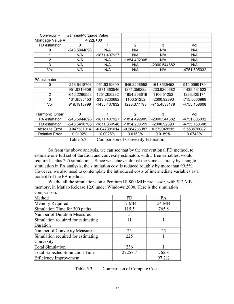
Table 5.2 Comparison of Convexity Estimators

So from the above analysis, we can see that by the conventional FD method, toestimate one full set of duration and convexity estimators with 5 free variables, wouldrequire 11 plus 225 simulations. Since we achieve almost the same accuracy by a singlesimulation in PA analysis, the simulation cost is reduced roughly by more than 99.5%.However, we also need to contemplate the introduced costs of intermediate variables as atradeoff of the PA method.

We did all the simulations on a Pentium III 800 MHz processor, with 512 MBmemory, in Matlab Release 12.0 under Windows 2000. Here is the simulationcomparison.Method FD PAMemory Required 17 MB 54 MBSimulation Time for 300 paths 115.5 765.8Number of Duration Measures 5 5Simulation required for estimatingDuration

11 1

Number of Convexity Measures 25 25Simulation required for estimatingConvexity

225 1

Total Simulation 236 1Total Expected Simulation Time 27257.7 765.8Efficiency Improvement 97.2%

Table 5.3 Comparison of Compute Costs

38

Accuracy Analysis

In order to validate the predictive power of our PA estimator, we setup a test caseto compare the predicted percentage change in the MBS price with the real percentagechange.

The test case is set up as following:

.55;3,2,1,0,55

;))1(cos(003

0

/ 0

−=∆=−=∆

−∆+= ∑=

−

ene

en ,t)R(,t)R(Perturbed_

n

n

Ttn

σ

π

(5.4)

. 004--5.0474e =

−=

∆NPV

NPVNPVPerturbed_NPVNPV

While the predicted change in NPV is calculated as following:

004--5.0414e

'21'

)('

21)'( 2

2

=

∆××∆+∆×=

∆×∂

∂×∆

+∆×

∂∂

≈∆

θθθ

θθ

θθθ

convexityduration

NPV

NPV

NPV

NPV

NPVNPV

(5.5)

where ∆θ=[∆1 ∆2 ∆3 ∆4 ∆σ].We can see that the relative error by using both duration and convexity measures

is only 0.0056%, while using duration measures only would produce a relative error of0.1403%. So this test validates the predictive power of our PA gradient estimators. In thenext section, we are going to show that PA estimator not only is more efficient than FDestimator, but also is a more accurate estimator.

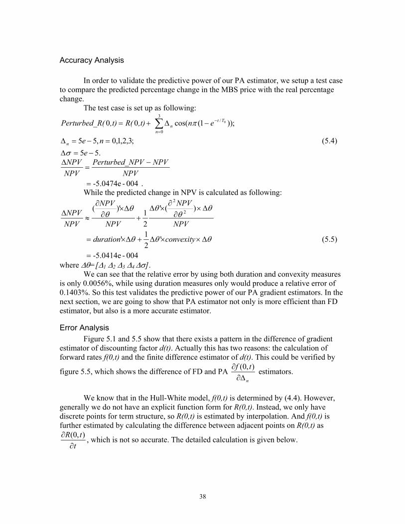
Error AnalysisFigure 5.1 and 5.5 show that there exists a pattern in the difference of gradient

estimator of discounting factor d(t). Actually this has two reasons: the calculation offorward rates f(0,t) and the finite difference estimator of d(t). This could be verified by

figure 5.5, which shows the difference of FD and PA n

tf∆∂

∂ ),0( estimators.

We know that in the Hull-White model, f(0,t) is determined by (4.4). However,generally we do not have an explicit function form for R(0,t). Instead, we only havediscrete points for term structure, so R(0,t) is estimated by interpolation. And f(0,t) isfurther estimated by calculating the difference between adjacent points on R(0,t) as

ttR

∂∂ ),0( , which is not so accurate. The detailed calculation is given below.

39

Figure 5.9 Difference of FD/PA ∂f(0, t)/ ∂∆n estimators

=∆

∆−−

<<∆

∆−−∆+

=∆−∆

=∂

∂

termmaximum theis T ,,),0(),0(

0,2

),0(),0(

0,)0,0(),0(

),0(

Ttt

tTRTR

Ttt

ttRttR

tt

RtR

ttR (5.6)

So using FD method to calculate the f(0,t) will result inaccuracy in FD estimator

of n

tr∆∂

∂ )( , and this will result inaccuracy in d(t). Also we know that d(t) takes the

following form:

}])([exp{)(1

0tirtd

t

i∆−= ∑

−

=

, and

tirtdtirtirtd t

i

t

i

t

i∆

∂∂

−=∆∂∂

−∆−=∂∂ ∑∑∑

−

=

−

=

−

=

))(()())((}])([exp{)( 1

0

1

0

1

0 θθθ. (5.7)

40

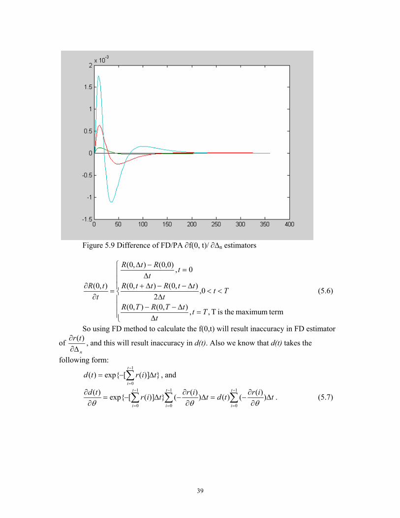
However, when we use FD method to estimate the first order derivative of e-x, theFD estimator is always greater in the absolute value, because e-x is a convex function. So

FD estimator of θ∂

∂ )(td is always biased, the bias decreases as the FD step width reduces.

The bias increases linearly, while d(t) decreases exponentially. As a result, the bias takes

the form of xe-x. Compare the difference of FD/PA σ∂

∂ )(td gradient estimators and the

figure of xe-x as follows:

For the PA method, n

tf∆∂

∂ ),0( is estimated by the following formula,

)cos(])(

)sin([ ),0(

02

0

0

0 Tttn

TtTn

Tttnttf

n ++

++−=

∆∂∂ πππ , (5.8)

which does not involve the FD estimation of t

tR∂

∂ ),0( . And θ∂

∂ )(td is directly estimated

using its analytical form of first order derivative. So the PA estimator is more accuratethan the FD estimator.

41

6 Interpretation of the Results

In this section, we briefly present the durations for various mortgage products,which show different trends for harmonic duration of different order. And we try tointerpret how the harmonic shocks of different order would affect the discounting factorsand the cash flows, and then the present value (PV) of the mortgage. Then we analyze therelationship of mortgage prepayment option and mortgage duration. Based on theseanalysis, we propose a potential new ARM product, which could reduce the duration overany of the existing mortgages, while having a less volatile index than most existingmortgages. This product would benefit both the investors who want to reduce the interestrisk, and the mortgage borrowers who want to have a fairly stable coupon rate.

6.1 Overview of the Results

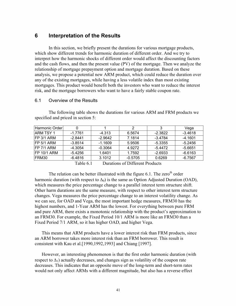
The following table shows the durations for various ARM and FRM products wespecified and priced in section 5:

Harmonic Order 0 1 2 3 VegaARM TSY 1 -1.7761 -4.313 6.5674 -2.3822 -3.4618FP 3/1 ARM -2.8441 -2.9642 7.1814 -3.4784 -4.1601FP 5/1 ARM -3.8514 -1.1609 5.9506 -5.3355 -5.2456FP 7/1 ARM -4.3054 -0.3064 4.9272 -5.4472 -5.6651FP 10/1 ARM -5.4256 1.6401 1.7592 -2.6933 -6.6163FRM30 -6.4816 3.1012 -0.5705 0.6269 -6.7567

Table 6.1 Durations of Different Products

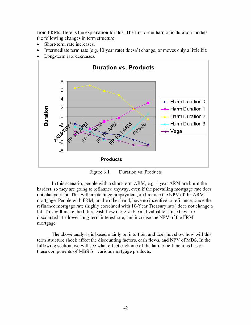
The relation can be better illustrated with the figure 6.1. The zeroth orderharmonic duration (with respect to ∆0) is the same as Option Adjusted Duration (OAD),which measures the price percentage change to a parallel interest term structure shift.Other harm durations are the same measure, with respect to other interest term structurechanges. Vega measures the price percentage change to an interest volatility change. Aswe can see, for OAD and Vega, the most important hedge measures, FRM30 has thehighest numbers, and 1-Year ARM has the lowest. For everything between pure FRMand pure ARM, there exists a monotonic relationship with the product’s approximation toan FRM30. For example, the Fixed Period 10/1 ARM is more like an FRM30 than aFixed Period 7/1 ARM, so it has higher OAD, and higher Vega.

This means that ARM products have a lower interest risk than FRM products, sincean ARM borrower takes more interest risk than an FRM borrower. This result isconsistent with Kau et al.[1990,1992,1993] and Chiang [1997].

However, an interesting phenomenon is that the first order harmonic duration (withrespect to ∆1) actually decreases, and changes sign as volatility of the coupon ratedecreases. This indicates that an opposite move of the long-term and short-term rateswould not only affect ARMs with a different magnitude, but also has a reverse effect

42

from FRMs. Here is the explanation for this. The first order harmonic duration modelsthe following changes in term structure:• Short-term rate increases;• Intermediate term rate (e.g. 10 year rate) doesn’t change, or moves only a little bit;• Long-term rate decreases.

Figure 6.1 Duration vs. Products

In this scenario, people with a short-term ARM, e.g. 1 year ARM are burnt thehardest, so they are going to refinance anyway, even if the prevailing mortgage rate doesnot change a lot. This will create huge prepayment, and reduce the NPV of the ARMmortgage. People with FRM, on the other hand, have no incentive to refinance, since therefinance mortgage rate (highly correlated with 10-Year Treasury rate) does not change alot. This will make the future cash flow more stable and valuable, since they arediscounted at a lower long-term interest rate, and increase the NPV of the FRMmortgage.

The above analysis is based mainly on intuition, and does not show how will thisterm structure shock affect the discounting factors, cash flows, and NPV of MBS. In thefollowing section, we will see what effect each one of the harmonic functions has onthese components of MBS for various mortgage products.

Duration vs. Products

-8

-6

-4

-2

0

2

4

6

8

ARM TSY 1

FP 3/1 A

RM

FP 5/1 A

RM

FP 7/1 A

RM

FP 10/1

ARM

FRM30

Products

Dur

atio

n

Harm Duration 0Harm Duration 1Harm Duration 2Harm Duration 3Vega

43

6.2 Harmonic Shock Impact

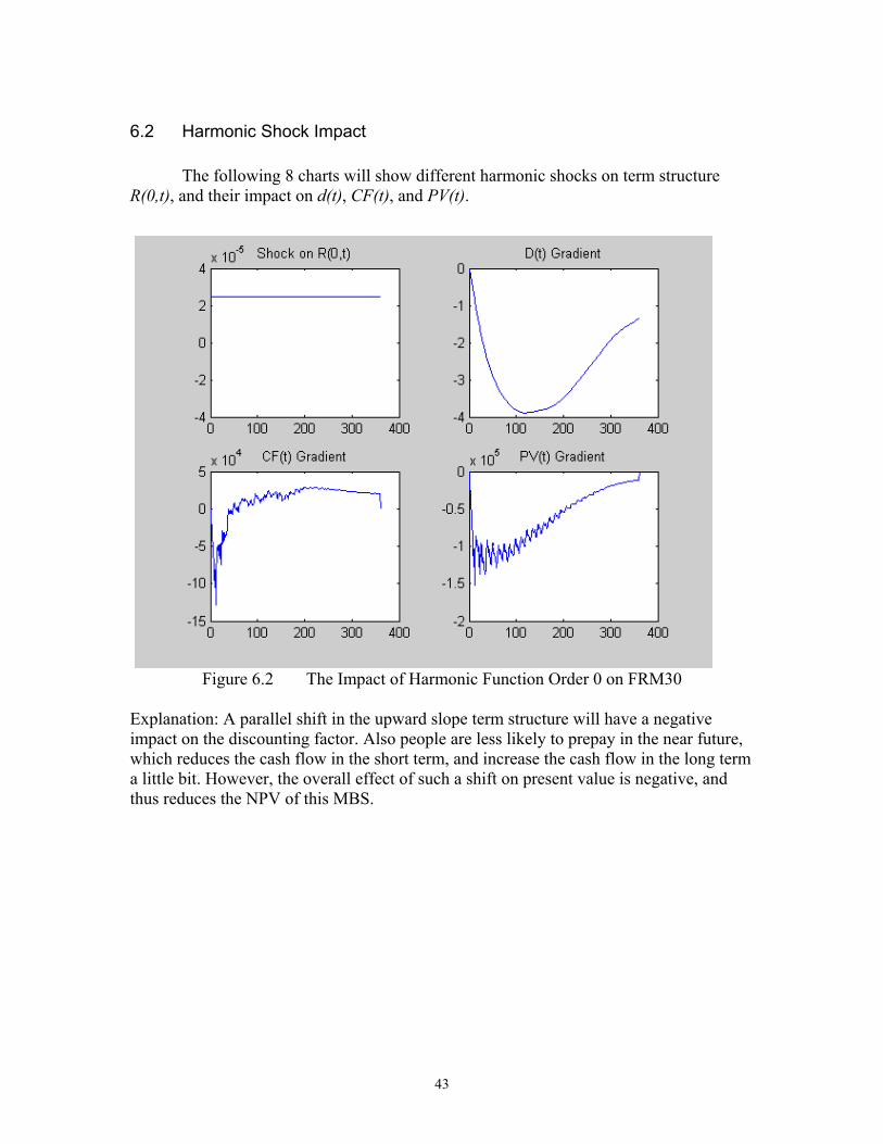
The following 8 charts will show different harmonic shocks on term structureR(0,t), and their impact on d(t), CF(t), and PV(t).

Figure 6.2 The Impact of Harmonic Function Order 0 on FRM30

Explanation: A parallel shift in the upward slope term structure will have a negativeimpact on the discounting factor. Also people are less likely to prepay in the near future,which reduces the cash flow in the short term, and increase the cash flow in the long terma little bit. However, the overall effect of such a shift on present value is negative, andthus reduces the NPV of this MBS.

44

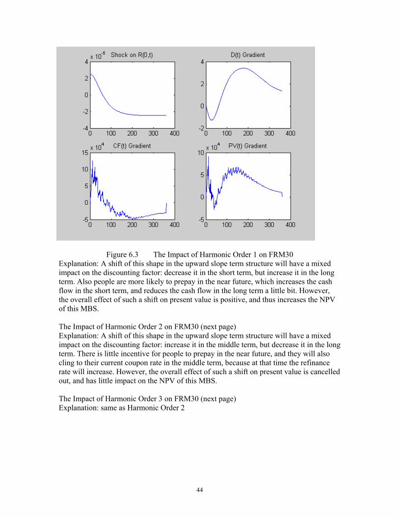
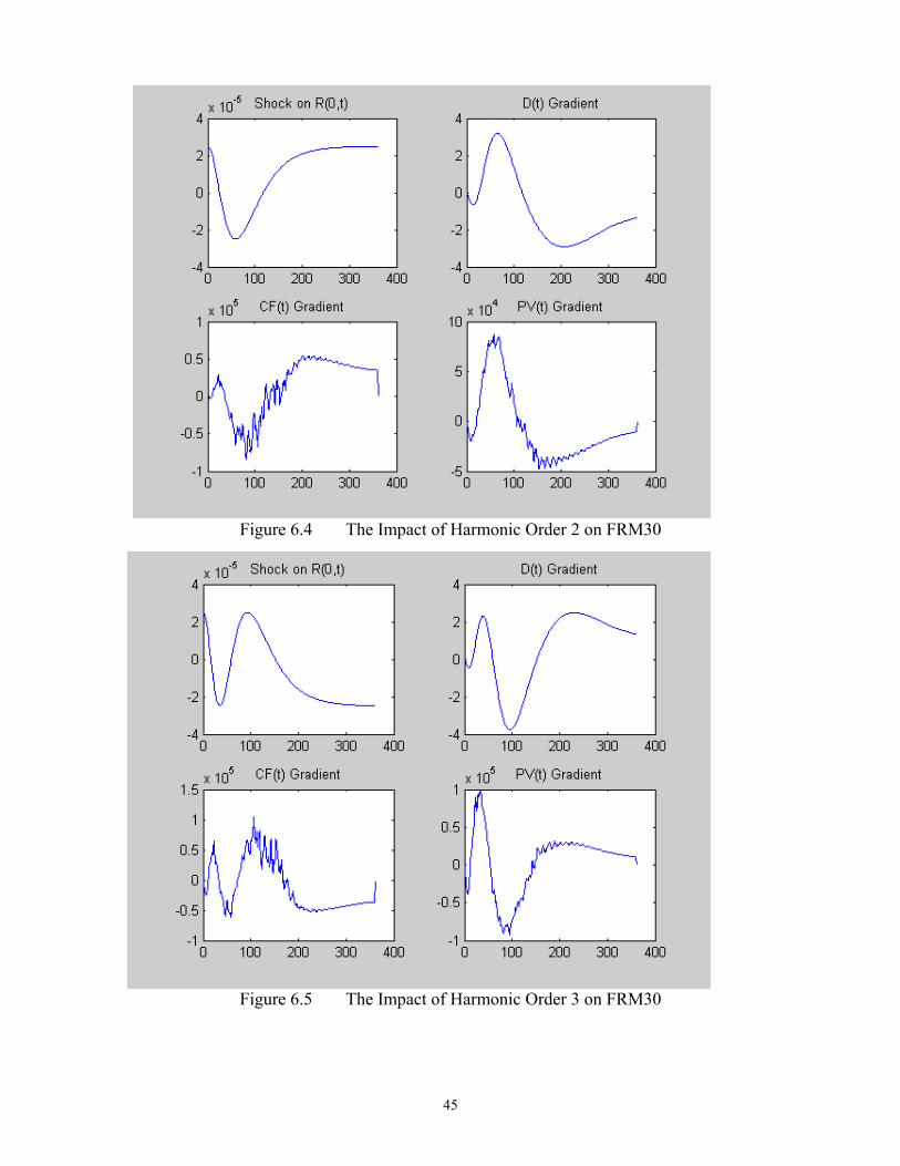
Figure 6.3 The Impact of Harmonic Order 1 on FRM30Explanation: A shift of this shape in the upward slope term structure will have a mixedimpact on the discounting factor: decrease it in the short term, but increase it in the longterm. Also people are more likely to prepay in the near future, which increases the cashflow in the short term, and reduces the cash flow in the long term a little bit. However,the overall effect of such a shift on present value is positive, and thus increases the NPVof this MBS.

The Impact of Harmonic Order 2 on FRM30 (next page)Explanation: A shift of this shape in the upward slope term structure will have a mixedimpact on the discounting factor: increase it in the middle term, but decrease it in the longterm. There is little incentive for people to prepay in the near future, and they will alsocling to their current coupon rate in the middle term, because at that time the refinancerate will increase. However, the overall effect of such a shift on present value is cancelledout, and has little impact on the NPV of this MBS.

The Impact of Harmonic Order 3 on FRM30 (next page)Explanation: same as Harmonic Order 2

45

Figure 6.4 The Impact of Harmonic Order 2 on FRM30

Figure 6.5 The Impact of Harmonic Order 3 on FRM30

46

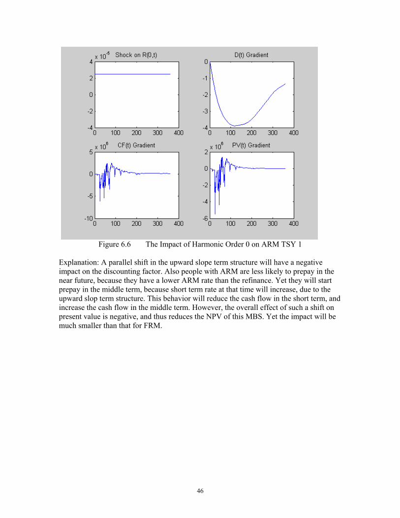
Figure 6.6 The Impact of Harmonic Order 0 on ARM TSY 1

Explanation: A parallel shift in the upward slope term structure will have a negativeimpact on the discounting factor. Also people with ARM are less likely to prepay in thenear future, because they have a lower ARM rate than the refinance. Yet they will startprepay in the middle term, because short term rate at that time will increase, due to theupward slop term structure. This behavior will reduce the cash flow in the short term, andincrease the cash flow in the middle term. However, the overall effect of such a shift onpresent value is negative, and thus reduces the NPV of this MBS. Yet the impact will bemuch smaller than that for FRM.

47

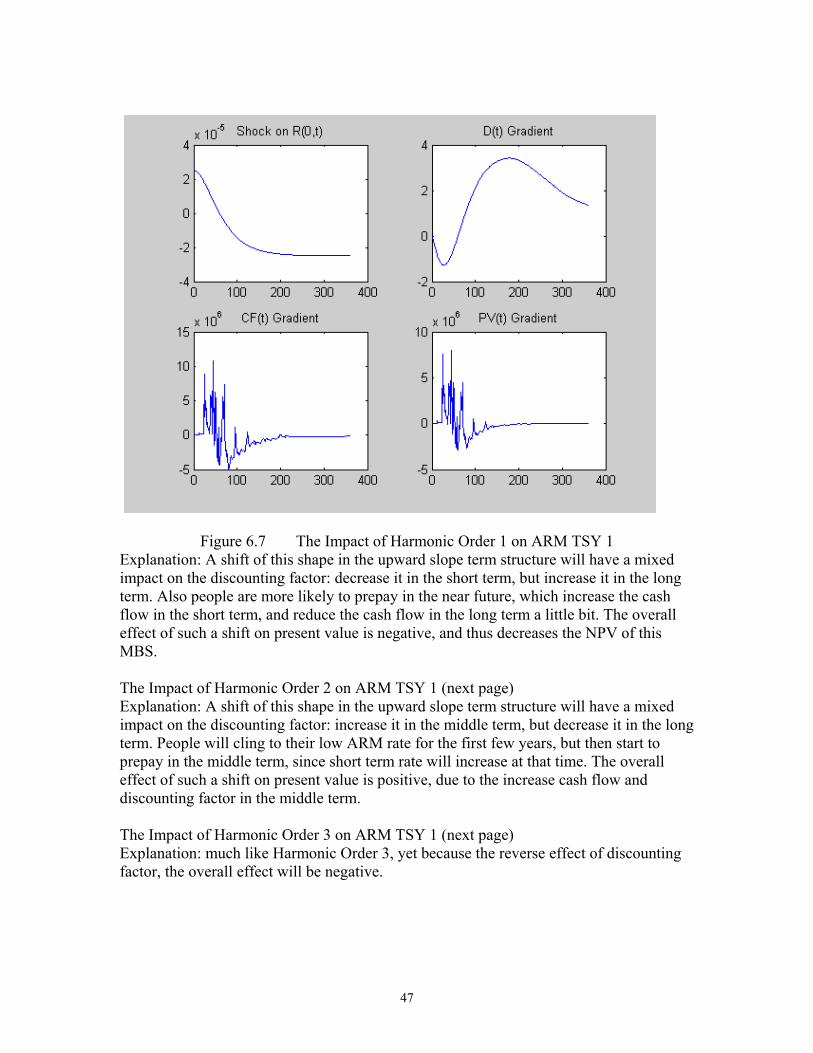
Figure 6.7 The Impact of Harmonic Order 1 on ARM TSY 1Explanation: A shift of this shape in the upward slope term structure will have a mixedimpact on the discounting factor: decrease it in the short term, but increase it in the longterm. Also people are more likely to prepay in the near future, which increase the cashflow in the short term, and reduce the cash flow in the long term a little bit. The overalleffect of such a shift on present value is negative, and thus decreases the NPV of thisMBS.

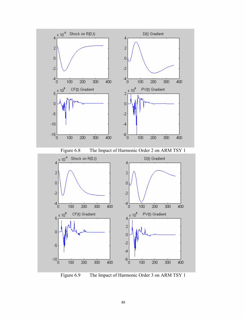
The Impact of Harmonic Order 2 on ARM TSY 1 (next page)Explanation: A shift of this shape in the upward slope term structure will have a mixedimpact on the discounting factor: increase it in the middle term, but decrease it in the longterm. People will cling to their low ARM rate for the first few years, but then start toprepay in the middle term, since short term rate will increase at that time. The overalleffect of such a shift on present value is positive, due to the increase cash flow anddiscounting factor in the middle term.

The Impact of Harmonic Order 3 on ARM TSY 1 (next page)Explanation: much like Harmonic Order 3, yet because the reverse effect of discountingfactor, the overall effect will be negative.

48

Figure 6.8 The Impact of Harmonic Order 2 on ARM TSY 1

Figure 6.9 The Impact of Harmonic Order 3 on ARM TSY 1

49

6.3 Potential New ARM Product

Duration is used to measure the interest risk of a fixed income security. Thehigher the duration is, the more interest risk that security bears. From the investor’sperspective, she will benefit if interest rates fall, and suffer if interest rates climb, if thesecurity is non-callable (no prepayment option). From the mortgage borrower’s point ofview, he will exercise his prepayment option if interest rates drop, and thus reduce thebenefit for the investor. He will be able to lock in the low mortgage rate (for FRM), incase interest rates climb, and thus hurt the investor more. However, for the ARMborrower, he benefits from the rate drop, so he does not prepay like the FRM; thus theMBS investor will also benefit. And he also pays the high coupon rate when interest ratesincrease, and the ARM MBS investor will not suffer like the FRM MBS investors. Fromthis perspective, the ARM should have a lower duration compared to FRM.

ARM borrower’s coupon rate fluctuates with the current interest rate, which iscorrelated with the prevailing mortgage rate. Because of this, she will have less incentiveto prepay when interest rate drops. So the prepayment option value for a FRM borrowerwill be larger than that of an ARM borrower. This is compatible with the market, whereFRM mortgages are sold with the highest rate (borrower pays for the valuableprepayment option), and ARM, that adjust most frequently are offered with the lowestrate.

In option theory, we know that option value generally increases as the volatility ofunderlying asset increases. However, from the above analysis, we also know that theoption value for a FRM is generally greater than for an ARM, while an ARM bears amore volatile coupon rate than a FRM. This looks like a contradiction to the option-volatility relationship. In fact, it’s not, because the underlying asset of a prepaymentoption is not its coupon rate, but the difference between the coupon rate and theprevailing mortgage rate. In most cases, the more volatile the coupon rate is, the less thedifference will be, and the less valuable the option will be. However, the borrower doesnot like the volatility, which put her at risk when interest rate jumps. The investor, on theother hand, does not like the prepayment, which reduce her investment value. It seemsthat no product can both reduce the coupon rate volatility and the prepayment option atthe same time. Is this true? We will see that we can achieve both goals in a potential newARM product.

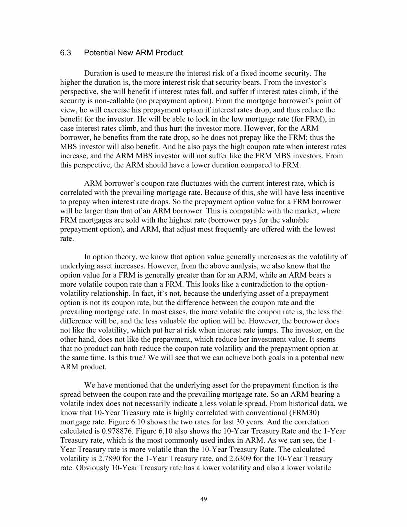
We have mentioned that the underlying asset for the prepayment function is thespread between the coupon rate and the prevailing mortgage rate. So an ARM bearing avolatile index does not necessarily indicate a less volatile spread. From historical data, weknow that 10-Year Treasury rate is highly correlated with conventional (FRM30)mortgage rate. Figure 6.10 shows the two rates for last 30 years. And the correlationcalculated is 0.978876. Figure 6.10 also shows the 10-Year Treasury Rate and the 1-YearTreasury rate, which is the most commonly used index in ARM. As we can see, the 1-Year Treasury rate is more volatile than the 10-Year Treasury Rate. The calculatedvolatility is 2.7890 for the 1-Year Treasury rate, and 2.6309 for the 10-Year Treasuryrate. Obviously 10-Year Treasury rate has a lower volatility and also a lower volatile

50

spread. The spread between conventional mortgage rate (FRM30) and 10-Year Treasuryrate and the spread between conventional mortgage rate (FRM30) and 1-Year Treasuryrate are also shown, which indicates that ARM with index of 1-Year Treasury rate has amore volatile spread.

Figure 6.10 10-Year T Rate, 1-Year T Rate, and mortgage rate

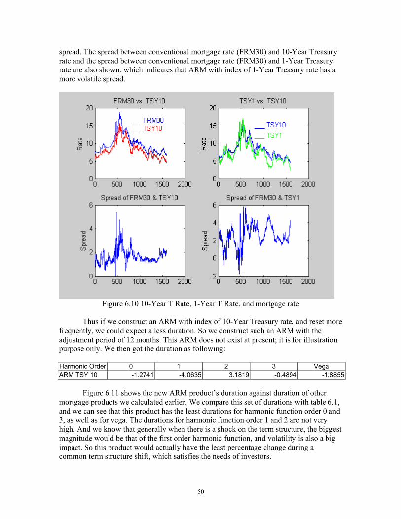
Thus if we construct an ARM with index of 10-Year Treasury rate, and reset morefrequently, we could expect a less duration. So we construct such an ARM with theadjustment period of 12 months. This ARM does not exist at present; it is for illustrationpurpose only. We then got the duration as following:

Harmonic Order 0 1 2 3 VegaARM TSY 10 -1.2741 -4.0635 3.1819 -0.4894 -1.8855

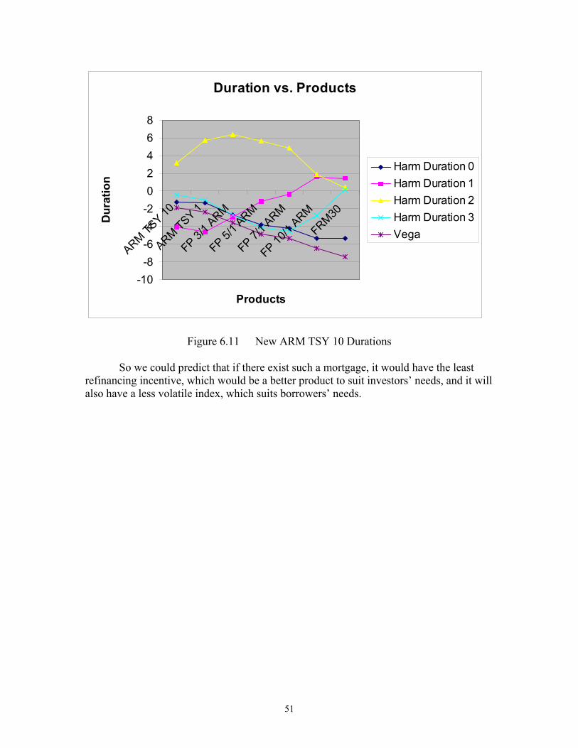
Figure 6.11 shows the new ARM product’s duration against duration of othermortgage products we calculated earlier. We compare this set of durations with table 6.1,and we can see that this product has the least durations for harmonic function order 0 and3, as well as for vega. The durations for harmonic function order 1 and 2 are not veryhigh. And we know that generally when there is a shock on the term structure, the biggestmagnitude would be that of the first order harmonic function, and volatility is also a bigimpact. So this product would actually have the least percentage change during acommon term structure shift, which satisfies the needs of investors.

51

Figure 6.11 New ARM TSY 10 Durations

So we could predict that if there exist such a mortgage, it would have the leastrefinancing incentive, which would be a better product to suit investors’ needs, and it willalso have a less volatile index, which suits borrowers’ needs.

Duration vs. Products

-10-8-6-4-202468

ARM TSY 10

ARM TSY 1

FP 3/1 A

RM

FP 5/1 A

RM

FP 7/1 A

RM

FP 10/1

ARM

FRM30

Products

Dur

atio

n

Harm Duration 0Harm Duration 1Harm Duration 2Harm Duration 3Vega

52

7 Conclusion

This paper applies perturbation analysis (PA) method to estimate MBSsensitivities. The sensitivity estimators include most interest risk measures like duration(equivalent to delta), convexity (equivalent to gamma), and vega. MBS products coveredincludes fixed rate mortgages (FRMs) and adjustable rate mortgages (ARMs).

We first derive a general framework to derive the PA estimators of MBS, withoutrestriction to MBS type, interest rate model, or prepayment model. Then we apply the PAestimator to both FRM and ARM products, in the setup of a one-factor Hull-White modeland a commonly used prepayment model. We compare the PA estimators with finitedifference (FD) estimators, and find that PA method can achieve at least the sameaccuracy as FD method, with a much lower computational cost. In the case we presented,the computational time is reduced by 95.7%, while the memory requirement increasesonly by a factor of 3, which can be handled by current computer technology with ease.Then we analyze the results of PA estimated sensitivity measures for various MBSproducts. We justify why and how different term structure shock would affect FRM andARM differently. Based these analysis, we propose a potential new ARM product whichcould benefit both the MBS investor and the mortgage borrower.

Future research includes applying this method to other MBS-like securities, sincethe PA method proposed in section 3 is a very general framework. These include otherasset-backed securities, e.g. securities backed by student loans, car loans, credit cardreceivables. It is pretty straightforward to expand this framework to those securities, sinceall that is required is to apply a specific interest rate model and prepayment model.

Another area for further research is to incorporate more complicated prepaymentand/or default models into the MBS pricing scheme. For MBS investors, the majorconcerns are price sensitivities to interest changes, which we have covered in detail.However, the MBS guarantor/insurer and issuer might have other concerns, e.g., how willthe interest rate change affect the default behavior of the mortgage borrowers? Ourframework would be able to serve this purpose as well. By applying the default modelthat same way as we apply a prepayment model, the default cash flow will take the placeof payment cash flow, so the default cost sensitivities could be easily estimated.

53

References1. Åkesson, F., and Lehoczky, J. P., Path Generation for Quasi-Monte Carlo Simulation

of Mortgage-Backed Securities, Management Science, Vol. 46, No. 9, September2000.

2. Caflisch, R.E., Morokoff, W. and Owen, A.B., Valuation of Mortgage BackedSecurities using Brownian Bridges to Reduce Effective Dimension, Journal ofComputational Finance, Vol. 1, No. 1, 1997.

3. Chiang, R., Gosnell, T. F., Heuson, A. J., Evaluating the Interest-Rate Risk ofAdjustable-Rate Mortgage Loans, Journal of Real Estate Research, Vol. 13,November 1997.

4. Fabozzi, F. J., Fixed Income Mathematics, Irwin, 1993.

5. Fu, M. C., Hu, J. Q., Sensitivity Analysis for Monte Carlo Simulation of OptionPricing, Probability in the Engineering and Information Sciences, Vol.9, No.3, 1995.

6. Fu, M. C., Madan, D.P., and Wang, T., Pricing Continuous Asian Options: AComparison of Monte Carlo and Laplace Transform Inversion Methods, Journal ofComputational Finance, Vol.2, No.2, 1999.

7. Fu, M. C., Laprise, S.B., Madan, D.B., Su, Y., and Wu, R., Pricing AmericanOptions: A Comparison of Monte Carlo Simulation Approaches, Journal ofComputational Finance, Vol.4, No.3, Spring 2001.

8. Golub, B. W., Toward a New Approach to Measuring Mortgage Duration, Chapter 25in Frank J. Fabozzi, The Handbook of Mortgage-Backed Securities, McGraw-Hill,2001.

9. Broadie, M., and Glasserman, P., Estimating Security Price Derivatives usingSimulation, Management Science, Vol. 42, 269-285, 1996.

10. Glasserman, P., Heidelberger, P., and Shahabuddin, P., Importance Sampling in theHeath-Jarrow-Morton Framework, the Journal of Derivatives, Fall 1999.

11. Glasserman, P., and Zhao, X., Fast Greeks in Forward LIBOR Model, working paper,Graduate School of Business, Columbia University, January 1999.

12. Heath, D., Jarrow, R. and Morton, A., Bond Princing and the Term Structure ofInterest Rates: A New Methodology for Contingent Claim Valuation, EconometricaVol. 60, No.1, 77–105, 1992

13. Hull, J., and White, A., Pricing interest rate derivative securities, Rev. FinancialStudies, Vol. 3, 573–592, 1990.

54

14. Jamshidian, F., Libor and swap market models and measures, Finance andStochastics, Vol.1, 293–330, 1997.

15. Kau, J. B., Keenan, D. C., The Theory of Housing and Interest Rates (in CompetitivePaper Winners), Journal of Financial and Quantitative Analysis, Vol. 15, No. 4,Proceedings of 15th Annual Conference of the Western Finance Association, June 19-21, 1980, San Diego, California. November 1980.

16. Kau, J. B., Keenan, D. C., Muller, W. J. III, Epperson, J. F., The Valuation ofAdjustable Rate Mortgage, Management Science, Vol. 36, No. 12, December, 1990.

17. Kau, J. B., Keenan, D. C., Muller, W. J. III, Epperson, J. F., A Generalized ValuationModel for Fixed-Rate Residential Mortgages, Journal of Money, Credit and Banking,Vol. 24, No. 3, August, 1992.

18. Kau, J. B., Keenan, D. C., Muller, W. J. III, Epperson, J. F., Option Theory andFloating-Rate Securities with a Comparison of Adjustable- and Fixed-RateMortgages, Journal of Business, Vol. 66, No. 4, October 1993.

19. Kpprasch, R., Understanding Duration and Convexity, Chapter 5 in Frank J. Fabozziand Irving Pollack, The Handbook of Fixed Income Securities, Dow Jones-Irwin,1987.

20. Robert A. Ott, Jr., The Duration of an Adjustable-Rate Mortgage and the Impact ofthe Index, Journal of Finance, Vol. 41, No. 4. (Sep., 1986), pp. 923-933.

21. Stanton, R., Wallace, N., Anatomy of an ARM: The Interest Rate Risk of AdjustableRate Mortgage, Journal of Real Estate Finance and Economics, Vol.19, 1999

22. Suri, R., Perturbation Analysis: The State of the Art and Research Issues Explainedvia the GI/G/1 Queue, Proceedings of the IEEE, Vol. 77, No.1, January 1989.

23. Wu, R., Fu, M. C., Optimal Exercise Policies and Simulation-based Valuation forAmerican-Asian Options," working paper, Robert H. Smith School of Business,University of Maryland, 2001.