Journal of Computational Physics 278 (2014) 378–399

Contents lists available at ScienceDirect

Journal of Computational Physics

www.elsevier.com/locate/jcp

A dispersion relation preserving optimized upwind compact

difference scheme for high accuracy flow simulations

Yogesh G. Bhumkar a,b, Tony W. H. Sheu a,c,∗, Tapan K. Sengupta d

a Center of Advanced Study in Theoretical Sciences, National Taiwan University, No. 1, Sec. 4, Roosevelt Road, Taipei, Taiwan, ROCb School of Mechanical Sciences, Indian Institute of Technology Bhubaneswar, Bhubaneswar, Odisha, Indiac Department of Engineering Science and Ocean Engineering, National Taiwan University, No. 1, Sec. 4, Roosevelt Road, Taipei, Taiwan, ROCd High Performance Computing Lab., Aerospace Engineering Department, Indian Institute of Technology Kanpur, Kanpur, U.P., India

a r t i c l e i n f o a b s t r a c t

Article history:Received 14 March 2013Received in revised form 28 June 2014Accepted 8 August 2014Available online 28 August 2014

Keywords:Compact difference schemeDRP schemeq-WavesAliasing errorFlow past an aerofoil

In this work, we have derived an optimized upwind compact difference scheme for achieving excellent spatial resolution. The derived numerical scheme adds numerical diffusion which is strictly restricted to a high wavenumber region in order to control numerical instabilities, as well as to achieve de-aliasing ability. More importantly, the derived numerical scheme has excellent dispersion relation preserving (DRP) property. The applicability of the proposed scheme in simulating real flow problems has been demonstrated by solving flow inside a lid driven cavity, a transitional flow past AG24 aerofoil and a two-dimensional decaying turbulence flow.

© 2014 Elsevier Inc. All rights reserved.

1. Introduction

Compact schemes are widely used in large eddy simulations (LES) and direct numerical simulations (DNS). These schemes have excellent spectral resolution property while numerically evaluating different derivative terms in the Navier–Stokes equations [1–10]. Compact schemes [2,7,10–12] deliver higher spectral resolution as compared to the traditional explicit discretization methods. These are implicit schemes with a compact stencil and the derivative of a function is obtained by solving a tri-diagonal [1,3,6] or a penta-diagonal [1,13] matrix equation. Although compact schemes have fewer points in the stencil, their implicit nature accounts for the contribution from large number of points inside the domain [1–3,7,12]. Thus, a higher spectral resolution is achieved even though one works on a coarser mesh. This is the principal motivation behind the wide use of compact schemes.

For accurate numerical solutions, numerical schemes must resolve all scales present in the flow. Additionally, numerical propagation speed of every individually resolved scale must be the same as the physical propagation speed of the respective scale in order to avoid dispersion error [12,14–17]. This has prompted researchers to come up with new DRP schemes [8,12,18].

The extreme form of a dispersion error has been identified as the q-waves [15,17]. These spurious waves propagate in the opposite direction, as compared to the physical direction of propagation that often leads to numerical instabilities, as well as, unphysical early bypass transition [17]. Although the amplitude of the q-waves is very small as compared to the original signal [3,17], these spurious waves are capable of creating severe numerical instabilities [3,17]. Use of higher order explicit

* Corresponding author at: Center of Advanced Study in Theoretical Sciences, National Taiwan University, No. 1, Sec. 4, Roosevelt Road, Taipei, Taiwan, ROC. Tel.: +886 2 33665746; fax: +886 2 23929885.

E-mail address: twhsheu@ntu.edu.tw (T.W.H. Sheu).

http://dx.doi.org/10.1016/j.jcp.2014.08.0400021-9991/© 2014 Elsevier Inc. All rights reserved.

Y.G. Bhumkar et al. / Journal of Computational Physics 278 (2014) 378–399 379

filters was suggested in [3–5,19] to attenuate spurious high wavenumber components responsible for numerical instabilities. In [17], generation of these spurious q-waves was attributed to insufficient mesh resolution, discontinuities present in the solution as well as in the boundary conditions, and numerical properties of the used schemes. These spurious waves are also generated due to mesh discontinuities [20]. Specifically in [3,4], the effects of curvilinear, high aspect ratio, discontinuous grids on solution accuracy have been studied for different high resolution numerical methods. Authors in [3] concluded that without the application of numerical filters, use of high-order compact schemes results in spurious oscillations and thus limits their applicability. Upwind filters have been presented in [19] to specifically control q-waves.

One should be also careful about aliasing error which originates while evaluating product terms in the transformed governing differential equations. Aliasing error occurs when the wavenumbers beyond the maximum resolvable limit are incorrectly aliased to the resolved wavenumbers [12]. As pointed out in [21,22], aliasing error is evident from an unphysical pile-up in the energy spectrum for high wavenumbers. Use of upwind schemes [22], adaptive multi-dimensional filters [10], correct zero padding [12] and skew-symmetric form of the convective terms [21] are some of the existing ways to control aliasing error.

With respect to the above discussion, we have listed below the objectives behind designing a new high accuracy scheme:

1. The scheme must have a higher spectral resolution as compared to the existing high accuracy schemes.2. The scheme must exhibit a better DRP nature across a larger wavenumber range.3. Spurious q-waves should be eliminated.4. Added numerical diffusion must be effective only near the Nyquist limit to control aliasing error and q-waves.

In the present work, we have proposed optimized stencils for the upwind compact schemes following the work in [8]. Numerical properties of the proposed schemes are analyzed using the full domain matrix global spectral analysis (GSA) technique [6,7]. These properties for the derived schemes are shown to be superior as compared to the existing high accu-racy numerical schemes. The efficiency of the proposed scheme is shown by solving the 2D and the 3D wave propagation equations on a set of different grids with significant curvature, discontinuities, large skewness with significant deviation from orthogonality. Internal and external flows governed by incompressible Navier–Stokes equation have also been simu-lated.

2. Construction of optimized upwind compact schemes

For a constant grid spacing h, the general stencil for a compact scheme for first derivative is given as,

a1u′i−1 + u′

i + a3u′i+1 = 1

h

l∑m=−l

cmui+m (1)

We have constructed various optimized upwind compact schemes by selecting different number of points on the right hand side of Eq. (1). For example, if the scheme contains three points on the right hand side of Eq. (1) then we have referred to the scheme as OP3. We have constructed a series of optimized upwind compact schemes which are identified as the OP5, OP7, OP9, OP11 and the OP13 scheme with number of points on right hand side is indicated by the numerical digits. In order to explain the methodology of optimization, we describe here the construction of the OP3 scheme. The coefficients for all the optimized schemes are separately listed in a tabular form in Appendix A (see Tables 1 and 2).

The first derivative term u′i for the OP3 scheme is approximated as,

a1∂u

∂x

∣∣∣∣i−1

+ ∂u

∂x

∣∣∣∣i+ a3

∂u

∂x

∣∣∣∣i+1

= 1

h(c−1ui−1 + c0ui + c1ui+1) (2)

The above equation contains five unknowns, namely a1, a3, c−1, c0 and c1. One needs five equations to obtain these coef-ficients. Four equations are obtained using the Taylor series expansion and by eliminating leading truncation error terms. These four equations are given as,

c−1 + c0 + c1 = 0 (3)

−c−1 + c1 − a1 − a3 = 1 (4)

a1 − a3 + c−1

2+ c1

2= 0 (5)

−a1 − a3

2− c−1 − c1

6= 0 (6)

One more algebraic equation is required to obtain all the five unknown coefficients in Eq. (2). This additional equation along with Eqs. (3)–(6) uniquely determines all the five coefficients. The exact wavenumber (K ) for Eq. (2) can be given as,

iKh(a1e−iKh + 1 + a3eiKh) = (

c−1e−iKh + c0 + c1eiKh) (7)

380 Y.G. Bhumkar et al. / Journal of Computational Physics 278 (2014) 378–399

When the first derivative term is replaced by the corresponding difference approximation, one obtains Keq as the approxi-mate wavenumber. In such case, one can write Eq. (7) as,

iKeqh(a1e−iKh + 1 + a3eiKh) = (

c−1e−iKh + c0 + c1eiKh) (8)

In general, Keq is a complex quantity with its real and imaginary parts being related to the dispersion and diffusion errors, respectively. Difference between the exact (K ) and numerically estimated wavenumber (Keq) can be minimized by closely matching them over a considerable wavenumber range.

Subsequently, the expression for the real part of Keq (denoted here by R[Keqh]) from Eq. (8) has been used to minimize numerical error. For achieving higher accuracy, R[Keqh] and Kh must be very close across the complete wavenumber range. One can construct an error function E , as defined below and optimize it by restricting it to a small value [8]. This error function has been summed over a large wavenumber range as,

E =7π8∫

0

[(Kh −R[Keqh])]2

d(Kh) (9)

In order to minimize the error function, which is summed up over the wavenumber range 0 ≤ Kh ≤ 7π8 , an additional

condition: ∂ E∂c1

= 0 is enforced. With this constraint, five unknown coefficients are uniquely determined as,

a1 = 0.4694284659989133, a3 = 0.0305715340010866,

c−1 = −1.1888569319978266, c0 = 0.8777138639956532 and c1 = 0.3111430680021733

Although the non-dimensional wavenumber Kh here varies from 0 to π , the error function E has been obtained by inte-grating over the wavenumber range 0 ≤ Kh ≤ 7π

8 for obtaining optimized coefficients with lesser computational efforts.Similarly, we have obtained the optimized coefficients for the OP5, OP7, OP9, OP11 and the OP13 schemes and listed

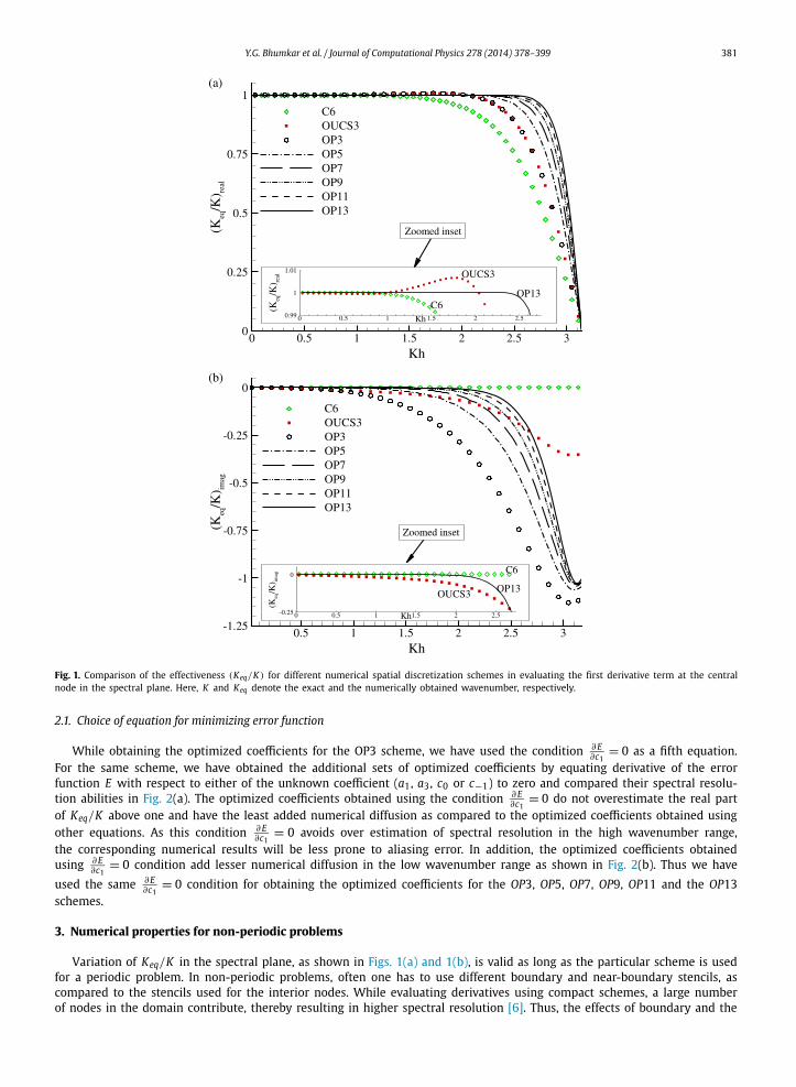
them in a tabular form in Appendix A (see Tables 1 and 2). In [3], the efficiency of the 6th order compact scheme (noted as the C6 scheme) was shown, while solving complex multi-dimensional problems involving irregular grids. In [6,7,10], the optimized upwind compact scheme OUCS3 was proposed and its efficiency while solving transitional flows was highlighted. Both the C6 scheme as well as the OUCS3 scheme have five points on the right hand side and have been previously used for high accuracy computations of complex problems. We have purposely chosen these two spatial discretization schemes to highlight the improvement in the numerical properties of the newly derived optimized upwind compact schemes. In Fig. 1(a), we have compared the spectral resolution of the different high accuracy compact schemes along with the de-veloped optimized compact schemes by plotting the real part of Keq/K with respect to the non-dimensional wavenumber (Kh). Ideally, the real part of the ratio Keq/K must be equal to one over the complete wavenumber range. However, due to the inherent implicit filtering associated with finite difference schemes, this ratio starts deviating from its ideal value even at low wavenumbers. Fig. 1(a) shows that among the indicated schemes, the scheme C6 has the least spatial resolution which is followed by the OUCS3 scheme [6]. Although the optimized scheme OP3 has only three points on the right hand side, it has the similar spatial resolution as the OUCS3 scheme, which has five points on the right hand side of the stencil. Spectral resolution increases monotonically for the derived optimized schemes as the number of points on the right hand side of Eq. (1) increases. Among all of the constructed schemes, the OP13 scheme has maximum spectral resolution. The zoomed inset at the bottom of Fig. 1(a) clearly shows that the OP13 scheme performs better as compared to the C6 and the OUCS3 schemes over the complete wavenumber range.

Fig. 1(b) shows the variation of the imaginary part of Keq/K with respect to Kh which indicates the amount of added numerical diffusion over the complete Kh range. Ideally, there should not be any added numerical diffusion. However, numerical instabilities are often experienced due to the spurious high wavenumber components [3,10]. These unphysical components need to be removed either by using explicit numerical filtering [3,19] or by adding numerical diffusion at high Kh range.

Here, we have designed the upwind compact schemes such that the added numerical diffusion is strictly restricted to the high Kh range. The negative variation of the imaginary component of Keq/K shows the added numerical diffusion. Due to the central nature of the C6 scheme, it does not add any numerical diffusion, as shown in Fig. 1(b). For the OUCS3scheme, we have used the upwind parameter as −2 [6]. The plots suggest that for the OUCS3 scheme there is a mild addition of numerical diffusion at high Kh range and an explicit filter is needed to control high Kh components responsible for numerical instabilities [10]. The present optimized compact schemes have numerical diffusion strictly restricted to the higher Kh range. The added numerical diffusion for the present schemes has a cusp-like feature with a larger numerical dissipation near the Nyquist limit. Such a cusp-like variation of the added numerical diffusion was recommended by [23,24]for LES. Out of the different proposed optimized schemes, the OP13 scheme has a better control on the added numerical diffusion. As shown in the bottom zoomed inset in Fig. 1(b), the OP13 scheme has a negligibly small diffusion up to Kh = 2.0. The numerical diffusion in case of the OP13 scheme is smaller as compared to the OUCS3 scheme up to Kh = 2.67. Thus, the present optimized upwind scheme has significantly better resolution and diffusion properties as compared to the existing high accuracy schemes.

Y.G. Bhumkar et al. / Journal of Computational Physics 278 (2014) 378–399 381

Fig. 1. Comparison of the effectiveness (Keq/K ) for different numerical spatial discretization schemes in evaluating the first derivative term at the central node in the spectral plane. Here, K and Keq denote the exact and the numerically obtained wavenumber, respectively.

2.1. Choice of equation for minimizing error function

While obtaining the optimized coefficients for the OP3 scheme, we have used the condition ∂ E∂c1

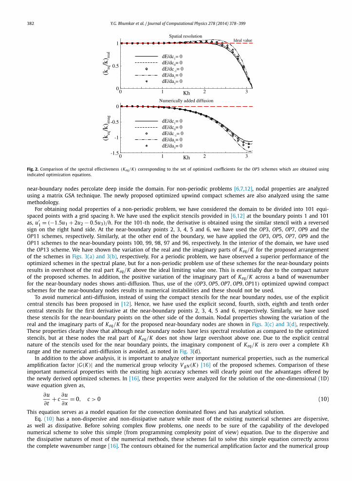
= 0 as a fifth equation. For the same scheme, we have obtained the additional sets of optimized coefficients by equating derivative of the error function E with respect to either of the unknown coefficient (a1, a3, c0 or c−1) to zero and compared their spectral resolu-tion abilities in Fig. 2(a). The optimized coefficients obtained using the condition ∂ E

∂c1= 0 do not overestimate the real part

of Keq/K above one and have the least added numerical diffusion as compared to the optimized coefficients obtained using other equations. As this condition ∂ E

∂c1= 0 avoids over estimation of spectral resolution in the high wavenumber range,

the corresponding numerical results will be less prone to aliasing error. In addition, the optimized coefficients obtained using ∂ E

∂c1= 0 condition add lesser numerical diffusion in the low wavenumber range as shown in Fig. 2(b). Thus we have

used the same ∂ E∂c1

= 0 condition for obtaining the optimized coefficients for the OP3, OP5, OP7, OP9, OP11 and the OP13schemes.

3. Numerical properties for non-periodic problems

Variation of Keq/K in the spectral plane, as shown in Figs. 1(a) and 1(b), is valid as long as the particular scheme is used for a periodic problem. In non-periodic problems, often one has to use different boundary and near-boundary stencils, as compared to the stencils used for the interior nodes. While evaluating derivatives using compact schemes, a large number of nodes in the domain contribute, thereby resulting in higher spectral resolution [6]. Thus, the effects of boundary and the

382 Y.G. Bhumkar et al. / Journal of Computational Physics 278 (2014) 378–399

Fig. 2. Comparison of the spectral effectiveness (Keq/K ) corresponding to the set of optimized coefficients for the OP3 schemes which are obtained using indicated optimization equations.

near-boundary nodes percolate deep inside the domain. For non-periodic problems [6,7,12], nodal properties are analyzed using a matrix GSA technique. The newly proposed optimized upwind compact schemes are also analyzed using the same methodology.

For obtaining nodal properties of a non-periodic problem, we have considered the domain to be divided into 101 equi-spaced points with a grid spacing h. We have used the explicit stencils provided in [6,12] at the boundary points 1 and 101as, u′

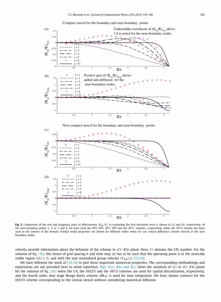
1 = (−1.5u1 + 2u2 − 0.5u3)/h. For the 101-th node, the derivative is obtained using the similar stencil with a reversed sign on the right hand side. At the near-boundary points 2, 3, 4, 5 and 6, we have used the OP3, OP5, OP7, OP9 and the OP11 schemes, respectively. Similarly, at the other end of the boundary, we have applied the OP3, OP5, OP7, OP9 and the OP11 schemes to the near-boundary points 100, 99, 98, 97 and 96, respectively. In the interior of the domain, we have used the OP13 scheme. We have shown the variation of the real and the imaginary parts of Keq/K for the proposed arrangement of the schemes in Figs. 3(a) and 3(b), respectively. For a periodic problem, we have observed a superior performance of the optimized schemes in the spectral plane, but for a non-periodic problem use of these schemes for the near-boundary points results in overshoot of the real part Keq/K above the ideal limiting value one. This is essentially due to the compact nature of the proposed schemes. In addition, the positive variation of the imaginary part of Keq/K across a band of wavenumber for the near-boundary nodes shows anti-diffusion. Thus, use of the (OP3, OP5, OP7, OP9, OP11) optimized upwind compact schemes for the near-boundary nodes results in numerical instabilities and these should not be used.

To avoid numerical anti-diffusion, instead of using the compact stencils for the near boundary nodes, use of the explicit central stencils has been proposed in [12]. Hence, we have used the explicit second, fourth, sixth, eighth and tenth order central stencils for the first derivative at the near-boundary points 2, 3, 4, 5 and 6, respectively. Similarly, we have used these stencils for the near-boundary points on the other side of the domain. Nodal properties showing the variation of the real and the imaginary parts of Keq/K for the proposed near-boundary nodes are shown in Figs. 3(c) and 3(d), respectively. These properties clearly show that although near boundary nodes have less spectral resolution as compared to the optimized stencils, but at these nodes the real part of Keq/K does not show large overshoot above one. Due to the explicit central nature of the stencils used for the near boundary points, the imaginary component of Keq/K is zero over a complete Khrange and the numerical anti-diffusion is avoided, as noted in Fig. 3(d).

In addition to the above analysis, it is important to analyze other important numerical properties, such as the numerical amplification factor |G(K )| and the numerical group velocity V gN (K ) [16] of the proposed schemes. Comparison of these important numerical properties with the existing high accuracy schemes will clearly point out the advantages offered by the newly derived optimized schemes. In [16], these properties were analyzed for the solution of the one-dimensional (1D) wave equation given as,

∂u

∂t+ c

∂u

∂x= 0, c > 0 (10)

This equation serves as a model equation for the convection dominated flows and has analytical solution.Eq. (10) has a non-dispersive and non-dissipative nature while most of the existing numerical schemes are dispersive,

as well as dissipative. Before solving complex flow problems, one needs to be sure of the capability of the developed numerical scheme to solve this simple (from programming complexity point of view) equation. Due to the dispersive and the dissipative natures of most of the numerical methods, these schemes fail to solve this simple equation correctly across the complete wavenumber range [16]. The contours obtained for the numerical amplification factor and the numerical group

Y.G. Bhumkar et al. / Journal of Computational Physics 278 (2014) 378–399 383

Fig. 3. Comparison of the real and imaginary parts of effectiveness (Keq/K ) in evaluating the first derivative term is shown in (a) and (b), respectively. At the near-boundary points 2, 3, 4, 5 and 6, we have used the OP3, OP5, OP7, OP9 and the OP11 schemes, respectively, while the OP13 scheme has been used in the interior of the domain. Similar nodal properties are shown for different nodes when we use central difference scheme stencils at the near boundary nodes.

velocity provide information about the behavior of the scheme in (Cr, Kh)-plane. Here, Cr denotes the CFL number. For the solution of Eq. (10), the choice of grid spacing h and time step �t has to be such that the operating point is in the neutrally stable region (|G| = 1) and with the unit normalized group velocity (V gN/c) [12,16].

We have followed the work of [12,16] to plot these important numerical properties. The corresponding methodology and expressions are not provided here to avoid repetition. Figs. 4(a), 4(b) and 4(c) show the variation of |G| in (Cr, Kh)-plane for the solution of Eq. (10) when the C6, the OUCS3 and the OP13 schemes are used for spatial discretization, respectively, and the fourth order, four stage Runge–Kutta scheme (RK4) is used for time integration. We have shown contours for the OUCS3 scheme corresponding to the central stencil without considering numerical diffusion.

384 Y.G. Bhumkar et al. / Journal of Computational Physics 278 (2014) 378–399

Fig. 4. Comparison of the numerical amplification factor |G j | contours for the central node corresponding to the solution of Eq. (10) when the indicated spatial discretization schemes are used with the fourth order Runge–Kutta (RK4) scheme.

Plots in Fig. 4 show that due to the central stencils of the C6 and the OUCS3 schemes, we have the desired neutrally stable region across the complete wavenumber range for a small CFL number. However due to the upwind nature of the OP13 scheme, neutrally stable region is limited to around Kh = 1 for small Cr values. This observation suggests that the C6–RK4 and the OUCS3–RK4 schemes are better than the OP13–RK4 scheme. This observation is true only if the numerical schemes offer DRP nature across the complete wavenumber range. If the numerical scheme generates q-waves and has also neutral stability, then the generated spurious components remain in the computed solution and get quickly amplified at the near-boundary nodes which are unstable in nature, thereby causing numerical instabilities [3]. As most of the central methods have spurious dispersion at higher wavenumber range, neutral stability associated with the interior nodes adds to numerical problems. If these spurious high scheme, numerical instabilities will be created at the unstable wavenumber components are not attenuated as shown for the OP13–RK4 near-boundary nodes [3]. Note that, application of extra nu-merical filters was suggested in [3,10] which in turn modifies the |G| contours in a similar way as the OP13–RK4 scheme

Y.G. Bhumkar et al. / Journal of Computational Physics 278 (2014) 378–399 385

to avoid instabilities. In Fig. 4(d), we have compared the variation of |G| for Cr = 0.1 for the above numerical schemes. This figure shows that the OP13–RK4 scheme is close to the ideal value of |G| = 1 up to Kh = 2.0 and then it attenuates higher wavenumber components. Thus, the present scheme has inbuilt essential feature of attenuating high wavenumber components. It will be also shown that the nature of the OP13–RK4 scheme to attenuate high wavenumber components helps in de-aliasing numerical solution while discussing the results of lid driven cavity flow.

Accuracy of the computed solution also depends on the ability of a numerical scheme to correctly predict the phase speed and the group velocity across complete wavenumber range. Phase speed corresponds to propagation speed of individ-ual phase, while the group velocity corresponds to propagation speed of packet of waves moving together. Since the fluid flow involves propagation of large number of spatial as well as temporal scales, a correct estimation of numerical group velocity has immense importance. The numerical and the physical group velocities must be close to each other which is usually ensured by the DRP schemes across a considerable wavenumber range [12]. In Fig. 5, we have shown the variation of the normalized numerical group velocity V gN/c in (Cr, Kh)-plane for the numerical schemes discussed in Fig. 4. We have marked a region by black color which is bounded by the contour lines corresponding to V gN/c = 0.99 and 1.01. This region has been identified as the DRP region as the group velocity is very close to the ideal value of one. The present OP13 scheme has been developed to obtain the DRP region across a larger wavenumber range. Ideally one should consider space and time discretizations together while constructing the DRP schemes [12,18]. However, higher spectral accuracy which is achieved by optimizing performance for the spatial discretization reflects in the improved DRP properties for the OP13–RK4 scheme. Since the spatio-temporal scales are related to each other through the dispersion relation, improvement in the evaluation of spatial discretization terms improves DRP properties.

While performing computations, one restricts the time step to a small value, thereby having a small CFL number to avoid numerical instabilities and to obtain maximum DRP property across the complete band of wavenumber range. In Figs. 5(a), 5(b) and 5(c), we have shown that for a small CFL number of Cr = 0.1, DRP region for the C6–RK4 scheme is limited to Kh = 1.16, while for the OUCS3–RK4 scheme it is limited to Kh = 1.76. However for the OP13–RK4 scheme, one obtains the DRP region up to Kh = 2.35 as marked in Fig. 5(c). Note that this limiting value is almost twice that is achieved for the C6–RK4 scheme and 1.35 times that is achieved for the OUCS3–RK4 scheme. A significant improvement over the already existing high accuracy schemes is therefore demonstrated.

In addition to the DRP region, we have marked a region with red color in Figs. 5(a), 5(b) and 5(c) corresponding to the negative group velocity indicating solution components in this region will not only travel with a wrong velocity but also in a wrong direction. For a chosen numerical method, the region corresponding to q-waves must be as small as possible. Figs. 5(a), 5(b) and 5(c) show that the C6–RK4 scheme has the largest q-wave region while the OP13–RK4scheme has the smallest q-wave region. The q-wave region for the C6–RK4 scheme almost starts from Kh = 2.3 while that for the OUCS3–RK4 and the OP13–RK4 schemes q-wave region nearly starts from Kh = 2.4 and Kh = 2.7, respec-tively.

Thus the present scheme has two important advantages as observed from its DRP properties, i.e, higher DRP region and significantly reduced q-wave region. We also note that due to the central nature of the C6 and the OUCS3 schemes, these schemes have neutrally stable region for small Cr value as seen in Figs. 4(a) and 4(b). For these schemes, q-waves are not only continuously created at each time step of the numerical solution but also the generated q-waves remain undamped, thereby causing a higher numerical error which is responsible for numerical instabilities. In contrast, although the OP13–RK4 scheme has a small q-wave region, the solution components corresponding to this wavenumber range are damped as seen from the |G| contours in Fig. 4(c). Good DRP property of the OP13–RK4 scheme with respect to the C6–RK4and the OUCS3–RK4 schemes has been further highlighted in Fig. 5(d).

4. Results and discussion

After analyzing numerical properties of the OP13–RK4 scheme, we now intend to use it for numerical solution of different model problems, as well as, Navier–Stokes equations. Numerical results obtained using the present scheme are compared to those obtained using the C6–RK4 scheme. Numerical results are specifically checked for the dispersion error, as well as, for the aliasing error. While carrying out numerical simulation using the C6–RK4 scheme, we have used the similar boundary and near-boundary stencils for the first and last two points in the domain as that of the OP13–RK4 scheme.

4.1. Solution of non-linear 1D advection equation

Here, we consider a non-linear pure advection equation, also known as the inviscid Burgers’ equation. The solution of Burgers’ equation displays formation of shock discontinuity with time which is usually difficult to capture correctly by using traditional low accuracy numerical schemes. In many practical applications related to high speed flows, gas dynamics, as well as combustion simulations, such discontinuities are often present in mass concentration, velocity and temperature distributions. We have considered the conservative form of Burgers’ equation given by

∂u + 1 ∂(u2) = 0 (11)

∂t 2 ∂x

386 Y.G. Bhumkar et al. / Journal of Computational Physics 278 (2014) 378–399

Fig. 5. Comparison of the numerical group velocity V gN /c contours for the central node corresponding to the solution of Eq. (10) when the indicated spatial discretization schemes are used with the fourth order Runge–Kutta (RK4) scheme. (For interpretation of the references to color in this figure legend, the reader is referred to the web version of this article.)

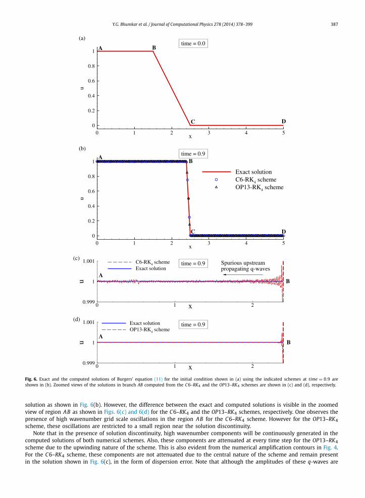
The initial condition of the solution is shown in Fig. 6(a) and is given as,

u(x) = 1.0; x ≤ 1.50

u(x) = 2.5 − x; 1.50 < x ≤ 2.50

u(x) = 0.0; x > 2.50

We have considered a domain (0 ≤ x ≤ 5) divided into 1001 equi-spaced grid points. For the present calculations, we have used a time step of 0.0005 and computed solution using the C6–RK4 and the OP13–RK4 schemes. Fig. 6(b) shows the comparison of exact solution with the solutions obtained using the OP13–RK4 and the C6–RK4 schemes. This figure shows that the solution displays a very steep shock at t = 0.9. Numerical solutions of both schemes match closely with the exact

Y.G. Bhumkar et al. / Journal of Computational Physics 278 (2014) 378–399 387

Fig. 6. Exact and the computed solutions of Burgers’ equation (11) for the initial condition shown in (a) using the indicated schemes at time = 0.9 are shown in (b). Zoomed views of the solutions in branch AB computed from the C6–RK4 and the OP13–RK4 schemes are shown in (c) and (d), respectively.

solution as shown in Fig. 6(b). However, the difference between the exact and computed solutions is visible in the zoomed view of region AB as shown in Figs. 6(c) and 6(d) for the C6–RK4 and the OP13–RK4 schemes, respectively. One observes the presence of high wavenumber grid scale oscillations in the region AB for the C6–RK4 scheme. However for the OP13–RK4scheme, these oscillations are restricted to a small region near the solution discontinuity.

Note that in the presence of solution discontinuity, high wavenumber components will be continuously generated in the computed solutions of both numerical schemes. Also, these components are attenuated at every time step for the OP13–RK4scheme due to the upwinding nature of the scheme. This is also evident from the numerical amplification contours in Fig. 4. For the C6–RK4 scheme, these components are not attenuated due to the central nature of the scheme and remain present in the solution shown in Fig. 6(c), in the form of dispersion error. Note that although the amplitudes of these q-waves are

388 Y.G. Bhumkar et al. / Journal of Computational Physics 278 (2014) 378–399

small, they are capable of triggering numerical instabilities [3]. Thus the upwind nature of the optimized schemes in the present work helps to control numerical instabilities.

4.2. Solution of 2D wave equation on irregular grid

In [25], formation of spurious q-waves was shown for the propagation of steep 2D wave packet in a domain with equi-spaced grid points. Here, we have simulated a 2D wave packet propagation on a nonuniform grid with an emphasis on studying the effects of abrupt grid discontinuities on the computed solution. The 2D wave propagation equation is given by

∂u

∂t+ cx

∂u

∂x+ c y

∂u

∂ y= 0 (12)

Consider a wave packet traveling with phase speed c = (

√c2

x + c2y ) at an angle θ with respect to the x-axis, then the

expressions for phase speeds in the x and y directions are given as cx = c cos θ and c y = c sin θ , respectively.We have constructed a domain 0 ≤ (x, y) ≤ 6 using a 551 × 551 grid. Grid has a uniform spacing of h = 0.01091 in

both the directions except in the regions 2.98798 ≤ x ≤ 3 and 2.98798 ≤ y ≤ 3, where the grid spacing is abruptly changed to h = 0.000218. As an initial condition, a 2D steep wave packet has been located at (xo = 2.6, yo = 2.6) following the equation,

u = e−500[(x−xo)2+(y−yo)2] cos[√

(x − xo)2 + (y − yo)2]

(13)

The initial solution is shown in Fig. 7(a). The grid discontinuities along the x- and the y-directions are shown by the dashed horizontal and vertical lines near x = 3 and y = 3. We consider the packet moving along a line inclined at θ = 45◦ to the x-axis with the phase speeds cx = c y = 0.1. A CFL number of Crx = 0.1 has been chosen and computations are performed with the corresponding time step. In Figs. 7(a) and 7(b), we have compared the solutions obtained using the OP13–RK4 and the C6–RK4 schemes, respectively. At t = 0.2 one does not observe q-waves. However as the packet passes through the grid discontinuities, q-waves are created for the solution of the C6–RK4 scheme as shown at t = 0.6 in Fig. 7(b). These spurious waves are attenuated for the solution of the OP13–RK4 scheme and the predicted packet retains its size and shape after passing through grid discontinuities.

Note that in many computational studies related to the high speed flows, one needs to adaptively cluster grid points near the shock region in order to correctly capture high gradient solution. Use of such discontinuous grid with a central scheme gives rise to additional spurious waves apart from those contributed by solution discontinuity [20]. Use of the highly accurate OP13–RK4 scheme resolves flow structures characterized with a large bandwidth and at the same time attenuates spurious waves, thereby controlling numerical instabilities.

4.3. Solution of 2D wave equation on wavy grid

As a next example, we have obtained a numerical solution of a 2D steep wavepacket on a smooth wavy grid with a grid size of 301 × 301. Although this grid is smooth and continuous, it has a considerably large deviation from orthogonality (±76.0631◦) and has a significant skewness. We have compared the numerical behavior of the OP13–RK4 scheme with that of the C6–RK4 scheme. The grid has been generated using the following expressions:

xi, j = (i − 1) + 5.0 × sin(0.05π( j − 1))

50

yi, j = ( j − 1) + 5.0 × sin(0.05π(i − 1))

50, 1 ≤ i ≤ 301; 1 ≤ j ≤ 301 (14)

As an initial condition, a 2D steep wave packet has been located at (xo = 2, yo = 2) following the equation given by

u = e−250[(x−xo)2+(y−yo)2] cos[√

(x − xo)2 + (y − yo)2]

(15)

The 2D convection equation (12) has been solved in a transformed (ξ, η)-plane with constant grid spacings as

∂u

∂t+ cx

(∂u

∂ξ

∂ξ

∂x+ ∂u

∂η

∂η

∂x

)+ c y

(∂u

∂ξ

∂ξ

∂ y+ ∂u

∂η

∂η

∂ y

)= 0 (16)

If one defines the Jacobian of transformation by J = (xξ yη − yξ xη)−1, then the grid metric terms are given as ξx = J yη , ηx = − J yξ , ξy = − J xη and ηy = J xξ . Substituting these into Eq. (16) we obtain

1

J

∂u

∂t+ cx

(∂u

∂ξ

∂ y

∂η− ∂u

∂η

∂ y

∂ξ

)+ c y

(−∂u

∂ξ

∂x

∂η+ ∂u

∂η

∂x

∂ξ

)= 0 (17)

Note that the above equation in the transformed plane contains several grid metrics which need to be evaluated correctly for getting a higher accuracy. Smooth nature of grid ensures continuous variation of grid metrics. However the present grid

Y.G. Bhumkar et al. / Journal of Computational Physics 278 (2014) 378–399 389

Fig. 7. Solution of a 2D wavepacket propagation over a discontinuous grid has been shown for the OP13–RK4 and the C6–RK4 schemes in (a) and (b), respectively. We have shown five different contour levels in exponential order as 0.0001, 0.001, 0.01, 0.1, 1.

has considerable deviation from orthogonality and the corresponding computations need evaluation of additional number of terms as shown in Eq. (17). These extra terms also add to the numerical error.

For this problem, we have prescribed the phase speeds as cx = 0.5 and c y = 0.5. We have computed Eq. (17) using the C6–RK4 and the OP13–RK4 schemes and the results are shown in Fig. 8. Initial condition along with the background grid is shown in the top frame of Fig. 8. Numerical solutions for the C6–RK4 and the OP13–RK4 schemes are shown in the left and right columns of Fig. 8. Once again, q-waves are seen in the solution of the C6–RK4 scheme and these waves are attenuated for the OP13–RK4 scheme. We note that although grid is smooth, Eq. (17) contains products of the solution derivative and grid metrics which contribute to the generation of high wavenumber components. One can also observe that even for a simple wave propagation problem on a wavy grid solved using the C6–RK4 scheme, a large part of the domain is filled up with spurious waves. Thus, computations performed on a smooth grid are also affected by q-waves and numerical schemes must be carefully designed to control undesirable effects of q-waves. The bottom frame of Fig. 8 compares the spectral contents of the solution on the mid-plane at t = 2 obtained using the C6–RK4 and the OP13–RK4 schemes. One can observe

390 Y.G. Bhumkar et al. / Journal of Computational Physics 278 (2014) 378–399

Fig. 8. Initial condition of a wavepacket and the background wavy grid are shown in the top frame. Solutions of a 2D wavepacket propagation have been shown for the C6–RK4 and the OP13–RK4 schemes in the left and the right columns, respectively. We have shown six different contour levels in exponential order as 0.00001, 0.0001, 0.001, 0.01, 0.1, 1. Bottom frame shows the comparison of FFT of the signal at t = 2 on the mid-plane for the C6–RK4 and the OP13–RK4 schemes.

from the FFT that the spectral contents of the C6–RK4 and the OP13–RK4 schemes differ only in the high wavenumber range due to aliasing. This is the same wavenumber range which corresponds to the region where the added numerical diffusion is significant in the OP13–RK4 scheme. Thus, use of the optimized upwind OP13–RK4 scheme attenuates the solution in the high wavenumber range only, where numerical diffusion is absolutely necessary.

4.4. Solution of 3D wave equation on wavy grid

Similar to the previous example involving a wavy grid, we have obtained the numerical solution of a 3D steep wavepacket on a smoothly varying wavy grid. Grid size for this problem is kept as 81 × 81 × 81. Once again we have obtained solutions using the C6–RK4 and the OP13–RK4 schemes. The following expressions have been used to construct 3D grid:

Y.G. Bhumkar et al. / Journal of Computational Physics 278 (2014) 378–399 391

xi, j,k = �x((i − 1) + sin(0.5π) sin

(π( j − 1)�y

)sin

(π(k − 1)�z

))yi, j,k = �y

(( j − 1) + sin(0.5π) sin

(π(i − 1)�x

)sin

(π(k − 1)�z

))zi, j,k = �z

((k − 1) + sin(0.5π) sin

(π( j − 1)�y

)sin

(π(i − 1)�x

)), 1 ≤ i ≤ 81; 1 ≤ j ≤ 81; 1 ≤ k ≤ 81 (18)

We have used �x = �y = �z = 0.05. A 3D steep wave packet has been located initially at (xo = yo = z0 = 1.9512)

following the equation,

u = e−64[(x−xo)2+(y−yo)2+(z−zo)2] cos[5√

(x − xo)2 + (y − yo)2 + (z − zo)2]

(19)

Similar to the 2D case in Eq. (12), the 3D convection equation can be written as,

∂u

∂t+ cx

∂u

∂x+ c y

∂u

∂ y+ cz

∂u

∂z= 0 (20)

Here cx , c y and cz are the phase speeds in their respective directions. For the present computations, we have considered motion of a wavepacket along the x-axis by specifying phase speeds cx = 1 and c y = cz = 0. Eq. (20) in the physical plane (x, y, z) needs to be transformed to the computational plane (ξ, η, ζ ) with the constant grid spacings similar to Eq. (17). However while performing 3D computations, one should be careful about the issues of freestream preservation and metric cancellation [3,26,27]. While performing the present 3D computation, we have followed the suggestions in [3,4] of using the same high accuracy scheme to obtain both the flux, as well as, the grid derivative terms for higher accuracy. In these references for an effective metric cancellation, it was recommended to compute the metric relations in the following forms:

ξ̂x = yηzζ − yζ zη = (yηz)ζ − (yζ z)η

η̂x = yζ zξ − yξ zζ = (yζ z)ξ − (yξ z)ζ

ζ̂x = yξ zη − yηzξ = (yξ z)η − (yηz)ξ (21)

Similarly, one can obtain the remaining grid metric terms. The initial condition and three sections of the used wavy grids are shown in the top left and the top right frames of Fig. 9. Solutions obtained using the C6–RK4 scheme at different instants again display trailing spurious q-waves in the form of 3D disturbances. Such disturbances are in attenuated form for the solution of the OP13–RK4 scheme and are not visible in the solution, as seen in the solutions obtained from the C6–RK4scheme.

4.5. Navier–Stokes simulation of lid driven cavity flow

We have obtained the solution of a 2D lid driven cavity flow for a Reynolds number (Re = 7500) to solve one of the existing benchmark problems. Another motivation behind solving this problem is to demonstrate the de-aliasing property of the OP13 scheme. In [22], it was shown that due to the discontinuous boundary velocity condition near the top right corner of the lid driven cavity, high wavenumber components are generated continuously resulting in some unphysical pile-up of high wavenumber components. This is an indication of aliasing error in the computed solution. The cusp-like feature present in the variation of imaginary part of Keq/K as noted in Fig. 1(b) for the OP13 scheme should help to control the aliasing error significantly.

Lid driven cavity problem has been widely studied by different researchers in [8,22,28]. Here, we have considered the fluid motion inside a square cavity closed by four solid walls. The top surface moves with a uniform speed while the remaining three surfaces are stationary. We have solved the Navier–Stokes equations formulated in the streamfunction and vorticity formulation in the transformed (ξ, η)-plane given as [12],

∂

∂ξ

[h22

h11

∂ψ

∂ξ

]+ ∂

∂η

[h11

h22

∂ψ

∂η

]= −h11h22ω (22)

h11h22∂ω

∂t+ h22u

∂ω

∂ξ+ h11 v

∂ω

∂η= 1

Re

[∂

∂ξ

(h22

h11

∂ω

∂ξ

)+ ∂

∂η

(h11

h22

∂ω

∂η

)](23)

where the parameters h11 =√

(x2ξ + y2

ξ ) and h22 =√

(x2η + y2

η) are grid scale factors.

For the time integration of Eq. (23), RK4 scheme has been used while for the spatial discretization of convective terms in Eq. (23), we have used the OP13 scheme. Dissipation terms in Eqs. (22), (23) are discretized using the CD2 scheme. We have used a uniformly spaced 351 × 351 grid for the present computations and compared our results with the results in [28]. Figs. 10(a) and 10(b) show the streamfunction contours obtained in [28] and the present numerical study, respectively, for a Reynolds number of Re = 7500. The central vortex (primary vortex) and the bottom left (BL1) and the bottom right (BR1) vortices match well with the results of [28].

We have also computed the lid driven cavity flow using the C6–RK4 scheme for the spatial discretization of convective terms in Eq. (23) for Re = 7500. Fast Fourier transform (FFT) of the vorticity data on the top surface has been obtained at t = 100, as indicated in Fig. 10(c). As discussed earlier, discontinuity in the velocity boundary condition near the top

392 Y.G. Bhumkar et al. / Journal of Computational Physics 278 (2014) 378–399

Fig. 9. Initial condition of a wavepacket and sections of 3D wavy grid are shown in top left and right frames, respectively. Solution of a 3D wavepacket propagation over a wavy grid has been shown for the C6–RK4 and the OP13–RK4 schemes in the left and right columns. We have shown iso-surface level of 0.0001 in the above figures.

right corner triggers high wavenumber components, which cause the unphysical pile-up of solution, shown in Fig. 10(c). In contrast, the upwinding of the OP13 scheme does not allow occurrence of pile-up of high wavenumber components and controls aliasing error effectively, as shown in Fig. 10(d).

4.6. Transitional flows past AG24 aerofoil

We have simulated a physically unstable 2D flow past AG24 aerofoil, for which the experimental results are provided in [29]. We have once again used the OP13 scheme for the non-linear convection terms in Eq. (23). The vorticity transport equation is time-advanced using the RK4 time integration scheme, while the diffusion terms are discretized in self-adjoint form using the second order central difference (CD2) scheme. We have constructed a truly orthogonal grid [12] with 528 ×

Y.G. Bhumkar et al. / Journal of Computational Physics 278 (2014) 378–399 393

Fig. 10. Comparison of the streamfunction contours for Re = 7500 between the results (a) in [28] and (b) the present work. FFT of the vorticity data along the top surface is shown for the C6 and the OP13 schemes in (c) and (d), respectively, at the indicated instants. Result for the C6 scheme shows unphysical rise in the tail amplitude.

289 grid points and the outer boundary of the domain is around 10 chord distance from the surface of aerofoil. At the inlet, we have provided a potential flow boundary condition while at the outlet a convective boundary condition on the radial component of velocity (also called the Sommerfeld boundary condition) is applied. On the aerofoil surface we have prescribed no-slip condition. Domain decomposition methodology has been used to solve this problem while performing parallel computing [30]. We have used MPI FORTRAN-90 compiler with four processors to demonstrate the ability of the proposed scheme in the parallel computing environment.

394 Y.G. Bhumkar et al. / Journal of Computational Physics 278 (2014) 378–399

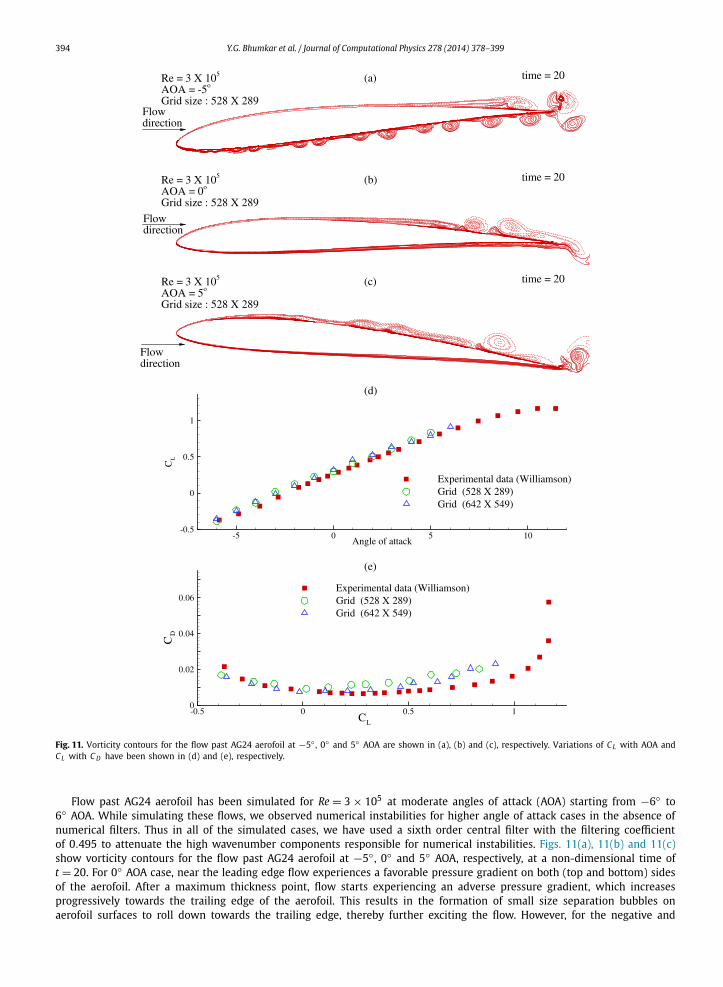
Fig. 11. Vorticity contours for the flow past AG24 aerofoil at −5◦ , 0◦ and 5◦ AOA are shown in (a), (b) and (c), respectively. Variations of CL with AOA and CL with C D have been shown in (d) and (e), respectively.

Flow past AG24 aerofoil has been simulated for Re = 3 × 105 at moderate angles of attack (AOA) starting from −6◦ to 6◦ AOA. While simulating these flows, we observed numerical instabilities for higher angle of attack cases in the absence of numerical filters. Thus in all of the simulated cases, we have used a sixth order central filter with the filtering coefficient of 0.495 to attenuate the high wavenumber components responsible for numerical instabilities. Figs. 11(a), 11(b) and 11(c)show vorticity contours for the flow past AG24 aerofoil at −5◦ , 0◦ and 5◦ AOA, respectively, at a non-dimensional time of t = 20. For 0◦ AOA case, near the leading edge flow experiences a favorable pressure gradient on both (top and bottom) sides of the aerofoil. After a maximum thickness point, flow starts experiencing an adverse pressure gradient, which increases progressively towards the trailing edge of the aerofoil. This results in the formation of small size separation bubbles on aerofoil surfaces to roll down towards the trailing edge, thereby further exciting the flow. However, for the negative and

Y.G. Bhumkar et al. / Journal of Computational Physics 278 (2014) 378–399 395

Fig. 12. Vorticity contours for 2D decaying turbulence inside a square container are shown in frames (a) to (f). Here a no-slip condition at the domain boundaries has been prescribed. FFT of 1D energy spectra at t = 10 and t = 15 are shown in frames (g) and (h), respectively.

positive AOA cases, flow on either side of the aerofoil experiences higher adverse pressure gradient, as shown in Figs. 11(a) and 11(c).

Numerical method used to simulate such physically unstable flows must be very accurate to resolve all the important scales [31]. We have obtained the mean lift and drag coefficients using a coarse 528 × 289 grid, as well as, a comparatively finer mesh with 642 × 549 grid points. The variation of the numerically evaluated mean lift coefficients for different AOAs match closely with the results in [29], as shown in Fig. 11(d). In addition, the variations of the mean lift and drag coefficients also show good match between the computed and the experimental results. Thus, the use of high accuracy DRP schemes helps to solve the transitional flows accurately.

4.7. Decaying two-dimensional (2D) turbulence inside a square container

Two-dimensional decaying turbulence inside a square container is one of the important research problems studied in [32–34]. During various flow development stages, different small scale vortical structures interact with each other and form large coherent vortical structures by the inverse energy cascade process [32,33]. Numerical simulations reported in [32,33]have prescribed the initial flow field which contains a large number of equal-sized Gaussian vortices and obtained the numerical solution with either no-slip or periodic boundary conditions prescribed on the domain boundaries. Numerical simulation of this flow problem must resolve a large band of spatio-temporal scales. We have investigated this problem in order to demonstrate the capabilities of the proposed numerical scheme.

396 Y.G. Bhumkar et al. / Journal of Computational Physics 278 (2014) 378–399

Fig. 13. Vorticity contours for the 2D decaying turbulence inside a square container are shown in frames (a) to (f). Here a periodic boundary condition at the domain boundaries has been prescribed. FFT of 1D energy spectra at t = 10 and t = 13 are shown in frames (g) and (h), respectively.

We have considered a square domain with (−1 ≤ x, y ≤ 1). This domain has been discretized into 1024 equi-spaced grid points in each direction. Two-dimensional Navier–Stokes equation in streamfunction-vorticity formulation as given by Eqs. (22) and (23) are solved to obtain the decaying 2D turbulence flow field. We have considered 100 nearly equal sized Gaussian vortices which are randomly located inside the domain as an initial condition. Vortices have a dimensionless radius of 0.05 and the magnitude of peak amplitude of individual vortices is kept close to 100. Positive and negative circulations have been assigned to have the equal number of vortices.

We have obtained the numerical solution corresponding to either a periodic boundary condition or a no-slip boundary condition at the domain boundaries. Prescription of no-slip condition implies flow evolution inside a square cavity with solid boundary walls, while a periodic boundary condition excludes the effects of wall boundary layer on flow development. Presence of multiple small scale vortices induces velocity field throughout the domain. In order to ensure a no-slip condi-tion at domain boundaries, a smoothing function has been used on the vorticity distribution [33]. Numerical solutions are obtained using a time step of 0.001 corresponding to a Reynolds number of Re = 10 000 which is based on the RMS velocity value of the initial flow field and the half width of the container [33].

In Figs. 12(a) to 12(f), different stages of 2D decaying turbulence flow field in the presence of solid domain boundaries have been shown. At t = 5, one observes formation of medium sized dipoles due to a rapid self organization or merging process among the similar-sign vortices. In addition, the formation of wall boundary layer due to prescription of no-slip condition at the domain boundaries results in steepening of the vorticity gradients. There is a strong interaction between the individual vortex close to the domain boundaries and the boundary layer formed on the container walls. This strong interaction causes an ejection of thin vorticity filaments in the flow field. Due to interaction between the wall boundary

Y.G. Bhumkar et al. / Journal of Computational Physics 278 (2014) 378–399 397

Fig. 14. Variation of the mean enstrophy inside a square domain and on the domain boundaries has been shown with respect to time in frames (a) and (b), respectively.

layer and vortices close to solid walls, vorticity does not decay monotonically for this case as seen from the maximum and minimum vorticity value variations with time. As time progresses, process of merging of different vortical structures continues to form larger coherent vortical structures with their dimensions comparable to that of the domain. Figs. 12(g) and 12(h) show one-dimensional energy spectra at time t = 10 and 15, respectively. It is obtained by finding the mean of one-dimensional energy spectrum corresponding to the velocity distribution on the lines y = 0 and x = 0. Figures show the K −3 spectrum which is an indication of 2D turbulence as suggested in [32–34].

Prescription of a periodic boundary condition on the domain boundaries avoids complex interaction between the wall boundary layer and neighboring vortices as shown in Figs. 13(a) to 13(f). In this case, absence of no-slip condition avoids the injection of additional small scale vortical structures inside the domain as compared to the results in Figs. 12(a) to 12(f). In the periodic boundary case, vortical structures rapidly merge to form a large coherent vortical structure as seen from the vorticity contours at t = 50. Energy spectrum during initial flow evolution stage shows the K −3 spectrum as observed in Figs. 13(g) and 13(h). Further, in Fig. 14(a) we have shown the variation of mean enstrophy inside complete domain with time. For the periodic boundary case, the mean enstrophy inside a complete domain decays continuously and rapidly as compared to the no-slip boundary case for which there is a continuous interaction between the boundary layer formed on the domain boundaries [35]. During such strong interactions, mean enstrophy inside the domain increases, as also evident from Fig. 14(b), which shows the variation of mean enstrophy on the domain boundaries with time.

5. Summary and conclusions

In this work, we have developed high accuracy DRP scheme suitable for simulating complex flows. Excellent numerical properties and correct use of boundary stencils for non-periodic problems have been explained with the help of Figs. 1–3. Superiority of the newly developed scheme is also explained with the help of important numerical properties such as the numerical amplification factor and the numerical group velocity contours in Figs. 4 and 5, respectively. For the developed OP13–RK4 scheme, low dispersive nature and significantly less contribution to spurious q-waves are observed in the model 2D and 3D wavepacket problems shown in Figs. 6–9. The OP13 scheme has been found better for solving problems contain-ing steep gradients used in the solution and in the evaluation of grid metric terms. De-aliasing nature of the OP13 scheme has been explained in Fig. 10 with a lid driven cavity example and the proposed scheme has been used successfully to simulate transitional flow over AG24 aerofoil at different angles of attack as shown in Fig. 11. In addition, the proposed scheme successfully resolved K −3 spectrum for the 2D decaying turbulence problem as shown in Figs. 12 and 13.

Thus the proposed optimized upwind compact scheme (OP13) has excellent resolution and significantly improves DRP property across a wide wavenumber region. The upwind nature of the scheme adds numerical diffusion only in the high wavenumber range near the Nyquist limit. The scheme has significantly less contribution to spurious q-waves and these

398 Y.G. Bhumkar et al. / Journal of Computational Physics 278 (2014) 378–399

spurious high wavenumber components are further attenuated. De-aliasing and DRP nature of the proposed scheme makes it suitable for high accuracy simulation of flows.

Acknowledgement

This work was supported by the National Science Council of the Republic of China under Grant 101R891002.

Appendix A

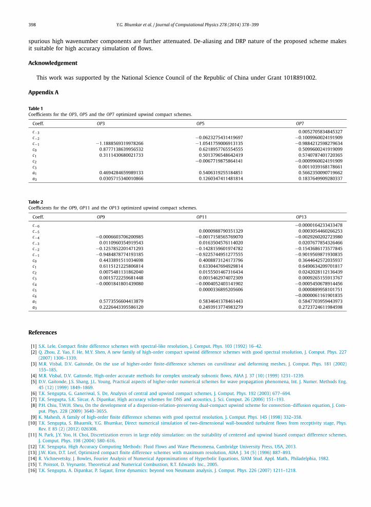
Table 1Coefficients for the OP3, OP5 and the OP7 optimized upwind compact schemes.

Coeff. OP3 OP5 OP7

c−3 0.0052705834845327c−2 −0.0623275431419697 −0.1009960024191909c−1 −1.1888569319978266 −1.0541759006913135 −0.9884212598279634c0 0.8777138639956532 0.6218957765554555 0.5099600241919099c1 0.3111430680021733 0.5013796548642419 0.5740787401720365c2 −0.0067719875864141 −0.0009960024191909c3 0.0011039168178661a1 0.4694284659989133 0.5406319255184851 0.5662350090719662a3 0.0305715340010866 0.1260347411481814 0.1837649909280337

Table 2Coefficients for the OP9, OP11 and the OP13 optimized upwind compact schemes.

Coeff. OP9 OP11 OP13

c−6 −0.0000164233433478c−5 0.0000988790351329 0.0003054460266253c−4 −0.0006603706200985 −0.0017158565769070 −0.0029260202723980c−3 0.0110960354919543 0.0163504576114020 0.0207677854326466c−2 −0.1257852201471293 −0.1428159601974782 −0.1543686173577845c−1 −0.9484878774193185 −0.9225744951277555 −0.9019569871930835c0 0.4433891511034698 0.4008873124173796 0.3644642572035937c1 0.6115121225806814 0.6330447694929814 0.6490634209701817c2 0.0075481131862040 0.0155501467316434 0.0242028112136439c3 0.0015722259681448 0.0015462974072309 0.0009265155913767c4 −0.0001841801439080 −0.0004052403141902 −0.0005450678914456c5 0.0000336895205606 0.0000889958101751c6 −0.0000061161901835a1 0.5773556604413879 0.5834641378461443 0.5847703959443973a3 0.2226443395586120 0.2493913774983279 0.2723724611984598

References

[1] S.K. Lele, Compact finite difference schemes with spectral-like resolution, J. Comput. Phys. 103 (1992) 16–42.[2] Q. Zhou, Z. Yao, F. He, M.Y. Shen, A new family of high-order compact upwind difference schemes with good spectral resolution, J. Comput. Phys. 227

(2007) 1306–1339.[3] M.R. Visbal, D.V. Gaitonde, On the use of higher-order finite-difference schemes on curvilinear and deforming meshes, J. Comput. Phys. 181 (2002)

155–185.[4] M.R. Visbal, D.V. Gaitonde, High-order accurate methods for complex unsteady subsonic flows, AIAA J. 37 (10) (1999) 1231–1239.[5] D.V. Gaitonde, J.S. Shang, J.L. Young, Practical aspects of higher-order numerical schemes for wave propagation phenomena, Int. J. Numer. Methods Eng.

45 (12) (1999) 1849–1869.[6] T.K. Sengupta, G. Ganeriwal, S. De, Analysis of central and upwind compact schemes, J. Comput. Phys. 192 (2003) 677–694.[7] T.K. Sengupta, S.K. Sircar, A. Dipankar, High accuracy schemes for DNS and acoustics, J. Sci. Comput. 26 (2006) 151–193.[8] P.H. Chiu, T.W.H. Sheu, On the development of a dispersion-relation-preserving dual-compact upwind scheme for convection–diffusion equation, J. Com-

put. Phys. 228 (2009) 3640–3655.[9] K. Mahesh, A family of high-order finite difference schemes with good spectral resolution, J. Comput. Phys. 145 (1998) 332–358.

[10] T.K. Sengupta, S. Bhaumik, Y.G. Bhumkar, Direct numerical simulation of two-dimensional wall-bounded turbulent flows from receptivity stage, Phys. Rev. E 85 (2) (2012) 026308.

[11] N. Park, J.Y. Yoo, H. Choi, Discretization errors in large eddy simulation: on the suitability of centered and upwind biased compact difference schemes, J. Comput. Phys. 198 (2004) 580–616.

[12] T.K. Sengupta, High Accuracy Computing Methods: Fluid Flows and Wave Phenomena, Cambridge University Press, USA, 2013.[13] J.W. Kim, D.T. Leef, Optimized compact finite difference schemes with maximum resolution, AIAA J. 34 (5) (1996) 887–893.[14] R. Vichnevetsky, J. Bowles, Fourier Analysis of Numerical Approximations of Hyperbolic Equations, SIAM Stud. Appl. Math., Philadelphia, 1982.[15] T. Poinsot, D. Veynante, Theoretical and Numerical Combustion, R.T. Edwards Inc., 2005.[16] T.K. Sengupta, A. Dipankar, P. Sagaut, Error dynamics: beyond von Neumann analysis, J. Comput. Phys. 226 (2007) 1211–1218.

Y.G. Bhumkar et al. / Journal of Computational Physics 278 (2014) 378–399 399

[17] T.K. Sengupta, Y.G. Bhumkar, M. Rajpoot, V.K. Suman, S. Saurabh, Spurious waves in discrete computation of wave phenomena and flow problems, Appl. Math. Comput. 218 (2012) 9035–9065.

[18] M.K. Rajpoot, T.K. Sengupta, P.K. Dutt, Optimal time advancing dispersion relation preserving schemes, J. Comput. Phys. 229 (2010) 3623–3651.[19] T.K. Sengupta, Y. Bhumkar, V. Lakshmanan, Design and analysis of a new filter for LES and DES, Comput. Struct. 87 (2009) 735–750.[20] R. Vichnevetsky, Wave propagation and reflection in irregular grids for hyperbolic equations, Appl. Numer. Math. 3 (1987) 133–166.[21] G.A. Blaisdell, E.T. Spyropoulos, J.H. Qin, The effect of the formulation of nonlinear terms on aliasing errors in spectral methods, Appl. Numer. Math. 21

(1996) 207–219.[22] T.K. Sengupta, V.V.S.N. Vijay, S. Bhaumik, Further improvement and analysis of CCD scheme: dissipation discretization and de-aliasing properties,

J. Comput. Phys. 228 (17) (2009) 6150–6168.[23] T.K. Sengupta, M.T. Nair, Upwind schemes and large eddy simulation, Int. J. Numer. Methods Fluids 31 (1999) 879–889.[24] M. Lesieur, O. Metais, New trends in large eddy simulation of turbulence, Annu. Rev. Fluid Mech. 28 (1996) 45–82.[25] T.K. Sengupta, M.K. Rajpoot, S. Saurabh, V.V.S.N. Vijay, Analysis of anisotropy of numerical wave solutions by high accuracy finite difference methods,

J. Comput. Phys. 230 (2011) 27–60.[26] M.R. Visbal, D.V. Gaitonde, An analysis of finite-difference and finite-volume formulations of conservation laws, J. Comput. Phys. 81 (1989) 1–52.[27] P.D. Thomas, C.K. Lombard, Geometric conservation law and its application to flow computations on moving grids, AIAA J. 17 (10) (1979) 1030–1037.[28] U. Ghia, K.N. Ghia, C.T. Shin, High-Re solutions for incompressible flow using the Navier–Stokes equations and a multigrid method, J. Comput. Phys. 48

(1982) 387–411.[29] G.A. Williamson, B.D. McGranahan, B.A. Broughton, R.W. Deters, J.B. Brandt, M.S. Selig, Summary of Low-Speed Airfoil Data, vol. 5, Department of

Aerospace Engineering, University of Illinois at Urbana-Champaign, 2012.[30] T.K. Sengupta, A. Dipankar, A.K. Rao, A new compact scheme for parallel computing using domain decomposition, J. Comput. Phys. 220 (2007) 654–677.[31] T.K. Sengupta, Y.G. Bhumkar, Direct numerical simulation of transition over a NLF aerofoil: methods and validation, Front. Aerosp. Eng. 2 (2013) 39–52.[32] H.J.H. Clercx, S.R. Maassen, G.J.F. van Heijst, Decaying two-dimensional turbulence in square containers with no-slip or stress-free boundaries, Phys.

Fluids 11 (1999) 611–626.[33] H.J.H. Clercx, G.J.F. van Heijst, Energy spectra for decaying 2D turbulence in a bounded domain, Phys. Rev. Lett. 85 (2000) 306–309.[34] A. Braccoa, J.C. McWilliams, G. Murante, A. Provenzale, J.B. Weiss, Revisiting freely decaying two-dimensional turbulence at millennial resolution, Phys.

Fluids 12 (2000) 2931–2941.[35] T.K. Sengupta, Y.G. Bhumkar, S. Sengupta, Dynamics and instability of a shielded vortex in close proximity of a wall, Comput. Fluids 70 (2012) 166–175.