Embed Size (px)
Citation preview
NASATechnicalMemorandum89464
Upwind and Symmetric Shock-Capturing SchemesH.C. Yee
|t_AS_-TM-89464) _P_i_. A_.D 5I_t_EiiilC
_ail: N_IS H£ _t7/_ AC1 CSCL 12A
H 1,/6_
N87-241Lt5
May 1987
National Aeronautics andSpace Administration
https://ntrs.nasa.gov/search.jsp?R=19870014712 2019-02-03T15:42:24+00:00Z
NASATechnicalMemorandum89464
Upwind and Symmetric Shock-Capturing SchemesH.C. Yee, Ames Research Center, Moffett Field, California
May 1987
I IASANational Aeronautics andSpace Administration
Ames Research CenterMoffett Field, California 94035

UPWIND AND SYMMETRIC SHOCK-CAPTURING SCHEMES_
H.C. Yee_
NASA Ames Research Center, Moffett Field, California, 94035 USA
Abstract
The development of numerical methods for hyperbolic conservation laws has been a rapidly growing
area for the last ten years. Many of the fundamental concepts and state-of-the-art developments can
only be found in meeting proceedings or internal reports. This review paper attempts to give an
overview and a unified formulation of a class of shock-capturing methods. Special emphasis will be on
the construction of the basic nonlinear scalar second-order schemes and the methods of extending these
nonlinear scalar schemes to nonlinear systems via the exact Riemann solver, approximate Riemann
solvers, and flux-vector splitting approaches. Generalization of these methods to efficiently include
real gases and large systems of nonequilibrium flows will be discussed. The performance of some of
these schemes is illustrated by numerical examples for one-, two- and three-dimensional gas-dynamicsproblems.
tProceedings of the Seminar on Computational Aerodynamics, University of California, Davis, Calif., Spring, 1986,AIAA Special Publication, M. Hafez, editor.
:_Research Scientist, Computational Fluid Dynamics Branch.

Table of Contents
I. Introduction
II. Preliminaries
2.1. An upwind scheme for linear hyperbolic PDE's
2.2. Centered (symmetric) schemes for linear hyperbolic PDE's
III. Schemes for nonlinear scalar hyperbolic conservation laws
3.1. Conservative schemes and a shock-capturing theory
3.2. Monotone and first-order upwind schemes
3.3. Deficiency of classical shock-capturing methods
3.4. TVD schemes: background
3.5. Higher-order TVD schemes
3.5.1 Higher-order upwind TVD schemes
3.5.2. Higher-order symmetric TVD schemes
3.5.3. Global order of accuracy of a second-order TVD scheme
3.6. Predictor-corrector TVD schemes to include source terms
3.7. Semi-implicit TVD schemes for problems containing stiff source terms
3.8. Linearized form of implicit TVD schemes
3.8.1. Linearized version for constant-coefficient equations
3.8.2. Linearized version for nonlinear equations
IV. Extension of nonlinear scalar TVD schemes to 1-D nonlinear systems
4.1. Methods of extension (Riemann solvers)
4.2. Description of Riemann solvers for real gases
4.2.1. An approximate Riemann solver (generalized Roe average)
4.2.2. Generalized Steger and Warming flux-vector splitting
4.2.3. Generalized van Leer flux-vector splitting
4.3. Extension to systems via the local-characteristic approach
4.4. Description of the explicit numerical algorithms and examples
4.4.1. The non-MUSCL approach
4.4.2. The MUSCL approach
4.4.3. Comparative study of TVD schemes for real gases
4.4.4. Comparative study of flux limiters for a 1-D shock-tube problem
4.5. Description of the implicit numerical algorithms and examples
V. Extension of Nonlinear scalar TVD schemes to higher-dimensional nonlinear systems
5.1. Description of the explicit numerical algorithms
5.2. Time-accurate computations by explicit methods
5.3. Description of the implicit numerical algorithms
5.4. Steady-state computations by implicit methods
5.5. A thin-layer Navier-Stokes calculation
5.6. A 3-D steady-state computation by a point-relaxation implicit method
5.7. The entropy condition and steady-state blunt-body hypersonic flows
VI. Efficient Solution procedures for large systems with stiff source terms
6.1. An explicit predictor-corrector TVD algorithm for systems with source terms
6.2. More efficient solution procedures for large systems
6.3. A semi-implicit predictor-corrector TVD algorithm and a 3-D example
6.4. Fully implicit methods and a 3-D example
6.4.1. A conservative linearized form for steady-state applications
6.4.2. Stiff source terms, ADI approaches and relaxation methods
6.4.3. An implicit algorithm with explicit coupling between fluid and species equations
6.4.4. A numerical example for a loosely coupled point-relaxation implicit method
VII. Concluding Remarks
Acknowledgments
References
I. Introduction
This paper attempts to give an overview and a unified formulation of a class of shock-capturing
methods. Much of the mathematical theory is omitted. However, when appropriate, sufficient refer-
ences will be provided. It is assumed that the reader is familiar with the fundamentals of numerical
analysis. Before getting into the main discussion, some pertinent terminology will be covered. The
specifics to be addressed, and some aspects of numerical schemes for hyperbolic conservation laws will
be summarized
Terminology: In this paper, the terms explicit and implicit schemes refer to time discretization, whereas
the terms symmetric and upwind schemes refer to spatial discretization. The order of accuracy for
time-accurate calculations refers to both the time and spatial discretization. On the other hand, the
order of accuracy for steady-state calculations most often refers to the spatial discretization only.
Upwind-differencing schemes attempt to discretize hyperbolic partial differential equations (PDE's)
by using differences biased _n the direction determined by the sign of the characteristic speed. Symmet-
ric or centered schemes, on the other hand, try to discretize hyperbolic PDE's without any knowledge
of the sign of the characteristic speed.
Shock-capturing schemes tend to treat shocks as a continuum, as opposed to shock-fitting, where
almost always a priori knowledge of the shock location is needed.
Specifics to be Addressed: In this paper, only conservative finite-difference methods for hyperbolic
conservation laws (i.e., for inviscid compressible flows) are addressed. The formulations are Eulerian,
and the main emphasis is state-of-the-art of a class of high-resolution shock-capturing methods for the
last ten years. Only initial-value problems are considered. For compressible Navier-Stokes calculations,
the physical problems considered here are assumed to be inviscid-dominated in the sense that moderate
or strong viscous shock waves are present in the flow field such that high-resolution shock-capturing
techniques are required. Thus, the numerical procedure proposed here for Navier-Stokes calculations
is that a second-order, central-difference approximation is used for the diffusion terms and a high-
resolution shock-capturing method is used for the inviscid part of the Navier-Stokes equations (Euler
equations).
Hierarchy of Conservative Schemes for Hyperbolic Conservation Laws: The Hierarchy of conservative
schemes for hyperbolic conservation laws can best be illustrated by figure 1.1. Let ST be the set of
all existing conservative schemes of any order for hyperbolic conservation laws which is the entire
region shown in figure 1.1. We can break ST into two parts, Sup and So, where Sup is the set
of all existing upwind schemes of any order. Furthermore, let SENO be the set of all essentially
nonoscillatory (ENO) [1-3] schemes of any order, let STVD be the set of all total variation diminishing
(TVD) schemes [4-12] of any order and let SM be the set of all monotone schemes [13-14]. Then
SM C STVD C SENO C ST. In other words, the set of monotone schemes is the smallest set and is a
subset of the set of TVD schemes. The set of all TVD schemes in turn is a subset of the ENO schemes.
Definition and properties of these schemes will be described inside the text. This paper covers only a
small subset of the shock-capturing schemes, namely, the TVD schemes.
Classical vs. Modern Shock-Capturing Methods: From an historical point of view, shock-capturing
methods can be classified into two general categories: namely, classical and modern shock-capturing
methods. In the case of classical shock-capturing methods, numerical dissipation terms are either linear
such that the same amount is applied at all grid points or contain of adjustable parameters [15-17].
Classical shock-capturing methods only exhibit accurate results for smooth or weak shock solutions
and are not robust enough for strong shock wave calculations. For strong shock waves, classical shock-
4

capturing methods either result in oscillatory solutions across the discontinuities and/or nonlinearinstability. For modern shock-capturing methods, however, the numerical dissipations are nonlinear
such that the amount varies from one grid point to another and usually consist of automatic feedback
mechanisms to control the amount of numerical dissipation. These schemes are stable for nonlinear
scalar hyperbolic conservation laws [1-14]. Numerical dissipation terms similar to those of Jameson et
al. [18] seem to fall in between the classical and modern shock-capturing methods.
Applicability of Scalar Schemes to Systems of Hyperbolic Conservation Laws: Basic modern shock-
capturing methods for hyperbolic conservation laws are developed for linear and/or nonlinear scalar
hyperbolic conservation laws. Extension of scalar methods to nonlinear systems is accomplished by as-
suming certain physical models or by local linearization. The mathematical foundation relies mainly on
the scalar case. There is no identical theory for nonlinear systems or the multidimensional counterpart.
These schemes are formally extended to one- or higher-dimensional nonlinear systems of hyperbolic
conservation laws via the so called Riemann solvers (to be defined in section 4) and are evaluatedby numerical experiments. Based on these facts, a major part of the discussion will be on modern
shock-capturing schemes for the nonlinear scalar case and the methods of extending these nonlinear
scalar schemes to nonlinear systems via the different types of Riemann solvers. However, numericalexamples for one- and higher-dimensional nonlinear systems in gas dynamics will be stressed,
The discussion on the developments of conservative difference schemes for hyperbolic conservationlaws is the author's personal interpretation. The illustrations of the types of schemes and the areas
of applications reflect the author's experiences and preferences for certain schemes. No attempt has
been made to present a unified comparison except for the one-dimensional shock-tube problem.
Outline of Paper: The outline of the paper is shown in the table of contents. First, the basic properties
of hyperbolic conservation laws and several schemes for linear hyperbolic equations will be reviewed.
Then the various aspects of shock-capturing schemes for nonlinear scalar hyperbolic conservation laws
will be discussed. These include monotone and first-order upwind schemes, deficiency of classical
shock-capturing schemes, and methods of extending first-order TVD schemes to higher-order. Since
the general theory of ENO schemes is very involved and still in the development stage, it will not bediscussed here. In section IV, formal extensions of nonlinear scalar TVD schemes to one-dimensional
nonlinear systems of hyperbolic conservation laws will be reviewed. A method of extension, which is
widely used and practical in terms of complex fluid dynamics problems, will be stressed. Time-accurate
as well as steady-state calculations for one-, two- and three-dimensional practical applications will beillustrated when appropriate.

II. Preliminaries
The main difficulty in solving hyperbolic PDE's is the need to allow for discontinuous solutionseven when the initial data are smooth. For constant-coefficient hyperbolic PDE's, well known stable,
finite-difference methods are available in standard textbooks; see for example: Richtmyer and Morton
[19], Mitchell [20], and Garabedian [21]. The theory is more complex for nonlinear hyperbolic PDE's.In order to motivate the ideas and set up the basic notations for nonlinear hyperbolic PDE's, some of
the schemes originally designed for constant-coefficient cases are reviewed in this section.
2.1. An Upwind Scheme for Linear Hyperbolic PDE's
Consider the constant-coefficient scalar hyperbolic PDE
Ou aua---t+ aoxx : O, (2.1)
where a is a real constant. Let u_ be the numerical approximation of the solution of (2.1) at x = jAx
and t nAt, with Ax the spatial mesh size and At the time-step. Let A - at According to the
characteristic theory of hyperbolic PDE's (direction of wave propagation), a simple first-order accurate
explicit upwind scheme can be written as
n _ n _ n
uj - u j_ 1
Introducing the notation
a<0
a > 0" L_'_)
1a+ _-- 21(a + lal); a- = lal), (2.3)
the scheme for positive or negative a can be rewritten as one equation
u_ +1 = u_ - A[a+(u_ - u'_-l) + a-(ujn+l - u_)]. (2.4)
Using the relationship between a +, a and [a[, the scheme again can be written as
1/7+1 n _a(_+l n _ n• = - j-1) + lal( +l - + (2.5)
Most often one recognizes the first form (2.4) as an upwind scheme but the second form (2.5) is lessobvious. In this paper, the second form is preferred because when one extends the scheme to nonlinear
equations and systems of equations, the second form is more compact to discuss and more efficient
in terms of operations count [22-24]. Higher-order upwind schemes can be obtained by increasing the
stencils of the first-order scheme in the appropriate upwind directions.
Consider a system of hyperbolic equations
OU A OU =0, (2.6)a--t-+ ax
where U is a vector with m elements and A is an m x m constant matrix with real eigenvalues. Let
W = R-1U and R-1AR = h. One can transform the above system to a diagonal form
: cgW hOW (2.7)0--t-+ _ = 0, h = diag(at), I = 1,...,m.
Here diag(a t) denotes a diagonal matrix with diagonal elements a t. Applying the scalar scheme to the
new variables, one obtains a scheme for the system case:

w;+' = w; - ;A(W;+,,- w;_,) + _ IAt(W;+,- 2w;'+ w;_,), (2.Sa)with
IAI = diag(laZ[). (2.8b)
This form looks exactly like the scalar case except it consists of m equations. Transforming back to
the original variables, the scheme takes the form
U3_t+l = U_ - A(U_+I - U._'_I) + _IAI(U_'+I - 2U_ + U}"._I), (2.9a)
with
or
where
IAI = RIAIR -1, (2.9b)
U_ +1 = U_ - A[A+(U_ - V_."_I) + A-(U_+ 1 - U_)], (2.10a)
1
A + =_(a + IAI), (2.10b)
A- =_(A- [AI). (2.10c)
Introducing a new notation 3+ { , consider a scheme of the form
Ua?+l U_' N 3'-½]' (2.11)= -_,[F;+_-_"N N
where Fj+ ½ is sometimes referred to as a "numerical flux function". Note that the notation Fi+ ½
will be used throughout this paper. For the previous example (2.10)
~ 1
Fj+½ = _ [A(U3.+I + Vj) -IAI(U_'+I - U3)]. (2.12)
2,2. Centered (Symmetric) Schemes for Hyperbolic PDE's
Several popular, spatially centered, second-order accurate schemes for the constant-coefficient scalar
hyperbolic PDE's are as follows:
(i) Crank-Nicholson method:
)_a. n+l n )_a n n
._+1 _]_ -2-("3"÷1 -- "_2:) ----_ "3" 2 ("j÷l -- "3"--1)" (2.13)
(ii) Lax-Wendroff method:
n )_a. n n 1 n-7+1= -j - _-(-i+1 - -j-i) + _a_a_("L1- 2.;_+ _-1)- (2.14)
(iii) MacCormack method:

1 ,, u(.:)]_ Aa, (z) .(:)
Note that the Lax-Wendroff method can be rewritten as
tt_ +1 U3 3t_ 3--= .__(h_. _-h _. _),
with the numerical flux function hi+ ½
1h3. t_ t : _ [a(u3.A_ 1 _- ¢t3)- Aa2(uj+z - uj)].
The Crank-Nicholson method can be expressed similarly.
(2.15b)
(2.16a)
(2.16b)

III. Schemes for Nonlinear Scalar Hyperbolic Conservation Laws
The main theory for modern shock-capturing methods for nonlinear hyperbolic conservation laws
considered in this paper relies heavily on the basic first-order upwind and the Lax-Wendroff methods.
However, the resulting higher-order modern shock-capturing methods, which are designed for the
nonlinear hyperbolic conservation laws, when applied to constant-coefficient cases, are no longer linear
finite-difference schemes (i.e., they are truly nonlinear finite-difference methods). This fact will bestressed in the current section.
3.1 Conservative Schemes and a Shock-Capturing Theory
The stability analysis of difference schemes for linear hyperbolic PDE's is very well established.
However, the stability analysis of difference schemes for nonlinear hyperbolic PDE's is less developed.
In general, the stability theory for linear difference equations is of use in checking the "local" stability of
linearized equations obtained from truly nonlinear equations. However, in many instances when strong
discontinuities are present, local stability is neither necessary nor sufficient for the nonlinear problems.
One traditional remedy for removing instabilities is to introduce a "linear" numerical dissipation (or"artificial viscosity" or "smoothing term") into the difference schemes. One can do so by designing
the scheme to be dissipative [19].
The majority of practical applications in fluid dynamics for the last decade is based on this traditional
approach of adding an additional dissipation term to the numerical scheme to improve nonlinear
instability. However, this approach alone will not guarantee convergence to a physically correct solutionin the nonlinear case.
Lax and Wendroff [25] showed that the limit solution of any finite-difference scheme in a conservation
form which is consistent with the conservation laws satisfies the jump conditions across a disconti-
nuity automatically. This was a conceptual breakthrough which enabled the direct discretization of
the conservation laws by introducing the notion of numerical dissipation. However, weak solutions
(solutions with shocks and contact discontinuities) of hyperbolic conservation laws are not uniquelydetermined by their initial values; an entropy condition is needed to pick out the physically relevant
solutions. The question arises whether finite-difference approximations converge to this particular
solution. It is shown in references [13,14] that in the case of a single conservation law, monotone
schemes (to be defined later) always converge to the physically relevant solution. If the scheme is not
monotone, then it must be consistent with an entropy inequality for the assurance of convergence to
a physically relevant solution [26,27]. Thus monotone schemes possess many desirable properties for
the calculation of discontinuous solutions. Moreover, first-order upwind schemes share most of the
properties of monotone schemes. The following is an introduction to monotone and first-order upwindschemes.
3.2. Monotone and First-Order Explicit TVD Schemes
Consider the scalar hyperbolic conservation law
OuO___t+ Df(u)Ox -0, (3.1)
where a(u) = Of/Ou is the characteristic speed. A general three-point explicit difference scheme inconservation form can be written as
n _ h nu7+1-: uj - (3.2)
9
wherehi_+_ = h(u_, uj_+l). The numerical flux function hi+½ is required to be consistent with theconservation law in the following sense
h(uj, uj) = f(ui). (3.3)
Rewrite equation (3.2) as
U_ +1 = G(u3n._l, U_, Uin+l). (3.4)
The numerical scheme (3.4) is said to be monotone if G is a monotonic increasing function of each of
its arguments. Monotone schemes produce smooth transitions near discontinuities, but they are only
first-order accurate [13,14]. Examples of monotone schemes are the Lax-Friedricks scheme [14], theGodunov scheme [28], and the Engquist and Osher scheme [29].
In general, the class of first-order upwind schemes is larger than the class of monotone schemes.
Not all first-order upwind schemes are monotone schemes. For example, the Godunov method is a
first-order monotone upwind scheme and is of the form
{ min_s<_<u;+_ f(u)hi+½= maxus>u_>us+, f(u )u_ < ui+l (3.5)ui > ui+1
The Engquist and Osher method is again a first-order monotone upwind scheme. However, the first-
order upwind schemes of Huang [30] and Roe [31] are not monotone schemes. All of these popular
first-order upwind schemes (with explicit Euler time-discretization) can be cast in the following form:
u_ +I = u i"- AD_- AD_. (3.6)
Here, D1 represents some forward difference of the f or u. For example, D1 can be
D, = fj+,,ui, ui+l)(Yi+l- L) (3.7a)
or
D1 = Ar(fj, fj+l, ui, uj+l)(ui+l - ui), (3.7b)
and D2 represents some backward difference of the f or u. For example, Dr can be
D2 = Bl(fi-l,L,ui-l,ui)(fi- fi-1) (3.8a)
or
Dr = B2(fi-l,fi, ui_x,us)(ui - ui_l ). (3.8b)
Here A1, A2, B1, and Br are some known functions of the arguments indicated above. As an example,
consider the Engquist and Osher scheme, where the D1 and Dr for any convex flux function f are
Dl = f_+l- fT, D2= ff-- f+_l, (3.9a)
with
f+ = f(max(ui,_)) ,
fs:-= f(min(ui,u)),
(3.9b)
(3.9c)
10
and_ is the sonicpoint of f(u); i.e., f'(_) = 0.
In [30], Huang introduced a first-order accurate upwind scheme
u_ +1 = tt? - _ [1 - sgnCa_, ,)](f_+ 1 - ]'7)- As-_ _ [1 + sgn(aq 0-2"J_)] (f_ - f;_-l)- (3.10)
She was vague in defining as.+_ for a general flux function f, but for Burgers' equation, she explicitlydefined
aj+½ = (aj+l + as)/2. (3.11)
Here
1 [1 - sgn(aj+½)] (f_-+l - fj), (3.12)D1 =
which has the same form as (3.7a), and
1[1 + sgn(aj_½)] (fj - I_'-a), (3.13)D2 =
which has the same form as (3.8a).
In [31], Roe defined
(4+1 - fj)/_s+_ zxj+½=# oas+½ = a(us) As.+½u = 0,(3.14)
where Aj+½u = uj+l - uj. This is equivalent to Huang's method for Burgers' equation.
With the definition (3.14), scheme (3.10) can be rewritten as a three-point central difference method
plus a numerical viscosity term
n n
IZ_- +1 = Ig_ -- _ [f_+l -- f;--1 -- la3'+½ Ims+½ tgn -4- las._ ½ IAj_½ Un]. (3.15)
Now, using definition (3.14), D1= ½[as+½-la_+½ I](u_+l - =j), which has the same form as (3.7b),1 las- _ ]](uj - us._1) , which has the same form as (3.8b).and D2= _[aj_½+ _
The numerical flux function as a function of D1 can be written as
hi+½ = fj. + O1. (3.16)
Or, one can express (3.15) as (3.2) with
1
hj+_ = _[fs + fj+l - ¢(a_+½)Aj+½u], (3.17a)
and
¢(as+ ½)= las+½1. (3.17b)
is sometimes known as the coefficient of the numerical viscosity term. In this paper, I prefer to
use equation (3.17a) as the form of the first-order upwind numerical flux function. This form of the
11

numerical fluxfunction(3.17a)isnot a common notation.But we can see laterthat representation
(3.17a)isquiteusefulforthe development ofsecond-orderTVD schemes,especiallyvia the modified-
fluxapproach [6].Moreover, (3.17a)providesa more compact form forextensionto nonlinearsystems
[22[.
It is well known that (3.10) or (3.15) is not consistent with an entropy inequality, and the scheme
might converge to a nonphysical solution. A slight modification of the coefficient of numerical viscosity
term [6],
{Izl izl_> zl (3.1s)¢(z) : (z2+ 8 )/2 1 < 8x,
can remedy the entropy violating problem. Here ¢(z) is an entropy correction to ]zl, where _ is a
small positive parameter or a function of z (see reference [32] for a formula for _1). Other ways of
modifying (3.17b) to satisfy an entropy inequality can be found in [33-35]. One can view the size of $1
as a measure of the amount of numerical dissipation for the first-order upwind numerical flux (3.17a)._1 = 0 is the least dissipative, and the larger the _1 the more dissipative the scheme becomes. Section
5.7 discusses the use of _1 for steady-state, blunt-body hypersonic flows.
If we define
1C_(z) -- _ [¢(z) + z], (3.19)
then, this upwind scheme can be written as
U_+ 1 n3-- 2
(3.20)
In other words, this conservative scheme can be viewed as a generalization of the Courant et al.
nonconservative upwind scheme [36].
3.3. Deficiency of Classical Shock-Capturing Methods
Although monotone schemes possess many desirable properties for the calculation of discontinuous
solutions, they are only first-order accurate [13,14]. For complex flow-field structures, monotone and
first-order upwind schemes are too diffusive. They cannot produce accurate solutions for complicated
flow fields with a reasonable grid spacing. One needs higher-order shock-capturing methods. In the
last ten years the emphasis has been on the development of better methods for problems with shocks.
As discussed in the introduction, one can loosely divide higher-order shock-capturing methods into two
classes. The classical one uses linear numerical dissipation; i.e., it uses the same amount everywhere
or consists of adjustable parameters for each problem. The modern one uses nonlinear numerical
dissipation. The amount varies from grid point to grid point and is built into the scheme with hardly
any adjustable parameters.
Higher-order accurate classical upwind and symmetric shock-capturing schemes suffer from the
following deficiencies: (1)they produce spurious oscillation whenever the solution is not smooth, (2)
they may develop nonlinear instabilities when discontinuities are encountered, and (3) the schememay select a nonphysical solution. Figure (3.1) shows an example of spurious oscillations associated
with the classical shock-capturing method where the Burgers' equation is solved by the Lax-Wendroffmethod. Here the flux function f(u) = u2/2. The initial condition is taken to be a sine wave and the
boundary condition is taken to be periodic. The solid lines are the exact solutions at two different
12
timesandthe circlesarethe solutionscomputedbythe Lax-Wendroffmethod.At thetimewhenthesolutionis still smooththe computedsolutionmatcheswith the exactsolutionverywell. However,at the time whenthe solutionhasdevelopedinto a shock,theschemeproducesoscillationsacrosstheshock.Theoscillationsnearthe shockremainthe sameasthemeshisrefined.
Therearetwo classesof modernshock-capturingschemeswhicharemoreappropriatefor the cal-culationof weaksolutions,namelythe TVD and ENO schemes.In addition,theseschemesshouldbeconsistentwith anentropyinequality,andsecond-or higher-orderin smoothregions,andshouldproducehigh-resolutionsolutionsnearshockandcontactdiscontinuities.Mostof the availablehigher-orderTVD andENOschemespossesstheseproperties.ThemaindistinctionbetweenENOandTVDmethodsis that ENOschemescanretainthe samespatialorderof accuracyevenat pointsof extrema,whereasTVD schemesreduceto spatially first-orderat theselocations.TVD schemesarea subsetof ENO schemesand aremoreefficientin terms of operationscount. ENO schemesarestill in thedevelopmentstage,whereasTVD schemesaremoreestablishedin the senseof applicationto awiderangeof multidimensionalgas-dynamicsproblems.Only TVD schemeswill bediscussedhere.Beforea detaileddiscussionof thetheoryandthemethodofconstruction,theperformanceof asecond-orderTVD schemeswill be illustrated. A second-orderTVD schemedevelopedby Hartenwasappliedtothe sameBurgers'equationat thesametwo time instancesastheLax-Wendroffschemesasshowninfigure(3.2). Thesolutionsareverysmoothnearthe shock.
The next sectionis devotedto the introductionof TVD schemes.The definitionand sufficientconditionsfor aschemeto beTVD will first becoveredandthensomefirst-orderTVD schemeexampleswill be given. It turns out that all the monotoneand first-orderupwind schemesare first-orderTVD schemes,and all first-orderTVD schemesgeneratemonotonicshockprofiles.Unlikemonotoneschemes,not all TVD schemesareautomaticallyconsistentwith anentropyinequality.Consequently,somemechanismmay haveto be explicitly addedto TVD schemesto enforcethe selectionof thephysicalsolution. An exampleis the entropycorrection¢(z) ((3.18))to Izl for the first-orderRoescheme.It isemphasizedherethat the TVD property is only valid for homogeneous scalar hyperbolic
conservation laws. For nonhomogeneous hyperbolic conservation laws, in order for the source termto not influence the TVD property, it is restricted to a special class of functions. For example if the
source term is contractive in the sense of stiff ordinary differential equations, it is expected that the
source term will not influence the TVD property.
3.4. TVD Schemes: Background
Consider a one-parameter family of five-point difference schemes in conservation form,
÷1+ - = uj- - - - (3.21)
__ __ n rt n n lqn%l = h(u_+_l,u_ +1 u "+1 u"+l_ The samewhere 0 < 8 < 1, he.+½ = h(U__l,Uj,Uj+l,Ui+2), and ,oj+½ , j+l, j+2J"
numerical flux function hi+ ½ with a different time-index appears on both sides of the equation. Let
-- n÷l
h_-+½ = (1 - O)h_+½ + 0h.. , (3.22)
be another numerical flux function. Then (3.21) can be rewritten as
u_ +1 = u_r_- A(h_+ ½ - hi_ ½). (3.23)
Here hi+½ =-h(Uy_l,U_,u_+l u'_+2,uy +1 uy +1 n+l _+1_, . , , ._tj+1 , uj+2 j and is consistent with the conservation
law (3.1) in the following sense
13
u,u, ,,,u, : f(,,). (3.24)
This one-parameter family of schemes contains implicit as well as explicit schemes. When 0 : 0,
(3.21) is an explicit method. When 0 ¢ 0, (3.21) is an implicit scheme. For example, if 0 -- 1/2, thetime-differencing is the trapezoidal formula, and if 0 = 1, the time-differencing is the backward Euler
method. Other forms of difference schemes can also be analyzed. However, for implicit methods it
will be more difficult to analyze the TVD property. To simplify the notation, rewrite equation (3.21)as
L • U r_-{-I = R • u _,
where L and R are the following finite-difference operators:
(3.25)
(L. u)j : uy + AO(hy+½ - hi_½)
(R. u)j = uj - X(1 - O)(hj+½ - hy__ ).
(3.26a)
(3.26b)
The total variation of a mesh function u _ is defined to be
oo
TV(u") : _ luj_+_ - u'_] :3":--oo
Here the general notation convention
oo
IAj÷ u"l. (3.27)
for any mesh function z is used.said to be TVD if
Aa...i_½ z _- zj..kl -- zj (3.28)
The numerical scheme (3.21) for an initial-value problem of (3.1) is
TV(u n+l) <_TV(u'_).
The following sufficient conditions for (3.21) to be a TVD scheme are due to Harten [6]:
(3.29)
TV(R.u '_) <_ TV(u '_) (3.30a)
and
TV(L. U n+l) _ TV(u'_+l). (3.30b)
Assuming that the numerical flux hi+½ in (3.21) is Lipschitz continuous, (3.21) can be written as
where _:F : C:]=(u3"=[=l,u3",uj-t-1, Uj-t-2) are some bounded functions. Then Harten further showedi+½that sufficient conditions for (3.30) are
(a) if for all j
14

c = _>0 (3.32a)
- = - + C +½)< i,C++ I a(' (3.32b)
and
(b) if for all j
-co < C < -AO_+_ < 0 (3.33)
for some finite C. For example, when 0 = 0 and C+ = C + = ½[¢(z) -I- z] as defined in (3.19), the
resulting scheme (3.21) is a first-order explicit upwind scheme, whereas when 0 = 1 with the same (_+,
the scheme is a first-order implicit upwind method. Both of these methods satisfy conditions (3.32)
and (3.33). By examining all the first-order upwind schemes in section 3.3, it can be shown that they
are first-order TVD schemes. Conditions (3.32) and (3.33) are very useful in guiding the construction
of higher-order-accurate TVD schemes which do not exhibit the spurious oscillations associated with
the more classical second-order schemes. Other necessary and/or sufficient conditions for semi-discrete
difference methods for nonlinear hyperbolic PDE's can be found in references [37,12].
3.5. Higher-Order TVD Schemes
The author is aware of primarily four different (and yet not totally distinct) design principles for the
construction of high-resolution TVD schemes. They are (1) hybrid schemes such as the flux-corrected
transport (FCT) of Boris and Book [38], Harten [39], and van Leer [40]; (2) second-order extension
of Godunov's scheme by van Leer [4], and Colella and Woodward [5]; (3) the modified-flux approach
of Harten [6]; and (4) the numerical fluctuation approach of Roe [7] and Sweby [41]. Also, Osher [42]
has subsequently extended the first-order scheme of Engquist and Osher to second-order accuracy by
using the above ideas. More recently, Jameson and Lax [12] extended the TVD idea for multi-point
schemes. The following is a subjective interpretation of these design principles.
(1) The flux-corrected transport scheme is a two-step hybrid scheme consisting of a combined first-and second-order scheme. It computes a provisional update from a first-order scheme, and then filters
the second-order corrections by the use of flux limiters to prevent occurrence of new extrema.
The idea of the hybrid scheme of Harten or van Leer is to take a high-order-accurate scheme
and to switch it explicitly into a monotone first-order-accurate scheme when extreme points anddiscontinuities are encountered.
(2) van Leer observed that one can obtain second-order accuracy in Godunov's scheme by replacing
the piecewise-constant initial data of the Riemann problem with piecewise=linear initial data. The slope
of the piecewise-linear initial data is chosen so that no spurious oscillations can occur. Woodward and
Colella further refined van Leer's idea by using piecewise-parabolic initial data.
(3) The modified-flux TVD scheme is a technique to design a second-order accurate TVD scheme
by starting with a first-order TVD scheme and applying it to a modified flux. The modified flux is
chosen so that the scheme is second-order in regions of smoothness and first-order at points of extrema.
Details of the construction of this scheme can be found in reference [6]. A discussion will be presentedin a later section.
15

(4) The numericalfluctuationapproachof Roeis a variationof the Lax-Wendroffscheme.Roe'svariationdependson an averagefunction. The averagefunctionis constructed(in sucha way thatspuriousoscillationswill not occur)by the useof flux limiters. As a matter of fact, undercertainassumptions,a form of Roe'ssecond-orderschemeis equivalentto the modified-fluxapproach.
Most of the abovemethodscanalsobe viewedasthree-pointcentral-differenceschemeswith an"appropriate"numericaldissipationor smoothingmechanism."Appropriate"heremeansautomaticfeedbackmechanismto controlthe amountof numericaldissipation,unlikethe numericaldissipationusedin lineartheory.Designprinciples(2)-(4) aremorecloselyrelatedto themathematicalnotionofTVD schemesdevisedby Harten.Hybrid typesof schemessimilar to designprinciple(1)donot fit inthe samemathematicalnotionandwill not bediscussedin this paper.
In general,the basicideaof the abovedesignprinciplesis to constructahigher-orderschemewhichhaspropertiessimilar to a first-orderTVD schemesothat spuriousoscillationscannotbegenerated.Themain mechanismsfor satisfyinghigher-orderTVD sufficientconditionsaresomekind of limitingprocedurescalledlimiters (orflux limiters). Theyimposeconstraintson thegradientsofthedependentvariableu or the flux function f. For constant coefficients, the two types of limiters are equivalent.
One can obtain a second-order TVD scheme by modifying an upwind scheme or a centered scheme
with proper limiters; i.e., if the scheme so constructed satisfies the TVD sufficient conditions. For
nomenclature purposes, the term "upwind" or "symmetric" TVD schemes will be used to denote the
original scheme before the application of limiters. Another way of distinguishing an upwind from
a symmetric TVD scheme is that the numerical dissipation term corresponding to an upwind TVD
scheme is upwind-weighted, whereas the numerical dissipation term corresponding to a symmetric
TVD scheme is centered. This generic use of the notion upwind and symmetric TVD schemes no
longer has its traditional upwinding and centering meanings. In general, symmetric TVD schemes are
simpler than the upwind TVD schemes. This point will become apparent later.
3.5.1. Higher-Order Upwind TVD Scheme
Now we turn to discuss the derivation of higher-order schemes in conjunction with TVD properties
(i.e., the method of obtaining higher-order schemes using limiters). There are many variations but
basically they can be divided into two general approaches. The so-called "MUSCL" (monotonic
upstream schemes for conservation laws) approach due to van Leer and the others, hereafter grouped
under the non-MUSCL approach. The methods of van Leer [4], Harten [6], Roe [7], Sweby [41], and
Osher and Chakravarthy [ll] for upwind TVD schemes, and the methods of Davis [8], Roe [9] and Yee
[10] for symmetric TVD schemes are typical examples of the MUSCL and non-MUSCL approaches.Note that one can obtain higher-order upwind TVD schemes via either the MUSCL or non-MUSCL
approach, whereas one can obtain symmetric TVD schemes only via the non-MUSCL approach.
with
For simplicity, take the forward Euler time-differencing of the form
u_ +1 = uj - A h.+½ 3-½ '
~ 1hi+ ½ = _ [fj+l q- fj + Cj+½]. (3.34b)
N
Here the higher-order numerical flux hi+ ½ is used to distinguish it from a first-order numerical flux
hi+ ½. Also the numerical fluxes described below will be a first-order time-discretization for theMUSCL and Osher and Chakravarthy schemes. One would not recommend the use of the explicit
Euler time-discretization for these two method_, since if the limiters are not present, linear stability
16

analysisshowsthat thesetwomethodsareunconditionallyunstable.Formsthat aresecond-orderintimewill bediscussedat the appropriateplaces.
MUSCL (Monotonic Upstream Schemes for Conservation Laws) Approach: Consider a three-point
explicit difference scheme (2.2) in conservation form,
n h n n= .j - - h _½)(3.35)
where the numerical flux hi+½ is a function of uj and I/3+1. Use the short-hand notation Ai+ _ =
%+1 - uj (i.e., deleting the u from A3.+½u; A j+½ and Aj+½u will be used interchangeb!y throughoutthe text) and consider a first-order upwind numerical flux function of Roe,
hi+½ = _l[fj+ fj+l- laj+½lAj+_] (3.36)
In reference [4], van Leer observed that one can obtain spatially second-order accuracy in Godunov's
scheme by replacing the piecewise constant initial data of the Riemann problem with piecewise linear
initial data. The MUSCL approach applied to the above first-order numerical flux (instead of Go-
dunov's scheme) to obtain a spatially higher-order differencing is to replace the arguments %+1 and
uj by uR+ _ and u_+ _, where u R and u L are defined as follow:
1 r 3
U3R.+I
1[ ]ujn+_=uj+_ (1-n)Aj__+(l+rl)Aj+½ . (3.37b)
Here the spatial order of accuracy is determined by the value of 7:
_/=0,
r/ = 1/3,
r/=l,
fully upwind schemeFromm scheme
third-order upwind-biased scheme
three-point central-difference scheme
Various "slope" limiters are used to eliminate unwanted oscillations. A popular one is the "minmod"
limiter; it modifies the upwind-biased interpolation as follows:
N N
uR.., --uj'+l- [(1-r/)A3-+_+(l+r/)A_._½], (3.38a)
ujL+½= %" + _[(1 - r/)A__½ + (I+ r/)A_.+½], (3.38b)
where
A j+ ] = minmod (A j+ ½,wA3._ ½),
A.+ ½ = minmod (Aj+__,2 wAj+ 3_),
minmod(x,wy)=sgn(x).max{O, min[lxl,wysgn(x)]},
(3.38c)
(3.38d)
(3.38e)
17
and 1 <_ w < _ with r/# 1. Therefore, a spatially higher-order scheme can be obtained by simply
redefining the arguments of hi± ½; i.e.
Applying the above to the first-order Roe scheme, the second-order numerical flux by the MUSCL
approach denoted by NVLhi+½ is
hj+_ h uR+½,= u j+ ½
= L (uj+½- .=_+½)
For r/= -1, Aj+½ = A._½ can be the limiter function as follows:
-{ }/[ ]A;+_= A;__[(A;+_)2+_]+%÷½[(A.__)2+_2] (A;÷½)'+('X,._½)2+2t,. (3.41)
The parameter 10 -_ <_ _ _< 10 -S is a commonly used value in practical calculations.
One way to obtain a second-order time-discretization (in addition to higher-order spatial discretiza-
tion ) is to replace the forward Euler time-discretization by some linear multistep method or by the
Runge-Kutta-type of time-discretization. Another way is to redefine u_+__ and u r_.+½by the following:
ujL½ :(U_. +½ + _'j) (3.42a)
uR+_ , ,,+½ 1~_ =(u3"+z - _g_'+z). (3.42b)
Here _'_"is the same as Aj+½ in equations (3.41) or the minmod function (3.38e) (with w = 1, x
replaced by Aj+_ and y replaced by Aj_½). The quantity u_.+½ is
1 1 /u_.+_ = u_.n f[(u_ + _'a.)]- f[(u_ - _a.)] . (3.43)
Modified-Flux Approach (Harten): Now, the second-order TVD scheme of Harten [6] is considered.
His method is sometimes referred to as the modified-flux approach. Apply the first-order TVD scheme
to an appropriately modified flux
f _ (f + g). (3.44)
The second-order numerical flux looks exactly like the first-order scheme, except it is a function of
f--- (f + 9) instead of f. Thus, the second-order numerical flux denoted by _H+_ is
hH+½ = _[f3 + f_+l - ¢(_j+½)Aj+½], (3.45a)
with
g_' = minmod(%.+½&j+ ½,a.3__,A-a__,), (3.45b)
18

_j+ !2 = a j+ ½ + "Tj+ ½, (3.45c)
{ - Ai+ ¢ 0"t_+½= 0 A_+½=O,(3.45d)
where the function ¢(z) is an entropy correction to Izl (e.g., equation (3.18)).
calculations, aj+½ = a(aj+½) and can be expressed as
a(z) = _[¢(z)- Az 2] _> 0.
For steady-state calculation and/or implicit methods (0 ¢ 0 in (3.21)),
For time-accurate
(3.45e)
!
a(z) = i¢(z ) > 0. (3.45f)
In other words, (3.45) is a first-order numerical flux with f replaced by 7 and the mean value charac-
teristic speed %.+ ½ replaced by the modified characteristic speed _j.+ ½ : %-+ ½ + 3'3"+½' Other more
complicated forms of the 9j function which include artificial compression can be found in Harten's
original paper. The current form (3.45) is quite diffusive, and a slight modification of this form without
the use of additional artificial compression [6] by the author [43,44] will be discussed in section 3.5.2.
To illustrate the difference in shock resolution between equations (3.45) and the form suggested by
the author, numerical examples for one-dimensionM shock-tube problems will be given in section IV.
Roe-Sweby Second-order TVD Scheme: The scheme of Roe-Sweby starts with a first-order upwind
scheme whose numerical flux is
1
h,.+½ : _[fy+l -I- fy- sgn(aj+½)(fj+l - fj)], (3.46)
and adds a second-order correction term to hi+½. The second-order numerical flux is of the form
hi+½ : hi+½ + [sgn(aj+½) - Aaj+½](f0÷a - fj)],
where
r = u_+l+o - uj+o, a = sgn(%-+½).As+ ½
(3.47a)
(3.47b)
Here 6(r) is a limiter and it can be
6(r) = minmod(1,r), (3.47c)
,"+ Irl (3.47d)6(r) -- 1 + r 2'
6(r) = max [0, min(2r, 1),man(2, r)]. (3.47e)
The last limiter designed by Roe, nicknamed "superbee" [7], is the most compressive limiter among
the three. It is especially designed for the computation of contact discontinuities.
Osher and Chakravarthy TVD Scheme: Instead of using a MUSCL approach, Osher and Chakravarthy
started with a one-parame.ter family of semi-discrete schemes with numerical flux
19

~ (1-7) +tl_ )h:+½ =hj+_ _ (Aj+_ f-) 4
+ (1+ r/) (Aj+½f+) + (1- r/)---X- (3.48)
where hi+½ = h(uj, IZjq-1) is some first-order upwind numerical flux. It can be the Engquist and Osheror Roe's first-order upwind numerical flux. Here rl has the same meaning as before.
The superscript + or - in ( ) denotes the flux difference across the wave with positive or negativewave speed. To obtain a higher-order TVD scheme, they modified the last four terms on the right-hand
side by utilizing "flux" limiters as
with
~oc (1 - 7) (Aj_23_/_) (1 + r/) (Ajar-)h:+ _ = h:+ _ _ 4
(1-7)(1 + _7)(A_-_f+) + -- (A +)+ ---4-- 4 ' (3.49a)
and 1 < w <-- -- l-r/"
Ad+ _ f- : minmod [A j+ _/-, wAi+ ½f-I,
A_.+ _ f- = minmod [Aj+ _ f-, wA:.+ _ f-I,
Aj.+ _ f+ = minmod [Aj+ ½f+, wA:._ ½f+],
A_._ _ f+ = minmod [A_-_ ½f+, wA:.+ ½f+],
(3.49b)
(3.49c)
(3.49a)
(3.49e)
One way to obtain a second-order time-discretization is to replace the forward Euler time-
discretization by some linear multistep method or by the Runge-Kutta type of time-discretization.
Note that the MUSCL way of obtaining higher-order in time is no longer valid in the Osher and
Chakravarthy formulation.
OCDue to the design principle of this scheme, for r/= -1, the numerical flux hi+½ requires one more
limiter than Harten's method. For r/# -1, two more limiters than van Leer's method and three more
limiters than Harten's method are required in addition to an extra step of getting higher-order time-
discretization. The extra computations will become even more apparent as we extend these schemes
to system cases. See reference [22] for details.
3.5.2. Higher-Order Symmetric TVD Schemes
The previous four methods are upwind methods. Next, the basic idea of second-order symmetric
TVD schemes of Davis [8], Roe [9] and Yee [10] will be briefly described. Interested readers shouldconsult the references cited for the actual construction of these methods.
In 1984, Davis [8] expressed a particular form of Roe-Sweby's second-order TVD scheme [7,41] asa sum of two terms. One term was the Lax-Wendroff method and the other term was an additional
conservative dissipation term. He then simplified the scheme by eliminating the upwind weighting
of the dissipation term and at the same time ensured that the simplified scheme still had the TVD
2O
property.Shortlyafterthat, Roe[9]reformulatedDavis'sapproachin awaythat waseasierto analyzeand includeda classof TVD schemesnot observedby Davis. Subsequently,the author [45,46,10]generalizedthe Roe-Davisschemesto a one-parameterfamily of second-orderexplicit andimplicitTVD schemes.The formulationsof Roe-Daviscanbeconsideredasmembersof theexplicitschemes.The main advantagesof the author'sformulationare that stiff problemscanbe handledby usingimplicit methodsandthat steady-statesolutionsareindependentof thetime-step.
A generaldiscussionwith extensivenumericalexamplescanbe foundin a referenceby Yee[10].Acarefulexaminationof themodified-fluxapproachof Harten(latermodifiedbyYee),andthesymmetricTVD schemesof Davis,Roe,and Yee,revealthat theseschemeshavea very similarstructureandcanbe expressedin the samegeneralform. They aresimpler to implementthan the MUSCLorthe Osherand Chakravartyschemes.Therefore,mostof the numericalexamplesgivenlatermainlyemploythesemethods.Considerthegeneralone-parameterfamilyof explicitandimplicit schemesofthe form (3.21).The numericalflux for the second-orderTVD schemesof Harten-Yee-Roe-Daviscanbewritten as
~ 1(3.50)
The schemesonly differ in the formsof the ¢ functionwhichareverysimilar to eachother.
Harten and )Tee Upwind Scheme- Modified-Flux Approach: The ¢ function of Harten's original
modified-flux scheme was discussed earlier. That form of the numerical flux is quite diffusive. The
author's modification to equation (3.45a) is less diffusive and can be written as
¢9+½ : (T(a3"+½)(g3' "_ gj'4-1) -- ¢(ajA- _ _- "_3A-½)AjA-½, (3.51a)
a(z) = _¢(z) + Aft(1 - O)z 2, (3.515)
gj = minmod(A_.+½, Aj__), (3.51c)
_ Aj+½ # 0z_j+½ . (3.51d)%+_ =o(a_+_) 0 _j+_ =0
Here for an explicit method one sets fl = 1, whereas for an implicit method or steady-state calculations,
one sets fl = 0 and 0 # 0. This modified form is just a change in the definition of the original g3
function of narten (equation (3.45b)) by removing the aj±_ from (3.45b). In equation (3.51a), the
aj+_ is then incorporated as a factor of (g_. + g3+1).
One can generalize this method even further by including other limiters suggested by Roe and vanLeer, such as
f _= S'max_O,min(2]Aj+_[,SA__½),min(IAj+½[,2SAj_½)[; Sgj
g_ = As +_ + As__ '
or even the simpler one,
gj + gj+l = minmod(A_._ ½, A3+½, A.+_),
= sgn(Aj+½), (3.51e)
(3.51f)
(3.51g)
21
with _j+ _ = 0. Theminmodfunctionof a list of argumentsisequalto thesmallestnumberin absolutevalueif the list of argumentsisof the samesign,or is equalto zeroif anyargumentsareof oppositesign.
Yee-Roe-Davis Symmetric Scheme: For the Yee-Roe-Davis symmetric TVD schemes, the ¢_.+ ½ can beexpressed in the form
2 A
Cs+_=- [_Z(a,+_) Qj+_ + ¢(a_+_)(_j+_- 0j+_)], (3.52a)
A
with Q j+½ chosen from
Q j+ ½ = minmod(Aa.+ ½, A j_ ½) + minmod(Aj+ ½, A j+ _ ) - A j+ ½, (3.52b)
Q_.+ _ = minmod(A i_ ½, A j+ _, A_.+ _ ), (3.52c)
1 (Aj_ ½ (3.52d)Q_.+½ = minmod[2Aj_½,2Aj+½,2Aj+_, _ + Aj+_)].
The coefficient of the first term on the right-hand side of Cj+ _ is the second-order time-discretization,and the last term can be viewed as a numerical dissipation term. The parameter _3 has the same
meaning as in (3.51). For the explicit method (0 = 0), if one sets fl = 1 and Q to be the first limiter,
it is the original explicit symmetric scheme of Davis. If one sets fl = 1 and takes any of the three
limiters, it is Roe's TVD Lax-Wendroff scheme [9]. Taking the implict scheme (0 # 0) with _ = 0 and
any of the limiters, it is the form that the author proposed. It is suitable for time-accurate as well as
steady-state computations [46,10].
A
For analysis purposes it is sometimes convenient to let Q j+ ½ = Q j+ ½A j+ ½ and to express the ¢j+ ½function for the explicit second-order symmetric TVD schemes [9] as
Cj+_ = -[X(aj+½)2Qj+½ + ¢(%.+½)(1 - Qj+½)] A j+½. (3.53a)
Let
A_- _ = AJ+_____-.r- = --" r + (3.53b)A_.+½' A_.+½
The Q function can then be written as
Q(r-,r +) = minmod(1,r-) + minmod(1,r+) - 1,Q(r-, r+) = minmod(1,r-, r+),
Q(r-,r+)= minmod(2,2r-,2r + 1 ), _(r- + r+)
(3.53c)
(3.53d)
(3.53e)
The graphical representations of these three limiters for symmetric TVD schemes are shown in figure
(3.3). Theoretically, one can design other limiters graphically by the aid of the sufficient condition.
3.5.3. Global Order of Accuracy of a Second-Order TVD Scheme (Warming and Yee [47])
One of the drawbacks of higher-order TVD schemes is that they reduce to first-order at points
of extrema. In the modified-flux approach, for example, the form of gj devised by Harten has the
property of switching the second-order scheme into first-order at points of extrema (i.e., gj = 0 at
22
pointsof extrema).Toseethis, the behaviorof the modified-fluxapproacharoundpointsof extremais examined by considering its application to data where
uj-1 < uj = uj+l _ u_+2. (3.54)
In this case gj = gj+l = 0 in (3.45c), and thus the numerical flux (3.45a) becomes identical to thatof the original first-order-accurate scheme. Consequently, the truncation error of the second-order
scheme (3.34) together with (3.45) deteriorates to O((Ax) 2) at j and j + 1. This behavior is common
to all TVD schemes, since this is one of the vehicles used to prevent spurious oscillations near a shock.Thus, a second-order TVD scheme must have a mechanism that switches itself into a first-order-
accurate TVD scheme at points of extrema. Because of the above property, second-order-accurate
TVD schemes are genuinely nonlinear; i.e., they are nonlinear even in the constant-coefficient case.
Due to the uncertainty of the effect of the above property on the global order of accuracy, some
numerical experiments were performed on the Harten scheme with an artifical compression [6] forBurgers' equation
ouo_7+ o( V2) = o. (3.55a)
Here the flux function f(u) = u2/2. Since the theory of TVD schemes is only developed for initial-
value problems at this point, a periodic problem was considered to avoid extra complication. The
initial condition is the same as shown in figures (3.1) and (3.2), namely
u(x, 0) = sin_rx, 0 < x < 2. (3.55b)
The local error of the computation at each grid point (jAx, nAt) is defined as
n
ej = u3. - u(jAx, nAt), (3.56)
where u(jAx, nat) is the exact solution of the differential equation (3.55). Here we assume that there
is a fixed relation between At and Ax. The global order of accuracy rn is determined by
I1 11= O(A ) (3.57)
as the mesh is refined for some norm.
To obtain the global order of accuracy numerically, the error at a fixed time was computed for
a given mesh and repeated with increasingly finer meshes. Figure (3.4) shows the global order of
accuracy of the second-order TVD scheme compared with the Lax-Wendroff method at time t = 0.2,
when the solution is still smooth. The order of accuracy for the TVD scheme is 2 for the L1 norm,
around 3//2 for the Lg. norm, and 1 for the Lo_ norm. On the other hand, the order of accuracy for the
Lax-Wendroff is 2 for all three norms. The main reason for the difference in the order of accuracy on
the three norms for the TVD scheme is that the scheme automatically switches itself into first-order
whenever extreme points are encountered. In this case there are two extreme points.
Next, the global order of accuracy of the two methods was examined at time t = 1.0 when a shock
has developed. Figure (3.5a) shows the order of accuracy of the TVD scheme at t = 1.0, which is
identical to the one at time t = 0.2. But the order of accuracy for the Lax-Wendroff is drastically
degraded. It is 1 for the L1 norm, around .1/2 for the L2 norm, and 0 for the Loo norm. This is due to
the inherent characteristic of the Lax-Wendroff method that causes this scheme to generate spurious
23

oscillations near the shock. Figures (3.1) and (3.2) show the numerical solution of the Lax-Wendroff
method compared with the second-order explicit TVD method at t = 0.2 and t = 1.0
3.6. Predictor-Corrector TVD Schemes to Include Source Terms
All of the second-order explicit TVD schemes discussed so far are for homogeneous hyperbolic
PDE's. Consider a nonlinear nonhomogeneous hyperbolic conservation law
Ouo_+ O f(U)ox - s(u). (3.58)
As noted at the end of section 3.3, the TVD property is only valid for the homogeneous part of
equation (3.58). Certain types of source terms s(u) might preserve the original TVD property of
the homogeneous part of (3.58), and others might not. However, disregarding the type of bounded
source terms, one is not precluded from the use of TVD scheme when source terms are present, but
precaution has to be taken in the procedure of including the source term.
To include the source term efficiently, one can use (a) the method of lines with a linear multistep
approach, (b) a two-step Lax-Wendroff type (e.g., explicit predictor-corrector MacCormack type), or
(c) operator-splitting procedure (similar to the time-splitting procedure in multidimensional problems
except the operator-splitting procedure is on the homogeneous part and the source terms). A discussion
and derivation of the two-step Lax-Wendroff method can be found in reference [48]. In collaboration
with Professor R. LeVeque (University of Washington, Seattle, Washington), research is underway
to study the various ways of including stiff source terms in conjunction with the TVD property for
time-accurate and steady-state hypersonic flows.
For steady-state application, to avoid additional treatment of intermediate boundary condition and
save storage, a straightforward way of extending the second-order explict TVD scheme to include source
terms is to first rewrite the numerical flux without the source term in two parts: namely, a predictor-
corrector Lax-Wendroff part and a conservative numerical dissipation part. One then includes the
source term in the predictor-corrector step and considers the conservative numerical dissipation part
as a second corrector step. Take for example the second-order explict symmetric TVD schemes ((3.50)
together with (3.52)). The proposed predictor-corrector scheme can be written as
u(1)3 =ujN--A(fj_--f_/J-a +Ats_ (3.59a)
( _. If; f_l)] _1)}u3"(2) = 21 U 1) _- Ujn-- ,_ !_)1 -- -_- At8 (3.595)
u_ +1 = u(2) + L_j+_ _-_j (3.59c)
Here the superscripts "(1) and (2)" designate the values of the function evaluated at the intermediate
solutions u (1) and u (2). Also Cj.+½ has a slightly different form than (3.52a),
%+_ = _%.+½.
(3.59d)
(3.59e)
24
A
where ¢(z) is (3.18). The value Qj+½ can be any of the forms defined in equations (3.52). By defining
a more complex Cj+ ½, scheme (3.59) can be made upwind-weighted and would belong to the class ofupwind schemes. The derivation is straightforward and will not be given here.
One can see that the formulation of this scheme is broken into two parts, namely, the predictor-
corrector step of the MacCormack explicit scheme, and an appropriate conservative dissipation term.Here the predictor-corrector scheme is TVD in the sense of a constant-coefficient homogeneous case
(s -- 0) and with ¢3+½ evaluated at u '_ instead of u (1) . For the general nonlinear case, it appears
to be difficult to prove that this predictor-corrector scheme is TVD, but numerical experiments for
one and higher-dimensional nonlinear homogeneous hyperbolic conservation laws show that (3.59)has the TVD-type properties. Other equivalent predictor-corrector forms can also be used. This
predictor-corrector TVD method is sometimes referred as the "TVD MacCormack" scheme. It is a
slight modification of Roe's one-step TVD Lax-Wendroff scheme. If one sets _) to be equation (3.52b)
and ¢(z) -- [zl, the scheme is the same as described in Davis [8] and Kwong [49]. The reason forchoosing the predictor-corrector step instead of the one-step Lax-Wendroff formulation is that the
predictor-corrector form provides a natural and efficient inclusion of the source terms especially for
multidimensional problems [48].
3.7. Semi-Implicit TVD Schemes for Problems Containing Stiff Source Terms
The explicit TVD scheme (3.59) can be used for either time-accurate or steady-state calculations.
It is second-order accurate in time and space. However, for time-accurate calculations, (3.59) is TVD
in the sense of the constant-coefficient homogeneous case and with ¢3+ ½ evaluated at u" instead of
u (1). Moreover, if the source term is stiff, the restriction in the time-step due to stability requirements
is prohibitively small, and (3.59) is not practical, especially for steady-state applications. In this
section, a semi-implicit method is proposed for steady-state computations. Another alternative is a
fully implicit method. The basic implicit scheme and the related difficulty in extending the implicitmethod to higher dimensions with stiff source terms will be discussed in later sections.
The idea of treating the stiff term implicitly and the non-stiff term explicitly is a common procedure
in numerical methods for stiff ordinary differential equations. The semi-implicit treatment for PDE's
with stiff source terms in conjunction with classical shock-capturing method is also a common proce-
dure; see for example, reference [50]. What is proposed here is to replace the classical shock-capturing
methods with a modern shock-capturing method. If one follows the idea of Bussing and Murman [50]in treating the source term implicitly, a semi-implicit predictor-corrector TVD scheme can easily be
obtained. The basic idea is to treat the source term implicitly and the homogeneous part of the PDE
with a predictor-corrector TVD scheme. For "extremely" stiff source terms, it is advisable to solve
the resulting nonlinear system iteratively. However, for a "moderatelly" stiff source term, in order
to avoid solving nonlinear equations iteratively, the Taylor expansion of the source term at time-leveln ÷ 1 is truncated to first-order as
8r_A-1.7 '_ 83"'_ ÷ .(U_ +1 -- U]). (3.60)3
The scheme can be written as a one-parameter family of time-differencing schemes for the source term;i.e., the following formulation includes scheme (3.59). The proposed scheme is
d_Att_.l) _ At ( )f?- f_"__, + Ats_, (3.61a)
25
(3.61b)
3 3(3.61c)
[_(2) (2) ]u +i + -= "_3"(3.61d)
with u(.1)_ =Au (1)j +uj" and uC2): =Au (2)j + u(.x).: Here, d is assumed to be nonzero; i.e., only the
type of source terms such that d is invertible at each grid point are permissible. The parameter 0 is
in the range 0 _<0 <_ 1. For 0 _ 0, the source term is treated implicitly. If 0 = 1, the time-differencing
for the source term is first-order, and (3.61) is best suited for steady-state calculations. Note that the
order of time-accuracy, which is determined by the parameter 0, has a different meaning than for the
0 appearing in the implicit method (3.21). To obtain a second-order time-discretization, one can set
= 1/2, and (3.61c) is replaced by
(3.61e)
and
U(.2) n _( _1) _ ) (3.61f): u_- + Au + Au .2)
Equation (3.61e) is very similar to (3.61c) except d and s are evaluated at u '_ instead of u (a), and
u(.2) is (3.61f). By doing this, scheme (3.61,a,b,e,f) is second-order in time and space (R. LeVeque,3
University of Washington, Seattle, Washington, private communication).
3.8. Linearized Form of the Implicit TVD Schemes
All of the TVD schemes discussed above are nonlinear schemes in the sense that the final algorithm
is nonlinear even for the constant-coe_cient case. For implicit TVD schemes (0 _ 0 in equation
(3.21)), the value of u "+1 is obtained as the solution of a system of nonlinear algebraic equations. To
solve this set of nonlinear equations noniteratively, a linearized version of these nonlinear equations isconsidered. For the non-MUSCL formulation, linearized forms can easily be obtained. For illustration
purposes, only the linearized form of implicit symmetric TVD schemes will be discussed. The same
idea can be used for the implicit upwind TVD scheme (3.51). A detailed derivation can be found in
Yee [43]. Also, unlike the Lax-Wendroff-type scheme, it is more straightforward to include the source
terms for the implicit scheme (3.21). See section 6.4 for a discussion.
3.8.1. Linearized Version for Constant-Coefficient Equations
For the linear scalar hyperbolic PDE (2.1), the numerical flux for the symmetric TVD scheme
together with (3.53) can be written as
1hj+_ = _ [a(u:+l + uj) -[el(1 - Q.+½)A +_]. (3.62)
Substituting (3.62) in (3.21), one obtains
26
n-k-1
A0 [)A__ {u]
I%_-1
2 Lauj-1 - lal(1 - QJ-{ = RHS of (3.21). (3.63)
Here "RHS of (3.21)" means the right-hand side of equation (3.21) with h" defined in (3.62). Locally3'+½
linearizing the coefficients of (A j+½ u) "+1 in (3.63) by dropping the time-index from (n ÷ 1) to n, oneobtains
"3 +1+ _ [au_¢_-au']+-_ - lal(1-Qj+½)Aj+½u n+l
+lal(1 - Q3__{)Aj_ ½u'_+1] : RHS of (3.21).
n+a '_ (the "delta" notation), equation (3.64) can be written asLetting dj = uj - uj
eldj-a + ezdj + esdj+l = -A(h_+½ - h3q_½),
where
(3.64)
(3.65a)
el = -_- -a - lal(1 - Q__½) , (3.65b)
e2 = 1 + _- lal(1 - Qj_½) + lal(1 - OJ.+½) , (3.65c)
e_= _- a- lal(1- %+½) (3.65d)
The linearized form (3.65) is a spatially five-point scheme and yet it is a tridiagonal system of linear
equations. This is because at the (n + 1)th time-level only three points are involved; i.e. u "+1 un+l' 3'-1' 3" '
. n+land u_.+a. Although the coefficients e_ involve five points, they are at the nth time-level.
The form of (3.65) is the same as (3.64) except the time-index for the Qj±½ and r._ is dropped from3:F_(n + 1) to n for the implicit operator. One would expect that the linearized form (3.65) is still TVD.
Numerical studies on one- and two-dimensional gas-dynamics problems supported this hypothesis. Itwas found in reference [51] that when time-accurate TVD schemes are used as a relaxation method
for steady-state calculations, the convergence rate is degraded if limiters are present in the implicit
operator. Therefore, for steady-state applications, one might want to use the linearized form obtained
by setting Qj+½ = 0 in (3.65); i.e., by redefining the coefficients in (3.65) as
_0 (-a- lal)el : -_-
e2 = 1 + AO(lal),
AO(a_ lal).e3: T
(3.66a)
(3.66b)
(3.66c)
27
Scheme(3.65a)togetherwith (3.66) is spatially first-order accuratefor the implicit operatorandspatiallysecond-orderaccuratefor theexplicit operator.
3.8.2. Linearized Version for Nonlinear Equations
For the nonlinear case, the situation is slightly more complicated since the characteristic speed
Of//cgu is no longer a constant. For the symmetric TVD scheme, after substituting (3.53) in (3.21),one obtains
uj'_+l + A-_02[fj+l - _b(aj+½)(1-Qj+½)Aj+½u ]
)_: [fj-l-¢(aj-½)(1-Q3"-½)ij-½ IL]
n+l
n+l
= RHS of (3.21). (3.67)
¢n-4-1 ,_h(nq'-I g')n-4-1Unlike the constant-coefficient case, one also has to linearize J jtl , w_uj+½), and _ji½" Following
the same procedure as in [10,43], two linearized versions of (3.67) are considered.
Linearized Nonconservative Implicit Form: Adding and substracting f?+l on the left-hand-side of"3
(3.67) and using the relation (3.14), one can express (3.67) as
tt_+l ___ _[ n+l {3n+l_] ttn+l[ai+ ½ -- ¢(a_.:_)(1 -- ,_ .+½1] Aj+½
20
_ ¢(a_._+_)(1 _ ¢_n+, ]½) Aj__ = arts of (3.21).2 [ 'g-½(3.68)
Rewriting (3.68) in the same form as (3.31) and dropping the time-index of the coefficients of
Aj+½u "+1 from (n + 1) to n , one obtains
eldj-1 -4-_2d i + _3dj'+l = -A(h_+½ - h_3_3)1, (3.69a)
where
el = )_OB-, (3.69b)
_2=1 - A0(B-+ B+), (3.69c)
_3 = A0B +, (3.69d)
and
= _ ±ai+ ½ - ¢(aj-+½)(1 - Qi+½)(3.69e)
Equation (3.69) is again a five-point scheme, and yet the coefficient matrix associated with the dj's istridiagonal. With this linearization, the method is no longer conservative. Therefore, (3.69) is more
applicable to steady-state calculations. A spatially first-order-accurate implicit operator similar to
28
(3.69e)canbe obtainedfor (3.69)by setting B ± = l[+aj+_ - ¢(-4-ai±½)] n. Since the limiter does
not appear on the left-hand side, improvement in efficiency over (3.66) might be possible [43,24]. Thisreduced form is especially useful for multidimensional, nonlinear, hyperbolic conservation laws.
Linearized Conservative Implicit Form: One can obtain a linearized conservative implicit form by
using a local Taylor expansion about u _ and expressing f,+l _ f_ in the form
an(un+ 1f?+l _ f? = J, J - + o(At2), (3.70)
where ajn = (Of/Ou)_. Applying the first-order approximation of (3.70) and locally linearizing the
coefficients of (A0.+½u)"+l in (3.67) by dropping the time-index from (n + 1) to n, one obtains
--+, -- u n+l - ¢(a_+½)(1 - Qj+½)A_.+½u n+lu_ +1 ÷ L%+l_j+x - %-1 _-1
+¢(a___)(1 - Q__½)Aj_½u "+x] = RHS of (3.21).
Letting dj = u_ +1 - u_, equation (3.71) can be written as
(3.71)
eldj-1 + e2dj + e3dj+x = -,_(h_+½ - h_,½), (3.72a)
where
el - _- -%-1 - ¢(aj_½)(1- Qj_½) , (3.72b)
e2 = 1 + -- ¢(%-_½)(1 - Qj._) + ¢(aj+½)(1 - Q0"+½) , (3.72c)
e3 *- _- aj+l - ¢(%.+½)(1- Qj+½) . (3.72d)
The linearized form (3.72) is conservative and is a spatially five-point scheme with a tridiagonal system
of linear equations. Scheme (3.72) is applicable to transient as well as steady-state calculations. As
of this writing, the conservative linearized form (3.72) has not been proven to be TVD. Yet numerical
study shows that for moderate CFL number, (3.72) produces high-resolution shocks and nonoscillatorysolutions.
For steady-state applications, one can use a spatially first-order implicit operator for (3.72) by
simply setting all the Q3.+ ½ = 0; i.e., redefining (3.72b)-(3.72d) as
,Inel : -_-- -a"-x - ¢(aj_k , (3.73a)
; 1+ + , (3.73b)
ea : -_- a3.+, - ¢(%.+½) (3.73c)
Numerical experiments with two-dimensional steady-state airfoil calculations show that this form
(alternating direction implicit (ADI) version) is the most efficient (in terms of CPU time) amongthe various proposed linearized methods for the case of 0 = 1. No comparison has been made fortime-accurate calculations or for any othe values of 0 < 0 < 1.
29

IV. Extension of Nonlinear Scalar TVD Schemes to 1-D Nonlinear Systems
Before getting into a detailed discussion of this section, it is important to emphasis that first-order
upwind schemes for one-dimensional nonlinear systems encountered in the literature differ mainly
by their so called "Riemann solver". For constant-coefficient systems, they all reduce to the CIR
(Courant-Isaacson-Rees) method [36]. There exists three popular ways of extending scalar schemes to
nonlinear systems (hereafter, referred to as Riemann solvers): the exact Riemann solvers [28,52], the
approximate Riemann solvers [53,54], and the flux-vector splitting techniques [55,56]. In this paper, an
approximate Riemann solver of Roe and the flux-vector splittings of Steger and Warming and of van
Leer for perfect gases are considered. The generalized Roe's approximate Riemann solver of Vinokur
[57], and the generalized flux-vector splittings of Vinokur and Montagne [58] for real gases are alsoconsidered.
Recent developments of higher-order modern shock-capturing methods stress on the nonlinear scalar
case. The extension of higher-order modern shock-capturing methods relies heavily on these Riemann
solvers. Furthermore, since the extension is not unique, it depends on the form of the nonlinear schemes
that one started with [22]. One form might be simpler than the other for its system counterpart. Thesituation arises even when one starts with a scheme with two different representations for the scalar case
(see reference [22] for details). For example, the Osher and Chakravarthy scheme is more complicatedand more expensive in the system cases than other schemes under discussion. Moreover, a comparison
among the numerical results for schemes (3.39), (3.47), (3.49), (3.51), and (3.52) does not indicate
any advantage of the more complicated schemes over the simpler ones. Based on this fact, numerical
results presented here reflect the author's personal experiences and preference for certain schemes.
No attempt has been made to present a unified comparison. Also, no effort has been made to collect
numerical results from investigators in related fields to illustrate the performance of similar schemes.
Readers are encouraged to study the related theory and numerical results of references [6,59-68].
Since the current discussion is on conservative shock-capturing finite-difference methods, noncon-
servative schemes such as the )`-scheme of Moretti will not be discussed, although recent results of
Moretti et al. show that the ),-scheme together with a shock-fitting procedure suggests an efficient
alternative to shock-capturing methods. More detailed study and numerical tests are needed in this
direction in the near future. Also, the FCT scheme of Boris and Book [38] for nonlinear systems does
not make use of any type of Riemann solvers and thus will not fall into the category of the current
discussion. Historically, Boris and Book were two of the pioneers in introducing the concept of flux
limiters for nonlinear scalar hyperbolic Conservation laws. However, for nonlinear systems they applied
flux limiters to the individual flux functions. In the author's opinion this is less effective than the use
of Riemann solvers. A discusslon is included below. Also the popular and efficient shock-capturing
method of Jameson et al. will not be discussed here. The scheme of Jameson et al. [18] seems to fall in
between the classical and modern shock-capturing schemes. Their scheme, originally designed for the
Euler equations, consists of two adjustable parameters to control the amount of numerical dissipation,
but does not use any Riemann solver. The relative advantages and disadvantages of the schemes
of Moretti, Boris and Book, Jameson et al., and TVD schemes for weak and moderate shock-wave
calculations are not clear at this point. However, for strong shock waves, especially in the hypersonic
regime, TVD schemes in conjunction with the appropriate Riemann solvers are conjectured to perform
better than the other aforementioned approaches.
4.1. Methods of Extension (Riemann Solvers)
The following is a brief review of the methods of extending nonlinear scalar difference schemes to
nonlinear systems of hyperbolic conservation laws. The objective is to give a flavor of the developments
3O

andthereforemanyof the detailsareleft out. First the variousmethodsof extensionto systemsandthe original use of these methods in conjunction with the first-order upwind finite-difference methods
will be discussed. All of the original methods of extension to systems were developed for perfect or
thermally perfect gases and the resulting algorithms for the gas-dynamics equations were first-order
accurate (except in flux-vector splitting approaches). In the subsequent section, generalization of thesemethods to real gases will be described in conjunction with numerical schemes that are higher thanfirst-order.
The conservation laws for the one-dimensional Euler equations can be written in the form
OU OF(U)--+at Ox
where the column vectors U and F(U) take the form
--0, (4.1a)
U= , F= mu + p (4.1b)
eu + pu
1 2Here p is the density, m = pu is the momentum per unit volume, p is the pressure, e -- p(e ÷ iu ) isthe total internal energy per unit volume, and e is the specific internal energy.
Many approximate Riemann solvers make use of the eigenvalues and eigenvectors of the Jacobian
matrix A --- OF/OU. For a general gas, one therefore requires the thermodynamics derivatives of p.In terms of the internal energy per unit volume _ = pc, the thermodynamic derivatives can be defined
as
X= 7; a= _--_ p
Here the subscript _" ( p ) means the partial derivatives of p with respect to p ( _") by holding
( p ) constant. If h = e ÷ pip is the specific enthalpy, one can obtain for the speed of sound c therelation
c2 = X ÷ nh. (4.3)
For a perfect gas, X = 0, and n = ('7 - 1).
The Jacobian matrix A takes the form
0 1 0]A = x- (2- )u2/2 (2 - ,(X + tCu2/2- H)u H - nu 2 (l+g)u
where H = h ÷ u2/2 is the total enthalpy. The three eigenvalues of A are
(4.4)
a 1 _- u -- c, a 2 = u, and a 3 ---- u -_ c.
The corresponding right-eigenvector matrix is
(4.5)
R __
1 1 1
u-c u u+c
.,2 x H ÷ ucH-uc T-
(4.6)
31
while its inverse can be written as
R -1 = 1 - bl
where 51 = _-2[_u2/2 + X] and b2 = _¢/c 2.
- + 1)b2u - b2
- !1c 2
(4.7)
In order to relate the variables p and c to the independent variables p and e, it will also be convenient
to introduce the nondimensional thermodynamic variables
_/ 1 -4- 19 pc2: --, : --. (4.8)pe p
For a perfect gas, these two parameters are constant and equal to each other; for an equilibrium real
gas, they are both arbitrary functions of p and e.
Again, many existing conservative schemes for the system (4.1) use forward Euler time-discretizationand the scheme can be written as
_n
- F__½]. (4.9)
The vectors Fj:L½ are numerical flux vectors corresponding to hji _ for the scalar case. Note that the
numerical flux function Fj+ ½ should not be confused with the flux function Fj.
CIR Method: The earliest method for gas-dynamic equations in characteristic form was proposed
by Courant et al. [36]. Their procedure, sometimes called the CIR method, is to trace back from
(jAx, (n + 1)At) all three characteristic paths. Since the problem is nonlinear, the directions of these
path are not known exactly, but to a first approximation they can be taken equal to their known
directions at (jAx, nat). Then each characteristic equation is solved using interpolated data at time
nat, in the interval to the left of j for characteristics with positive speed, and in the interval to right
of j for characteristics with negative speed. The resulting method is only first-order accurate. It has
a principal drawback in that the scheme cannot convey a shock wave with the proper speed because
it is not a conservative scheme. This method was later rediscovered by Chakravarthy et al. [69] andwas renamed the split-coefficient matrix method.
Exact Riemann Solver: Godunov [28] was the first to develop the idea of advancing the solution to
the next time-level by solving a set of Riemann problems. Recall that the Riemann problem for any
system of conservation laws arises if initial data are prescribed as two semi-infinite states (U = U L
for x < 0, U = U R for x > 0). The solution then consists of centered waves. For the one-dimensional
Euler equations, they consist of three waves (u,u + c); the inner one is a contact discontinuity, and
the outer ones may be shock waves or rarefaction fans. The exact solution of this problem involves
only algebraic equations. See reference [19,28] for details.
Let Vj_½ be the average state over ((j 5= ½)Ax) at (nAt). The way Godunov used the Riemann
solvers was to replace the data by an approximate distribution in which the state inside each interval
is uniform and equal to U_. For each interface (j + _)Ax, one can solve the Riemann problem
tCTTn+ ½,,with U L = Uj and U R = Uj+I. This gives an exact solution _.+½ to the approximate problem,
assuming At is small enough that the waves from neighboring interfaces do not intersect. The solution
at (n + 1)At can again be approximated by a piecewise uniform distribution, and then the process can
be repeated. For the Godunov method, the numerical flux is
32

= F(U"+)] (4.10), ,.
More recently Ben-Artzi and Falcovitz [70] generalized the exact Riemann solver of Godunov to be
second-order accurate. Their theory is too complicated to be summarized here. The versatility oftheir method remains to be shown.
Another closely related method, devised by Glimm [71], modified by Chorin [72], and further im-proved by Colella [52], is the random-choice method. It represents the staggered grid solution by
randomly sampling the Riemann solutions generated at the previous time-level. Recently, Toro [73],Roe and Woro [74], and Toro and Clarke [75] have extended the random-choice method to be second-
order accurate. Their preliminary result is very encouraging for utilizing this type of scheme incombustion-related flows.
Approximate Riemann Solvers: Since the Riemann problems arising in Godunov's method relate onlyto an approximation of the data, one might reasonably be satisfied with approximate solutions of the
Riemann problem if these solutions still describe the important nonlinear behavior. Roe [53], Harten
et al. [54], and Osher and Solomon [76] proposed methods for finding such solutions. The method of
Osher and Solomon is quite complicated to explain, and uses similar arithmetic operation (and is not
as exact) as the Godunov method. The method of Harten et al. does not retain all the informationabout every wave. Therefore, only Roe's approximate Riemann solver is described here. Interested
readers should refer to the original references for details. Roe's approximate Riemann solver is a linearwave decomposition in which he required that there exists an average state U which is a nonlinear
function of the left and right states U L'R satisfying
(1) F(U R) - F(U L) = A(uR,uL)(U R - U L) = A(U)(U R - U L)
(2) A(U R, U L) has real eigenvalues and a complete set of eigenvectors
(3) A(U, U)= A(U)
(4) V R - U L = R(uR,uL)a= R(-U)a
where the kth element of c_ is the strength of the kth characteristic wave (or the jump in the char-acteristic variables). The main feature of the method that makes it valuable for nonlinear systems
is that it returns the exact solution whenever U L and U R lie on opposite sides of a shock wave or
a contact discontinuity. For the one-dimensional Euler equations for a perfect gas, the Roe averagedstate can readily be obtained as
u L -5Du R
- 1 + D ' (4.11a)
H L + DH R
H- 1 + D ' (4.11b)
= (4.:1c)
with
D ---- . (4.11d)
• 33
To make use of his approximate Riemann solver, Roe applied his average state (4.11) in conjunction
with his first-order upwind scheme for the nonlinear scalar case to arrive at a first-order scheme for
the nonlinear system case. The numerical flux is of the form
where Rj+½ = R(Uj+½) and
~ 1
F3'+½ = _ [Fj+z + Fj- Rj+½]A/+½Jaj+½], (4.12a)
" 1
aj+½ 0 0
Aj+½ = 0 a 2 0 (4.12b)5'+½
0 0 @+½
--1
c_j+½ = Rj+½ (Vj+z - Vj). (4.12c)
The subscript "j + 1, denotes the average state between j and j + 1 using relation (4.11).
Flux- Vector Splittings: The simplest way of introducing upwinding into systems of hyperbolic conserva-
tion laws seems to be based on the representation of the flux vector F(U) as the sum of F-(U)+F + (V)
such that one can apply forward- and backward-differencing on the Jacobian matrices _ and oF+OU ,
respectively. This would be equivalent to using an approximate Riemann solution in which the nu-N
merical flux Fj+ ½ is of the form
Fj÷½ = F+ (U3L+½) + F- (u3R+½). (4.13)
This numerical flux amounts to requiring that the Jacobian matrices °0_ and °oF_ have no positive and
no negative eigenvalues, respectively. A popular way is to split the flux according to the characteristic
speeds (u, u ± c).
This idea, assumming that the flux has the homogeneous property of degree one (for thermally
perfect gases), seems to have been first used in the context of astrophysical gas dynamics [77], and
to have been rediscovered with a fuller mathematical development by Steger and Warming [55]. Note
that Steger and Warming make use of the flux-vector splitting for a second-order upwind scheme in
a non-MUSCL way and without the use of limiters (non-TVD method). Their final second-order
upwind scheme cannot be represented in the form (4.13). Mulder and van Leer [78] and Anderson
et al. [61] introduced the MUSCL approach with limiters into the Steger and Warming flux-vector
splitting (TVD method), and its numerical fluxes have the form (4.13). The MUSCL approach with
limiters (TVD) formulation can produce a better shock resolution than the non-MUSCL and non-TVD
approaches.
In 1982, van Leer [56] devised an alternative splitting for a perfect gas such that there are noticeably
better results around sonic points and sharper shock transitions than can be obtained with the Steger
and Warming splitting. In the next few sections, two generalizations of these flux-vector splittings and
a generalization of Roe's ave:age to real gases will be described. In these formulations, the perfect-gas
version is included as a particular case.
4.2. Description of the Riemann Solvers for Real Gases
Extensions of the exact Riemann solver of Godunov to real gases have been obtained by Colella and
Glaz [79], Dukowicz [80], and Ben-Artzi and Falcovitz [70]. The derivations are quite involved and
34

interested readers should refer to their papers for details. The recent generalization of Roe's average
by Vinokur [57], and generalization of Steger and Warming and van Leer flux-vector splittings by
Vinokur and Montagne [58] will be discussed in this section. These generalizations are also simpler to
use than the exact Riemann solvers of references [70,79,80].
The following three subsections (4.2.1 - 4.2.3) were written by M. Vinokur of Sterling Software, Palo
Alto, California. They are summaries of his proposed manuscripts that are in preparation.
4.2.1. An Approximate Riemann Solver (Generalized Roe Average [57])
Among the various approximate Riemann solvers [53,54] for a perfect gas, the most common one
uses the Roe average [53] because of its simplicity and its ability to satisfy the jump conditions. The
only drawback is that Roe's "property U conditions" cannot be uniquely satisfied for nonperfect gases.
Various alternatives were proposed for real gases [30,81,54]. All the numerical examples illustrated
later employ the arithmetic mean average similar to the ones suggested by Huang [30] and Carofano[81], and a form derived by Vinokur [57]. The results of the numerical examples indicate that there is no
drastic difference between the three averages for the one-dimensional shock-tube problem with various
ranges of density, pressure and Mach number. The exact formulae of Vinokur will be given below,whereas the others can be found in the appropriate references. The reason for choosing Vinokur's
formulation is that his derivation is a more systematic approach than those of Huang and Carofano.
The use of the approximate Riemann solver in conjunction with the numerical schemes will be discussedin sections 4.4 and 4.5.
The flux at a point separating two states U L and U R is based on the eigenvalues and eigenvectorsof some average A. The optimum choice for A is one satisfying
m
AF = AAU, (4.14)
_where A(.) = (.)R _ (.)L. This_choice of A will capture discontinuities exactly. One way of obtainingA is to seek an average state U, such that
A = A(U). (4.15)
Such a state is known as a Roe-averaged state. Expressions for a perfect gas were first devised by Roe[53] and are given by equation (4.11).
The entries in A depend explicitly on the thermodynamic variables h, X, and _. Since the densityis not explicitly required, one would expect the Roe-averaged state to depend on pL and pR through
their ratio only. It is therefore convenient to define the parameter D = V/"_/p L. We first examine
the second component of equation (4.14). The average velocity _ must be a linear combination of
u L and u R. Recalling that u L and u R can be independently prescribed, we can readily establish the
same _ as in equation (4.11a) for a perfect gas. This definition will satisfy all the terms involving the
velocity. Note that _ always lies between u L and un. The remaining terms in the equation result inthe condition
_Ap + _A_'_-- Ap. (4.16)
This last condition is automatically satisfied for a perfect gas.
In order to satisfy the third component of equation (4.14) we also require H to have the same form
as the perfect-gas version (equation (4.lib)). Using the definition of H, equations (4.11a) and (4.11b)can be combined to define the Roe-averaged specific enthalpy as
35

- hL + DhR DD) 2 (Au) 2 (4.17)h: I+D +2(1+
Note that h could lie outside the range given by h L and h R if Au is sufficiently large. The Roe-averaged
sound speed is given by (4.3) as
= 2 + (4.18)
For a perfect gas, equations (4.11a), (4.11b), (4.17) and (4,18) are sufficient to define uniquely _, R,
andR -1 since _ = 0 and E are given constants.
For a real gas, equation (4.16) provides only one relation for the variables _ and _. Since the
equation of state can be non-convex, a universally valid unique solution may not be possible. In order
to gain some insight, we consider the special case in which the states R and L are precisely those that
satisfy the jump conditions across a discontinuity (either a contact discontinuity or a shock wave).
Then equations (4.11a) through (4.18) are consistent with the exact Riemann solver, even though
and E are not uniquely defined. For a shock wave one obtains
h L + D2h R- 1 + 0 2 (4.19)
and
(4.20)Ap
One can show that no further relations are required in Roe's approximate Riemann solver discussed
in section 4.3. For the special case of a thermally perfect gas, c2 is a function of h only, and one can
readily show that the values of h and _2 given by equations (4.19) and (4.20) can only satisfy this gas
law if the function is linear. But this is precisely the definition of a perfect gas.
The above analysis makes it clear that for a real gas the values of _ and _ must be defined in termsof the thermodynamic states R and L, and not in terms of the state h. Due to the nonconvex nature
of a real-gas equation of state, the values of X and _ at states R and L, or some average of the two,
will not satisfy equation (4.16) in general. One way to obtain unique values of _ and _ is to project
the average state given by R and L onto the straight line defined by equation (4.16). Since the value of
A_"depends on the arbitrary constant in the definition of e, the resulting value of _ will depend on the
choice of this constant. To overcome this arbitrariness, one divides equation (4.16) by _. The straight
line for the variables 1/_ and X/_ has a slope given by Ap and Ap, both of which are uniquely defined
by states R and L. Since Ap and Ap are not dimensionally consistent, one must further introduce ascale factor proportional to their ratio in order to have the final answer independent of the choice of
dimensional units. A natural candidate is the square of an average sound speed. In terms of arithmetic
averages, and the scale factor _2 = [(cL)_ + (cR)2]/2, one obtains the expressions
{4.21)
and
={1 }/ (4.22)
36
Otherexpressionscanbeobtainedby usingdifferentscalingsandtakingdifferenttypesof averages.Theoptimumchoicewhichwouldbevalidfor awiderangeof conditionswill requirefurtherresearchandnumericalexperiments.
/
4.2.2 Generalized Steger and Warming Flux-Vector Splitting [58]
For subsonic flow, the eigenvalues of A are of mixed sign. In flux-splitting methods, the flux F isdivided into several parts, each of which has a Jacobian matrix whose eigenvalues are all of the same
sign. The present class of flux splitting makes direct use of the eigenvalues of A, and is an extension
of the work of Sanders and Prendergast [77] and Montagne [82]. The basic idea is the observation
that the eigenvalues are actually three velocities. We can associate with each eigenvalue al, 1 = 1,2, 3,a stream with velocity a l, and some unknown density pt and specific internal energy et. Each streamcan then be characterized by the column vector
pl
U t = m t ,
e I
(4.23)
where m t = ptat and e t = pt[e t + ½(at)2]. The flux due to each stream is assumed to be convectiveonly, namely,
F t = atU t. (4.24)
The six unknowns are determined from the conditions
3 3
U : _ U l and F : y[_ F t. (4.25)/=1 /=I
Since the second component of U and the first component of F give the same equation, we are left
with one degree of freedom. From the first two components of U and F one readily obtains
p_= p_: P and p_: p(1 - _). (4.26a)2'7 '7
The third components of U and F result in the relations
3 __) (4.26b)e I = 6 3 and _Ptel = PC(3 2/:1
It is convenient to define the parameter a as the fraction of the internal energy per unit volumecontained in stream 2. Therefore
p2e2 : c_pe (3 -_)2 ' and pie1 : p3e3 = (1 - oL)pe (3 -'_)4 " (4.26c)
The final expressions for the F l can be written in the form
2(_- 1)a2F2_ A 2(_- 1)(a2)_
27 ('7- 1)(a2) 3 + a_a 2c2
(4.27a)
37
whilea l
Ft= P--- (a_) z (4.27b)
23' + (1 -2 2(,_-- 1) _
for l = 1 or 3. Note that a 2 here means the second component of the eigenvalue of A whereas (a_) 2
means (al)(al). We thus have a one-parameter family of flux splittings, where a can be an arbitrary
parameter. The total flux can be split according to the sign of the eigenvalues. For -c < u < 0 wetherefore have
while for 0 < u < c,
F + = F a and F- = F 1 + F 2, (4.28a)
F + = F 2 + F 3 and F- = F 1. (4.28b)
For a perfect gas one can show that when -c < u < 0 the determinant of the split-flux Jacobian
A + = aF+/cOU is
det(A+ ) : (3 - 3')(c + u)3(1 - a) (4.29a)163,2
The determinant is the product of the three eigenvalues, and a necessary condition for A + to have
eigenvalues that are all positive is that det(A +) > 0. It follows from equation (4.29a) that we must
take 3' < 3. For the region 0 < u < c, one can show that the minimum of det(A +) occurs when u
approaches zero. This minimum value is
c 3
det(A +) - 163'3(4.29b)
The largest value of this determinant is given by a = 0. For this case the determinant will be positive,
provided that 3' < 5/3. By examining the other coefficients in the characteristic polynomial, onecan show that all the eigenvalues are positive under these conditions. One can further show that in
general the three eigenvalues of A + are discontinuous at u = -c, 0, and c. For a = 0, the two largest
eigenvalues are continuous at u = c. Based on these considerations for a perfect gas, the value a = 0is the recommended value for a real gas. For a perfect gas it reduces precisely to the Steger-Warming
flux splitting [55].
4.2.3 Generalized van Leer Flux-Vector Splitting [58]
In a different approach, van Leer [56] constructed a flux splitting for a perfect gas in terms of low-
order polynomials of u which gives continuous eigenvalues at u = 0 and u = ic. The splitting also has
the desirable property that one of the eigenvalues of the split-flux Jacobians is identically zero. This
results in a sharper capture of transonic shocks. An extension of van Leer's splitting for a real gas
was derived by Montagne [83], but it is not internally consistent. The present formulas represent the
most general, consistent extension of van Leer's splitting for a real gas. Due to the arbitrary nature
of a real gas law, the condition of one eigenvalue being identically zero cannot be satisfied exactly.
For ]u[ < c, the continuity requirements necessitate a factor (u -4-c) 2 in the formulas for F +. The
expressions for the first two components of F + that are given by the lowest order polynomials in u
are readily found to be
P (4.30a)F. os, : + c)2
38
and
F'_°m+ - _14cp (u± c)212c± (_[- 1)u]. (4.30b)
For a perfect gas they are identical to those derived by van Leer. The expression for the third
component which satisfies continuity and symmetry conditions can be written most generally in theform
+ 1 P (uic)2[2ci(,l_l)u]2± p._p_.__(uic)2[ x[ ,/ )]c2F_'_e -- ± 2(^/2 - 1) 4c 4-/c (_--1) (_/-
± + c)2( T c)2, (4.30c)
where fl is an arbitrary parameter. We again have a one-parameter family of flux splittings.
For a perfect gas, the second term in F_ vanishes. Van Leer's condition of a vanishing eigenvalue
for A i requires fl to vanish also, so that F_ reduces to one term. One can readily show that the
remaining eigenvalues are both of the proper sign for 1 __ -_ __ 3. For a real gas, for which _ _ %
one requires at least two terms for F_. (The one-term solution of Montagne [83] actually violates
the condition F = F + + F-.) Since "_ and _ are both variable, it is imposible to obtain the vanishing
eigenvalue condition identically throughout the velocity range for any choice of ft.
One can demonstrate readily that for a thermally perfect gas, the two-term solution has one eigen-
value that is of the wrong sign for the whole subsonic velocity range. Fortunately, the magnitude of
the offending eigenvalue is extremely small, so that its effect on a numerical scheme is not noticeable.
In view of this fact, and the general nature of the variation of "_and _, it is simplest to set fl = 0 for a
real gas. Further numerical experiments over a wide range of conditions are required to validate this
approximation.
4.3. Extension to Systems via the Local-Characteristic Approach
In this section, the method sometimes referred to as the "local characteristic approach" (a gen-eralization of Roe's approximate Riemann solver) in conjunction with TVD schemes is discussed.
Consider a system of hyperbolic conservation laws of the form (4.1a) where U and F are vectors of
m components. The idea of the local-characteristic approach is to extend the scalar TVD method
to systems so that the resulting scheme is TVD for the "locally" frozen constant-coefficient system.The procedure is to define at each point a local system of characteristic variables W and to obtain a
system of uncoupled scalar equations
Wt d- hWx =0, W = R-1U (4.31a)
h = diag(al). (4.31b)
The matrix R can be (4.6) for the Euler equations, and is a transformation matrix such that h is
diagonal. One then applies the nonlinear scalar scheme to each of the scalar characteristic equations.The final form after transforming back to the original variables looks like the scalar case except there
is coupling between the characteristic variables through the eigenvectors R. The numerical flux is ofthe form
The matrix Ri+ ½ is R evaluated at some symmetric average of Uj and Uj+I. For example, Ri+ ½ =
R(UJ+2+u_ ). Other approximate ways of obtaining a symmetric average are the Roe average as
39

discussed in sections 4.1 and 4.2, or those of Huang [30] and Carofano [81]. The lth element of (I)j+½l
denoted by ¢3"+½ for the lth characteristic, has the same form as the scalar case except that aj+½ is
R -z (Uj+z-Uj).t and is replaced by _ Here _ elements of c_j+ ½ j+ ½replaced by ai+ _ Aj+½ a3.+½, czj+½ are =l
Specific forms of the Cj+½ for explicit and implicit methods will be discussed in sections 4.4 and 4.5
The local-characteristic approach is more efficient than the exact [28] or approximate Riemann
solvers of Osher and Solomon [76], and it provides a natural way to linearize the implicit TVD schemes
[10,43]. The advantages of this approach as opposed to Davis's simplified approach [8] or the Boris
and Book approach [38] to systems are that (a) the current approach in effect uses scalar schemes oneach characteristic field so that the limiter used need not be the same for each field (e.g., one can use
a more compressive limiter for the linear fields and use a less compressive limiter for the nonlinear
fields as in the numerical examples of references [10,44,84-86]); and (b) one can even use differentschemes for different fields. For the one-dimensional Euler equations, the characteristic fields consist
of two nonlinear fields u +c and a linear field u. The contact discontinuities are associated with the
linear fields. It has been shown [10,44,84-86] that the two different fields required different amounts of
numerical dissipation (i.e., different limiters). Often the limiters that are designed for the linear field
might give spurious oscillation or nonphysical solutions for the nonlinear field. Numerical examples
concerning this aspect will be discussed in subsections 4.4.3 and 4.4.4, and in section 5.
4.4. Description of the Explicit Numerical Algorithms and Examples
The second-order in time and second- or third-order in space explicit-difference schemes considered
here for both the MUSCL and the non-MUSCL approaches for the system case can be written in the
same form as equation (4.9).
4.4.1. The Non-MUSCL Approach
N
The numerical flux functions Fj+½ for a non-MUSCL-type approach for both the upwind andsymmetric TVD schemes [44,10] using the local-characteristic approach are given by equation (4.32).
lSecond-Order Symmetric TVD Scheme: The elements of the vector Cj+½, denoted by (¢j+½)s, for a
general second-order symmetric TVD scheme are
^l
Qj+ (4.33a)
The value I is the characteristic speed a I evaluated at some symmetric average of Uj and Uj+I.a3"+_
The function ¢ is an entropy correction to ]z I. It can be the same as (3.18), which is repeated here
for completeness:
Izl izl-> _1 (4.33b)¢(z) = (z 2 -t-_z2)/251 Izl < _1 "
For the test problems containing only unsteady shocks to be shown, 61 is set to zero in most of
the computations. Note that entropy-violating phenomena occur only for steady or nearly steadyshocks. For steady-state problems containing strong shock waves, a proper control of the size of/ix is
very important, especially for hypersonic blunt-body flows. A discussion is given in section 5.7. The^l
'limiter' function Q j+½, expressed in terms of characteristic variables, can be of the form
4O

_+½ = minmod(a___,al minmod(al3.+½t ,i+_) + ,%+_) - %+_,l l
Ols.+½ = minmod(a___,ai+½,aj+_),
Q'j+½ =minmod[2a:_½,2a_+½,2a_+_ l(a/j ½-t-a / ], _ j+_) •
(4.33c)
(4.33d)
(4.33e)
The minmod function has the same meaning as in the scalar case.
Second-Order Upwind TVD Scheme: The elements of the vector Cj+½ for a second-order upwind TVD
scheme , denoted by (¢_+½)v, originally developed by Harten and later modified and generalized by
Yee [43,44,87], are
l U l x latal xt 1(_j+}) = ( j+}Jtgj+l +g})- ¢(atj+½ +'_S.+_) 3'+}. (4.34a)
The function a(z) = }[¢(z) - Az _] and
{ (g/j+l -- g l']/al l
_,. s.+½ %+_ # 0_/_.+½ = aCa_.½) 0 ' (4.34b)
as.+ _ = 0
lExamples of the 'limiter' function gs can be expressed as
= minmod (a}_ lz,a_-+, ), (4.34c)gJ 2 2
, , , ): + a s_} , (4.34d)
gj: as._½[(g +a'j+} [(a' + _2] (atj + (at- • , _2 + 2_2 (4.34e)
l {0, min(2la_+½ 3_ ½),min(la_+_ 1,2S l }g_. = S.max [ S a(, • .as._}) ; S=sgn(a_+}). (4.340
The parameter _2 10-Tin all of the calculations presented in sections 4.4.3 and 4.4.4. For l= a j+ ½ +
is set to zero in (4.34d).als._½ = O, gs"
4.4.2. The MUSCL Approach
MUSCL Approach Using an Approximate Riemann Solver: The numerical flux function ffs.+½ for a
MUSCL type approach of an upwind scheme as described in Yee [22] using the local-characteristicapproach can be expressed as
~ 1 ^
where the elements of _S.+ ] are
(4.35a)
^l ^l ^l-- a. i a.Cs+½ - -I _+_1 ,+½, (4.35b)
41
A
^lHere aj+ ½ are the eigenvalues and Rj+ ½ is the eigenvector matrix of A, evaluated using a symmetric
averagebetweenU_÷_ and %L÷½;i.e.,
a3÷ ½ ' ,(4.35d)
(4.3_e)
However, there are options in applying the limiters for system cases. Namely, one can impose limiters
on the conservative, primitive, or characteristic variables. For a first-order time-discretization, theTTR,L
simplest case is to define each of the elements of v j+½ as in the scalar case (equation (3.38)). For a
second-order time-discretization, in addition to the various options in imposing the limiter, another
step is needed. For the moment, let us assume that the variables for imposing the limiter are W =
(p,u, pe). Denote P and p-1 as the matrices such that U = PW and W -- P-1U. The vectors U.R+½
and jrU-'L'½ for a second-order in time, second-order in space MUSCL approach can be
1uL+½ =P(_?+½ + _gj),
_-_ -1 1~v_+_=P(_V, 2 - _g,1).
(4.36a)
(4.36b)
n n
Here _'j is defined as in equations (4.34c)-(4.34f), except the arguments will be elements of (W_+,-W'j)
and (WL9- WL91), with W?+½_ = P-I(u_+½)where
u_+_ = u? - _ F + _,)]._-)] r (4.36c)
One can define W = U the conservative variables or W -- W the characteristic variables. A second-
order in time but third-order in space scheme can be obtained by defining a different g3' function (see
equation (3.38) for a formula).
Flux-Vector Splittings: The numerical flux Fj+½ for either flux-vector split-MUSCL Approach Using
tings, can be expressed as
F.+½ = F+(u3L+½ ) + F-(uR+½), (4.37)
where F+(U L'R) are evaluated using either the generalized Steger and Warming splitting or the
generalized van Leer splitting. The vectors UR+_ and u.L+½ are the same as in equation (4.36).
4.4.3. Comparative Study of TXrD Schemes for Real gases [88]
A detailed description of this study can be found in Montagne et al. [88]. Six one-dimensional
shock-tube problems were considered. The left- and right-hand-side states of the initial conditions
42

for all six cases are tabulated in table 1. The cases have been ordered in the direction of increasingmaximum Mach numbers encountered in the flow.
Case State Density Pressure [Temp. [ Energy [Velocity I Mach
Case A Left 0.0660 9.84 104 4390 7.22 106 0 0.0
Right 0.0300 1.50 104 1378 1.44 106 0 0.0
Case B Left 1.4000 9.88 105 I 2438 2.22 106 0 0.0
Right 0.1400 9.93 103 I 2452 2.24 106 0 0.0
Case C Left 1.2900 1.00 l0 s 2718 1.95 l0 s 0 0.0
Right 0.0129 1.00 104 2627 2.75 106 0 0.0
Case D
Case E
Case F
Left
Right
Left
Right
1.0000
0.0100
0.0100
0.1400
6.50 105 2242
1.00 103 346
5.73 l0 s [ 199
2.23 104 [ 546
2.00 106
2.50 105
1.44 105
4.00 10 s
0
• 0
2200
0
Le_
Right
0.0100
0.01005.73 l0 s [ 199
5.73 10 2 [ 199 1.44 lO s1.44 lO s
4100
-4100
0.0
0.0
7.8
0.0
Table 1. Initial conditions for the test cases.
The densities are given in kg/m 3, the pressures in Newtons/m s, the temperatures in °Kelvin, the
internal energies in kg(rn/sec) s and the velocities in m/sec.
The thermodynamic properties of equilibrium air were obtained from the curve fits of Srinivasan
et al. [89]. These curve fits give analytic expressions for _ in several ranges of density and inter-
nal energy. The values of 7, X, and n are then calculated from the derivatives of these analytical
expressions. The numerical solutions were compared with an "exact solution" computed by solving
the Rankine-Hugoniot jump conditions and integrating numerically the characteristic equations in
the expansion fan. Figure 4.1 shows the distribution of Mach number and of the two quantities 7
and _ defined in (4.8). Not only the changes in their values but also the differences between them
are indications of departure from the perfect-gas case. These differences do not necessarily occur at
very high temperatures, but at intermediate temperatures when the vibration is excited and when the
dissociation reactions start. Results for cases B, C and E are discussed here.
The combination of Riemann solvers and of differencing algorithms considered above yields five dif-
ferent schemes: a symmetric non-MUSCL scheme, an upwind non-MUSCL scheme, and three MUSCL-
type schemes, depending on the Riemann solvers. The study provided a check on the validity of the
extended formulas, since theoretical predictio n of their properties appears to be difficult due to the
non-analytic form of the state equation. Comparisons were done on the accuracy and the robustness
of the methods. The six test cases chosen were intended to highlight the effect of the high ratios
in pressure or density related to shocks, and the effect of departure from a perfect gas in the state
equation.
The five second-order explicit schemes tested are (a) the symmetric TVD scheme (4.33), (b) the
upwind TVD scheme (4.34), (c) the upwind TVD scheme (4.35), (d) the generalized van Leer flux
splitting (4.37) and (e) the generalized Steger and Warming flux splitting (4.37). Schemes (a) and
(b) follow the non-MUSCL approach, while schemes (c)-(e) follow the MUSCL approach. The same
approximate Riemann solver (local-characteristic approach, section 4.3) is used in the three schemes
(a), (b) and (c). The limiter function used for each scheme remains the same for all the cases. Limiter
(4.33e) is used for the symmetric TVD scheme (4.33), and limiter (4.34e) is used for the rest. The
43

time-step limit is expressed in terms of a CFL number related to the eigenvalues of the numerical
fluxes. The CFL number is fixed at 0.9 in cases B and E. In case C, it has been fixed at 0.5 for
the upwind non-MUSCL and MUSCL scheme and at 0.9 for the symmetric scheme. The actual CFL
used for the flux splitting approaches is approximately 80% of the fixed CFL (see reference [88] fordetails}. The number of discretization points is 141 in cases B and C, and only 81 for case E because
the expansion fan is replaced by a shock. The time for stopping the computation has been chosen for
each case in order to use the full computational domain. For a Ax normalized to 0.1 meter, thesetimes, given in 10 -3 secondsi are t --= 3.0 for case B, t = 5.0 for case C and t = 3.2 for case E. The
comparison study can be divided into two aspects, one on the differencing algorithms, and the other
on the Riemann solvers. Figures (4.2)-(4.4) show the perfect-gas computations and figures (4.5}-(4.7}
show the real-gas computations. In all of the computations 61 (in equation (3.18)) was set to zero for
the non-flux-split approach. The vector W in (4.36) is set to (p, u, pc). Since the resolutions of shockand contact discontinuities do not always behave the same for the different variables, the computed
solutions for % 7, Mach number, energy, velocity and density are shown here for completeness.
Comparison of the Differencing Techniques: Parts (a)-(c) of figures (4.2)-(4.7) provide a comparison
of the symmetric TVD and the upwind TVD non-MUSCL scheme, and the MUSCL scheme with the
same approximate Riemann solver for both perfect and real gases.
The three techniques give almost the same results in general and the differences are similar to
those found for a perfect gas. The greatest difference occurs in test case C. But this case happens
to be already a difficult one when the same initial conditions on density and energy are applied to a
perfect gas. The major differences are between the symmetric scheme and the two upwind schemes.
Although the symmetric scheme is generally more diffusive at the contact discontinuities, the situation
is reversed in case E where the main shock is almost stationary and the flow behind it has a very low
velocity. Furthermore, this symmetric scheme yields more stable results in that case. The influence
of the limiters is the same as for a perfect gas as summarized in references [10,44] and in sections 5
and 6. A comparative study of flux limiters for case B will be discussed in the next subsection (4.4.4}.
This point, like some aspects related to the computational efficiency, is discussed more fully in [88].
The main difference in computational effort lies in the MUSCL and non-MUSCL approaches. The
operations count between the non-MUSCL and MUSCL is within 30% for a perfect gas. However,
due to extra evaluation in the curve fitting between the left and right states in an equilibrium real
gas for the MUSCL formulation, additional computation is required for the MUSCL approach. The
slight advantage of MUSCL over non-MUSCL is that MUSCL can be spatially third-order accurate.
One word of caution is that experiences with the third-order case ((_/ = 1/3 for equation (3.38)})do not show a very visible improvement over the second-order case. Part of the reason is that all
TVD schemes reduce to first-order at points of extrema regardless of the order of accuracy in smoothregions.
Comparison of the Riemann Solvers: Parts (c)-(e) of figures (4.2)-(4.7) compare the three Riemann
solvers for the MUSCL scheme for both perfect and real gases.
In the test conditions used, a comparison between the two classes of flux splittings showed little
difference when equilibrium air was used. The generalized van Leer splitting yields a sharper capture
of the shocks than the generalized Steger and Warming splitting. The resolution and operations count
of the different approximate Riemann solvers [30], [81], [57] are very similar. The results obtained
with the approximate Riemann solver are very similar to the ones obtained with the generalizedvan Leer splitting. Actually, the generalized van Leer splitting seems to be less sensitive to the state
equation for the shock resolution while the approximate Riemann solver is more accurate at the contact
44

discontinuities.
It is important to note that flux-vector splittings make use of the sound speed only, whereas ap-
proximate Riemann solvers of the Roe-type make use of the thermodynamic dervatives X and _ of
equation (4.2). These thermodynamic derivatives put more stringent requirements on the curve fitthat represents the thermodynamic properties of the gas. In this regard, the curve fits of Srinivasan
et al. may be deficient for the approximate Riemann solver as can be seen from figure (4.1), case D.
One probably needs more improved curve fits than those of reference [89] before a definite conclusion
can be drawn about the accuracy of the different Riemann solvers and schemes.
In conclusion, for the purpose of calculations in gas dynamics with equilibrium real gases, these
numerical tests show that the simple extensions to a real gas for the flux-vector splitting or the
approximate Riemann solver presented in this paper are valid. The main effect of using a real-gas
equation of state is to exacerbate the problems of the methods for large discontinuities. Test case
C is an example of such a situation. Similarily, it seems difficult to give a ranking of the methods.
Depending on the case, each one presents some drawbacks or some advantages. The present resultsalso indicate that the state equation does not have a very large effect on the general behavior of these
methods for a wide range of flow conditions.
None of the differences observed for the explicit versions seems to be decisive for the one-dimensional
tests, but factors such as stability and computational efficiency need further investigation in multi-dimensional tests. The main differences between the methods lie in their versatility in extending to
implicit methods with efficient solution procedures, especially for multidimensional steady-state com-
putations. Preliminary study shows certain advantages of the approximate Riemann solver over the
flux-vector splitting approaches (see section 4.5 for a discussion).
4.4.4. Comparative Study of Flux Limiters for a 1-D Shock-Tube Problem
The same five different explicit schemes discussed in the last subsection (4.4.3) were used to study
the effect of different limiters on the accuracy of the schemes for both perfect and real gases. Because
of the anticipated decrease in accuracy for real gases of the curve fits of Srinivasan et al. in providing
the thermodynamic derivatives, only the result of case B is summarized and shown here.
Figure (4.8) provides a perfect-gas comparison of the five schemes in conjunction with the different
limiters (4.33) and (4.34) corresponding to the appropriate schemes. Figure (4.9) provides the same
comparison for a real gas. A CFL = 0.9 was used for all computations. Parts (a)- (c) of figures (4.8)
and (4.9) show the accuracy of Roe's first-order scheme, Harten's original modified-flux scheme (3.45)
without the added artificial compression [6], and the author's modification to (3.45) (i.e. (4.34a)-
(4.34c)) respectively. One can see the dramatic improvement of scheme (4.34a)-(4.34c) over (3.45).
Harten's scheme (3.45) produced accuracy similar to that of Roe's first-order method.
Parts (d)- (m) of figures (4.8) and (4.9) summarize the non-MUSCL and MUSCL approaches for
both perfect and real gases for all the second-order methods in section 4.4. In the case of a non-
MUSCL approach, limiter (4.33e) is the most accurate among (4.33c) - (4.33e) for the symmetric
TVD scheme (4.33). As for the upwind schemes, limiters (4.34d) and (4.34e) are very similar, whereas
limiter (4.34f) gives very accurate results for contact discontinuities but is sometimes too compressive,
thus causing slight oscillations in smooth regions for high Mach number cases (result not shown). A
combination of limiters such as (4.34d) or 4.34e) for the nonlinear fields and (4.34f) for the linearfield seems to be a good compromise. In the case of the MUSCL approach, only limiters (4.34c) and
(4.34e) were studied. Between the two limiters, (4.34e) produces higher shock-resolution than (4.34c)
(comparison not shown).
45
4.5. Description of the Implicit Numerical Algorithms and Examples
The corresponding implicit scheme of equation (3.21) for the system case via the local-characteristic
approach can be written as
(4.38)
Here 0 has the same meaning as in equation (3.21). The spatial accuracy of the scheme depends on
the form of the numerical flux functions. Implicit methods via the flux-vector splitting approaches in
conjunction with a MUSCL formulation can be found in references [61-63] and will not discussed here.
N
Non-MUSCL Approach: The numerical flux function Fj+ ½ for a non-MUSCL type approach for both
the upwind and symmetric TVD schemes has the same form as equation (4.13). The elements of thel S
vector (I)a.+½ denoted by (¢j+ _) for a general second-order symmetric TVD scheme are
l S ^1
(¢J+½) = -¢(at",-_')(at'-" ,*7 - Q J+½ )' (4.39)
where tc_j+½ are elements of Rf+_(Uj+I - U_). The function ¢ is the same as in the corresponding
scalar case. The limiter function ^'Qj+½ can be the same as (4.33).
The elements of the vector Cj+½ denoted by (¢t+_)U_ for a second-order implicit upwind TVD
scheme, originally developed by Harten [6] and later modified and generalized by Yee [43,44,87], are
_ u _ + %+½)%+½. (4.40)
The _/j+½1 and the limiter function gjt can be the same as (4.34).
N
MUSCL Approach: The numerical flux function Fj+½ for a MUSCL-type approach of the implicit
rrR'L isTVD upwind scheme has the same form as the explicit case except that the form of the v j+½
slightly different. The values uR+_ and UL+½ are the same as (4.36) without the additional step
(4.36c), i.e., setting U_ +½ = Uj.
A Conservative Linearized Form for Steady-State Applications: A conservative linearized form of
(4.38) can be written as
with
where
[ (H*+ -H.X )]E:-A(_?+ -F. n ) (4.41a)I+ 0A ½ j_½ , __½ ,
E = U "+1 - U", (4.41b)
g;+½ = A_'+I - i2;+½ (4.41c)
46

Note that the matrix Hj_+½ in (4.41c) is different from the total enthalpy H in section 4.1. Thenonstandard notation
H_.+xE -- Aj+aE_'+I - 12_.+½E (4.41d)a 2
is used, and for a first-order implicit operator, _.+½ E can be
_j+__ E= R_+ _ diag [¢(a_+ _)]R__ (Ej+I - Sj). (4.41e)
Here A_+I, is the J acobian of F evaluated at (j+l) and Ea = U_ +1- U_. For steady-state applications,
one can simplify (4.41e) as
i'__j+_]E = J_zI(Ej+l - Ej). (4.41f)
The scalar value _4_ is
_x----max¢(al.l)l 3 -'t- _ '
(4.41g)
and I is the identity matrix. Note that (4.41f) involves scalar multiplications only. The solution using
(4.41) is still second-order (or third-order) accurate after it reaches steady-state. A second-order form
of (4.41e) for the non-MUSCL formulation can be found in references [10,43]. The nonconservativelinearized form as discussed in the scalar case can be obtained similarly. See references [10,43] fordetails.
The author would like to point out an important distinction between the flux-vector splittings
and the local-characteristic approach for implicit methods. Unlike flux-vector splitting approaches,
implicit methods employing the local-characteristic approach (non-MUSCL or MUSCL) with first-
order implicit operators such as (4.41f)) do not require the Jacobian of the F i fluxes. In many
instances, the Jacobian of F _ is relatively difficult to obtain. A similar difficulty applies to the MUSCL
formulations via the local-characteristic approach if a second-order implicit operator is desired.
To show the stability and accuracy of the implicit method for steady-state application, results for a
quasi-one-dimensional divergent nozzle problem [90] are presented. Figure (4.10b) shows the convergeddensity distribution after 25 steps at a CFL number of 106 using 20 equal grid spacings. The value
6a in (3.18) is set to 0.125. The solid line is the exact solution and the diamonds are the computedsolution. Only 14 points are plotted. The six points not shown on both ends of the x-axis are equal to
the exact solution. The solution looks very much like the explicit TVD scheme (figure 4.10a) except
it has a tremendous gain in efficiency. Figures (4.10c) and (4.10d) show the same computation with a
classical shock-capturing method and the first-order Steger-Warming flux-vector splitting methods.
47
V. Extensions of Nonlinear Scalar TVD Schemes to Higher-Dimensional Nonlinear Sys=tems
At the present stage of development, truly two-dimensional schemes are still in the research stage.
The available theory is too complicated for practical applications. Here the usual approach of applying
the one-dimensional scheme for each direction in multidimensional problems is adopted. Therefore,highly skewed nonorthogonal grid distributions should be avoided. As will be illustrated in later sub-
sections, this methods of extending one-dimensional methods to multidimensional nonlinear systemsis quite satisfactory.
In order to preserve the original second-order time-accuracy, the extension of the nonlinear scalar
second-order explicit schemes to multidimensional problems can be accomplished by a predictor-
corrector, linear multistage or Strang-type of fractional-step [91] (time-splitting) method. All the
time=accurate numerical examples illustrated later utilize the time-splitting and predictor-corrector
methods. Therefore, only these two methods will be described here. For the implicit methods, only asimplified form will be briefly discussed, since extensions to other forms follow the same idea. Nonit-
erative relaxation implicit methods other than alternating direction implicit (ADI) methods will notbe discussed. Extensive work in the area of relaxation methods in conjunction with van Leer flux-
vector splitting for perfect gases has been performed by Thomas, Waiters and van Leer; see references
[62,63,92] for details. All of the examples in higher dimensions employ coordinate transformations,and the schemes will be written in transformed coordinates. The formulation described here is valid
for both two- and three-dimensional systems of conservation laws. Only the two-dimensional case will
be described. For three-dimensional formulation, one only has to add an extra dimension and the
corresponding numerical flux.
Consider a two-dimensional system of hyperbolic conservation laws
cgU cgF(U) ,gG(U)a--t- + 0----_ ÷ ay - 0. (5.1)
Here U, F(U) and G(U) are column vectors of rn components.
A generalized coordinate transformation of the form _ = _(x, y) and y - Yix, y) which maintains
the strong conservation-law form of equation (5.1) is given by
a0a-S+ o--T- + on - o, (5.2)
where 0 = U/J, F = (_=F + _uG)/J, G = (y=F + yya)/J, and J = _:yy - _yy:, the Jacobian
transformation. Let A = or/ov and B = OG/OU. Then the Jacobians .4 and B of F and G can bewritten as
.4 = (_=A + _uS) (5.3a)
B = (yxA + yyS). (5.3b)
Let the eigenvalues of .4 be 1 2 2 r_(a_,a_,...,a'_) and the eigenvalues of B be (a_,%,...,a,_). Denote R_
and Rn as the matrices whose columns are eigenvectors of A and B, and denote R_ -1 and Rff 1 as theinverses of R_ and Rn.
Let the grid spacing be denoted by A_ and Ay such that _ = jA_ and y = kAy. Let U_-+½,k
denote some symmetric average of Uj,k and Uj+l,k (for example, Uj+½, k = 0.5 * (Uj+l,k + Uj,k), or
48
Roe'saverage).Let a_+_, Rj+½ -1, Rj+½ denote the quantities a_, Re, R_ -1 related to .4 evaluated at
t Rn, R_I related to B evaluatedUj+_, k. Similarly, let a_+½, Rk+½, Rk+ ½ denote the quantities an,
at V_,k+tIn all of the two-dimensional calculations
: R_ 1 U._.+l,k -- Uj,k
_+_ J+_0.5__2_-+1_? J,.k)
is the difference of the characteristic variables in the local _-direction, and
(5.4a)
-1 U_,k+l - U3,k
R_+½0.5,(j_._+1----+ J_.,_) (5.4b)
is the difference of the characteristic variables in the local 0-direction. The symbol Jj, k is the Jacobian
transformation evaluated at (jA_, kAr/). The averaged Jacobians are used here in order to preservethe free stream.
5.1. Description of the Explicit Numerical Algorithms and Examples
Fractional-Step' Method: By using the Strang-type of fractional-step (time-splitting [91]) method, the
one-dimensional second-order TVD scheme in section 4.4.1 can be implemented for the two-dimensional
system (5.2) via the local-characteristic approach as follows:
where
n+2 pk/2phphphph/2_rt (5.5a)
_^" ^* 5" At {-. _. )£ev_,k-- uj,k = j,k - X-_ F_+_,k- j-_,k., (5.5b)
,,,,n. ^. zxt (-. -. )= - -c.. , (5.5c).,.nv_,k Uj,k _ C_,k+_ _,,_-_
with h = At. The functions -P_'+½,k and Gj, k+_ are the numerical fluxes in the _- and y-directions
evaluated at (j + ½,k) and (j,k + _), respectively. Typically, Fi+½,k can be expressed as
- 1(_F3"+½,k= _ j,_ + F3"+,,k + Rj+½q)j+½) (5.5d)
Here R_.+½ is the eigenvector matrix for OF/OU evaluated at some symmetric average of Uj,_ and
Uj+l,k. Similarly, one can define the numerical flux Gk+½ in this manner. The (I)j+½ function in the
_-direction for either the symmetric or upwind TVD schemes can be expressed in the same way as
equations (4.33) and (4.34) with the appropriate eigenvalues a_ and aj+ ½ defined above. See reference
[93,24] for details.
Predictor-Corrector Method: To preserve the original second-order time-accuracy, besides using the
time-splitting approach, one can employ a predictor-corrector method similar to the one discussed in
the nonlinear scalar case. With the same notation, a formal extension of the scalar explicit second-
order TVD method in predictor-corrector form (via the local-characteristic approach for the nonlinear
hyperbolic system (5.2)) can be written as
49
(5.6b)
Here the superscripts (1) and (2) designate the values of the function evaluated at the intermediate
solutions U (1) and U (2) . The lth element ¢_+_ of the vector Cj+_ has the same form as the scalar
case (3.59d) except the aj+½ is replaced by a_+½ and the A.+½ is replaced by a I of equation (5.4a)._+½See sections 3.3, 3.6, 3.7 for the discussion of equation (5.6c) and the usage of the scheme (5.6) ingeneral.
5.2. Time-Accurate Computations by Explicit Methods
Four time-accurate computations for a perfect gas are described here. All of the descriptions aresummaries of the published or yet to be published works of authors indicated in the subsection head-
ings. The first three computations are external flows and the last one is an internal flow problem.
Experimental data were available for three of the problems. In all of these three problems, good
agreement between the computations and the experimental data were observed.
5.2.1. Shock Wave Diffraction From an Obstacle (Young and Yee [85])
There is a continuing interest in determining the diffraction loadings imposed on a stationary objectduring a blast-wave encounter, since this knowledge is important in designing the structure to survive
such an event. The problem is especially suitable for numerical simulation, since experimental setupsfor such studies are usually very expensive and sometimes impractical.
A generic configuration of a class of objects of interest is shown in figure (5.1). The configurationhas a broad base to maximize stability. To reduce the drag force acting on the body, the top is rounded
off to minimize vortex shedding and flow separation. The objective is to ensure that the downward
force is much larger than the lateral force generated on the body during a blast-wave encounter so
that the object would suffer only minimal lateral motion and would not tip over.
Computational Domain and Grid Generation: For illustration purposes, a wedge angle of 40 ° and a
rounded top with a radius of curvature of 0.17 times the base width was chosen for the current study.
Different wedge angles and top curvatures were also computed but are not reported here. The flow
features depend strongly on the wedge angle and top shape. The grids used were generated by a
generalized Schwarz-Christoffel transformation for curved surfaces, and are orthogonal except at bothends of the body. Figure (5.2) shows the computational domain and grid distribution. A CFL number
of 0.99 and a normal incident shock of Mach 2.0 in a perfect gas with _/= 1.4 and _l = 0 (¢(z) of
equation (3.18)) were used in the computations. Roe's average was used to evaluate Rj+ _ and a_.+ ½.
Figure (5.3) shows a selected sequence of the diffraction process using the time-split second-order
upwind scheme (4.34a) together with limiter (4.34d) for the nonlinear fields and (4.34 0 for the linear
fields. Limiter (4.34c) is the most dissipative limiter of the three limiters (4.34c)-(4.34f) and the results
5O

arenot shownhere.Figure(5.3a)showsthedistinctformationof thetriple point,with theMachstemandthe contactsurfaceemanatingfrom the triple point.
Figures(5.3b)-(5.3d)showthe diffractionprocessasthe shockwavetraversestheroundedtop. Thetriple point andthe contactsurfaceremainverydistinctandthe Machstemhasevolvedinto acurveddiffractedshock.It remainsalmostperpendicularto thebody surfaceat the impingementpoint. Thediffractedshockis actually travellingslightly aheadof the incidentshock.A carefulexaminationoffigures(5.3d)-(5.3f)revealsthat the contactsurfaceis beginningto roll up to form vortices.Figure(5.3g)showsthe instantwhenthe diffractedshockleavesthetrailing edgeof the body.Figure(5.3h)showsthe fine resolutionof the capturedreflectedshockat the trailing edgeof the body and theemergenceof a Machstemlocatednearx -- 0.8.
Figure (5.4) shows the same sequence of the diffraction process computed using the predictor-
corrector symmetric TVD scheme (5.6) together with limiter (4.33e). The shock resolution is almost
identical to that of figure (5.3) except with slightly more diffusive slipstreams. Figure (5,5) shows
the density contours comparing the upwind scheme (4.34a) using limiters (4.34d,f) with the predictor-
corrector symmetric scheme (5.6) using limiters (4.33c)-(4.33e). The cut off appearance of the incident
shocks indicates that the incident shock has travelled slightly beyond the right edge of the computa-
tional grid. Judging from the density contour plots of figures (5.4) and (5.5), it would appear thatthe result using (4.33e) is comparable to that of the upwind TVD scheme with limiter (4.34d) for the
nonlinear fields and (4.34f) for the linear fields, although the flow field is slightly smoother than the
upwind method away from discontinuities. Results from additional numerical experiments not shown
here also indicate that the shock resolution of limiter (4.33e) is slightly better than the upwind scheme
with limiter (4.34c). Considering that the predictor-corrector variant requires a smaller operation
count and allows a larger time-step, it offers a very attractive alternative to the upwind TVD scheme.
A comparison was also made between the time-splitting symmetric TVD scheme and the predictor-
corrector scheme (5.6) using the same limiters ((4.33c) - (4.33e)). It was found that the predictor-
corrector formulation produced slightly sharper shock resolution than the time-split symmetric form.
Numerical Results by the Explicit MacCormack Method: Using a Courant number of 0.99 and the
same fine grid of figure (5.2) for the explicit MacCormack method with a smoothing coefficient of
0.2 resulted in negative pressure even before the incident shock reached the top of the body and even-
tually led to program abortion. The Courant number was reduced to 0.5 and the negative pressure
did not show up until the incident shock reached x = 0.182. A sequence of the results by the explicit
MacCormack method is shown in figure (5.6). Figure (5.6d) shows the instant when the negativepressure first appeared. It is observed from the thickness of the shocks and oscillations associated
with them that the shock-capturing resolution of the explicit MacCormack method is inferior to theTVD schemes.
5.2.2. Shock Wave Diffraction from a Cylinder
In Yee and Kutler [93], a time-split form of the modified-flux approach with added artificial compres-
sion was used to simulate a planar moving shock wave impinging on a circular cylinder. The results of
Yee and Kutler reveals the need of a better flux limiter for capturing contact discontinuities, and the
need of fine enough grid resolution. Recently, V.Y.C. Young of Martin Marietta recomputed the same
problem with an incident shock of Mach 2.81 on a finer grid using the predictor-corrector symmetric
TVD scheme with limiter (4.33e). Roe's average was used to evaluate Rj+½ and c_+½, and _1 isset to zero in ¢(z) (equation (3.18)). This particular Mach number was chosen because experimental
Schlieren photographs were available from A. Bryson of Stanford University. The detailed description
51

of the shock-tube experiment can be found in Bryson and Gross [94].
Due to the symmetry of the problem, only the top half-symmetry plane consisting of the semi-
annular region between the radii of 0.5 and 3.0 was considered. In the angular direction, 362 rays
with a uniform angular spacing of half a degree were used. The first and the second rays straddled
the symmetry plane, and similarly for the last and the next to last rays. In the radial direction, 202
grid points were distributed with an exponential stretching. The first radial grid point was imbedded
into the body as the image point, with the second radial grid point serving as the body grid point.
A Mach 2.81 normal shock wave was initially located at x = -0.75. The computation is stopped
at approximately the same position as the Schlieren photograph (x _ 2). The results in figure (5.7)
show that a fairly detailed flow structure was obtained, especially in the wake region. The locations
of the contact discontinuities emanating from the triple points were clearly captured. The contact
discontinuities close to the centerline inside the wake region were also captured. The formation of
vortices could also be spotted inside the wake. Overall, the result closely duplicated the experimen-
tal Schlieren photograph. Because the computation is inviscid, the locations of the discontinuitiesappeared to differ slightly from those of the experiment.
5.2.3. Complex Shock Reflections From Airfoils at High Angle of Attack (Moon and Yee[84])
An interesting shock-tube experiment was conducted by Mandella [95] and Mandella and Bershader
[96]. A schematic sketch of the experimental apparatus and the flow field are shown in figure (5.8).
After the diaphram ruptures, a planar-shock wave of Mach number M8 = 2 forms and travels down the
shock tube. The shock tube has a 5cm × 5cm inner cross section and its end is open to the ambient
atmosphere. In order to keep the shock wave and its induced flow two-dimensional, two parallel plexi-
glass plates are attached to the end of shock tube. An NACA 0018 airfoil is mounted between the
plates at an angle of attack of 30 °. The airfoil is located at a distance of 3 1/3 times the shock tube
height away from the shock tube end. The planar shock starts to diffract as soon as it leaves the
shock tube, and forms a curved-shock wave which finally impinges on the airfoil. The curved-shock
wave loses its energy in time as it diffracts and the Mach number decreases to approximately 1.5 at
the instant of impingement.
Due to the positive angle of attack of the airfoil, an interesting feature of shock reflection is observed.
There is a transition from a short moment of compression to expansion on the upper surface, and
compression on the lower surface. Along the upper surface, the shock reflection retains the regular
reflection up to the compressive region and then makes a rapid transition from regular to Mach
reflection. A single Mach reflection forms a triple point from which the Mach stem, contact surface,
and reflected shock emanate. Also a vortex starts to form and grows very slowly at the upper nose due
to the sudden but mild expansion. Meanwhile, the transition process develops gradually but rather
strongly from a regular to a Mach reflection on the compressive lower surface. Eventually, the Mach
stem developed on the lower side wraps around the trailing edge of the airfoil and a vortex is generated
due to the sudden strong expansion and the sharp trailing edge.
At the exit of the shock tube, another interesting and equally complex flow pattern is observed in
the early stages of shock diffraction. The structure of flow fields behind the diffracting shock behaves
in a pseudo-stationary way on a 90 ° convex corner until the Mach wave hits the plane of symmetry.A slipstream emanating from the convex corne_ rolls into the vortex-spiral. The reflected Mach wave,
the incident planar shock, and its diffracted part form a triple point from which the contact surface
emanates and ends at the slipstream encircling the vortex. The second shock appears and forms a
52
triangular configurationwith the tail of the Prandtl-Meyerfan (theterminator) andthe slipstream.After the Machwavehits the planeof symmetry,mostof thefeaturesin the flow field retain theirstructuresfor somemoments.Thesecondshockgrowswith time andformsinto a Machdiskafterhitting the planeof symmetry.
In orderto properlysimulatetheexperiment,thecurved-shocksolutionbeforeit reachesthe airfoilis requiredasaninitial condition.Alsotime-dependentboundaryconditionsalongtheouterboundaryarerequired.Theserequirementsaremet bysimulatingthewholeexperimentalregionfrom theshocktube to the airfoil. The computationaldomainwouldhaveto covera largeareawith a reasonablyfine grid throughout the entire domain in order to capturethe complexshockstructureas timeevolved.To avoidunnecessarycomputations,to confinethe physicaldomainto besmaller,and tomakeuseof body-fittedcoordinatesaroundthe airfoil, the numericalsimulationis brokeninto twoparts: (a) simulationof the shocktube that containsa 90° convexcorner(with a computationaldomainextendedto coverthe regionwherethe airfoil is supposedto be locatedbut without theairfoil), and(b) simulationof atime-dependentcurvedshockinteractingwith anairfoil. Figures(5.9)and(5.10)showthe computationaldomainfor the twoparts. Theflowfieldsolutionsobtainedin part(a) arestoredand used with bilinear interpolation to obtain the necessary initial and time-dependentboundary conditions for the airfoil simulation. The time-dependent boundary conditions were obtained
assuming that the presence of the airfoil had no effect on the flow at the outer boundaries.
The numerical simulation of the experiment is also conducted in a simpler way. The curved moving
shock impinging on the airfoil is modelled as a constant-velocity, planar incident shock with approxi-
mately the same incident Mach number. Since the shock is planar, the implementation of the boundary
condition along the outer boundary is easily handled with the known solutions. The numerical simu-
lations of the curved- and planar-shock waves interacting with the airfoil will be discussed shortly. A
better understanding of the difference in shock structure for the planar- and curved-shock simulations
is useful for the vortex-blade interaction parametric study where a planar-shock wave is preferred.
The second-order explicit upwind and symmetric TVD schemes with the Strang-type of time-splitting
were applied to these c_)mplex physical problems solving the Euler equations of gas dynamics. Roe's
average was used to evaluate Rj+ ½ and _j+ _, and _il was set equal to 0 in all computations.
Shock Diffraction on a 90 ° Convex Corner: Figure (5.11) shows three sequential instants of a diffract-
ing shock wave of Mach 2 on a 90 ° convex corner. The time intervals are 50 #sec and 100 /_sec.
Computed density contours from the solution obtained with the second-order explicit upwind TVD
scheme (4.34a) together with limiter (4.34f) for the linear fields and (4.34c) for the nonlinear fields
at a CFL number of 0.5 are shown in the right-hand column. The computed results agree quite wellwith the interferograms at each corresponding instant. The interferograms shown in the left column
are missing in each corner of the photographs because of the configuration of the test-section window.
The diffracting shock and the second shock are well captured within three to four grid points. The
thickness of the shocks in the region for x < 2.2 is twice that of those in the rest of the region because
the grid spacing is 2 times coarser in that area. The contact surface, slipstream, and the Prandtl-
Meyer fan are also well captured. Their interaction with the vortex is shown in the first two instants.
In the current case of a Mach 2 shock wave, the vortex core is not clearly defined. In fact, as the
Mach number of the shock wave increases, the vortex core becomes more diffuse [97]. This appears in
the numerical computations as well as in the interferograms. Numerical experiments carried out for
this case show that a CFL number greater than 0.5 resulted in instability at the vortex core. Further
study on grid resolution and the proper use of limiters for vortex-type flow fields is needed. The third
instant (in which the test-section window is shifted downstream) shows a Mach disk formed after thesecond shock hits the plane of symmetry. The computed result also shows the well-captured Mach
disk within 3-4 grid points following the contact surface.
53
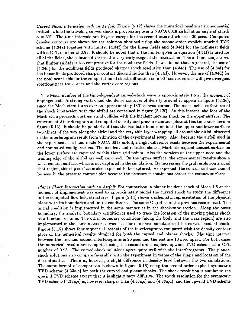
Curved Shock Interaction with an Airfoil: Figure (5.12) shows the numerical results at six sequential
instants while the traveling curved shock is progressing over a NACA 0018 airfoil at an angle of attack
= 30 °. The time intervals are 10/zsec except for the second interval which is 20/_sec. Computed
density contours are shown for the solution obtained using the second-order explicit upwind TVD
scheme (4.34a) together with limiter (4.34f) for the linear fields and (4.34d) for the nonlinear fields
with a CFL number of 0.98. It should be noted that if the limiter given in equation (4.34f) is used for
all of the fields, the solution diverges at a very early stage of the interaction. The authors conjectured
that limiter (4.34f) is too compressive for the nonlinear fields. It was found that in general, the use of
(4.34d) for the nonlinear fields produced sharper shock resolution than (4.34c). The use of (4.340 for
the linear fields produced sharper contact discontiniuties than (4.34d). However, the use of (4.34d) for
the nonlinear fields for the computation of shock diffraction on a 90 ° convex corner will give divergent
solutions near the corner and the vortex core regions.
The Mach number of the time-dependent curved-shock wave is approximately 1.5 at the moment of
impingement. A strong vortex and the dense contours of density around it appear in figure (5.12e),
since the Mach stem turns over an approximately 180 ° convex corner. The most inclusive features of
the shock interaction with the airfoil are contained in figure (5.12f). At this instant, the foot of the
Mach stem proceeds upstream and collides with the incident moving shock on the upper surface. The
experimental interferogram and computed density and pressure contour plots at this time are shown in
figure (5.13). It should be pointed out that the two little bumps on both the upper and lower surfacestwo thirds of the way along the airfoil and the very thin layer wrapping all around the airfoil observed
in the interferogram result from vibration of the experimental setup. Also, because the airfoil used in
the experiment is a hand-made NACA 0018 airfoil, a slight difference exists between the experimental
and computed configurations. The incident and reflected shocks, Mach stems, and contact surface on
the lower surface are captured within three grid points. Also the vortices at the upper nose and the
trailing edge of the airfoil are well captured. On the upper surface, the experimental results show a
weak contact surface, which is not captured in the simulation. By increasing the grid resolution around
that region, this slip surface is also expected to be captured. As expected, the contact surfaces cannotbe seen in the pressure contour plot because the pressure is continuous across the contact surfaces.
Planar Shock Interaction with an Airfoil: For comparison, a planar incident shock of Mach 1.5 at the
moment of impingement was used to approximately model the curved shock to study the difference
in the computed flow field structures. Figure (5.14) shows a schematic representation of the physical
plane with its boundaries and initial conditions. The same C-grid as in the previous case is used. The
initial condition is implemented in the same manner as in the shock-tube section. Along the outer
boundary, the analytic boundary condition is used to trace the location of the moving planar shock
as a function of time. The other boundary conditions (along the body and the wake region) are also
implemented in the same manner as was used for numerical simulation of the curved incident shock.
Figure (5.15) shows four sequential instants of the interferograms compared with the density contourplots of the numerical results obtained for both the curved and planar shocks. The time interval
between the first and second interferograms is 20/zsec and the rest are 10/zsec apart. For both cases
the numerical results are computed using the second-order explicit upwind TVD scheme at a CFL
number of 0.98. The curved-shock solutions agree quite well with the interferograms. The planar-
shock solutions also compare favorably with the experiment in terms of the shape and location of the
discontinuities. There is, however, a slight difference in density level between the two simulations.
The same format of comparison is shown in figure (5.16) using the second-order explicit symmetric
TVD scheme (4.33a,e) for both the curved and planar shocks. The shock resolution is similar to the
upwind TVD scheme except that it is slightly more diffusive. The shock resolution for the symmetric
TVD scheme (4.33a,e) is, however, sharper than (4.33a,c) and (4.33a,d), and the upwind TVD scheme
54
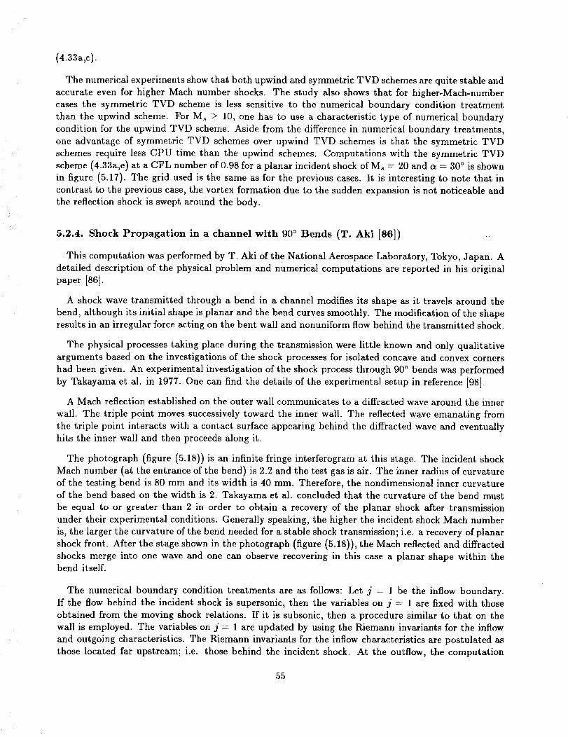
(4.33a,c).
The numerical experiments show that both upwind and symmetric TVD schemes are quite stable and
accurate even for higher Mach number shocks. The study also shows that for higher-Mach-number
cases the symmetric TVD scheme is less sensitive to the numerical boundary condition treatment
than the upwind scheme. For Ms _> 10, one has to use a characteristic type of numerical boundary
condition for the upwind TVD scheme. Aside from the difference in numerical boundary treatments,one advantage of symmetric TVD schemes over upwind TVD schemes is that the symmetric TVD
schemes require less CPU time than the upwind schemes. Computations with the symmetric TVD
scheme (4.33a,e) at a CFL number of 0.98 for a planar incident shock of Ms -- 20 and c_ -- 30 ° is shown
in figure (5.17). The grid used is the same as for the previous cases. It is interesting to note that in
contrast to the previous case, the vortex formation due to the sudden expansion is not noticeable and
the reflection shock is swept around the body.
5.2.4. Shock Propagation in a channel with 90 ° Bends (T. Aki [86])
This computation was performed by T. Aki of the National Aerospace Laboratory, Tokyo, Japan. A
detailed description of the physical problem and numerical computations are reported in his original
paper [86].
A shock wave transmitted through a bend in a channel modifies its shape as it travels around the
bend, although its initial shape is planar and the bend curves smoothly. The modification of the shaperesults in an irregular force acting on the bent wall and nonuniform flow behind the transmitted shock.
The physical processes taking place during the transmission were little known and only qualitative
arguments based on the investigations of the shock processes for isolated concave and convex corners
had been given. An experimental investigation of the shock process through 90 ° bends was performed
by Takayama et al. in 1977. One can find the details of the experimental setup in reference [98].
A Mach reflection established on the outer wall communicates to a diffracted wave around the inner
wall. The triple point moves successively toward the inner wall. The reflected wave emanating from
the triple point interacts with a contact surface appearing behind the diffracted wave and eventually
hits the inner wall and then proceeds along it.
The photograph (figure (5.18)) is an infinite fringe interferogram at this stage. The incident shock
Mach number (at the entrance of the bend) is 2.2 and the test gas is air. The inner radius of curvature
of the testing bend is 80 mm and its width is 40 mm. Therefore, the nondimensional inner curvature
of the bend based on the width is 2. Takayama et al. concluded that the curvature of the bend must
be equal to or greater than 2 in order to obtain a recovery of the planar shock after transmission
under their experimental conditions. Generally speaking, the higher the incident shock Mach number
is, the larger the curvature of the bend needed for a stable shock transmission; i.e. a recovery of planar
shock front. After the stage shown in the photograph (figure (5.18)), the Mach reflected and diffracted
shocks merge into one wave and one can observe recovering in this case a planar shape within thebend itself.
The numerical boundary condition treatments are as follows: Let j = 1 be the inflow boundary.If the flow behind the incident shock is supersonic, then the variables on j -- 1 are fixed with those
obtained from the moving shock relations. If it is subsonic, then a procedure similar to that on the
wall is employed. The variables on j -- 1 are updated by using the Riemann invariants for the inflow
and outgoing characteristics. The Riemann invariants for the inflow characteristics are postulated as
those located far upstream; i.e. those behind the incident shock. At the outflow, the computation
55
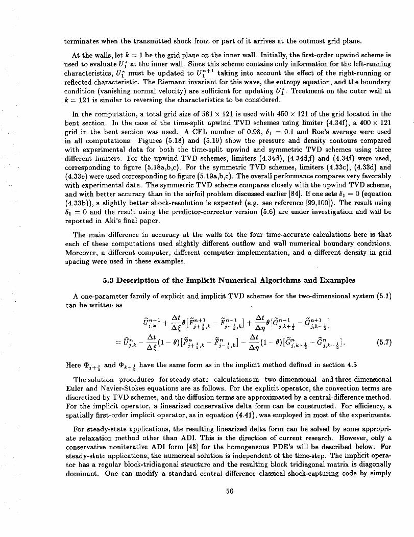
terminateswhenthetransmittedshockfront or part of it arrivesat the outmost grid plane.
At the walls, let k = 1 be the grid plane on the inner wall. Initially, the first-order upwind scheme is
used to evaluate U_ at the inner wall. Since this scheme contains only information for the left-running
characteristics, U_ must be updated to U_ +1 taking into account the effect of the right-running orreflected characteristic. The Riemann invariant for this wave, the entropy equation, and the boundary
condition (vanishing normal velocity) are sufficient for updating Ui_. Treatment on the outer wall at
k = 121 is similar to reversing the characteristics to be considered.
In the computation, a total grid size of 581 × 121 is used with 450 × 121 of the grid located in the
bent section. In the case of the time-split upwind TVD schemes using limiter (4.34f), a 400 × 121
grid in the bent section was used. A CFL number of 0.98, 51 -- 0.1 and Roe's average were used
in all computations. Figures (5.18) and (5.19) show the pressure and density contours compared
with experimental data for both the time-split upwind and symmetric TVD schemes using three
different limiters. For the upwind TVD schemes, limiters (4.34d), (4.34d,f) and (4.34f) were used,
corresponding to figure (5.18a,b,c). For the symmetric TVD schemes, limiters (4.33c), (4.33d) and
(4.33e) were used corresponding to figure (5.19a,b,c). The overall performance compares very favorablywith experimental data. The symmetric TVD scheme compares closely with the upwind TVD scheme,
and with better accuracy than in the airfoil problem discussed earlier [84]. If one sets 51 = 0 (equation
(4.33b)), a slightly better shock-resolution is expected (e.g. see reference [99,100]). The result using
51 = 0 and the result using the predictor-corrector version (5.6) are under investigation and will be
reported in Aki's final paper.
The main difference in accuracy at the walls for the four time-accurate calculations here is that
each of these computations used slightly different outflow and wall numerical boundary conditions.
Moreover, a different computer, different computer implementation, and a different density in grid
spacing were used in these examples.
5.3 Description of the Implicit Numerical Algorithms and Examples
A one-parameter family of explicit and implicit TVD schemes for the two-dimensional system (5.1)can be written as
",k A_ [" J'+l'k -- _3"--l'kJ + A_ 7 L--'7"'k+l --''i,k-½J
F_- _,k] - _) [G_,k+½ _.]- (5.7)= - - [ _+½,k _--_ (1 j,k-o) --" - -
Here Cj+½ and Ck+½ have the same form as in the implicit method defined in section 4.5
The solution procedures for steady-state calculations in two-dimensional and three-dimensionalEuler and Navier-Stokes equations are as follows. For the explicit operator, the convection terms are
discretized by TVD schemes, and the diffusion terms are approximated by a central-difference method.
For the implicit operator, a linearized conservative delta form can be constructed. For efficiency, a
spatially first-order implicit operator, as in equation (4.41), was employed in most of the experiments.
For steady-state applications, the resulting linearized delta form can be solved by some appropri-ate relaxation method other than ADI. This is the direction of current research. However, only a
conservative noniterative ADI form [43] for the homogeneous PDE's will be described below. For
steady-state applications, the numerical solution is independent of the time-step. The implicit opera-
tor has a regular block-tridiagonal structure and the resulting block tridiagonal matrix is diagonally
dominant. One can modify a standard central difference classical shock-capturing code by simply
56
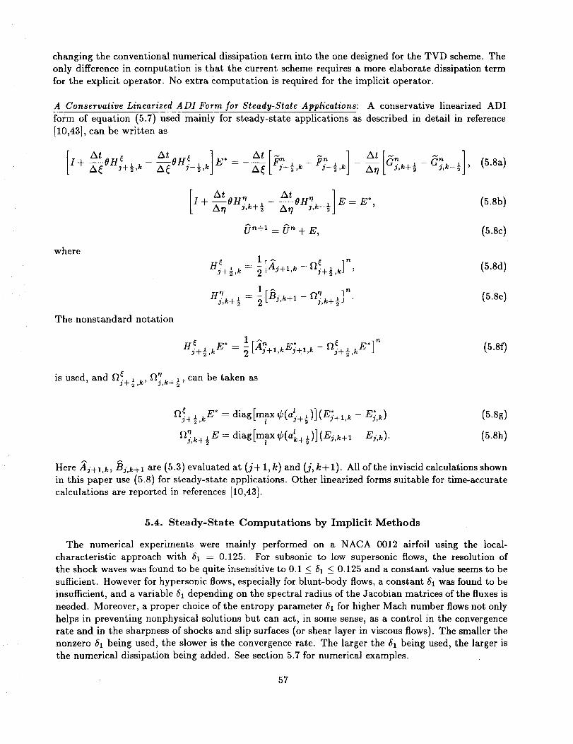
changingthe conventionalnumericaldissipationterm into the onedesignedfor the TVD scheme.Theonly differencein computationis that the current schemerequiresa moreelaboratedissipationtermfor the explicit operator.Noextracomputationis requiredfor the implicit operator.
A Conservative Linearized ADI Form for Steady-State Applications: A conservative linearized ADI
form of equation (5.7) used mainly for steady-state applications as described in detail in reference
[10,43], can be written as
- _ _ _ N° (5.8a)I+ A_ _+_,_ /_ FJ+_,k 3-_,k S_ j,k+_ ,
where
The nonstandard notation
At _ At OH _ ] E*I + --_OH/,k+ ½ Arl j,k-½ E = ,
,k 2 3"+1,k -- ½,k '
Ha?,k+½ 1 [_a. k+, '1 n= _ - n_+_]
(5.8b)
(5.8c)
(5.8d)
(5.8e)
E, 1 A}% *
H_+½,k = 2 [Aj+I,kEj+I, k - f_3"+½,_ "E*]nJ (5.8f)
is used, and _f2j+½,k' f_j,k+½' can be taken as
f23.+½,kE_• __ diag [max ¢(a_+½)] (E_+I, k - E_.,k)*
f2'_j,k+_ E= diag [max¢(a_ +½ )] (Ej, k+l- Ej,k).
(5.8g)
(5.8h)
Here/_j+l,k, Bj,k+l are (5.3) evaluated at (j+l, k) and (j, k+ 1). All of the inviscid calculations shown
in this paper use (5.8) for steady-state applications. Other linearized forms suitable for time-accurate
calculations are reported in references [10,43].
5.4. Steady-State Computations by Implicit Methods
The numerical experiments were mainly performed on a NACA 0012 airfoil using the local-
characteristic approach with 81 = 0.125. For subsonic to low supersonic flows, the resolution of
the shock waves was found to be quite insensitive to 0.1 _< 81 _< 0.125 and a constant value seems to be
sufficient. However for hypersonic flows, especially for blunt-body flows, a constant 81 was found to be
insufficient, and a variable 81 depending on the spectral radius of the Jacobian matrices of the fluxes is
needed. Moreover, a proper choice of the entropy parameter 51 for higher Mach number flows not only
helps in preventing nonphysical solutions but can act, in some sense, as a control in the convergence
rate and in the sharpness of shocks and slip surfaces (or shear layer in viscous flows). The smaller thenonzero 81 being used, the slower is the convergence rate. The larger the 81 being used, the larger is
the numerical dissipation being added. See section 5.7 for numerical examples.
57
Generally, for inviscid time-accurate calculations, upwind TVD schemes produce sharper shocks
than symmetric TVD schemes [8]. For the current implicit symmetric TVD scheme with limiter
(4.33c) or (4.33d), this seems to be not the case. The symmetric method appeared to produce almost
identical results as those from an upwind TVD scheme (4.34a)-(4.34c).
Numerical studies also show that there is no difference in resolution in using limiter (4.33c) or
(4.33d) for the symmetric TVD scheme. Limiter (4.33e) produces slightly sharper shocks than (4.33c)
and (4.33d). This conclusion was based on a numerical study for flow-field conditions ranging fromsubcritical to transonic and supersonic for the NACA 0012 airfoil. Also, since these test cases consist
of shock waves only, the same limiter was used for all characteristic fields. Figures (5.20) and (5.21)
show a comparison of the current method using limiter (4.33c) with the upwind scheme (5.1) for
two inviscid steady-state airfoil calculations. The two solutions are almost indistinquishable. For thecurrent calculations, the upwind TVD scheme requires approximately 35% more CPU time than the
symmetric TVD scheme on the CrayX-MP computer.
Figures (5.22) and (5.23) show an inviscid comparison of the symmetric TVD scheme with the widely
distributed computer code ARC2D, version 150 [101]. The free stream Mach numbers are M_ = 1.2
and 1.8, and the angle of attack is _ = 7 °. The pressure coefficient distributions (not shown) are
identical between the two methods and yet the flow field appears very different. The symmetric TVD
scheme gives a very well-ordered flow structure and can still capture the shocks with a coarse grid,
especially near the trailing edge of the airfoil. On the other hand, the ARC2D code did rather poorly.
The ARC2D, version 150 computer code is based on the Beam and Warming ADI algorithm [17], but
uses a mixture of second and fourth-order numerical dissipation terms. These numerical dissipation
terms contain adjustable parameters. The values of the parameters on figures (5.22) and (5.23) are
the same value as suggested in reference [101]. Other values of the parameters besides the one used in
reference [101] were also studied. What is shown here is representative of the performance of ARC2D
for this range of Mach numbers and angles of attack. For subsonic and transonic flow regimes the main
advantage of TVD schemes over ARC2D for steady-state calculations is that one can capture the shock
in one to two grid points as oppose to three to four. The flow away from the shock looks very much
like that calculated by ARC2D. Note that in general, for two-dimensional blast wave calculations, the
symmetric schemes usually can capture the shock in two to three grid points, but the slip surfaces are
slightly more diffusive than the upwind TVD schemes as discussed in section 5.1.
The same problem was studied for the upwind TVD scheme, and the results and convergence rates
were found to be almost identical to those for the symmetric TVD scheme. For figures (5.22) and(5.23), a residual of 10 -12 can be reached at about 400-600 steps. ARC2D, however, required only
200-300 steps to converge to the same residual.
Steady-state computations for higher Mach number flows in the hypersonic regime are currently
under investigation. Preliminary study shows that the ADI form of the implicit scheme is very sen-
sitive to initial conditions and numerical boundary condition treatments for blunt-body flows. The
convergence rate is lower than subsonic and supersonic flows.
5.5. A Thin-Layer Navier-Stokes Calculation
For steady-state application, a simple algorithm utilizing the TVD scheme for the Navier-Stokes
equations is to difference the hyperbolic terms the same way as before, and then central difference
the viscous terms. The final algorithm is the same as equation (5.8) except that the spatial central
differencing of the viscous term is added to the right-hand side of equation (5.8). The numerical
solution shown below illustrates that this algorithm produces a fairly good solution for the case of an
RAE 2822 airfoil calculation. Figure (5.24) is an example of the viscous case for the RAE 2822 airfoil
58

usingthe implicit upwindTVD schemeusinglimiter (4.34c).Thethin-layerNavier-Stokesequationswith the algebraicturbulencemodelof BaldwinandLomax[102]areused,andthetransition is fixedat 3%of chord.Theoverallagreementwith experimentsisquite good.TheL2-norm residual of 10-7can be reached in about 900 steps.
5.6. A 3-D Steady-State Computations by a Point-Relaxation Implicit Method [103]
Figure (5.25) shows pressure contours and energy contours in the plane of symmetry of the Aeroassist
Flight Experiment (AFE) configuration at V_ = 1429 m/s, p_ = 60.136 N/m 2, Too = 52.22°K,
T_o = 300°K, and Moo = 9.86. The configuration is a raked, elliptic cone with a circular shoulder.
The body has a circular cross section when viewed perpendicular to the raked plane. The vehicle
is designed as a test platform for a comprehensive series of experiments to define the flow field of
an Aeroassisted Orbital Transfer Vehicle (AOTV) at high altitudes (above 75 km) returning from aGeosynchronous Earth Orbit (GEO).
The numerical method employs a finite-volume, point-relaxation implicit procedure of the symmetric
TVD formulation (limiter (4.33d)) of the governing Navier-Stokes equations. Gauss-Seidel iteration
is employed across data planes in the sweep direction (from the body, accross the captured shock tothe inflow boundary and back). Jacobi relaxation is used with respect to discretization within a single
data plane. At each cell interface, Roe's averaging is used to define eigenvectors and eigenvalues, and
81 is set to a constant value of 0.2. Courant numbers up to 40 can be used to accelerate convergence.
But Courant numbers of 1 to 2 must finally be used to damp high-frequency errors. The grid size
(at close to the converged solution) was 64 cells between the body and the inflow boundary, 39 cellsfrom the nose to shoulder, and 19 cells around the axis from 0 ° to 180 °. The bow shock in this case
is almost completely captured in two cells.
5.7. The Entropy Condition and Blunt-Body Hypersonic Flows
For Mach number ranges from 1.2 to 15, numerical experiments for one- and higher-dimensional
unsteady flows containing unsteady shocks show that the second-order explicit TVD schemes via the
local-characteristic approach are insensitive to the entropy correction for 0 _< _i1 < 0.1 in equation
(3.18). In most cases _il -- 0 was used. For 0.1 _< _1 _< 0.25, it has the effect of smearing the
discontinuities slightly and sometimes has the advantage of improving stability in the sense of allowinga higher CFL number.
For steady-state computations, 0.01 _<(_1 _( 0.125 is a commonly used range for 0.6 < M < 4. The
more complex formula suggested in reference [32] was also employed but shows no visible difference
in shock resolutions or improvement in convergence rate when compared with the constant _1.
For blunt-body steady-state flows with M > 4, the initial flow conditions at the wall are obtained
using the known wall temperature in conjunction with pressures computed from a modified Newtonian
expression. Also, for implicit methods, a slow startup procedure from free stream boundary conditions
is necessary. Most importantly, it is advisable to use _1 as a function of the velocity and sound speed.
In particular
(5.9a)
(_l)k-t-½ = I+ Irk+½1+ (5.9b)
with 0.05 _< _ _< 0.25 appears to be sufficient for the blunt-body flows for 4 _< M <_ 25. Equation
59
(5.9) is written in Cartesian coordinates. In the case of generalized coordinates, the u and v should be
replaced by the contravariant velocities, and one half of the sound speed would be from the _-direction
and the other half would be from the r/-direction. For implicit methods, it is very important to use
(5.9) in ¢(z) on both the implicit and explicit operators. For the implicit operator, instead of usingl
(5.9) for ¢(z), numerical experiments showed that replacing the maxl ¢(aj+½) and maxl ¢(a_+½)
in equations (5.8g) and (5.8h) by
luj+ I+ Lvj+ l + c +½ (5.10a)
luk+ L + Ivk+ I+ ck+ (5.10b)
performed well for high Mach number blunt-body flows. Again, in the case of generalized coordinates,
the u, v and c in (5.10) should be the corresponding transformed coordinate variables.
Numerical experiments (perfect and equilibrium real gases) [104,105] for either explicit or implicit
methods showed that increasing the coefficient _ has the effect of speeding up the convergence rate
but smears the discontinuities slightly, since the bigger the _, the larger the numerical dissipations
being added. One way of improving the convergence rate (without employing additional relaxation
methods or multigrid procedures but retaining sharpness of the discontinuities) is to first use a larger
in the range of 0.15 __ _ < 0.4 to obtain a converged solution and then use 0.01 < _ < 0.15 as a
postprocessor to obtain better resolution at discontinuities. Figures (5.26) and (5.27) show examples
of two-dimensional steady-state blunt-body results. Figure (5.26) is a viscous computation and figure
(5.27) is an inviscid, equilibrium, real-gas computation using (5.9). Details of the computations and
related numerical examples can be found in references [104,105]. The following are short descriptions
of the numerical results for figures (5.26) and (5.27).
Figure (5.26) shows the Mach contours computed by the explicit MacCormack method and the
implicit symmetric TVD scheme (5.8) using limiter (4.33c) of a viscous shock on shock interaction
on a blunt cowl lip in the low hypersonic range. Extensive study on flow fields of this type were
reported in references [106-108]. The computed result by shock-fitting for the outer bow shock and
MacCormack methods for the interior of reference [107] is illustrated here for comparison. This flow
field is typical of what will be experienced by the inlet cowl of the National Aerospace Plane (NASP).
The free stream conditions for this flow field are Moo = 4.6, Reno_ = 10,000, Pr _ 0.72, poo = 14.93
N/m, Too = 167°K, T_ = 556°K, and _/ -- 1.4 for a perfect gas. An oblique shock with an angle
of 20.9 ° relative to the free stream impinges on the bow shock. Various types of interactions occur
depending on where the impingment point is located on the bow shock. As shown by the Mach
contours, the impinging shock has caused the stagnation point to be moved away from its undisturbed
location at the symmetry line. The surface pressures and heat transfer rates at the new stagnation
point can be several times larger than those at the undisturbed location of the stagnation point. In
addition, a shear layer emanates from the bow shock and impinging shock intersection point and is
intercepted by a shock wave which starts at the upper kink of the bow shock. The interacting shock
waves and shear layers are confined to a very small region and must he captured accurately by the
numerical scheme if the proper surface pressures and heat transfer rates are to be predicted correctly.
The convergence rate using scheme (5.8) in this case is many times slower than the airfoil calculations
discussed in section 5.4. The grid size for the MacCormack method is 51 × 31 and for the symmetric
TVD is 151 × 71. The computational domain and number of grid points are larger for the symmetric
TVD method than those for the MacCormack method, since the bow shock is also captured by the
scheme.
6O
Figure (5.27) shows the density contours computed by a second-order, non-MUSCL, upwind TVD
scheme (4.40) using limiter (4.34c) of an inviscid blunt-body flow in the hypersonic equilibrium real
gas range. The free stream conditions for this flow field are Moo -- 25, poo = 1.22 x 10³ N/m 2,
poo -- 1.88 -2 kg/rn s, and Too = 226°K. The grid size is 61 × 33 for the full (half) cylinder. The shock
is at approximately fourteen points from the wall on the symmetry axis. The relaxation procedure
employs a second-order Runge-Kutta method with a CFL of 0.5. The generalized Roe's average [57] is
used to define eigenvectors and eigenvalues, and _ is set to a constant value of 0.15. Figure (5.27) shows
the solution at 5000 steps with a four order of magnitude drop in the L2-norm residual. Pressure and
Mach number contours converge and stabilize after 3000-4000 steps but the convergence rate is much
slower for the density. The bow shock is captured in two to three grid points. Since the temperature
of this problem can go up to 8100°K and the curve fits of Srinivasan et al. [89] used are accurate only
for temperatures up to 6000°K, there is an uncertainty in the accuracy of the computed result andfurther investigation is needed.
In summary, steady-state computations for higher Mach number, blunt-body flows in the hypersonic
regime are very sensitive to initial conditions and numerical boundary treatments. A proper choice
of the entropy parameter _1 for higher Mach number flows not only helps in preventing ,nonphysicalsolutions but can act as a control of the convergence rate and helps in the resolution of discontinuities.
61

VI. Efficient Solution Procedures for Large Systems with Stiff Source Terms [99]
In the application of modern shock-capturing methods like the TVD type of schemes to the chemi-
cally reacting flows, Carofano [81] was the first to introduce the formalism that enabled full coupling
in Harten's explicit TVD scheme for a two-species, two-dimensional unsteady flow in Cartesian co-ordinates. However, due to the system size and the varying time-scale nature of the problem, the
operations count increases nonlinearly as the number of species increases. To avoid solving a large
system, Gnoffo and McCandless [109] and Gnoffo et al. [103] uncoupled the species equations from
the fluid dynamics equations and solved these two sets of systems of nonlinear partial differential
equations in a time-lag fashion (loosely coupled method) by using a point-relaxation technique with
a second-order symmetric TVD scheme of Yee [10,87] and an upwind TVD scheme of Osher and
Chakravarthy Ill]. Eberhardt and Brown [110] attempted to use the eigenvalues and eigenvectors of
the fluid dynamics equations alone to obtain a "fully coupled" first-order explicit TVD scheme for aone-dimensional flow. The results of Eberhardt and Brown showed excessive smearing at the shock
when compared with the true, fully coupled explict TVD result. Their motivation for designing such a
coupling procedure was to optimize the operations count by avoiding multiplication of large matrices.
However, as will be demonstrated below, if one makes use of the unique structure of eigenvectors and
eigenvalues for fluid flow of this type, the fully coupled formulation can be simplified even for a large
number of species, thus providing a more efficient solution procedure than one might have anticipated.
Moreover, using the eigenvalues and eigenvectors for the fully coupled equation set allows one to have
the freedom of controlling the proper amount of numerical dissipation for the individual waves [10].
In particular, for the two-dimensional chemically reacting flows, the number of linear waves is ns + 1
in each spatial direction where ns is the number of linearly independent species. Note that in or-
der to capture contact discontinuities accurately, it is very important to apply the proper amount of
numerical dissipation to the linear waves.
Two types of schemes are proposed. If the stiffness is entirely dominated by the source term, a semi-
implicit TVD type of shock-capturing method is proposed for steady-state calculations provided that
the Jacobian of the source terms possesses certain properties. The proposed semi-implicit scheme can
be viewed as a variant of the Bussing and Murman point-implicit predictor-corrector scheme [50] with
a more appropriate numerical dissipation for the computation of strong shock waves in the hypersonic
regime and a speed up in the convergence rate for steady-state applications. The predictor-correctorscheme of Bussing and Murman in turn is the explict MacCormack scheme with the source term
treated implicitly.
However, if the stiffness is not solely dominated by the source terms (e.g., stiffness due to highly
irregular grid and/or viscous flows), a fully implicit method would be a more efficient procedure. Thesituation is complicated by problems in more than one space dimension, and the presence of stiff source
terms further complicates the solution procedures for alternating direction implicit (ADI) methods. In
fact, there seems to be no straightforward way of efficiently treating general stiff source terms implicitlywith ADI procedures. Several alternatives will be discussed. The proposed fully implicit relaxation
algorithm can be viewed as a variant of a fully coupled form of the algorithm proposed by Gnoffo and
McCandless [109]. An implicit algorithm with explicit coupling between fluid and species equations
proposed by the author will also be stressed here. Many existing perfect-gas or equilibrium real-gas
computer codes can easily be modified to include this algorithm, which is a compromise between the
loosely coupled implicit method of [109] and the fully coupled, fully implicit TVD method proposed
here. To make this section more self-contained, some of the variables that were defined earlier will be
repeated.
62
6.1. An Explicit Predictor-Corrector Algorithm for Systems with Source Terms
In this section, all the necessary terms that are required for the basic TVD scheme for the com-
pressible inviscid chemically reacting flow equations are derived.
The Governing Equations: Consider a two-dimensional system of nonhomogeneous hyperbolic conser-vation laws,
OU OF(U) OG(U) _ S(U). (6.1)o-T+ o---_+ o_
Here U, F(U), G(U), and S(U) are column vectors of k components. Let A : OF/OU and B :
2 k 2 ...,a_) being the eigenvalues of A and B. Denote R_ and R_OG/OU, with (a_,a::,...,a_) and (al,ay,
as the matrices whose columns are eigenvectors of A and B, and denote R_ 1 and R_ -x as the inversesof R_ and Ru. In the case of the compressible inviscid flow equations with chemical reactions, the
global continuity equation is replaced by the individual species continuity equations,
"pl -
p2
U : . ; F(U)=
pnS
m
n
clrn cln .81 '
c2m c2n 82
; C(V)= ; s(v)=enSm enS n 8ns
7 +P -V o71_ n n 2
_-+p 0
(6.2)
p
e (e+p)_ (e+p)_ 0
Here rn = pu, n = pv, and s_ represents the production of species from chemical reactions• The
variables are the velocity components u and v, the pressure p, the total energy per unit volume e, and_'_ns pi " "the density of the ith species p'. Also, p = z-_i=l and c*p = f, where ns is the number of species in
the model and ci is the species mass fraction. Equation (6•2) assumes the pi are linearly independent.
The eigenvalues of A and B are
a 1 a_ s+s)( _,..., :(u,...,u,u+a,u,u-a), (6.3a)
(al_, a '_s+3) = (v, ..., v, v + a, v, v - a)."", y
Here the so called "frozen sound speed" a is
(6.3b)
a 2 = pp +pe(H- u 2 - v2), (6.4)
with
ns i (6.5)p_: 2_.,,:cp_,,c'= 1, (6.6)
i=l
0p m,.,_.... (6.7)pp_ = Op i
pe= _ , (6.8)OelmWt,pl,.. *
63
S - e+ p (6.9)
The frozen sound speed a defined in (6.4) has no physical meaning. It is defined here for the convenience
of notation for the basic scheme.
The superscript n is used for the time-index and should not be confused with the n = pu in equation
(6.2). Let al+3 _ ' Rj+ ½, Rj+½-1 denote the quantities a_,Z R,:, R_ 1 evaluated at some symmetric average
L Ru, evaluated at-1 denote the quantities ay, R_-Iof Ui, k and Uj+l,k. Similarly, let a_+½, Rk+½, Rk+ ½
some symmetric average of U3,k and Uj, k+l. In the case of chemically reacting flows, aj+½, Rj+½,
-1 elk+½, and -1R ._,, Rk+ ½, Rk+ ½ are defined in ways similar to the ones used by Huang [30] and Carofano
[81]. Also, although the commonly used Roe's average is no longer valid for a nonperfect gas, a close
approximation based on a generalized Roe's average for equilibrium flows as discussed in section 4.3
and reference [57] can also be used.
For thermally and chemically nonequilibrium flows, the eigenvalues and eigenvectors have a similar
structure. For the two-dimensional system (6.1), if nt is the number of thermal energy variables, then
the eigenvalues in the x-direction will have (ns + nt + 1) "u" characteristics plus u + a and u - a
characteristics. Here the values "a" will reflect the added thermal energy variables
As discussed in sections 3.3, 3.6, and 3.7, the TVD property is only valid for homogeneous scalar
hyperbolic conservation laws. Certain types of source terms might preserve the original TVD property
of the homogeneous PDE, and others might not. However, disregarding the type of bounded source
terms, one is not precluded from the application of TVD schemes when source terms are present.
But, extreme precaution has to be taken (especially for explicit TVD schemes) in the procedure of
including the source terms. This applies particularly to stiff source terms of the types in thermally
and chemically nonequilibrium flows. Procedures for time-accurate computations for problems with
stiff source terms are currently under investigation. However, in the use of time-accurate methods as
relaxation procedures for steady-state computations, the semi-implicit algorithm discussed in section
3.7 appears to work quite well.
Explicit Preditor-Corrector TVD Scheme: With the above notation, a formal extension of the scalar
explicit second-order TVD method (section 3.6) in predictor-corrector form via the local-characteristic
approach for the nonlinear hyperbolic system (6.1) with nonzero source terms can be written as
AU_"k -- _-x 3,k- F;-1,k - _y Gj,k+ 1 -GJ, k -_- AtS_, k' (6.10a)
1 { (1) At
g(1)= Au}lk ) + U n (6.lOb)./,k , a,k,
_. [F_+)l,k- Fa,,1,] - At (1)}, (6.10c)
U(2) (2) U(1) (6.10d)j,k = AU_,k + j,k,
"" '=' ' 3-2 3-_j _ k-_ k-_]"
The elements of the vector (I)j.+½ are the same as equations (3.59d) and (3.59e) with %.+½ replacedl ^ ^l
by a t A+½ replaced by aj+½ and Q_.+½ replaced by Qj+½. Here Ay is the grid spacing such3"+½'
64

that Yk : kAy. Research is underway to study the influence of the stiff source terms on the TVD
correction step for the second and third terms of (6.10e) to be evaluated at u n compared with (6.10e).
For steady-state calculations and for a contractive type of source term S(U), it appears that (6.10e)
might helped improve the convergence rate by using the most updated information in the relaxation
procedure. Other procedures are currently under investigation.
6.2. More Efficient Solution Procedures for Large Systems
The extra computation in (6.10) compared with a classical central-difference shock-capturing scheme
such as the Lax-Wendroff method is due to the vectors (R(I))j±½. At first glance, the vectors aj+½
and (R(I))j+ ½ involve matrix and vector multiplication of dimension ns + 3 for every grid point, and
thus tend to discourage their adoption in problems other than ideal gas flows. Researchers such as
Gnoffo and McCandless [109], and Eberhardt and Brown [110] were motivated to pursue other avenues
to solve the complicated chemically reacting flow problems. However, as will be demonstrated in this
subsection, if one makes use of the unique structure of the eigenvectors and eigenvalues for fluid flow
of this type, the fully coupled formulation can be simplified even for a large number of species, and
thus becomes a viable approach.
With straightforward manipulations, the computation for scheme (6.10) can be simplified tremen-
dously. The corresponding vector a in equation (4.12c) for system (6.1)-(6.2), for example, can be
expressed as
OL ----
Ap 1 - claa
Ap 2 -- c2aa
Ap ns _ cnSaa
l(aa :bb+ A_)-
!(_vbb + An)a
l(aa+ :bb A_)-_
(6.11)
with
aa = _ff i=lpp_ Ap_ - p_(uArn ÷ vAn - Ae , (6.12)
_-_n:l AP "- ( )bb -- ' 6.13
p_Here, for example, (Ap)j+½,k = j+l,k - Pj,k, and it is understood that the spatial indices in (6.11)-lk(6.13) are at (j ÷ _, ). Similarily, R¢ also has a very simple form. For instance, the R(I) associated .
with the x-direction flux can be expressed as
65

with
RO=
Cns __ cnSkl
uk2 + ks
vk2 + a¢ "_+2
1N-'ns (ai)20 i +av¢ ns+2 _-uk3Hk2 - p,,z..,i=l
kl = ¢.8+1 + ¢._+_,
_--...,ns+3 i
k2 = ___i=l,iCns÷2(_ ,
ks = a(¢ ns+l - Cns+3).
(6.14a)
(6.14b)
(6.14c)
(6.14d)
Here the spatial indices on (6.14) are at (j + 1 ]¢_, ). As one can see, the terms in equations (6.11) and
(6.14) due to the species equations are simple and do not require many operations. Therefore, theincrease in the number of species equations is not as CPU-intensive as one might have anticipated.
6.3. A Semi-implicit Predictor-Corrector TVD Algorithm and a 3-D Example
As mentioned in discussing the scalar schemes, the explicit TVD scheme (6.10) can be used for either
time-accurate or steady-state calculation. It is second-order accurate in time and space. However, if
the source term is stiff, the restriction in the time-step due to stability requirements is prohibitively
small and (6.10) is not practical, especially for steady-state applications where a large system such
as (6.2) is involved. In this section, a semi-implicit method is proposed. Another alternative is a
fully implicit method. The basic implicit scheme and the related difficulty in efficiently extending the
implicit method to two dimensions with stiff source terms will be discussed in the next section.
If one follows the idea of Bussing and Murman [50] in treating the source term implicitly, a semi-
implicit predictor-corrector TVD algorithm for steady-state computations can easily be obtained. It
can be written as a one-parameter family of time-differencing schemes for the source term; i.e., the
following formulation includes scheme (6.10). The proposed scheme for system (6.1) can be written as
j,k,_,v.k = -_x_F_,k- F_.n_l,k - -_y aj, k+ 1 --a3. k -_- ItS?k , (6.15a)
D= (I- AtOO_U), (6.15b)
D(1)AU(2 ) 1 f_AU!I) At [ ] i_ [G(1)e(.l) 1 Ats_lk )} (6.15c)= ,,k-ij ,, [ j,k
_j,krr_+l: U(2),,k+[ rR(2),+5' O(2',÷5' -R(2)"-½ O(2)]J-½+ [jR(2)_k+5 Ok+(2)5'- Ri2-) 10(2) £]5 k- . (6.15d)
Here, D is assumed to be invertible; i.e., only source terms with Jacobians such that D is invertible ateach grid point are permissible. Again, 0 has the same meaning as in the scalar case. For 0 # 0, the
66
sourcetermsaretreatedimplicitly. If 0 = 1, the time-differencing for the source term is first-order and
(6.15) is best suited for steady-state calculations. See sections 3.3, 3.6, 3.7 and 6.1 for the discussion
of equation (6.15d) and the usage of the scheme (6.15) in general.
One can simplify equation (6.15) by partitioning the vectors U, F, G, S, and D in equation (6.2) asfollows:
u 1
U ns
V II =
I Uns+ l
uns+ 2
uns_-3
(6.16a)
[F,] [oi]F= FII , G= GII , (6.16b)
I ] $IS= SH ; =
81
8 _8
SII (6.16c)
D n D 12 ]D= [O2 ` 022 • (6.16d)
Here D 21 is a null matrix and D 22 is an identity matrix. With the above definitions, the scheme can
be greatly simplified. The procedures are as follows: taking the predictor step, for example, one firstsolves for (AUII) (1) by
,F!, I ,, n ,,(/kU ),',k -- _ (F;llk) n -- ' ,'-l,k' -- _ (Gj,k+l) -- (Gj,k) , (6.17a)
then for (AUI) (1) by
Dll _nlAUl_(1) )I 12 - --lI'l(1)j,k! t Jj, k = (r.h-s - nj, k(Au )j,k, (6.17b)
where (r.h.s) I is the right:hand side of (6.17a) with all the indices "II" replaced by 'T', and with the
term At(SIk) n added. In other words, one only has to invert the 011 matrix of dimension (ns, ns)
instead of ins+ 3, ns + 3). Similarly, one can simplify the corrector step in the same way. The solution
obtained from the above procedure is used in (6.15d). Or, to explain it in another way, one solves thepredictor step of the fluid equations
OU H OFH(U) OGH(U)--+ + -0
at ax ay
explicitly, then uses the result to solve the predictor step of the species equations
oula----i-+ c_FI(U)o------_+ aGI(U)oy - sl (6.18b)
explicitly, with the exception that the chemical reaction terms are treated implicitly in (6.18b). Onethen repeats the same procedure for the first corrector step. The solution obtained from the first
(6.18a)
67

corrector step is then used to solve for c_ and Re in equations (6.11)-(6.14) for the complete system
(6.1) so that one can solve for the second corrector step. Here, the first corrector step means the step
to obtain U (2) from U (1), and the second corrector step means the step to obtain U n+l from U (2) in
(6.15). Note that the second corrector step is the important part of the algorithm that deviates from
the Bussing and Murman method. This step, which ensures that the method will have the TVD-type
properties, is designed to capture shock waves without the associated spurious oscillations.
In the case where S II is not a null vector and it is not stiff, equation (6.17) is still applicable, except
one has to add the term At(sjlI)" to the right,hand side of (6.17a). In steady-state calculations
where body-fitted coordinates are used, one can further speed up the convergence rate by using a local
time-stepping approach [18,101].
To verify the current approach and to make a fair comparison with a known method, the proposed
semi-implicit scheme was implemented into an existing three-dimensional code [111]. This existing full
Navier-Stokes code, originally developed by A. Kumar at NASA Langley Research Center, contains
the explicit MacCormack scheme with source terms treated implicitly. A detailed description of a
numerical experiment and the extension of (6.15)to three-dimensional, chemically reacting flows in
generalized coordinates is given in Shinn et al. [100]. Only partial results from reference [100] are
presented here to illustrate the performance of the proposed semi-implicit scheme. In reference [100],
three symmetric averages for the eigenvalues and eigenvectors were studied. Aside from a slight
difference in convergence history, no visible differences in resolution were observed among the different
averages. The computations shown employed _1 = 0.1 for the entropy correction function ¢(z) in
equation (3.18).
Figures (6.1)-(6.3) show a preliminary test result for a three-dimensional, five-species viscous re-
acting flow using the semi-implicit TVD scheme (6.15) together with (6.13f), as compared with an
existing classical shock-capturing method which supplies numerical dissipation linearly [111]. The
numerical result for the semi-implicit TVD method is shown to be oscillation-free around the shock,
while the time spent per iteration is approximately double when compared with the method used in
[111]. The configuration of the numerical experiment is shown in figure (6.1). Although this is a
two-dimensional flow, to check out the three-dimensional code it is computed as a three-dimensional
flow with the appropriate boundary conditions in the y-direction. A uniform grid consisting of 31
points in the x-direction, 6 points in the y-direction and a viscous grid consisting of 51 points in the
z-direction was used. The inflow conditions are the pressure p = 1 atm, the temperature T -- 1200 K,
and the Mach number M = 4 for a premixed air and hydrogen fuel. The species considered are H2,
02, OH, H20, and N_, with the two reactions (N2 being inert)
H_ ÷ 02 _- 20 H,
20H ÷ H2 _- 2H20.
The reaction rates for the above are given in reference [111].
6.4. A Fully Implicit TVD Method and a 3-D example
Another type of shock-capturing scheme that might be applicable to (6.1) is a one-parameter family
of explicit and implicit TVD-type of schemes (section 3). For the nonequilibrium equation (6.1), these
schemes can be written as
68
(6.19)
Here0 has the same meaning as before. The numerical fluxes Fj±½,k and Gj, k±½ have the same
meaning and form as the scheme for the homogeneous PDE's (5.1). Again, the MUSCL or non-
MUSCL approaches as discussed in section 4.5 for the implicit method are applicable here.
6.4.1 A Conservative Linearised Form For Steady-State Applications
To solve for U _+1 in (6.19), one normally needs to solve a set of nonlinear algebraic equations
iteratively. One way to avoid this is to linearize the implicit operator, and solve the linearized form
by other means. Following the same procedure as in section (3.8) and in Yet [10,43], a conservativelinearized form of (6.19) can be written as
(6.20a)
E -- U n+l - U", (6.20b)
where the H_+},k, _.H_.k+_' Fj+½,k and G_,k+½ have the same form as in equation (5.8) and section
(4.5) except all the vectors are in Cartesian coordinates.
6.4.2. Stiff Source Terms, ADI Approaches and Relaxation Methods
The stiff terms Dj_ on the implicit operator (6.20) complicate the solution procedures for the
commonly used ADI procedures. Normally, if Djn, k are not stiff, one can reformulate (6.20) by an ADI
procedure like the Beam and Warming [17] algorithm for an efficient solution process. Unfortunately,
the D_,k considered here is stiff; consequently the additional higher order terms due to the ADI
formulation can no longer be ignored. In a different context, Van Dalsem and Steger [112] suggested a
remedy if D_'_,k is a diagonal matrix with identical diagonal elements. However, for chemically reacting
flows, the matrix D3_k is full for the upper (ns, ns + 3) entities and no straightforward efficient way of
utilizing ADI approaches for nonlinear system cases with a general stiff source terms can be found.
The straightforward way of iteratively solving (6.19) as a set of nonlinear system of equations
iteratively, or solving the linearized form (6.20) or similar non-ADI forms, appears to be quite expensive
for large systems. Recently, Gnoffo et al. [103] successfully demonstrated the usefulness of a point-
relaxation method on the implicit symmetric TVD scheme similar to (6.20) for a loosely coupled
chemically nonequilibrium flow. Here a similar point-relaxation or line-relaxation method is proposed
for the fully coupled system (6.15). Despite the fact that a larger equation set is involved than in
[103], the extra operations are minimized by making use of the simplification procedure of section
6.2. For a point-relaxation method, the size of the matrix inversion for (6.20) is (ns + 3, ns + 3) as
opposed to the loosely coupled method of [103], where the size is (ns, us). The gain in the freedom
of controlling the appropriate amount of numerical dissipation for each individual wave more than
compensates for the extra expense. More importantly, solving the fully coupled system is believed to
have a better convergence rate than the loosely coupled approach. All of the necessary terms required
for the implicit_scheme (6.20) are derived in section II. The implicit operator of (6.20a) is diagonally
dominant for Dj,k = 0. Therefore, one has to make sure that the source term does not destroy
69

the diagonallydominantpropertywhich is requiredfor somerelaxationmethods. In the followingsubsection,anevensimplerform than (6.20)is proposed.
6.4.3. An Implicit Algorithm with Explicit Coupling between Fluid and Species Equa-
tions
To avoid the inversion of large matrices, one can further simplify (6.20) by requiring that the coupling
between the fluid and species equations be explicit. With this relaxed requirement, one effectively
solves the fluid and species equations separately. Unlike the loosely coupled method used in [103]
or the chemistry-split technique used in [113], the eigenvalues and eigenvectors of the fully-coupled
equations are coupled explicitly between the fluid and species equations. This can be accomplished by
partitioning U,F,G,S,-D in the same way as in (6.16) and partitioning the Jacobians A and B, and
the numerical fluxes Fj+½,k and Gj, ki½ similarly. For example, the Jacobian A and the numericalN
fluxes Fj+½, k can be partitioned as
A 1 A 12 ]A : [ A21 A22 , (6.21)
= NII •Fj ,k [
(6.22)
The dimensions of the subvectors and submatrices are the same as (6.16) if equation set (6.2) is chosen,
and the A n, A 12, A 21, and A 22 in this case are
A ll
tt(1 -- C 1)
-- uc 2
-- ¢tC ns
-- uC 1 -- Uc 1
u(1 - c 2) - _c 2
-- t_e ns u(1-c "8)
(6.23a)
A 12 =
C1 0 0
C2 0 0
C ns 0 0
(6.23b)
A 21 =
pp, - u 2
-- t_V
u(pp, - H)
pp2 -- u 2
-- try
u(pp2 - H)
A 22 =
2u -- upe
v
H - u2pe
-- vpe
u
-- uvpe
Similarly, Ej, k and 12_ can be partitioned as
P#"" -- U2 1
-- UV ]u(p,.. - H)
pe10
u(1 + pe)
(6.23c)
(623d)
7O
r_:--(re)"' (_:)":"
(6.24)
(6.25)
Recall that two choices of equation sets are available: namely, equation set (6.2), or the full fluid
equations (i.e., keeping the global continuity equation) plus the ns- 1 species equations. The procedure
suggested here is best suited for the latter equation set, since modification of many existing implicit
solver computer codes (perfect gases or equilibrium real gases) would be minimal. The dimensions of
subvectors and submatrices for the latter equation set would be slightly different. For example, the
dimensions for A 11, A 12, A 21, and A 2_ would be (ns - 1) × (ns - 1), (ns - 1) × 4, 4 × (ns - 1),and 4 × 4, respectively.
The procedures for either equation set are as follows. One solves the fluid equations (e.g., (6.18a))implicitly, and then uses the result (uH) n+l to solve the species equation (e.g., (6.18b)) implicitly. In
other words, one solves (UH) '_+1 from the following:
/ ["( " " ") "( " " .)")]}1 - (/-/_,k- E" (rhs) 1,, (6.26a)I+e _x (Hj+s,k) -(H_-½,k) +-_y (I-Pj,k+½) Y =
lI ~ IS] At [ _n II(rhs)SS - azAt (_+½,k) -(_-½,k) - _ [(G3.,k+½) _ (Gj,k__).~ szlj, (6.26b)
( _lX "_II 1 x 22 n:'j+½,k, = _[(Aj+l,k) 22 -(12j+½,k) ] (6.26c)
The explicit coupling between the fluid and species equations is imbedded in (6.26b). After obtaining
(U HV_+I from (6.26), the solution is used to solve the species equation as follows:].i,k
I+0
= (rhs)' - (Zhs)'_,
+ _-At .7.,k_½)s) At---" 1j.l
(6.27a)
with
= 2 Axx (AJ+a'k)t2 - (_"_J+½ ,k)i2 - (A3-l'k)12 -_ (_'_;-½, k)12
ri
12 y 12
At ((Bj, k-t-1) - (_*'_Yk_t 1)12 -- (B,,k-1)12 _- (__3. k_½) ) ] -- 0at(n_,#l:) 12) (6.27b)Esl
and
1 rt A _11 [_x _11] n (6.27c)(H]+_,k) s= _l_ _+l,kj -_ j+½,k, J •
The term (rhs) I is the right-hand side of (6.26b) with all the indices "II" replaced by 'T' and the source
term At(S_,k) I added. Here the quantities in equation (6.27) are evaluated with updated information
71
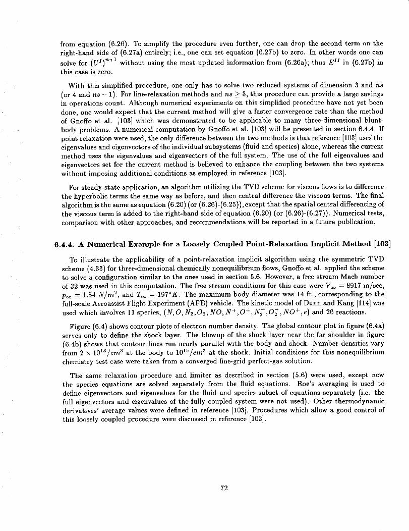
from equation (6.26). To simplify the procedure even further, one can drop the second term on the
right-hand side of (6.27a) entirely; i.e., one can set equation (6.27b) to zero. In other words one can
solve for (UI) "÷1 without using the most updated information from (6.26a); thus E xl in (6.27b) in
this case is zero.
With this simplified procedure, one only has to solve two reduced systems of dimension 3 and ns
(or 4 and ns - 1). For line-relaxation methods and ns > 3, this procedure can provide a large savings
in operations count. Although numerical experiments on this simplified procedure have not yet been
done, one would expect that the current method will give a faster convergence rate than the method
of Gnoffo et al. [103] which was demonstrated to be applicable to many three-dimensional blunt-
body problems. A numerical computation by Gnoffo et al. [103] will be presented in section 6.4.4. If
point relaxation were used, the only difference between the two methods is that reference [103] uses the
eigenvalues and eigenvectors of the individual subsystems (fluid and species) alone, whereas the current
method uses the eigenvalues and eigenvectors of the full system. The use of the full eigenvalues and
eigenvectors set for the current method is believed to enhance the coupling between the two systems
without imposing additional conditions as employed in reference [103].
For steady-state application, an algorithm utilizing the TVD scheme for viscous flows is to difference
the hyperbolic terms the same way as before, and then central difference the viscous terms. The final
algorithm is the same as equation (6.20) (or (6.26)-(6.25)), except that the spatial central differencing of
the viscous term is added to the right-hand side of equation (6.20) (or (6.26)-(6.27)). Numerical tests,
comparison with other approaches, and recommendations will be reported in a future publication.
6.4.4. A Numerical Example for a Loosely Coupled Point-Relaxation Implicit Method [103]
To illustrate the applicability of a point-relaxation implicit algorithm using the symmetric TVD
scheme (4.33) for three-dimensional chemically nonequilibrium flows, Gnoffo et al. applied the scheme
to solve a configuration similar to the ones used in section 5.6. However, a free stream Mach number
of 32 was used in this computation. The free stream conditions for this case were V_ = 8917 m/sec,
p_ = 1.54 N/rn 2, and Too = 197°K. The maximum body diameter was 14 ft., corresponding to the
full-scale Aeroassist Flight Experiment (AFE) vehicle. The kinetic model of Dunn and Kang [114] was
used which involves 11 species, (N, O, N2,02, NO, g + , 0 + , g + , 0 + , NO +, e) and 26 reactions.
Figure (6.4) shows contour plots of electron number density. The global contour plot in figure (6.4a)
serves only to define the shock layer. The blowup of the shock layer near the far shoulder in figure
(6.4b) shows that contour lines run nearly parallel with the body and shock. Number densities vary
from 2 × 10¹³/cm _ at the body to 101S/cm 3 at the shock. Initial conditions for this nonequilibrium
chemistry test case were taken from a converged fine-grid perfect-gas solution.
The same relaxation procedure and limiter as described in section (5.6) were used, except now
the species equations are solved separately from the fluid equations. Roe's averaging is used to
define eigenvectors and eigenvalues for the fluid and species subset of equations separately (i.e. the
full eigenvectors and eigenvalues of the fully coupled system were not used). Other thermodynamic
derivatives' average values were defined in reference [103]. Procedures which allow a good control of
this loosely coupled procedure were discussed in reference [103].
72
VII. Concluding Remarks
A unified formulation accompanied by practical fluid dynamics computations of a class of shock-
capturing methods for one- and higher-dimensional nonlinear systems has been presented. In time-
accurate computations where experimental data were available, good agreement between the numerical
results and the experimental data were observed. Steady-state computations performed well for sub-
sonic, transonic and supersonic flows. However, the convergence rate for hypersonic flows is less than
desired and improvement in this area is the current pacing item.
The applicability of these shock-capturing methods for equilibrium real gases was studied. Prelim-
inary results for one-dimensional shock-tube and two-dimensional steady-state blunt body problems
show that the shock and contact discontinuity resolution were not affected by the state equation for
a wide range of flow conditions.
Two numerical algorithms for hyperbolic conservation laws that are suitable for large systems of
thermally and chemically nonequilibrium steady-state flows in the hypersonic regime were proposed.
The specific properties of the governing equations for fluid flow of this type were taken into consid-
eration for more efficient solution procedures. The main areas of consideration were to minimize the
operations count, increase the allowable time-step constraint imposed by the stiff source terms, and
expand the shock-capturing capability beyond classical approaches. Details of all these considerations
were described. A preliminary test problem showed certain advantages of the proposed semi-implicit,
high-resolution shock-capturing scheme over the classical ways of supplying numerical dissipation.
More numerical testing and study will be pursued in the immediate future.
In summary, the performance of the schemes presented for one- and two-dimensional gas-dynamics
problems in conjunction with the various Riemann solvers can be divided into the following aspects.
Looking at the Riemann solvers, in general the advantages of the generalized van Leer flux-vector
splitting over the generalized Steger and Warming formulation remain for a real gas, with slightly less
dissipation at the discontinuities. The local-characteristic approach (approximate Riemann solver)
gives results very similar to the generalized van Leer flux-vector splitting formulation.
For one-dimensional problems, the difference in computational effort required by the three Riemann
solvers is small. The main difference lies in the MUSCL and non-MUSCL approaches. The operations
count between the non-MUSCL and MUSCL is within 30% for a perfect gas. However, due to extra
evaluation in the curve fitting between the left and right states in an equilibrium real gas for the
MUSCL formulation, additional computation is required for the MUSCL approach. The amount of
additional computation increases nonlinearly as the spatial dimension increases.
Looking at the numerical schemes, the main difference seems to occur between the upwind and the
symmetric approaches. The upwind schemes give better results for contact discontinuities. On the
other hand, symmetric schemes have a better stability and produce shock resoltuion similar to that of
the upwind schemes; yet they require less CPU time per time-step and are less sensitive to numerical
boundary condition treatments.
In the case of a non-MUSCL approach, limiter (4.33e) is the most accurate among (4.33c) - (4.33e) for
the symmetric TVD scheme. As for the upwind schemes, limiters (4.34d) and (4.34e) are very similar,
whereas limiter (4.34f) gives very accurate results for contact discontinuities but is too compressive,
causing slight oscillations in smooth regions for high Mach number cases. A combination of limiters
such as (4.34d) or 4.34e) for the nonlinear fields and (4.34f) for the linear field seems to be a good
compromise. In the case of the MUSCL approach, only limiters (4.34c) and (4.34e) were studied.
Between the two limiters, (4.34e) produces higher shock-resolution than (4.34c).
73

None of the differences for the various approaches observed for the explicit schemes seems to be
decisive for the one-dimensional tests, but factors such as stability or computational efficiency need
further investigation in multidimensional tests. The main differences between the methods lie in
their versatility in extending to implicit methods with efficient solution procedures, especially for
multidimensional steady-state computations. Preliminary study shows certain advantages of the local-
characteristic approach over the flux-vector splitting approaches.
There is an important distinction between the flux-vector splittings and the local-characteristic
approach for implicit methods. Unlike flux-vector splitting approaches, implicit methods employing
the local-characteristic approach (non-MUSCL or MUSCL with first-order implicit operator such as
(4.410) do not require the Jacobian of the F :L fluxes. In many instances, the Jacobian of F ± is
relatively difficult to obtain. A similar difficulty applies to the MUSCL formulation via the exact
Riemann solver or local-characteristic approach (if a second-order implicit operator is desired).
Another important fact is that flux-vector splittings make use of the sound speed only, whereas
local-characteristic approach of the Roe-type make use of the thermodynamic dervatives X and _ of
equation (4.2). These thermodynamic derivatives put more stringent requirements on the curve fitthat represents the thermodynamic properties of the gas. In this regard, the curve fits of Srinivasan
et al. may be deficient for the approximate Riemann solver as can be seen from figure (4.1), case D.
One probably needs more improved curve fits than those of reference [89] before a definite conclusioncan be drawn about the accuracy of the different Riemann solvers and schemes for real gases.
Acknowledgment
The author wishes to thank all of her collaborators (T. Aki, P. Gnoffo, A. Harten, G. Klopfer,
R. LeVeque, R.S. McCandless, J.-L. Montagne, Y. Moon, J.L. Shinn, K. Uenishi, M. Vinokur, R.F.
Warming, and V.Y.C. Young) for making the contents of this paper more complete. Special thanksto M. Vinokur for writing sections 4.2.1 - 4.2.3.
REFERENCES
[1] A. Harten and S. Osher, "Uniformly High-Order Accurate Nonoscillatory Schemes I," SIAM J.
Num. Analy. Vol. 24, No. 2, pp. 279-309, 1987.
[2] A. Harten, S. Osher, B. Engquist and S. Chakravarthy, "Some Results on Uniformly High OrderAccurate Essentially Non-oscillatory Schemes," ICASE Report 86-18, Mar. 1986.
[3] A. Harten, "On High-Order Accurate Interpolation for Non-Oscillatory Shock-CapturingSchemes," The IMA Volumes in Mathematics and its Applications, Vol. 2, Springer-Verlag, pp.
71-106, 1986.
[4] B. van Leer, "Towards the Ultimate Conservation Difference Scheme V, A Second-Order Sequelto Godunov's Method," J. Comp. Phys. Vol. 32, pp. 101-136, 1979.
[5] P. Colella and P.R. Woodward, "The Piecewise Parabolic Method (PPM) for Gas Dynamical
Simulations," J. Comp. Phys. Vol. 54, pp. 174-201, 1984.
[6] A. Harten, "On a Class of High Resolution Total-Variation-Stable Finite-Difference Schemes,"
SIAM J. Num. Anal., Vol. 21, pp. 1-23, 1984.
[7] P.L. Roe, "Some Contributions to the Modelling of Discontinuous Flows," Lectures in Applied
Mathematics, Vol. 22 (Amer. Math. Soc., Providence, R.I., 1985).
[8] S.F. Davis, "TVD Finite Difference Schemes and Artificial Viscosity," ICASE Report No. 84-20,June, 1984.
74

[9]P.L.Roe, "GeneralizedFormulationof TVD Lax-WendroffSchemes,"ICASEReportNo. 84-53,Oct. 1984.
[10]H.C.Yee,"Constructionof Explicit andImplicit SymmetricTVD Schemesand TheirApplica-tions," J. Comput.Phys.,Vol. 68,pp. 151-179,1987;alsoNASATM-86775July 1985.
Ill] S.OsherandS.Chakravarthy,"VeryHighOrderAccurateTVD Schemes,"TheIMA Volumesin Mathematicsandits Applications,Vol. 2,Springer-Verlag,pp. 229-274,1986.
[12]A. Jamesonand P.D. Lax, "Conditionsfor the Constructionof Multi-Point Total VariationDiminishingDifferenceSchemes,"ICASEReportNo. 86-18,pp. 361-382,Mar. 1986.
[13] A. Harten, J.M. Hyman and P.D. Lax,"On Finite-DifferenceApproximationsand EntropyConditionsfor Shocks,"Comm. Pure Appl. Math., Vol. 29, pp. 297-322, 1976.
[14] M.G. Crandall and A. Majda, "Monotone Difference Approximations for Scalar Conservation
Laws," Math. Comp. Vol 34, No. 149, pp. 1-21, 1980.
[15] P.D. Lax and B. Wendroff, "Difference Schemes for Hyperbolic Equations with High Order of
Accuracy," Commun. Pure Appl. Math., Vol. 17, pp. 381-398, 1964.
[16] R.W. MacCormack, "The Effect of Viscosity in Hypervelocity Impact Cratering," AIAA Paper69-354, Cincinnati, Ohio, 1969.
[17] R.M. Beam and R. F. Warming, "An Implicit Finite-Difference Algorithm for Hyperbolic Sys-tems in Conservation Law Form," J. Comp. Phys., Vol. 22, pp. 87-110, 1976.
[18] A. Jameson, W. Schmidt and E. Turkel, "Numerical Solutions of the Euler Equations by Finite
Volume Methods Using Runge-Kutta Time-Stepping Schemes," AIAA Paper 81-1259, 1981.
[19] R.D. Richtmyer and K.W. Morton, Difference Methods for Initial- Value Problems, Interscience-
Wiley, New York, 1967.
[20] A.R. Mitchell, Computational Methods in Partial Differential Equations, Wiley and Son, New
York, 1976.
[21] P.R. Garabedian, Partial Differential Equations, Wiley and Son, New York, 1964.
[22] H.C. Yee, "On the Implementation of a Class of Upwind Schemes for System of HyperbolicConservation Laws," NASA TM-86839, Sept. 1985.
[23] H.C. Yee, R.F. Warming and A. Harten, "Application of TVD Schemes for the Euler Equationsof Gas Dynamics," Proceedings of the AMS-SIAM Summer Seminar on Large-Scale Computation in
Fluid Mechanics June 27-July 8, 1983, Lectures in Applied Mathematics, Vol. 22, 1985.
[24] H.C. Yee and A. Harten, "Implicit TVD Schemes for Hyperbolic Conservation Laws in Curvilin-
ear Coordinates," AIAA Paper No. 85-1513, Proceedings of the AIAA 7th CFD conference, Cincinnati,
Ohio, July 1985; AIAA J., Feb. 1987.
[25] P.D. Lax and B. Wendroff, "System of Conservation Laws," Commun. Pure Appl. Math., Vol.13, pp. 217-237, 1960.
[26] A.Y. LeRoux, "A Numerical Conception of Entropy for Quasi-Linear Equations," Math. Com-put., Vol. 31, No. 140, pp. 848-872, 1977.
[27] A. Majda and S. Osher, "Numerical Viscosity and the Entropy Condition," Commun. PureAppl. Math., Vol. 32, pp. 797-838, 1979.
[28] S.K. Godunov, "A Finite Difference Method for the Numerical Computation of DiscontinuousSolutions of the Equations of Fluid Dynamics," Mat. Sb. 47, pp. 357-393, 1959.
[29] B. Engquist and S. Osher, "One-Sided Difference Approximations for Non-linear Conservation
Laws," Math. Comput., Vol. 36, pp. 321-351, 1981.
: 75
[30] L.C. Huang, "Pseudo-Unsteady Difference Schemes for Discontinuous Solutions of Steady-State,
One-Dimensional Fluid Dynamics Problems," 3. Comp. Phys., Vol. 42, pp. 195-211, 1981.
[31] P.L. Roe, "The use of the Riemann Problem in Finite-Difference Schemes," Lect. Notes Phys.
Vol. 141, pp. 354-359, 1980.
[32] A. Harten and J.M. Hyman, "A Self-Adjusting Grid for the Computation of Weak Solutions of
Hyperbolic Conservation Laws," J. Comp. Phys., Vol. 50, pp. 235-269, 1983.
[33] P.K. Sweby and M.J. Baines, "Convergence of Roe's Scheme for the General Non-linear Scalar
Wave Equation," Reading University Numerical Analysis Report, Aug. 1981.
[34] P.L. Roe, "Characteristic-Based Schemes for the Euler Equations," Ann. Rev. Fluid Mech.,
Vol. 18, pp. 337-365, 1986.
[35] S. Osher, "Riemann Solvers, The Entropy Condition and Difference Approximations," SIAM
J. Numer. Analy. Vol. 21, pp. 217-235, 1984.
[36] R. Courant, E. Isaacson, and M. Rees, "On the Solution of Nonlinear Hyperbolic Differential
Equations by Finite Differences," Comm. Pure Appl. Math., Vol. 5, pp 243-255, 1952.
[37] A. Tadmor, "Convenient Total Variation Diminishing Conditions for Nonlinear Difference
Schemes," ICASE Report 178209, Nov. 1986.
[38] J.P. Boris and D.L. Book, "Flux-Corrected Transport. I. SHASTA, A Fluid Transport Algo-
rithm That Works," J. Comp. Phys., Vol. 11, pp. 38-69, 1973.
[39] A. Harten, "The Artificial Compression Method for Computation of Shocks and Contact Dis-
continuities: III. Self-Adjusting Hybrid Schemes," Math. Comp., Vol. 32, No. 142, pp. 363-389,1978.
[40] B. van Leer, "Towards the Ultimate Conservative Difference Scheme. II. Monotonicity and
Conservation Combined in a Second-Order Scheme," J. Comp. Phys., Vol. 14, pp. 361-370, 1974.
[41] P.K. Sweby, "High Resolution Schemes Using Flux Limiters for Hyperbolic Conservation Laws,"
SIAM J. Num. Analy., Vol. 21, pp. 995-1011, 1984.
[42] S. Osher, "Shock Modeling in Transonic and Supersonic Flow," to appear in Recent Advances
in Numerical Methods in Fluids, Vol. 4, Advances in Computational Transonics, W.G. Habashi Ed.,
Pineridge Press, 1984.
[43] H.C. Yee, "Linearized Form of Implicit TVD Schemes for Multidimensional Euler and Navier-
Stokes Equations," Computers and Mathematics with Applications, Vol. 12A, pp. 413-432, 1986.
[44] H.C. Yee, "Numerical Experiments with a Symmetric High-Resolution Shock-Capturing
Scheme," Proceedings of the 10th International Conference on Numerical Methods in Fluid Dynamics,
June 1986, Beijing, China; also NASA TM-88325, June 1986.
[45] H.C. Yee, "Construction of a Class of Symmetric TVD Schemes" The IMA Volumes in Mathe-
matics and its Applications, Vol. 2, Springer-Verlag, pp. 381-396, 1986.
[46] H.C. Yee, "Generalized Formation of a Class of Explicit and Implicit TVD Schemes," NASA
TM-86775, July, 1985.
[47] R.F. Warming and H.C. Yee, "Convergence Rate of Total Variation Diminishing (TVD) Schemes
for Hyperbolic Conservation Laws," SIAM National Meeting, Denver, Colo., June 6-8, 1983.
[48] R.F. Warming, P. Kutler and H. Lomax, "Second- and Third-Order Noncentered Difference
Schemes for Nonlinear Hyperbolic Equations," AIAA J., pp. 189-196, Feb. 1973.
[49] C.M. Kwong, "Numerical Experiments with a Total Variation Diminishing (TVD) MacCor-
mack Scheme," Proceedings of the 6th GAMM conference on Numerical Methods in Fluid Mechanics,
Gottingen, West Germany, Sept. 1985.
76

[50] T.R.A. Bussing and E.M. Murman, "Finite Volume Method for the Calculation of Compressible
Chemically Reacting Flows," AIAA Paper 85-0331, Jan. 1985.
[51] H.C. Yee, R.F. Warming and A. Harten, "Implicit Total Variation Diminishing Schemes (TVD)
for Steady-State Calculations," J. Comput. Phys., Vol. 57, No. 3, pp. 327-360, 1985.
[52] P. Colella, "Glimm's Method for Gas Dynamics," SIAM J. Sci. Stat. Comput., Vol. 30, pp.
76-110, 1982.
[53] P.L. Roe, "Approximate Riemann Solvers, Parameter Vectors, and Difference Schemes," J.
Comp. Phys., Vol. 43, pp. 357-372, 1981.
[54] A. Harten, P. D. Lax and B. van Leer, "On upstream Difference and Godunov-Type Schemes
for Hyperbolic Conservative Laws," SIAM Rev., Vol. 25, pp. 35-61, 1983.
[55] J.L. Steger and R.F. Warming, "Flux Vector Splitting of the Inviscid Gasdynamic Equations
with Application to Finite Difference Methods," J. Comput. Phys., Vol. 40, pp. 263-293, 1981.
[56] B. van Leer, "Flux-vector splitting for the Euler Equations," ICASE Report 82-30; Sept., 1982.
[57] M. Vinokur, "Generalized Roe Averaging for Real Gas," NASA Contractor Report, in prepa-ration.
[58] M. Vinokur and J.-L. Montagne, "Generalized Flux-Vector Splitting for a Real Gas," in prepa-ration.
[59] P. Woodward and P. Colella, "The Numerical Simulation of Two-Dimensional Fluid Flow with
Strong Shocks," J. Comput. Phys., Vol. 54, pp. 115-173, 1984.
[60] C.C. Lytton, "Solution of the Euler Equations for Transonic Flow Past a Lifting Aerofoil - the
Bernoulli Formulation," RAE Tech. Rep. 84080, 1984.
[61] W.K. Anderson, J.L. Thomas and B. van Leer, "A Comparison of Finite Volume Flux Vector
Splittings for Euler Equations," AIAA Paper No. 85-0122, 1985.
[62] J.L. Thomas and R.W. Waiters, "Upwind Relaxation Algorithms for the Navier-Stokes Equa-
tions," AIAA Paper 85-1501, July, 1985.
[63] J.L. Thomas, B. van Leer and R.W. Walters, "Implicit Flux-Split Schemes for the Euler Equa-
tions," AIAA Paper 85-1680, July, 1985.
[64] S.R. Chakravarthy and S. Osher, "High Resolution Applications of the Osher Upwind Scheme
for the Euler Equations," AIAA Paper 83-1943, July 1983.
[65] S. R. Chakravarthy and S. Osher, "A New Class of High Accuracy TVD Schemes for Hyperbolic
Conservation Laws," AIAA Paper 85-0363, AIAA 23rd Aerospace Sciences Meeting, Reno, Nevada,Jan. 14-17, 1985.
[66] A. Jameson, "Nonoscillatory Shock Capturing Scheme Using Flux Limited Dissipation," Lec-
tures in Applied Mathematics, Vol. 22 (Amer. Math. Soc., Providence, R.I., 1985).
[67] G. Patnaik, J.P. Boris, R.H. Guirguis and E. Oran, "A Barely Implicit Correction for Flux-
Corrected Transport," NRL Memo Rep. 5855, 1987.
[68] R. Lohner and G. Patnaik, "BIG-FEM-FCT: An Algorithm for Low-Mach-Number Flows,"AIAA-87-1146, June 1987.
[69] S. Chakravarthy, D. A. Anderson and M.D. Salas, "The Split Coefficient Matrix Method for
Hyperbolic System of Gasdynamic Equations," AIAA Paper 80-0268, 1980.
[70] M. Ben-Artzi and J. Falcovitz, "A Second-Order Godunov-Type Scheme for Compressible Fluid
Dynamics," J. Comput. Phys., Vol. 55, pp. 1-32, 1984.
[71] J. Glimm, "Solutions in the Large for Nonlinear Hyperbolic Systems of Equations," Commun.
Pure Appl. Math., Vol. 18, pp. 697-715, 1965.
77

[72]A.J. Chorin, "RandomChoiceSolutionof HyperbolicSystems,"J. Comput. Phys. Vol. 22,pp. 517-533,1976.
[73]E.F. Toro,"A NewNumericalTechniquefor Quasi-LinearHyperbolicSystemsof ConservationLaws,"CoAReportNo. 86/26,Dec. 1986,Collegeof Aeronautics,CranfieldInstitute of Technology,U.K.
[74]P.L.RoeandE.F. Toro, "A Second-OrderRandom-ChoiceAlgorithmfor HyperbolicSystemsof Equations,"SIAM ConferenceonNumericalCombustion,March9-11,1987,SanFrancisco,Calif.
[75]E.F.ToroandJ.F. Clarke,"Applicationof theRandomChoiceMethodto ComputingProblemsof Solid-PropellantCombustionin a ClosedVessel,"CoAReportNFP85/16,Collegeof Aeronautics,CranfieldInstitute of Technology,U.K.
[76]S.OsherandF. Solomon,"UpwindedSchemesfor HyperbolicSystemsof ConservationLaws,"Math. Comp.,Vol. 38,pp. 339-377,1981.
[77]R. H. SandersandK. H. Prendergast,"ThePossibleRelationof 3-KiloparsecArm to Explosionsin the GalacticNucleus,"Astrophys.J., Vol. 188,pp. 489-500,1974.
[78]W.A. Mulder and B. vanLeer, "Implicit UpwindMethodsfor the Euler Equations,"AIAAPaper83-1930,July 1983.
[79] P. Colellaand H.R. Glaz, "EfficientSolutionAlgorithm for the RiemannProblemfor RealGases,"J. Comp.Phys.,Vol. 59,pp. 254-289,1985.
[80]J.K. Dukowicz,"A General,Non-IterativeRiemannSolverfor Godunov'sMethod,"J. Comput.Phys.,Vol. 61,pp. 119-137,1985.
[81] G.C. Carofano,"Blast ComputationUsing Harten'sTotal Variation DiminishingScheme,"TechnicalReportARLCB-TR-84029,Oct. 1984.
[82]J.-L.Montagne,"Useof anUpwindedSchemefor SimulatingNonViscousFlowsof RealGasatEquilibrium," La rechercheAerospatiale,Dec.1986.
[83]J.-L. Montagne,"RapportdeSyntheseFinale,"ONERA,23/1285AY, Dec.1985.[84]Y.J. MoonandH.C.Yee,"NumericalSimulationby TVD Schemesof ComplexShockReflections
from Airfoils at High Angleof Attack," AIAA Paper87-0350,Jan. 1987.
[85] V.Y.C. Youngand H.C. Yee, "NumericalSimulationof ShockWaveDiffraction by TVDSchemes,"AIAA Paper87-0112,Jan. 1987.
[86]T. Aki, " A NumericalStudyof ShockPropagationin Channelswith 90° Bends,"a NationalAerospaceLaboratorytechnicalreport,Tokyo,Japan,1987.
[87]H.C.Yee,"On SymmetricandUpwindTVD Schemes,"Proceedingsof the 6th GAMM confer-enceon NumericalMethodsin Fluid Mechanics,Gottingen,WestGermany, Sept. 1985.
[88] J.-L. Montagne, H.C. Yee and M. Vinokur, "Comparative Study of High-Resolution Shock-
Capturing Schemes for Real Gas," NASA Technical Memorandum, 1987.
[89] S. Srinivasan, J.C. Tannehill, K.J. Weilmunster, "Simplified Curve Fit for the Thermodynamic
Properties of Equilibrium Air," ISU-ERI-Ames 86401; ERI Project 1626; CFD15, 1986.
[90] H.C. Yee, R.M. Beam and R.F. Warming, "Boundary Approximations for Implicit Schemes for
One-Dimensional Inviscid Equations of Gasdynamics," AIAA J., Vol. 20, No. 9, pp. 1203-1211, 1982.
[91] G. Strang, "On the Construction and Comparison of Difference Schemes," SIAM J. Numer.Anal. Vol. 5, pp. 506-517, 1968.
[92] R.W. Walter, J.L. Thomas and B. van Leer, "An Implicit Flux-Split Algorithm for the Com-pressible Euler and Navier-Stokes Equations," Proceedings of the 10th International Conference on
Numerical Methods in Fluid Dynamics, June 1986, Beijing, China.
78

[93]H.C. Yee,andP. Kutler, "Applicationof Second-Order-Accurate Total Variation Diminishing
(TVD) Schemes to the Euler Equations in General Geometries," NASA TM-85845, Aug., 1983
[94] A.E. Bryson and R.W.F. Gross, "Diffraction of Strong Shocks by Cone, Cylinder, and Sphere,"
J. Fluid Mech., Vol. 10, pp. 1-16, 1961.
[95] M. Mandella, "Experimental and Analytical Studies of Compressible Vortices," Ph.D. thesis,
Dept. of Applied Physics, Stanford University, Stanford, Calif., 1987.
[96] M. Mandella and D. Bershader, "Quantitative Study of the Compressible Vortices: Generation,Structure and Interaction with Airfoils," AIAA Paper 87-0328, Jan. 1987.
[97] B.W. Skews, "The Perturbed Region Behind a Diffracting Shock Wave," J. Fluid Mechanic,
Vol. 29, Part 4, pp. 705-719, 1967.
[98] K. Takayama et al., "Shock Propagation along 90 Degree Bends,", Report Inst. High SpeedMech., Tohoku Univ., Japan, Vol. 35, pp. 1-30, 1977.
[99] H.C. Yee and J.L. Shinn, "Semi-Implicit and Fully Implicit Shock-Capturing Methods for Hy-perbolic Conservation Laws with Stiff Source Terms," AIAA Paper 87-1116, June, 1987.
[100] J.L. Shinn, H.C. Yee and K. Uenishi, "Extension of a Semi-Implicit Shock-Capturing Algorithm
for 3-D Fully Coupled Chemically Reacting Flows in Generalized Coorinates," AIAA Paper 87-1577,
June, 1987.
[101] T.H. Pulliam and J. Steger, "Recent Improvements in Efficiency, Accuracy and Convergencefor Implicit Approximate Factorization Algorithms," AIAA Paper 85-0360, 1985.
[102] B. Baldwin and H. Lomax, "Thin Layer Approximation and Algebraic Model for Separated
Turbulent Flows," AIAA Paper 78-257, 1978.
[103] P.A. Gnoffo, R.S. McCandless and H.C. Yee "Enhancements to Program LAURA for Efficient
Computation of Three-Dimensional Hypersonic Flow," AIAA Paper 87-0280, Jan. 1987.
[104] G. Klopfer and H.C. Yee, "Viscous Hypersonic Shock on Shock Interaction on Blunt Cowl
Lips," in preparation.
[105] J.-L. Montagne, H.C. Yee and M. Vinokur, "Blunt Body Computations for Hypersonic Real-
Gas Flows," NASA Technical Memorandum, 1987.
[106] T.L. Holst and J.C. Tannehill, "Numerical Computation of Three-Dimensional Viscous BluntBody Flow Fields with an Impinging Shock," ERI Rept. 75169, 1975, Iowa State University, Ames,Iowa.
[107] J.C. Tannehill, T.L. Hoist and J.V. Rakich, "Numerical Computation of Two-DimensionalViscous Blunt Body Flows with an Impinging Shock," AIAA J., Vol. 14, No. 2, 1976, pp. 204-211.
[108] J.C. Tannehill, T.L. Hoist and J.V. Rakich, "Comparison of a Two-Dimensional Shock Im-pingement Computation with Experiment," AIAA J., Vol. 14, No. 4, 1976, pp. 539-541.
[109] P.A. Gnoffo and R.S. McCandless, "Three-Dimensional AOTV Flowfields in ChemicalNonequilibrium," AIAA Paper 86-0230, Jan. 1986.
[110] S. Eberhardt and K. Brown, "A Shock Capturing Technique for Hypersonic, Chemically Re-laxing Flows," AIAA Paper 86-0231, Jan. 1986.
[111] K. Uenishi and R.C. Rogers, "Three-Dimensional Computation of Transverse Hydrogen Jet
Combustion in a Supersonic Air Stream," AIAA Paper 87-0089, Jan. 1987.
[112] W.R. Van Dalsen and J.L. Steger, "Using the Boundary-Layer Equations in Three-DimensionalViscous Flow Simulation," NASA TM-88241, Mar., 1986.
[113] C.P. Li, "Chemistry-Split Techniques for Viscous Reactive Blunt Body Flow Computations,"
AIAA Paper 87-0282, Jan. 1987.
79

[114]M.C. Dunn and S.W. Kang, "Theoreticaland ExperimentalStudiesof ReentryPlasmas,"NASA CR-2232,Apr. 1973.
8O
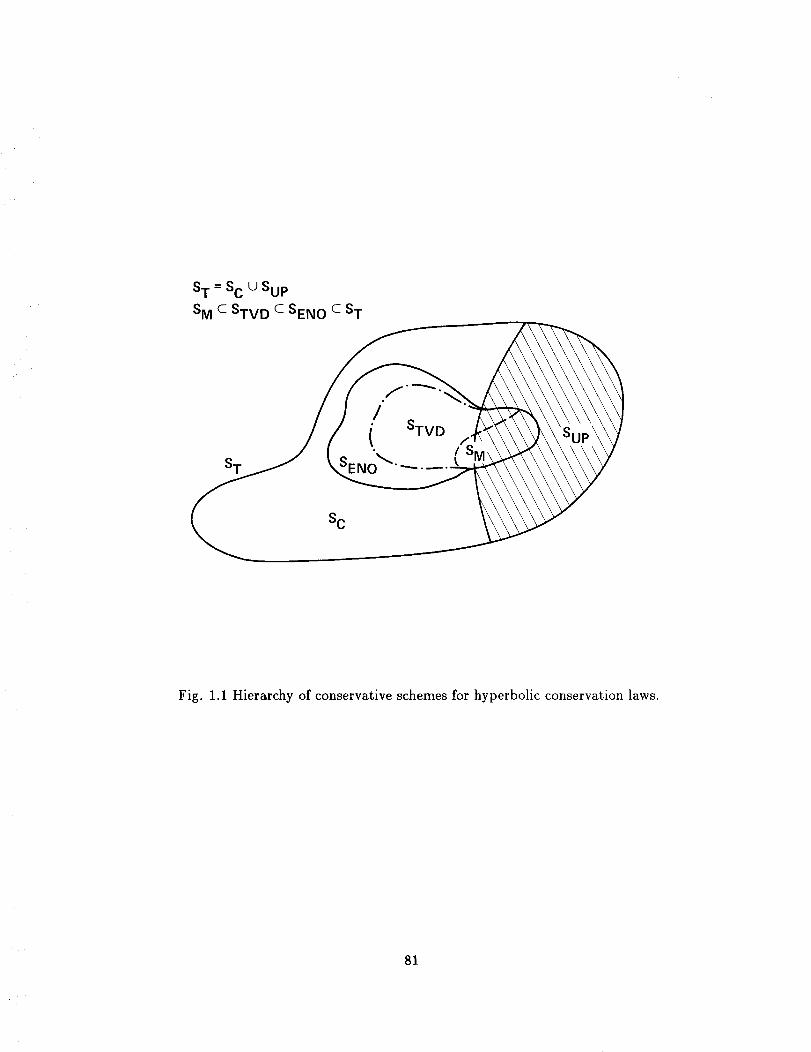
ST = SC u SUp
SM c STV D c SEN O c ST
S "'_ ! SSTJ __
Fig. 1.1 Hierarchy of conservative schemes for hyperbolic conservation laws.
81
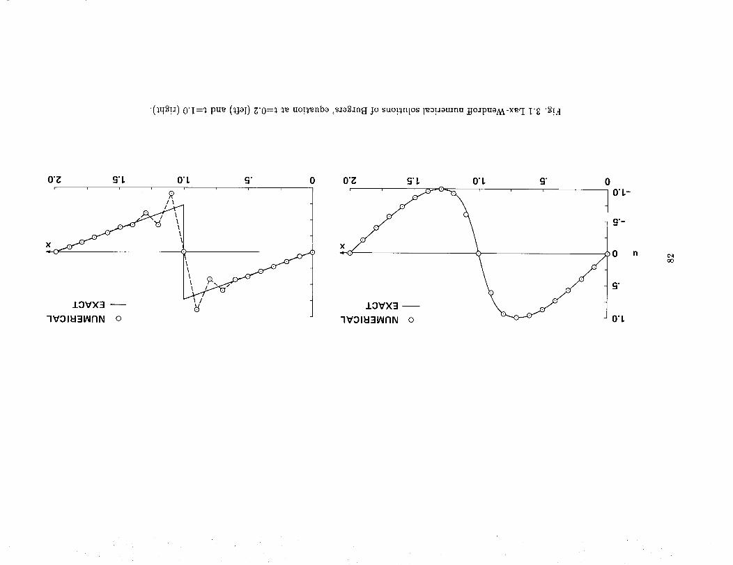
"(_q_!a)O'I_-_pu_(_jot)_'0=__ uo!_nbo ,sao_an_t ]o suo!_nlos l_O!aatunu jjo_puoA_-X_ I I'g "_!_I
0"_ 9"L O'L S" 0, i L
.Lovx3 --
-IVOIU31AInN o
0"_ S'L O'L S"
X , i , i , L t
10V×3 --
._
O'L
n
oo

O'g 9"L O'L _" 0I J J i
-IV::)IU]WnN o
O'g _'L O'L 9" 0
- - - )0 n
oO

(a)
(b)
(c)
O.
r+_l
-1
r÷
r-
r-+r+_l
r-m1
r ÷
0
O(r-, r+) = minmod(1, r-) + minmod(1, r+) - 1
0
r+
r- 1
+r
10
O(r-, r+) = minmod(1, r-, r+)
r-t-
3
2
1
0 v_ 2r +I
0 1 2 30 0
+ 1Q(r-, r+) = minmod(2, 2r-, 2r ,-_-(r- + r+))
r-
r-
r-
Fig. 3.3 Graphical representation of three limiters (3 52,b,c,d).
84

I
0_m
8
I I I I
0 0 0 0
0
!
0
o
°_
o
o
c5It
U
o
o
o
_b.r,,_
85
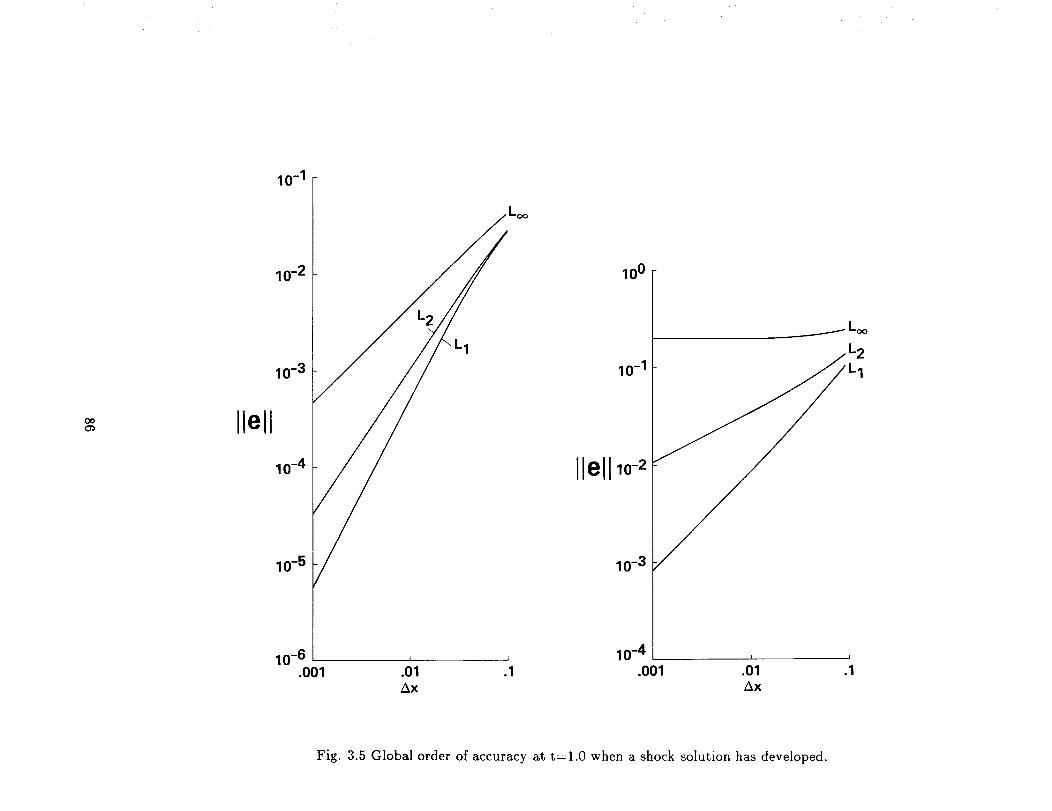
10-1
OOO_ Ilell
10-2
10-3
10-4
10-5
L1
100
10-1
Ilell o
10-3
iLoo
L2
L 1
10-6 , 10 .4.001 .01 .1 .001 .01 .1
Ax Ax
Fig. 3.5 Global order of accuracy at t-1.0 when a shock solution has developed.

L_
o_"
0
_'_
_.g
A
f
9*
t
i , i J
: II i
i -41.4
i i
MACH NUM
i r
\
MACH NUM
MACH NUM,
i __
e.
o)
i! ,i"41-_
U_
"r,_"
i i I
1__ i i
MACH NUM
o _
\
J
MACH NUM
I I I
MACH NUM
!
1J

OoOo
OO
0_
1.3
1.2
0 rD
1.1
1.6-
%4
75O
- iI
25O
O ........ _
1.6
AI
i ®
_i/-=
x
(a)
1.45 4.25 7.05 -6.95 4.15 -1.35 1.45 4.25X
(b)
I ....
• , , , , , .7.05 -6.95 4.15 -135 145 4.25 7,05 -6.95 4.15 -1.35 1.45 4.25 7.05 -6.95 4.15 -1.35 1.45 4.25 7.OS
X X X
(C) (d) (e)
Fig. 4.2 Comparison of the schemes for test case B, for a perfect gas.
(a) Symmetric TVD, non-MUSCL; (b) upwind T\D n(,n-MUS('L, (c) upwind TVD, MUSCL;
(d) van Leer splitting, MUSCL; (e) Steger _nd Warming sphttlng. MUSCL.
Note: (a)-(c) use the identical approximate Riemann solver.
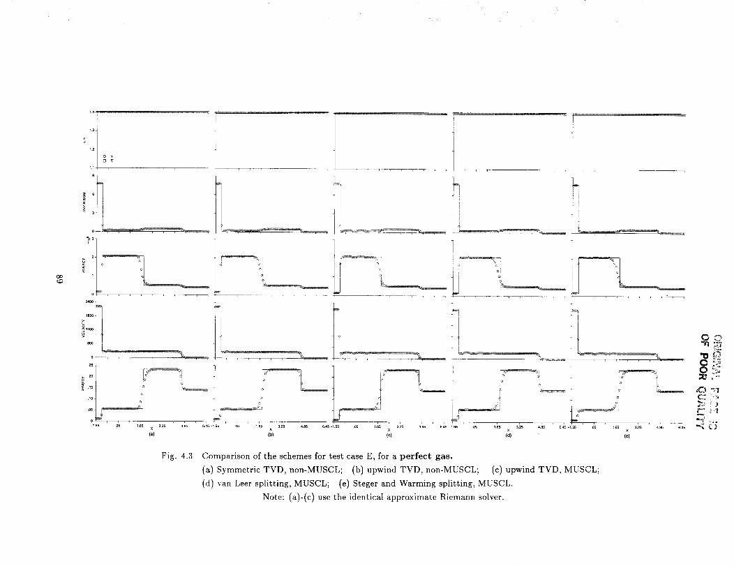
Oo_D
x x x
(a) (b) (c)
0 :>
C: ::'
.05 1.65 3.25 4.85 6.45 -1.55 .05 1.65 3.25 4.85 6.45 i_x X
(d) (e)
Fig. 4.3 Comparison of the schemes for test case E, for a perfect gas.
(a) Symmetric TVD, non-MUSCL; (b) upwind TVD, non-MUSCL; (c) upwind TVD, MUSCL;
(d) van Leer splitting, MUSCL; (e) Steger and Warming splitting, MUSCL.
Note: (a)-(c) use the identical approximate Riemann solver.

¢DO
OO"!1;0
1.o
.5-
g o
l.o
x x x x x
(a) (b) (c) (d) (e)
Fig. 4.4 Comparison of the schemes for test case C, for a perfect gas.
(a) Symmetric TVD, non-MUSCL; (b) upwind TVD, non-MUSCL; (c) upwind TVD, MUSCL;
(d) van Leer splitting, MUSCL; (e) Steger and Warming splitting, MUSCL.
Note: (a)-(c) use the identical approximate Riemann solver.
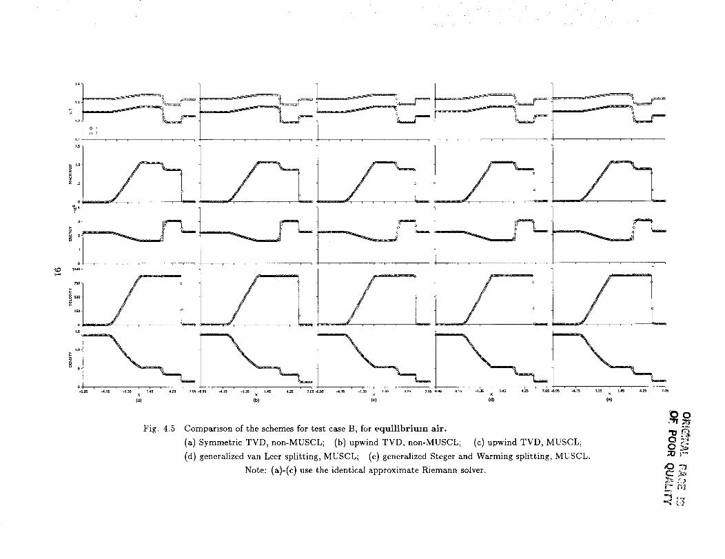
1.3
Fig. 4.5
705 _95 4-415 135 145 425 705 695 _115 135 X 145 425 705-695 415 135 X 145 425 05X
(c) (d) (e)
Comparison of the schemes for test case B, for equilibrium air.
(a) Symmetric TVD, non-MUSCL; (b) upwind TVD, non-MUSCL; (c) upwind TVD, MUSCL;
(d) generalized van Leer splitting, MUSCL; (e) generalized Steger and Warming splitting, MUSCL.
Note: (a)-(c) use the identical approximate Riemann solver.
O"-_

OO
O_
13"
_.2_
0 _
9_
°I
=_ : I
:-_31
_ 4
2400_
1800
i i
"i
i]I
i
• !Iq
°ooI.25 _ -
_1.55 ' .05 1.65 3.25 ' 4.85 6.45 -155 .05 1.65 3.25 4.85 6.45 -_.55 .05 1 65 X 3'25 4.85 6.45-1.55 .05 1.65 3,25 4.85 6.45 -1.55 .05 1.65 3.25 4.85 6,45x x x x
(a) (b) (c) (d) (e)
Fig. 4.6 Comparison of the schemes for test case E, for equilibrium air.
(a) Symmetric TVD, non-MUSCL; (b) upwind TVD, non-MUSCL; (c) upwind TVD, MUSCL;
(d) generalized van Leer splitting, MUSCL, (e) generalized Steger and Warming splitting, MUSCL.
Note: (a)-(c) use the identical approximate Rmmann solver.
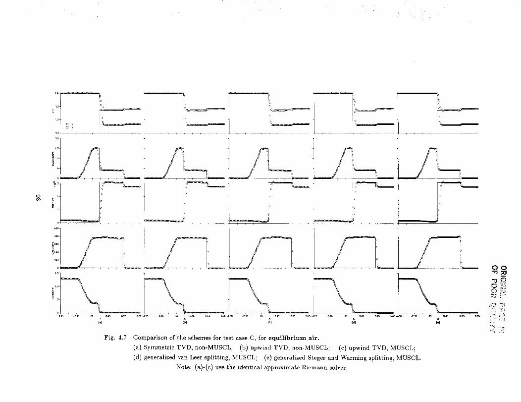
Q ¥ I
20]1,5
1.0
1.o
5
'o ,, , ....
IoIIoL
i
io
o
-4,95 -2.15 .65 3.45 6.25 9.05 4,95 -2,15 .65 3.45 6,25 9._5 _+.95 -2.15 .65 3.45 6.25 6_3 9,¢5 4,95 -2,15x x x
(a) (b) (c)
9.05 _..95 -2+15 .65X
(d)
,,,,,
io
o
c
x
(e)
3.45 s2s 9,es
Fig. 4.7 Comparison of the schemes for test case C, for equilibrium air.
(a} Symmetric TVD, non-MUSCL; (b} upwind TVD, non-MUSCL; (c} upwind TVD, MUSCL;
(d) generalized van Leer splitting, MUSCL; (e) generalized Steger and Warming splitting, MUSCL.
Note: (a}-(c) use the identical approximate Riemann solver.
OO
o3T3_ ......
- , ==
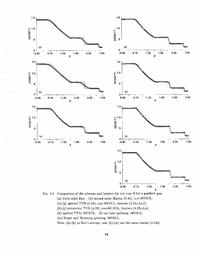
(a)0---- i I i i i i i / i 1
-6.95 -4.15 -1.35 1.45 4.25 7.05X
1.5-
>" 1.0I.-.
zLLI
a.5
1.5 7
O-6.95
(d)
-4)15 _ .3T r _ _ * _-1 5 1.45 4.25 7.05X
1.0"
>,.I,-
z.5-
1.5
0i
-6.95 -4.15i i r I i _ i i 3
-1.35 1.45 4.25 7.05X
1.5-
>- 1.0I--
zuJ
.5
(e)0 i I i I i i i I
-6.95 -4.15 -1.35 4.25 7.05I I
1.45X
>- 1.0I--
ZUJ
E3.5
(c) -'=="""-"_
-6.95 -4.15 -1. 5 1.45 4.25 7 5X
1.5-
>. 1.0I-
zLM
.5-
(f)o-6.95
I I i _ t I-41 425X
Fig. 4.8
1.5-
I-"
III
a .5
(g)0 I I I I I I --7 F 1
-6.95 -4.15 -1.35 1.45 4.25X
Comparison of the schemes and limiters for test case B for a perfect gas.
(a) First-order Roe; (b) second-order Harten (3.45), non-MUSCL;
(c)-(g) upwind TVD (4.34), non-MUSCL, limiters (4.34c,d,e,f);
(h)-(j) symmetric TVD (4.33), non-MUSCL, limiters (4.33c,d,e);
(k) upwind TVD, MUSCL; (1) van Leer splitting, MUSCL;
(m) Steger and Warming splitting, MUSCL.
Note: (a)-(k) us Roe's average, and (k)-(m) use the same limiter (4.34e).
I
7.05
94

R_t_ _ _2 _ _ :'"!'% .........
_,_ _i_ _ : '_ i_ !_ : :_'_
1.5-
1°5-
I 1 I I T--
1.45 4.25X
>- 1.0
Z
.5-
(i)0-6.95
l I l ) i r _ i i
-4.15 -1.35 1.45 4.25 7.05X
i T I i m i l I [-4 15 -1.35 1.45 4.25 7.05X
1.5
1.0
Z
_.5
0-6.95
1 i i i I i i i i I
-4.15 -1.35 1.45 4.25 7.05X
1.5-
1.0I--
ZW
a .5
i l i i i i i i i i
-6.95 -4.15 -1.35 1.45 4.25 7.05X
1,5-
>- 1.0I.-
ZILl
.5-
.'I5 ' 3" E , , , ' 7.'05-4 -1. 5 1.45 4.250-6.95
X
Fig. 4.8 (Concluded)
95
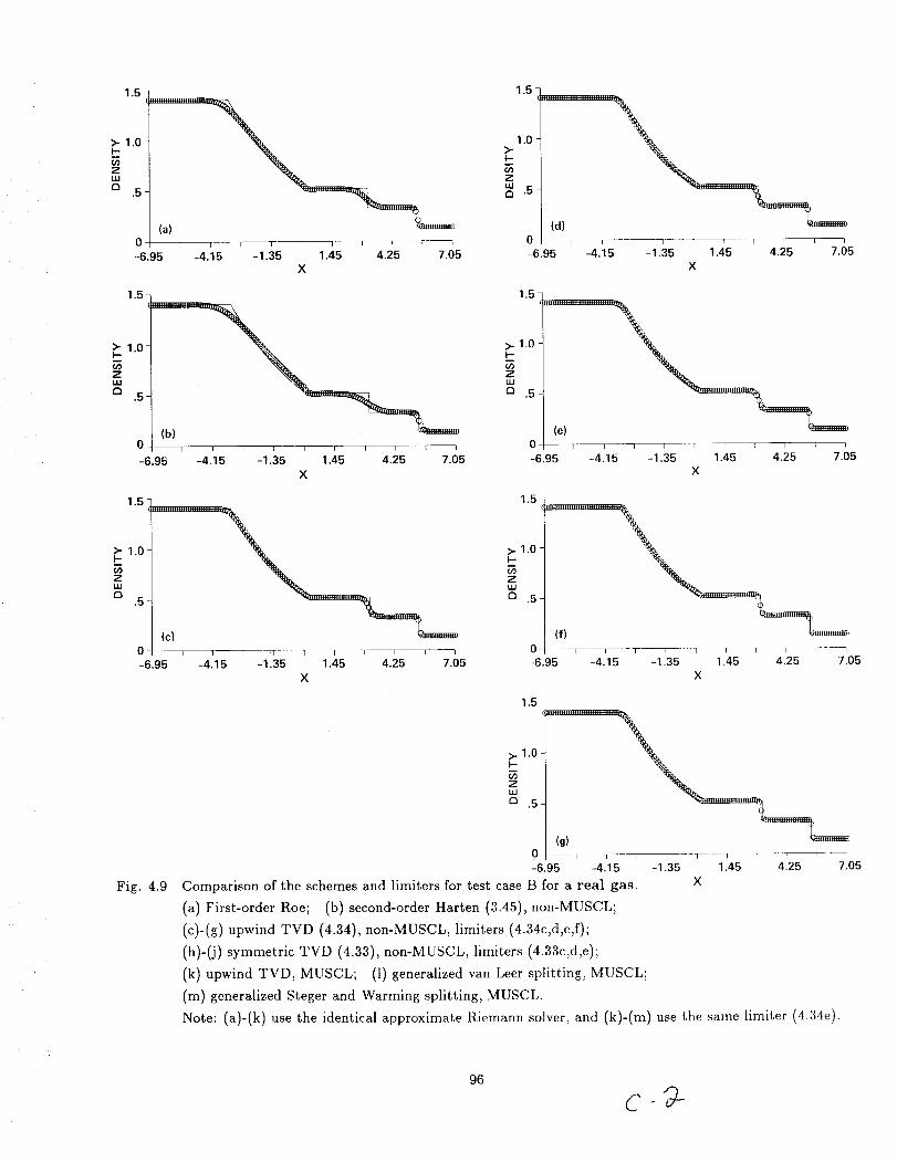
1.5
>" 1.0I--
ZILl
a.5
I i
-6.95 -4.15 -1.35
::::::::::::::::::::::::::; =_
(a)
1.45 4.25 7.05
X
1.5
1.0>-I-
Z
_.5
(d)0
-6.95 -4.15 -1.35 1.45 4.25 7.05
X
1,5-
>- 1.0I..-
ZLU
a.5-
I
-6.95 -4.15
I I t I t I I I I
-1.35 1.45 4.25 7.05
X
1.5-
>. 1.0I-
ZLU
a .5
i
-6.95 -4Jl 5
(e)
-1.35 1.45 4.25 7.05
1.5
>- 1.0 ................................
u.I
a.5
I =r
(c)0 i i
-6.95 -4.15 -1.35I I i I i /
1.45 4.25 7.05
X
1.5
>- 1.0I--
ZLU
a .5
-6.95 -4)15 -1.35 1.45 4.25 7.05
X
Fig. 4.9
1.5
>',,,>,1-_1"0 -_""""_.5_
(g)
0 .... --F , • .T2 _ i-6.95 -4.15 -1.35 1.45 4 5 7 05
Comparison of the schemes and limiters for test case B for a real gas. X
(a) First-order Roe; (b) second-order Harten (3.45), non-MUSCL;
(c)-(g) upwind TVD (4.34), non-MUSCL, limiters (4.34c,d,e,f);
(h)-(j) symmetric TVD (4.33), non-MUSCL, limiters (4.33c,d,e);
(k) upwind TVD, MUSCL; (1) generalized van Leer splitting, MUSCL;
(m) generalized Steger and Warming splitting, MUSCL.
Note: (a)-(k) use the identical approximate Riemann solver, and (k)-(m) use the same limiter (4.34e).
96
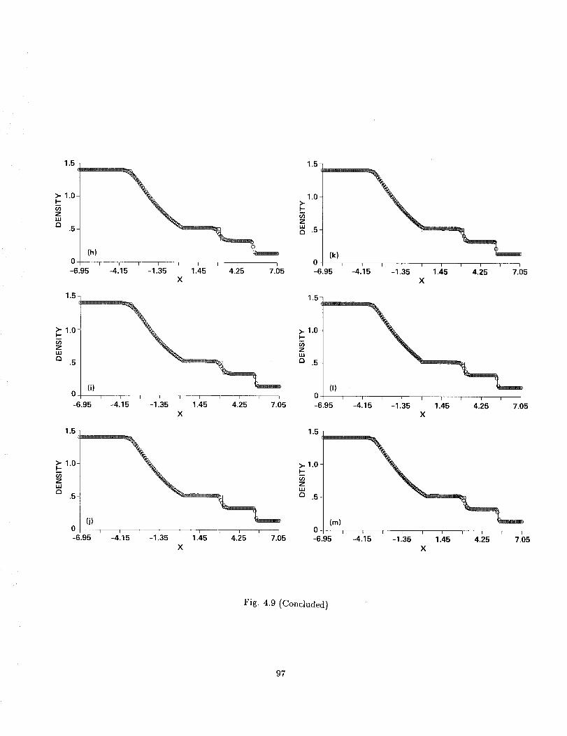
1.5-
>- 1.0I-
ZuJC]
.5-
I
-6.95 -4.'15 -1.35
(h)
I I ] I I I I I
1.45 4.25 7.05X
>-I--O3
1.5
1.0
.'I5 ' ' ' ' ' ' ' 'i4 -1.35 1.45 4.25 7.05
Z_.5
0-6.95
1.5-
>- 1.0 _I-
ZLU
.5-
0-
-6.95
(i)T T I I I I i I I I
-4.15 -1.35 1.45 4.25 7.05X
(I)0-6.95
I i I I I I i [ I
-4.15 -1.35 1.45 4.25 7.05X
1.5_.............................. 15=
_ -O3
UJ
a .5jj (J) _ ........................ _ .5-
O. , , , , , , _ , , , 0-6.95 -4.15 -1.35 4.25 7.051.45
X
(m)
-6.95
::::::::::::: :: :::::::::::::::.-_
-41 35 ;, ....5 -1 1 5 425 705X
Fig. 4.9 (Concluded)
97
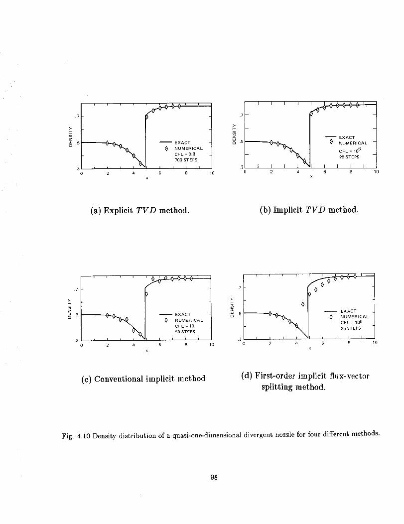
.7
>-
Z
W .5_m,
.3
2 4
-- EXACT
{} NUMERICAL
CFL = 0.8
700 STEPS
6 8
×
10
.7
.5_
r 1 T T
I -I "7- _x_cm,_._,_I _ NUMER,OAL-
'"% I CFL:,O'_%,1 _STE_S
2 4 6 8 10
x
(a) Explicit TVD method. (b) Implicit TVD method.
.7
>.
Z
w .5£3
r T 1
2 4
-- EXACT
<) NUMERICAL
CFL = 10
50 STEI_S
6 8
x
10
>..l-
Z
W .5,"7
_,.rI -- EXACT
v _ I <) NUMERICAL
I c_=1o6I
.____t _ _ [ 1 1_--
2 4 6 8 10
x
(c) Conventional implicit method (d) First-order implicit flux-vector
splitting method.
Fig. 4.10 Density distribution of a quasi-one-dimensional divergent nozzle for four different methods.
98
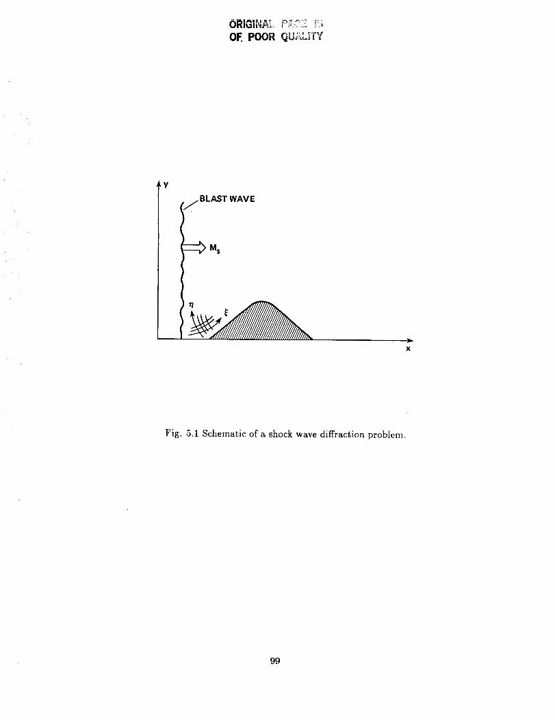
- '° _,_,._:, !!!iORIG|NA__ '_ '_OE POOR QU_-,_n_
/ BLAST WAVE
X
Fig. 5.1 Schematic of a shock wave diffraction problem.
99

2.0
1.5
Y1.0
.5
0-1.0 -.5 0 .5
X1.0
Fig. 5.2 The 317 × 100 orthogonal grid.
100
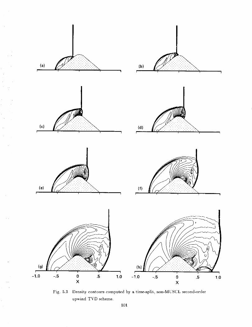
(a) _ __ (b)I I I I
(c) _ _ (d)
I L I
, (e) _, , (f) , ,
, (g) , ,'(h)
-1.0 -.5 0 .5 1.0 -1.0 -.5 0 .5 1.0
X X
Fig. 5.3 Density contours computed by a time-split, non-MUSCL second-order
upwind TVD scheme.
101
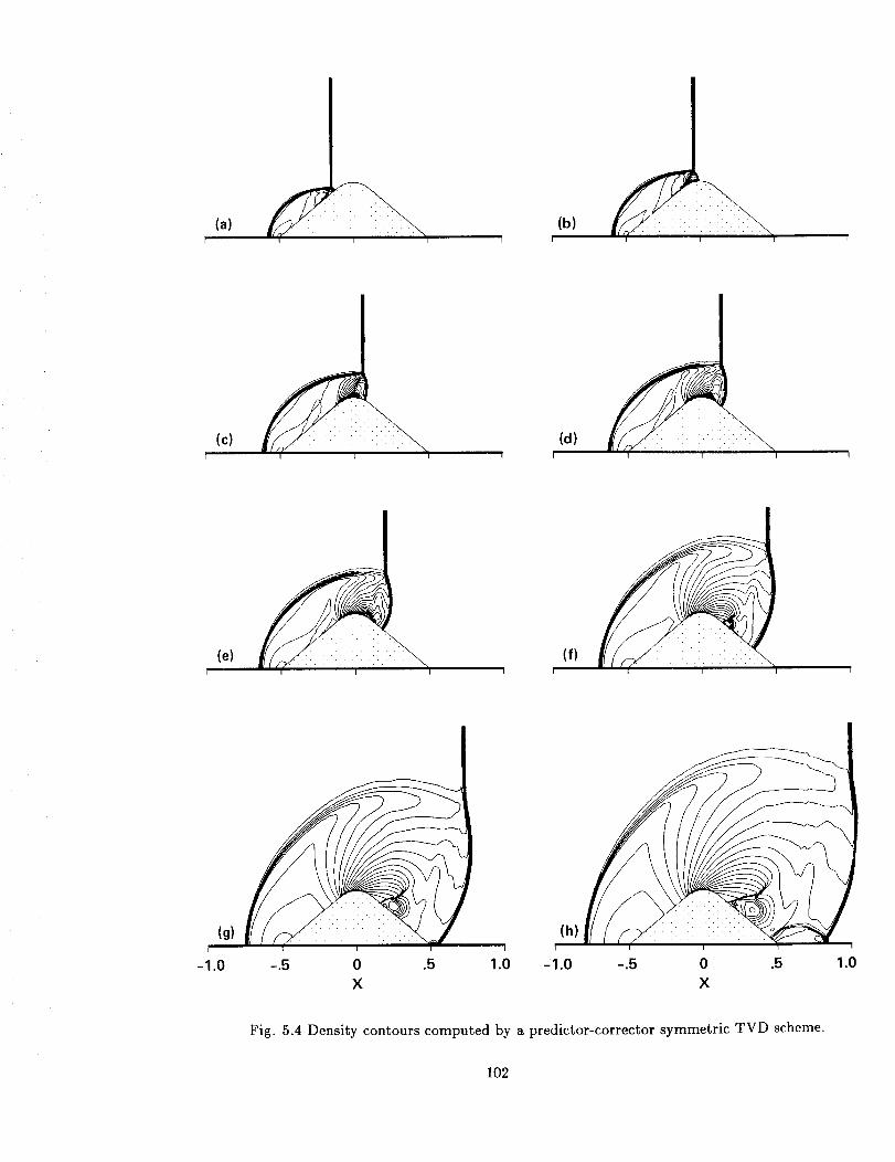
(a) _ (b)I I I
I I I
, (e) _(f)
, (g)]
-1.0 -.5 0 .5 1.0 -1.0 -.5 0 .5 1.0
X X
Fig. 5.4 Density contours computed by a predictor-corrector symmetric TVD scheme.
102

, (a)
(c) , d
-1.0 -.5 0 .5 1.0 -1.0 -.5 0 .5 1.0X X
Fig. 5.5 Comparison of density contour plots from different TVD schemes.
(a) Predictor-corrector symmetric TVD with limiter (4.33c);
(b) predictor-corrector symmetric TVD with limiter (4.33d);
(c) predictor-corrector symmetric TVD with limiter (4.33e);
(d) time-split second-order upwind TVD, non-MUSCL with limiter (4.34d,f)
103
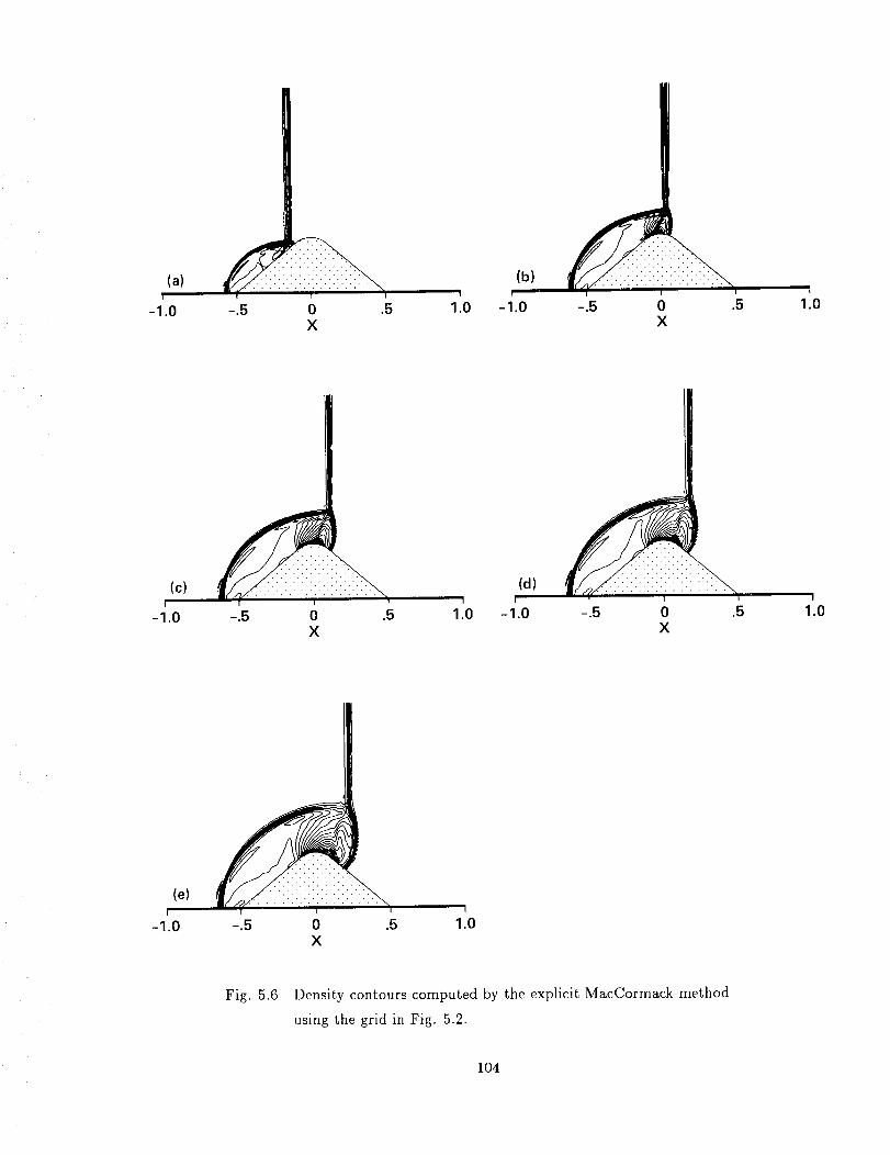
(a)I
-1.0 -.5 0 .5X
I
1.0
(b) ............
-1.0 -.5 0X
.5 1.0
(c)I
-1.0I
-.5 0 .5X
I
1.0
,(d) _,.
-1.0 -.5 0 .5X
I
1.0
-1.0 -.5 0 .5X
I
1.0
Fig. 5.6 Density contours computed by the explicit MacCormack method
using the grid in Fig. 5.2.
104
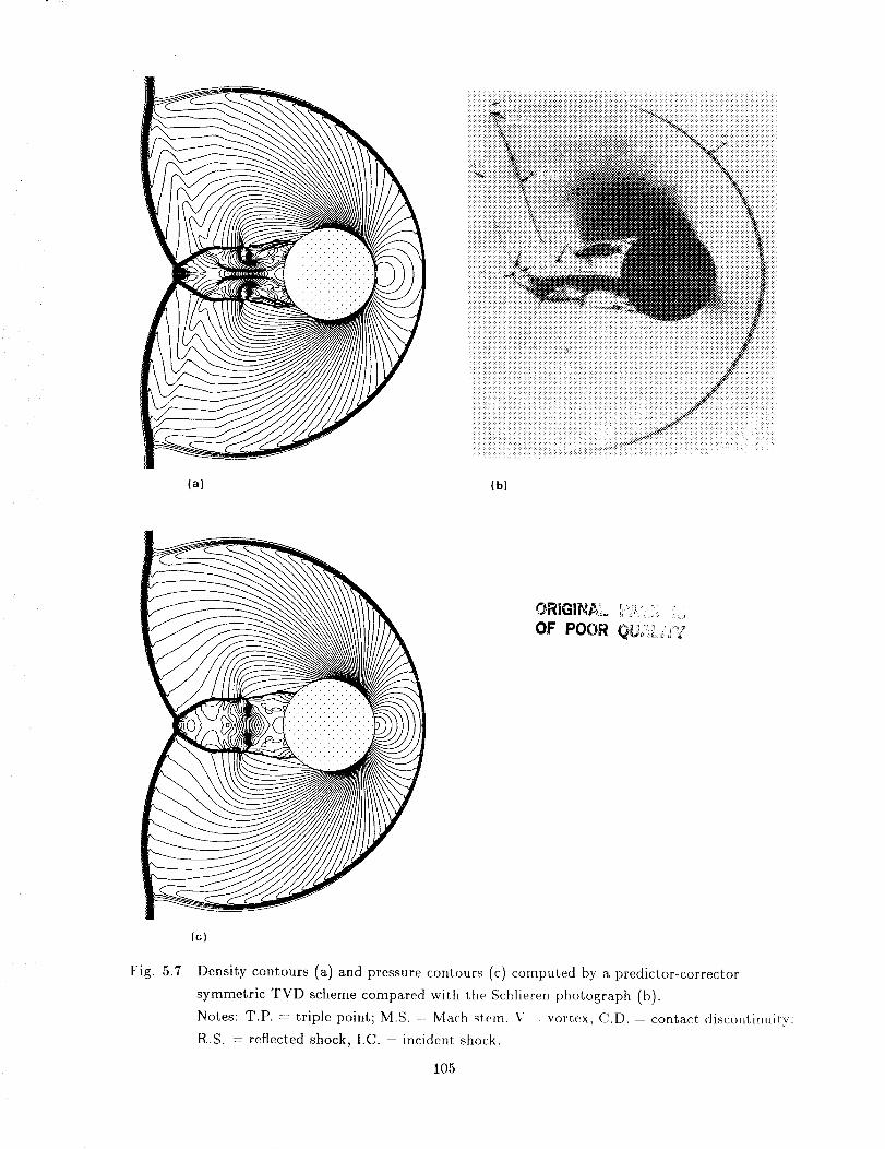
(a) (b)
ORIGINS'.: _'_',.....
OF POOR QU;'_;'2_;_
Fig. 5.7
(c)
Density contours (a) and pressure cont_ours (c) computed by a predici_or-corrector
symmetric TVD scheme compared with the Schlieren photograph (b).
Notes: T.P. = triple point; M.S. --- Math _tmn, V _ vortex, C.D. - contact discontinuity:
RS. = reflected shock, I.C. = incident shock.
105

SHOCK TUBE\
-- °
INCIDENT ----
SHOCK
[_Ms
\\
\
\ \\\ \\ \\\ \
= 2 I _ = 30°
II I/
/ /// /
/ //.._JJ /
/ // /
f (
\ \\ \
\ \\ \
\ \\ \
Y A
/ // /
/ // /
//
(
PLEXI-GLASS j
Fig. 5.8 Schematic of the experiment.
Y
TIMAGE PLANE
\\\\\,,,_Jk_],,,,,,,,. .........WALL BOUNDARY
INFLOW _ IBOUNDARY [_ M s = 2
OUTFLOW BOUNDARY /
PLANE OF SYMMETRY/ _
IMAGE PLANE fX
Fig. 5.9 Schematic of the shock tube computational domain (Cartesian grid).
106

\\
\\ OUTER BOUNDARY
OF C-GRID
\\\
III
//
/CURVEDSHOCK
I/
/OUTEROF CARTESIAN
GRID
Fig. 5.10 Schematic of the computational domain (curved incident shock).
107

QUALITY
/ i
Fig. 5.11 Density contours computed by the time-split upwind TVD scheme (4.34a,c,f)
compared with interferograms at approximately the same time instants.
108
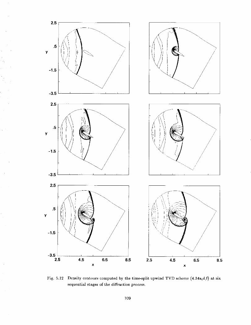
Fig. 5.12 Densitycontourscomputedbythetime-splitupwindTVD scheme(4.34a,d,f)at sixsequentialstagesofthediffractionprocess.
109
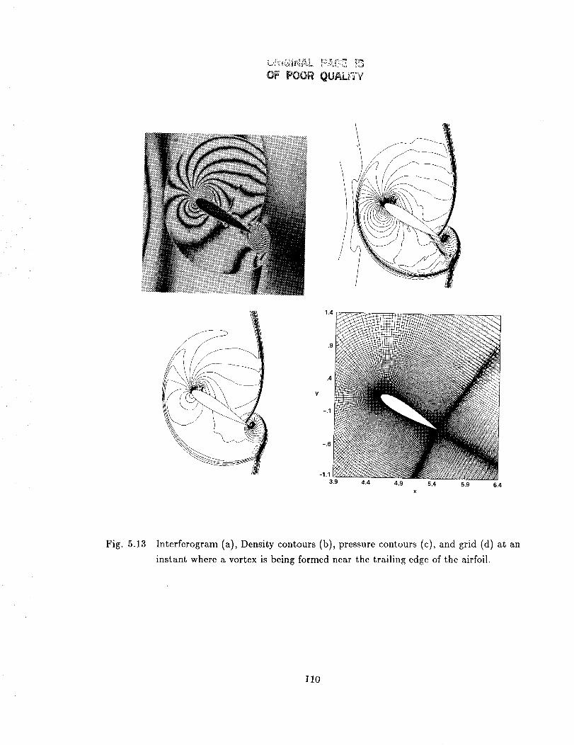
•i_ ¸_, _,:,,_:_ _
OF POOR QUALITY
//
Fig. 5.13 Interferogram (a), Density contours (b), pressure contours (c), and grid (d) at an
instant where a vortex is being formed near the trailing edge of the airfoil.
110

Y
lx
[_M s = 1.5
BODY WAKE CUT
OUTER BOUNDARY
BOUNDARY
Fig. 5.14 Schematic of the computational domain (planar incident shock ).
111

iiiii
t
Fig. 5.15 Density contours computed by the time-split upwind TVD scheme (4.34a,d,f) using a
curved shock (middle) and a planar shock (right) compared with the interferograms
at approximately the same time instants.
112
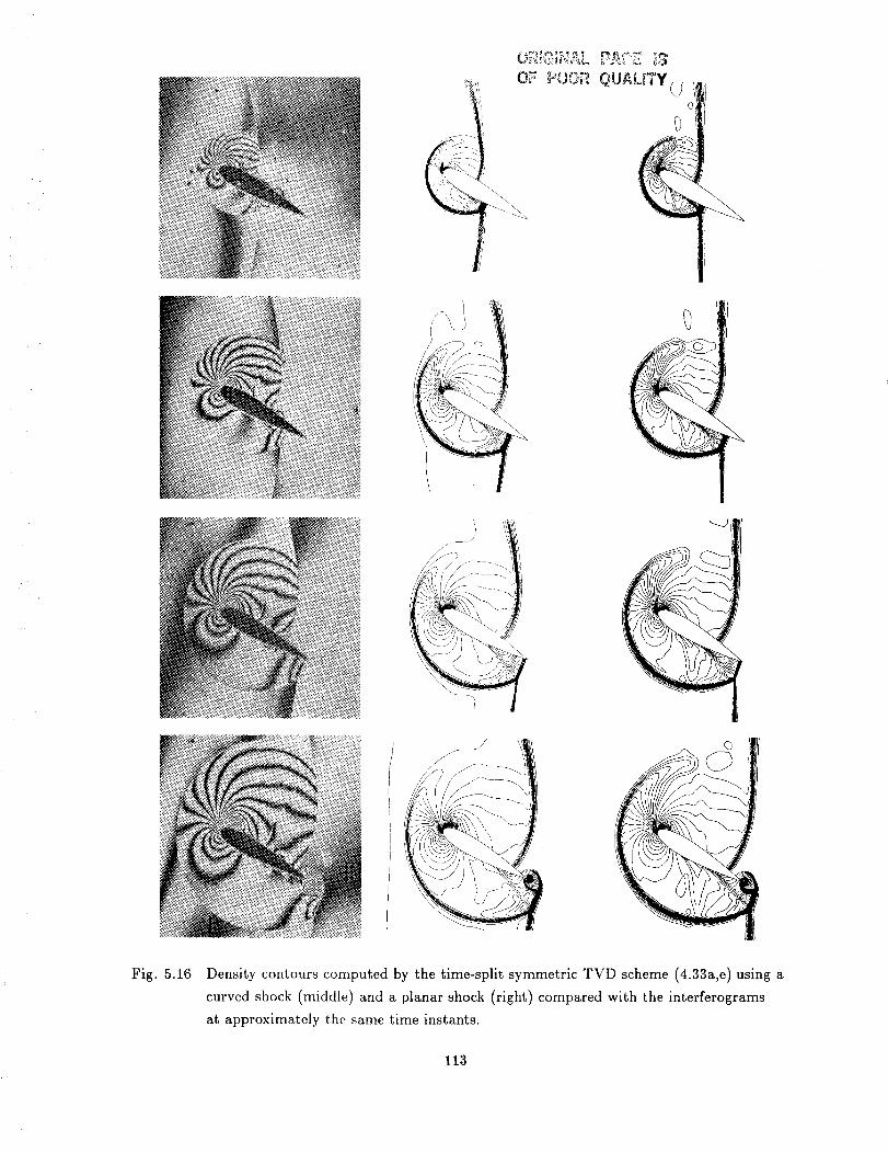
Fig. 5.16 Density contours computed by the time-split symmetric TVD scheme (4.33a,e) using a
curved shock (middle) and a planar shock (right) compared with the interferograms
at approximately the same time instants.
113
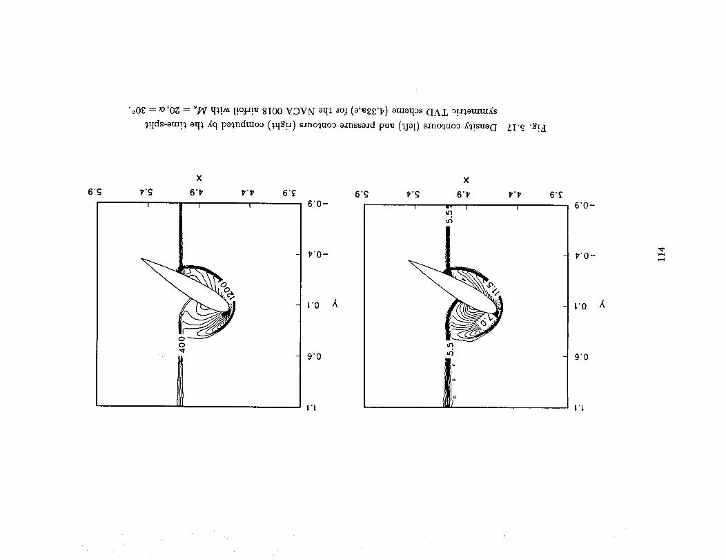
"o0_ = _°'0_ = s/4/q_t._ [!oja[._ 8100 VDVIq oq_ aoj (o'_¢_'17) ouloq_s (IA,I, _!_otutu,(s
_!lds-otut._ oq_ _q po_ndu, o_ (_q_!a) s_no_uo_ o_nsso_d pu_ (_jo[) s_no_uo_ _!suo([ I LI'_ "_t.A
6"_
0
'_'0--
l'0 A
- 9"0
i'|
¢i
6"£
6"0-
t'O
9"0
t'L
,(
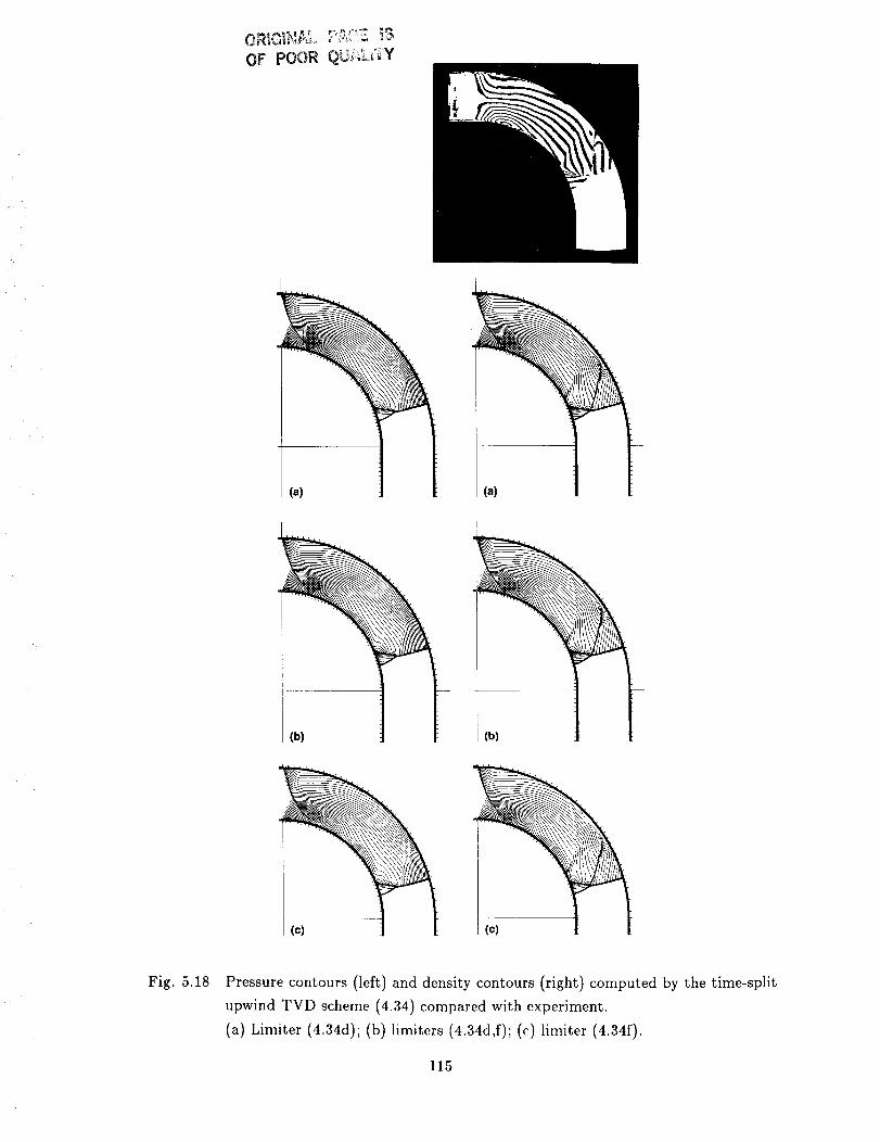
OF POOR Q_",_.__Y
(a)
(b) (b)
(c) (c)
Fig. 5.18 Pressure contours (left) and density contours (right) computed by the time-split
upwind TVD scheme (4.34) compared with experiment.
(a) Limiter {4.34d); (b)limiters (4.34d,f); (c)limiter (4.34f).
115
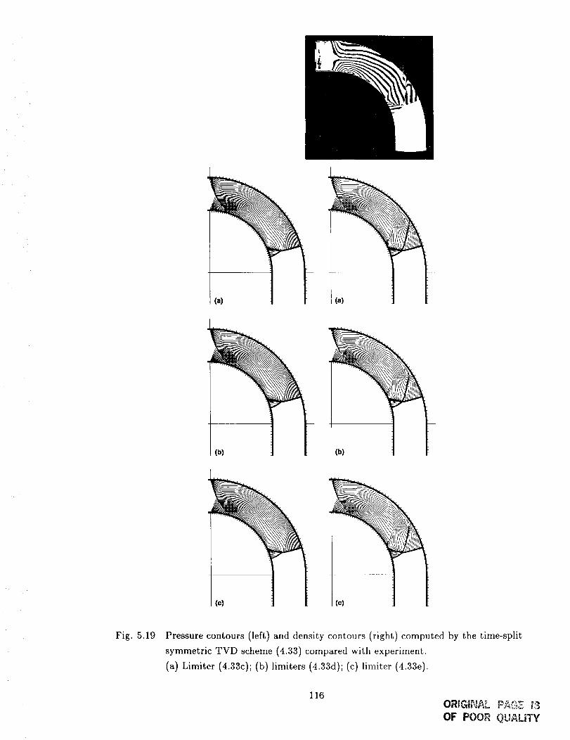
(a)
(b)
(c)
(a)
Fig. 5.19 Pressure contours (left) and density contours (right) computed by the time-split
symmetric TVD scheme (4.33) compared with experiment.
(a) Limiter (4.33c); (b)limiters (4.33d); (c)limiter (4.33e).
116
OF POOR QL)ALiTY
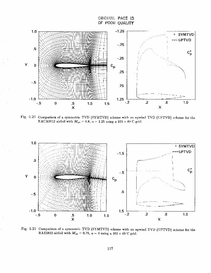
OR,_j,J;_,_. PAGE 13
OF POOR QUgLiTY
1.0
.5
Y 0
-.5
-1.25
-.75
-.25
Cp
.25
.75
+ SYMTVD
--- UPTVD
I,
hJ
!,
.2-1.0 1.25 -- :_-_"
-.5 0 .5 1.0 1.5 -.2 .6 1.0X X
Cp
Fig. 5.20 Comparison of a symmetric TVD (SYMTVD) scheme with an upwind TVD (UPTVD) scheme for the
NACA0012 airfoil with Moo = 0.8, a = 1.25 using a 163 × 49 C grid.
Y
1.0
.5
-.5
-1.5
-.5
Cp
f .......... .!
+ SYMTVD
---UPTVD
*
! Cp
i •
?
1.5-,2
-1.0-.5 0 .5 1.0 1.5 .2 .6 1.0
X X
Fig. 5.21 Comparison of a symmetric TVD (SYMTVD) scheme with an upwind TVD (UPTVD) scheme for the
RAE2822 airfoil with Moo = 0.75, a = 3 using a 163 × 49 C grid.
117

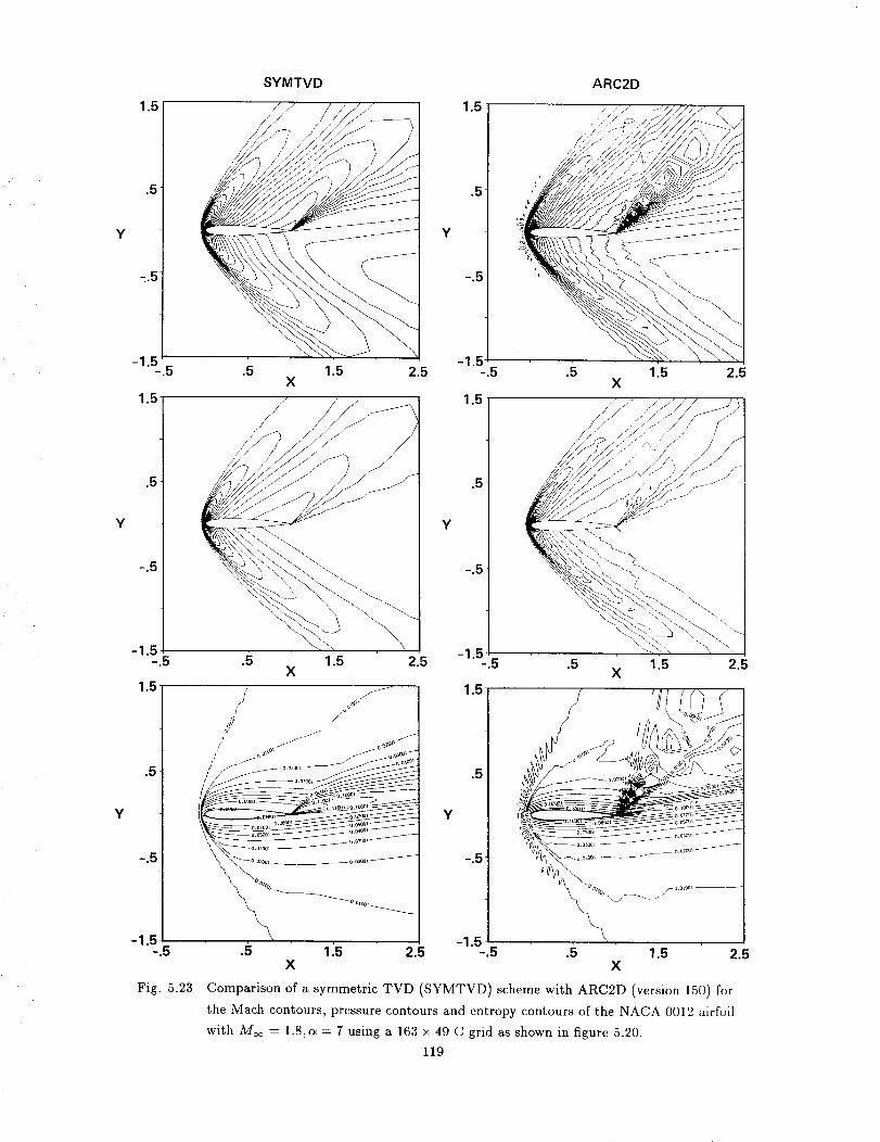
SYMTVD ARC2D
1.5 _ 1.5 -r _/ /7-/7777---7--
-'c _./ " /. .5I@5
_'.______ 4
-1"5.5 .5 ' \"1_:5 ' 2.5 -1"5.5 .5 ' 1_"5' " 2.5X X
1.5 f /-J 1.5-f
/? _ o._,_
\N_--_ ...... _Z_, _\_--°_,___ _-._ \_,______ ...._ _._
ea%_
-.5 .5 1.5 2.5 -.5 .5 1.5 2.5X X
Fig. 5.23 Comparison of a symmetric TVD (SYMTVD) scheme with ARC2D (version 150) for
the Mach contours, pressure contours and entropy contours of the NACA 0012 airfoil
with M_ = 1.8, a = 7 using a 163 x 49 C grid as shown in figure 5.20.
119

GRID PRESSURE COEFFICIENT
Y 0
0 .5 1.0 1.5
X
-1.5
!
Cp I
.5
+ EXPERIMENT,
**+ COOK et al., 1979
_ COMPUTED
C* -
+, p
+ ?" ,4+
*,. - .4%
_' -±t %+ .+ _+,
i
1.5__
-.2 .2 .6 1.0
X
Y 0
-.5
/
\\
MACH NUMBER CONTOURS
/ /
I ; /
\
/
/
'1
-1
1.0
.5
Y 0
-.5
/
J
/
//
110 1.5
-1.0 -1.0
-.5 0 .5 -.5 0
PRESSURE CONTOURS
.5 li0 1.5
X
Fig. 5.24 A thin layer Navier-Stokes calculation for the RAE2822 airfoil using an upwind
TVD scheme with a 249 x 51 O grid, Moo -- 0.73,c_ -- 2.79, Re -- 6.5 x 10⁶.
120
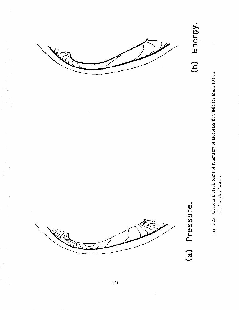
\
\
>,(:nL_-
(1)e-
W
A
t_
CO(D
(1)t_
12.
O
O
t._
O
O
_9
O
_D
O
O
hO
0
0
_S
_b
121
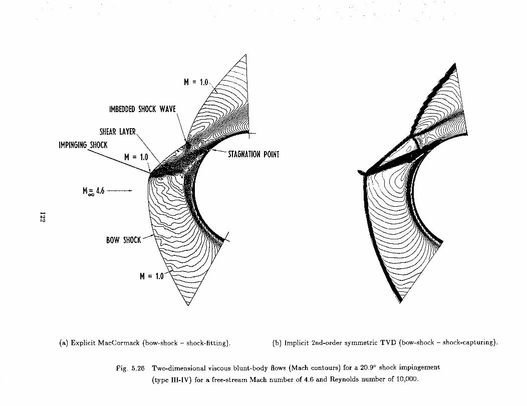
M = 1.0,,
IMBEDDEDSHOCKWAVE
SHEAR
IMPINGINGSHOCK
M__- STAGNATIONPOINT
t==_
M_o4.6 --
BOW
(a) Explicit MacCormack (bow-shock - shock-fitting). (b) Implicit 2nd-order symmetric TVD (bow-shock - shock-capturing).
Fig. 5.26 Two-dimensional viscous blunt-body flows (Mach contours) for a 20.9 ° shock impingement
(type III-IV) for a free-stream Mach number of 4.6 and Reynolds number of 10,000.

2
Y
Fig. 5.27 Density contours of Mach 25 for a real gas computed by
a second-order upwind TVD scheme.

p = 1 atmT = 1200 KM=4
Z
__o _Z = 0.29 cm/
X
._---1 cm _ _ 2 cm
Fig. 6.1 Geometry and inflow condition.
124
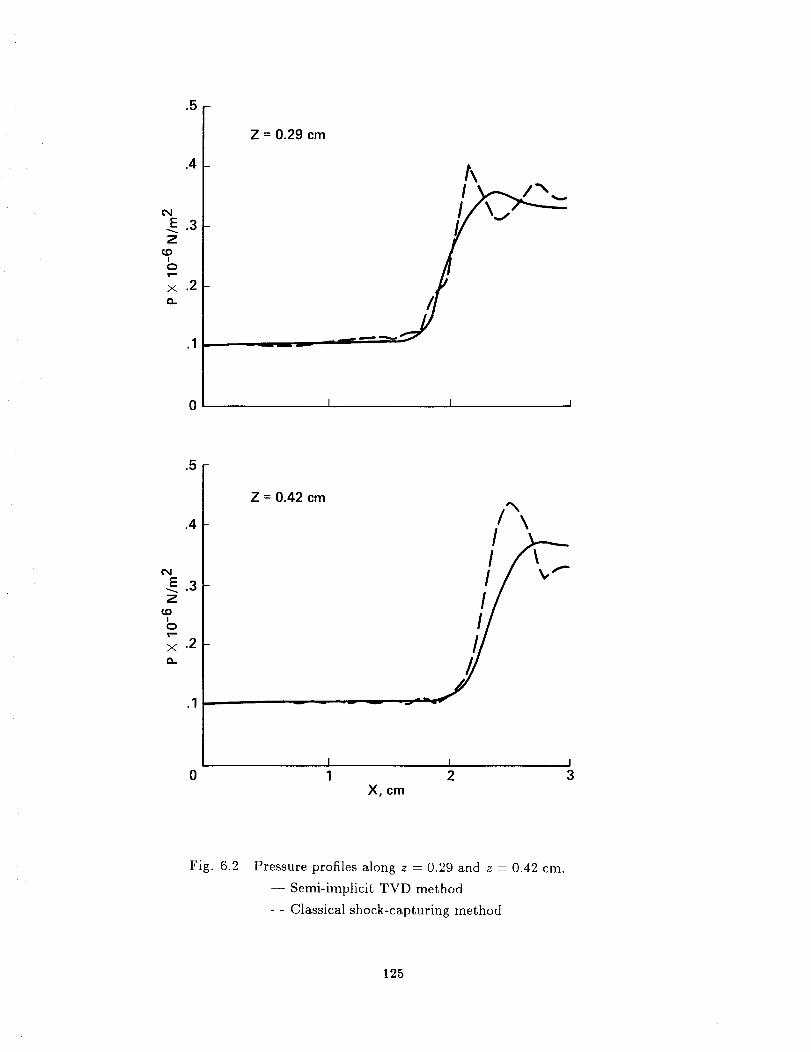
.5
.4
N
E.3Z
t.OI
Q
X .2
.1
Z -- 0.29 cm
h
J
I I J
.5
.4
¢N
E.3Z
I
× .2o_
.1
[ Z = 0.42 cm,%
/ \
j//I I I
0 1 2 3X, cm
Fig. 6.2 Pressure profiles along z = 0.29 and z = 0.42 cm.
-- Semi-implicit TVD method
- - Classical shock-capturing method
125
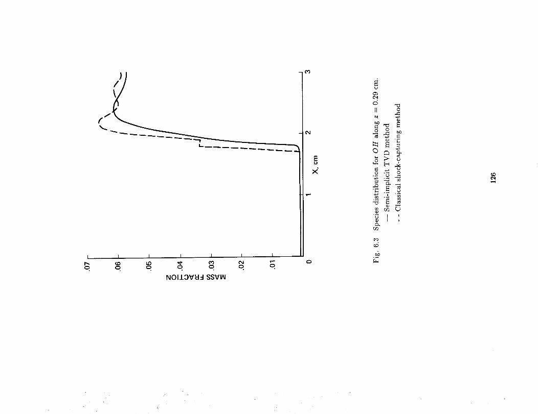
/
I I I
I_ t,,.o 1.0
I °
I I
0 0
NOIJ_3VEI.-I SSVIAI
I
0
-cO
E
x"
I
0
II o
o• _
_'_ _
_1 :
_D
bb
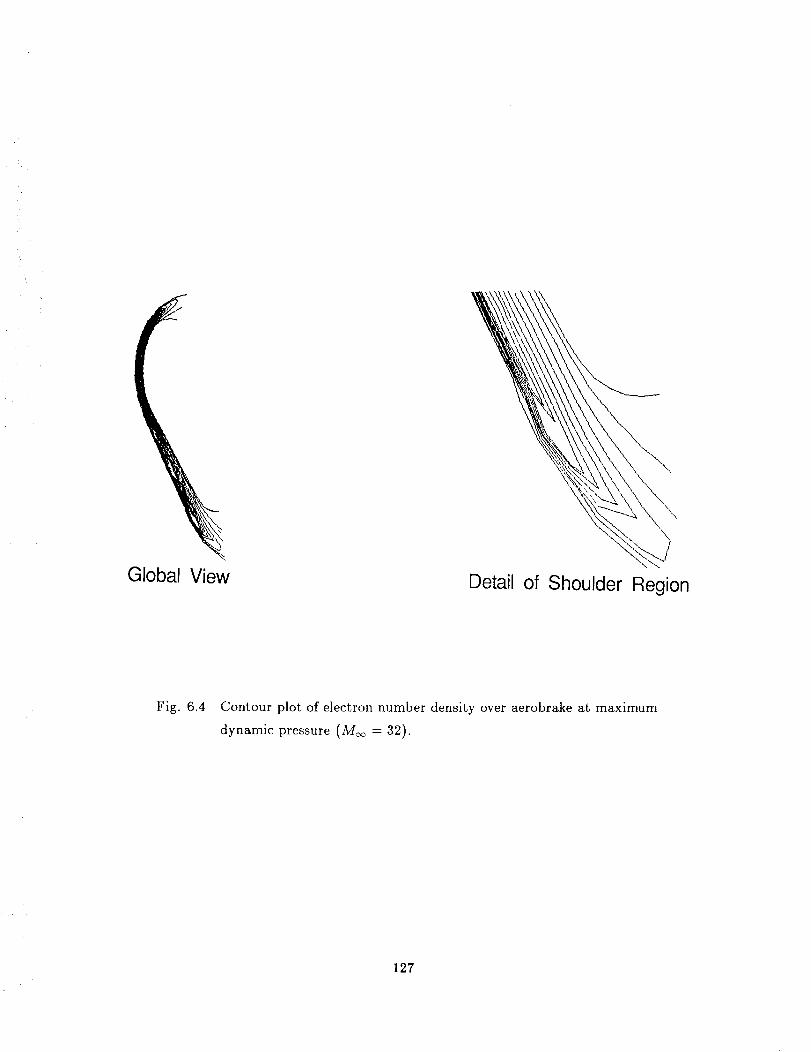
Global ViewDetail of Shoulder Region
Fig. 6.4 Contour plot of electron number density over aerobrake at maximum
dynamic pressure (Moo -- 32).
127
Report Documentation PageNat_',al Aeror_Jl_cs and
SLI,_ r/kdmlr_sIral_'_l
1. Report No.
NASA TM-89464
4. Title and Subtitle
2. Government Accession No.
Upwind and Symmetric Shock-Capturing Schemes
7. Author(s)
3. Recipient's Catalog No.
5. Report Date
May 1987
H. C. Yee
9. Performing Organization Name and Address
Ames Research Center
Moffett Field, CA 94035
12. Sponsoring Agency Name and Addre_
National Aeronautics and Space Administration
Washington, DC 20546
6. Performing Organization Code
8. Performing Organization Report No.
A-87236
10. Work Unit No.
505-60
11. Contract or Grant No.
13. Type of Report and Period Covered
Technical Memorandum
14. Sponsoring Agency Code
15o Supplementary Notes
Point of Contact: H. C. Yee, Ames Research Center, M/S 202A-I
Moffett Field, CA 94035 (415) 694-4769 or FTS 464-4769
16. Abstract
The development of numerical methods for hyperbolic conservation laws has
been a rapidly growing area for the last ten years. Many of the fundamental
concepts and state-of-the-art developments can only be found inmeeting pro-
ceedings or internal reports. This review paper attempts to give an overview
and a unified formulation of a class of shock-capturing methods. Special
emphasis will be on the construction of the basic nonlinear scalar second-
order schemes and the methods of extending these nonlinear scalar schemes to
nonlinear systems via the exact Riemann solver, approximate Riemann solvers
and flux-vector splitting approaches. Generalization of these methods to
efficiently include real gases and large systems of nonequilibrium flows will
be discussed. The performance of some of these schemes is illustrated by
numerical examples for one-, two- and three-dimensional gas dynamics problems.
17. Key Words(SuggestedbyAuthor(s)) Numerical method,
Finite difference method, Computational
fluid dynamics, System of hyperbolic
conservation laws, Stiff problems, Shocl
capturing, Conservative differencing,
TVD schemes, Implicit methods
18. Distribution Statement
Unclassified-Unlimited
Subject Category - 64
19. Security Classif. (of this report)
Unclassified
IASA FORM 1626 OCT 86
20. Security Classif. (of this page)
Unclassified
21. No. of pages _. Price
127 AO7
GPO 788-003/T 9176

![Central-Upwind Schemes for Two-Layer Shallow Water Equationsgpetrova/KP_2l.pdf · Central-Upwind Schemes for Two-Layer Shallow Water ... we refer the reader to [2], ... Central-Upwind](https://img.pdfslide.us/doc/110x75/5abcf7377f8b9a24028e74bf/central-upwind-schemes-for-two-layer-shallow-water-gpetrovakp2lpdfcentral-upwind.jpg)


![Upwind compact finite difference scheme for time-accurate …lsec.cc.ac.cn/~lyuan/2010amc.pdf · 2010. 2. 25. · The upwind compact scheme developed in [37] combined Fu and Ma’s](https://img.pdfslide.us/doc/110x75/60a974aa58708c682610ca82/upwind-compact-finite-difference-scheme-for-time-accurate-lsecccaccnlyuan.jpg)