lable at ScienceDirect

Journal of Cleaner Production 183 (2018) 1110e1121

Contents lists avai

Journal of Cleaner Production

journal homepage: www.elsevier .com/locate/ jc lepro

A high temporal-spatial resolution air pollutant emission inventory foragricultural machinery in China

Jianlei Lang a, *, Jingjing Tian a, Ying Zhou a, **, Kanghong Li a, Dongsheng Chen a,Qing Huang b, Xiaofan Xing a, Yanyun Zhang a, Shuiyuan Cheng a

a Key Laboratory of Beijing on Regional Air Pollution Control, College of Environmental & Energy Engineering, Beijing University of Technology, Beijing,100124, Chinab School of Environment, Jinan University, Guangzhou, 510632, China

a r t i c l e i n f o

Article history:Received 10 August 2017Received in revised form8 January 2018Accepted 12 February 2018Available online 22 February 2018

Keywords:Agricultural machinery emissionsChinaCounty-levelSpatial distributionTemporal distribution

* Corresponding author. College of EnvironmentalLaboratory of Beijing on Regional Air Pollution Contronology, Beijing, 100124, China.** Corresponding author.

E-mail addresses: jllang@bjut.edu.cn (J. Lang), y.zh

https://doi.org/10.1016/j.jclepro.2018.02.1200959-6526/© 2018 Elsevier Ltd. All rights reserved.

a b s t r a c t

Agricultural machinery is an important non-road mobile source, which can exhaust multi-pollutants,making primary and secondary contributions to the air pollution. China is a significant agriculturalcountry of the world; however, the agricultural machinery emissions research is at an early stage, and anemission inventory with a high temporal-spatial resolution is still needed. In this study, a comprehensiveemission inventory with a high temporal-spatial resolution for agricultural machinery in China was firstdeveloped. The results showed that the total emissions in 2014 were 262.69 Gg, 249.25 Gg, 1211.39 Gg,2192.05 Gg, 1448.16 Gg and 25.14 Gg for PM10, PM2.5, THC, NOx, CO and SO2, respectively. Tractors andfarm transport vehicles were the top two greatest contributors, accounting for approximately 39.9%-53.6% and 17.4%-24.6%, respectively, of the total emissions of the five pollutants (except THC). The farmtransport vehicles contributed the most (81.8%) to the THC emissions. The county-level emissions werefurther allocated into 1 km� 1 km grids according to source-specific allocation surrogates. The spatialcharacteristic analysis indicated that high emissions were distributed in northeast, north and central-south China. To obtain a high temporal resolution emission inventory, a comprehensive investigationon the agricultural practice timing in different provinces was conducted. Then, the annual emissions inthe different provinces were distributed to a spatial resolution of ten-day periods (i.e. the early, mid- andlate ten-day periods in each month). It was found that higher emissions in China occurred in late April,mid-June and early October. In addition, the emission uncertainty was also analyzed based on the MonteCarlo simulation. The estimated high temporal-spatial resolution emission inventory could provideimportant basic information for environmental/climate implications research, emission control policymaking, and air quality modeling.

© 2018 Elsevier Ltd. All rights reserved.

1. Introduction

Mobile sources can exhaust many kinds of pollutants (e.g., sulfurdioxide (SO2), nitrogen oxides (NOx), total hydrocarbons (THC),carbon monoxide (CO) and particulate matter (PM)) during theprocess of fuel combustion. These pollutants can cause direct orindirect adverse influences to air pollution (Gu and Yim, 2016; Liuet al., 2017a; Zhang et al., 2017), human health (Fu and Tai, 2015;

& Energy Engineering, Keyl, Beijing University of Tech-

ou@bjut.edu.cn (Y. Zhou).

Liu et al., 2016; Xie et al., 2016) and climate change (Anenberg et al.,2013; Kapadia et al., 2016; Kodros et al., 2015). For example, emittedPM could directly increase atmospheric particulate matter with adiameter below 2.5 mm (PM2.5) concentrations; as important fineparticle precursors, SO2 and NOx can transform into sulfate andnitrate, making a secondary contribution to the PM2.5 (Lang et al.,2017; Wu et al., 2016). As a result, the mobile sources are impor-tant potential contributors to serious PM2.5 pollution levels inChina. In fact, the on-road vehicle emissions have drawn muchattention in China (He et al., 2016; Liu et al., 2017b). However, non-road mobile sources, especially agricultural machinery emissions,have been given much less attention. China is a significant agri-cultural country in the world, accounting for 7% of the world's totalcultivated land. The number of agricultural employees was 219

J. Lang et al. / Journal of Cleaner Production 183 (2018) 1110e1121 1111

million in 2015, second only to the population of China, India, theUnited States and Indonesia (NBSC, 2015a). Consequently, given thepotential contribution to air pollution and considering the amountof Chinese agriculture, it is of great necessity to estimate thepollutant emissions of agricultural machinery to provide basic in-formation for the further study of their environmental implicationsand for making effective emission mitigation measures.

A few studies have been conducted on agricultural machineryemissions. For example, Wang et al. (2016) established a non-roademission inventory of China in 2012 and found that agriculturalmachinery contributed the greatest amount of emissions. Zhanget al. (2010) developed a non-road mobile source emission in-ventory for the Pearl River Delta Region. The SO2, NOx, volatileorganic compounds (VOC), CO and particulate matter with adiameter below 10 mm (PM10) emissions of agricultural machineryaccounted for 1.0%, 9.1%, 33.6%, 18.0% and 15.4% of the total non-road emissions in the study, respectively. Ning and Li (2016) esti-mated the total emissions of mobile sources from 2000 to 2012 inChina, indicating that agricultural machinery was the primaryemission source, with a contribution ratio of 81%. Fan et al. (2011)calculated the emissions of agricultural machinery for the year2007 in Beijing by using the fuel consumption-based approach.Based on the fuel consumption, Jin et al. (2014) calculated NOx andPM emissions of agricultural machinery in Tianjin in 2010. It can befound from previous studies that agricultural machinery wasindeed an important non-road mobile source, and it was worthfurther study. However, most of the studies focused on a specificregion. The spatial resolution of the emissions was at the countrylevel or province-level. The temporal characteristics of agriculturalmachinery emissions rarely have been discussed. These cannotsatisfy the demand for refining environmental management or therequirements of the model simulation (e.g., CMAQ or CAMx)(Huang et al., 2012a). More studies of fine emission inventory (e.g.,at the county level) are required.

As a result, the purpose of this study is to first develop acomprehensive emission inventory with a high temporal (ten-day)and spatial (county level and 1 km) resolution for agricultural

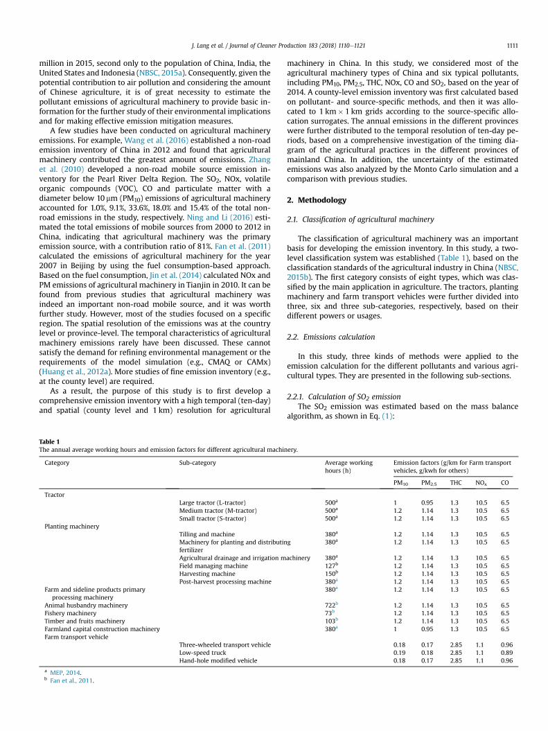
Table 1The annual average working hours and emission factors for different agricultural machin

Category Sub-category

TractorLarge tractor (L-tractor)Medium tractor (M-tractor)Small tractor (S-tractor)

Planting machineryTilling and machineMachinery for planting and distributinfertilizerAgricultural drainage and irrigation mField managing machineHarvesting machinePost-harvest processing machine

Farm and sideline products primaryprocessing machinery

Animal husbandry machineryFishery machineryTimber and fruits machineryFarmland capital construction machineryFarm transport vehicle

Three-wheeled transport vehicleLow-speed truckHand-hole modified vehicle

a MEP, 2014.b Fan et al., 2011.

machinery in China. In this study, we considered most of theagricultural machinery types of China and six typical pollutants,including PM10, PM2.5, THC, NOx, CO and SO2, based on the year of2014. A county-level emission inventory was first calculated basedon pollutant- and source-specific methods, and then it was allo-cated to 1 km� 1 km grids according to the source-specific allo-cation surrogates. The annual emissions in the different provinceswere further distributed to the temporal resolution of ten-day pe-riods, based on a comprehensive investigation of the timing dia-gram of the agricultural practices in the different provinces ofmainland China. In addition, the uncertainty of the estimatedemissions was also analyzed by the Monto Carlo simulation and acomparison with previous studies.

2. Methodology

2.1. Classification of agricultural machinery

The classification of agricultural machinery was an importantbasis for developing the emission inventory. In this study, a two-level classification system was established (Table 1), based on theclassification standards of the agricultural industry in China (NBSC,2015b). The first category consists of eight types, which was clas-sified by the main application in agriculture. The tractors, plantingmachinery and farm transport vehicles were further divided intothree, six and three sub-categories, respectively, based on theirdifferent powers or usages.

2.2. Emissions calculation

In this study, three kinds of methods were applied to theemission calculation for the different pollutants and various agri-cultural types. They are presented in the following sub-sections.

2.2.1. Calculation of SO2 emissionThe SO2 emission was estimated based on the mass balance

algorithm, as shown in Eq. (1):

ery.

Average workinghours (h)

Emission factors (g/km for Farm transportvehicles, g/kwh for others)

PM10 PM2.5 THC NOx CO

500a 1 0.95 1.3 10.5 6.5500a 1.2 1.14 1.3 10.5 6.5500a 1.2 1.14 1.3 10.5 6.5

380a 1.2 1.14 1.3 10.5 6.5g 380a 1.2 1.14 1.3 10.5 6.5

achinery 380a 1.2 1.14 1.3 10.5 6.5127b 1.2 1.14 1.3 10.5 6.5150b 1.2 1.14 1.3 10.5 6.5380a 1.2 1.14 1.3 10.5 6.5380a 1.2 1.14 1.3 10.5 6.5

722b 1.2 1.14 1.3 10.5 6.573b 1.2 1.14 1.3 10.5 6.5103b 1.2 1.14 1.3 10.5 6.5380a 1 0.95 1.3 10.5 6.5

0.18 0.17 2.85 1.1 0.960.19 0.18 2.85 1.1 0.890.18 0.17 2.85 1.1 0.96

J. Lang et al. / Journal of Cleaner Production 183 (2018) 1110e11211112

Ei;j ¼ FCi;j � Si �MSO2

MS� 10�9 (1)

where Ei,j is the SO2 emission (Mg) of the agricultural machinery j inregion i; FC is the annual fuel consumption (kg), which is describedin section 2.3; Si is the sulfur content of the fuel (diesel) - in the yearof 2014, it was 10mg/kg in Beijing, 50mg/kg in Shanghai andGuangzhou, and 350mg/kg in other provinces of mainland China,respectively (Lang et al., 2016); MSO2 (64) and MS (32) are the for-mula weight of SO2 and S, respectively.

2.2.2. Calculation of the agricultural transporter emissionThe emission calculation method for the agricultural transport

vehicles is similar to that for the on-road vehicles, as shown in Eq.(2):

Ei;k ¼Xj

�Pi;j � KTj � EFj;k

�� 10�6 (2)

where Ei,k represents the emission (Mg) of the pollutant k in regioni; Pi,j is the population of the agricultural transport vehicle j in re-gion i; KT is the average annual kilometers travelled (km) of theagricultural transport vehicle - it is 23,000 km, 30,900 km and23,000 km for a three-wheeled transport vehicle, low-speed truckand hand-hole modified vehicle, respectively (MEP, 2014); EF is theemission factor (g/km). The pollutants (k) include PM10, PM2.5, THC,NOx and CO; the population (P) and the emission factor (EF) aredescribed in section 2.3.

2.2.3. Calculation of agricultural machinery emissionThe engine power-based approach was used to calculate the

emission of agricultural machinery, except for agricultural trans-port vehicles, as shown in Eq. (3):

Ei;k ¼Xj

�Pj � Gi;j � LFj � Tj � EFj;k

�� 10�6 (3)

where Ei, k is the total emission (Mg) of the pollutant k in region i; Pjis the population of the agricultural machinery j; G is the averageinstalled engine power (kw); LF is the load factor (0.65) (MEP,2014); T is the average agricultural machinery activity time (h) in

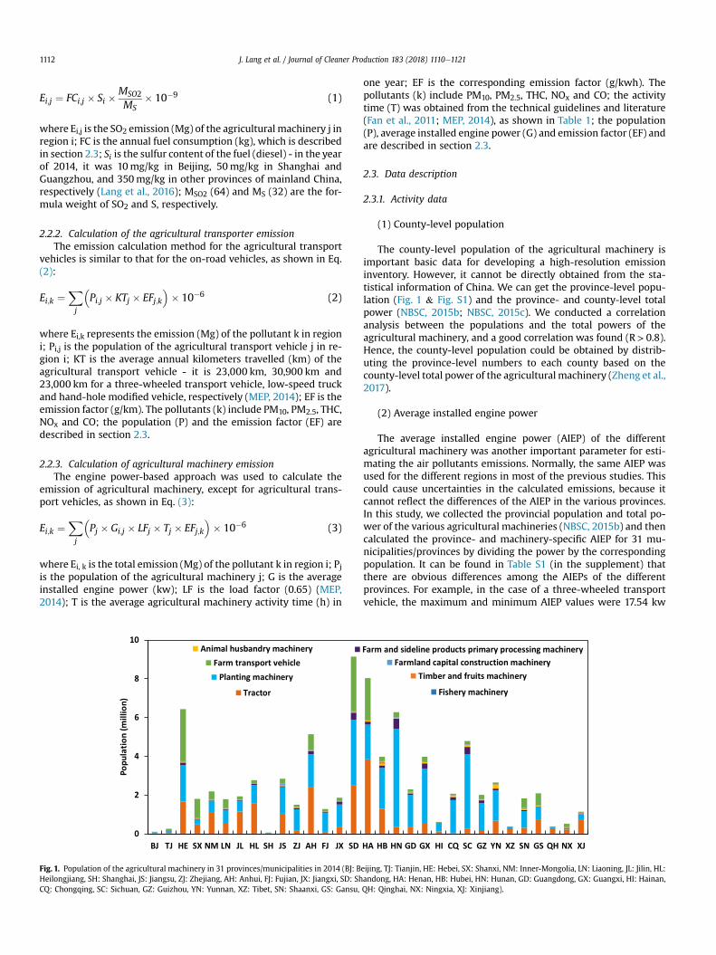
Fig. 1. Population of the agricultural machinery in 31 provinces/municipalities in 2014 (BJ: BHeilongjiang, SH: Shanghai, JS: Jiangsu, ZJ: Zhejiang, AH: Anhui, FJ: Fujian, JX: Jiangxi, SD: ShCQ: Chongqing, SC: Sichuan, GZ: Guizhou, YN: Yunnan, XZ: Tibet, SN: Shaanxi, GS: Gansu,

one year; EF is the corresponding emission factor (g/kwh). Thepollutants (k) include PM10, PM2.5, THC, NOx and CO; the activitytime (T) was obtained from the technical guidelines and literature(Fan et al., 2011; MEP, 2014), as shown in Table 1; the population(P), average installed engine power (G) and emission factor (EF) andare described in section 2.3.

2.3. Data description

2.3.1. Activity data

(1) County-level population

The county-level population of the agricultural machinery isimportant basic data for developing a high-resolution emissioninventory. However, it cannot be directly obtained from the sta-tistical information of China. We can get the province-level popu-lation (Fig. 1 & Fig. S1) and the province- and county-level totalpower (NBSC, 2015b; NBSC, 2015c). We conducted a correlationanalysis between the populations and the total powers of theagricultural machinery, and a good correlation was found (R> 0.8).Hence, the county-level population could be obtained by distrib-uting the province-level numbers to each county based on thecounty-level total power of the agricultural machinery (Zheng et al.,2017).

(2) Average installed engine power

The average installed engine power (AIEP) of the differentagricultural machinery was another important parameter for esti-mating the air pollutants emissions. Normally, the same AIEP wasused for the different regions in most of the previous studies. Thiscould cause uncertainties in the calculated emissions, because itcannot reflect the differences of the AIEP in the various provinces.In this study, we collected the provincial population and total po-wer of the various agricultural machineries (NBSC, 2015b) and thencalculated the province- and machinery-specific AIEP for 31 mu-nicipalities/provinces by dividing the power by the correspondingpopulation. It can be found in Table S1 (in the supplement) thatthere are obvious differences among the AIEPs of the differentprovinces. For example, in the case of a three-wheeled transportvehicle, the maximum and minimum AIEP values were 17.54 kw

eijing, TJ: Tianjin, HE: Hebei, SX: Shanxi, NM: Inner-Mongolia, LN: Liaoning, JL: Jilin, HL:andong, HA: Henan, HB: Hubei, HN: Hunan, GD: Guangdong, GX: Guangxi, HI: Hainan,QH: Qinghai, NX: Ningxia, XJ: Xinjiang).

J. Lang et al. / Journal of Cleaner Production 183 (2018) 1110e1121 1113

and 7.89kw in Chongqing and Zhejiang, respectively. If the meanAIEP of different provinces (12.70 kw) is used for estimating thepollutant emissions, the error would be �27.6% and 61.1% forChongqing and Zhejiang, respectively. The standard deviation (SD,1.97 kw) of the AIEP in different provinces was further calculated,accounting for 15.5% (SD/MEAN) of the mean value. The SD/MEANvalues for the other agricultural machinery were also estimated(Table S1), and the change rangewas 7.7%-84.3%, with a mean valueof 33.6%. These indicate that the calculation of the province-specificAIEP was necessary, and it could decrease the uncertainty of theemissions to a great extent.

(3) Diesel consumption

The diesel consumption was used for the calculation of the SO2emissions. The provincial level sum of the diesel consumption wasobtained from the China Agricultural Machinery Industry Yearbook(NBSC, 2015b), which is shown in Table S2 of the supplement. Thecounty-level fuel consumption values were calculated by using thesame method used for the county-level population based on theprovincial diesel consumption and the county-level total power ofthe agricultural machinery (Fan et al., 2011; Pan et al., 2015; Wei,2013).

2.3.2. Emissions factorThe emission factor is also an important parameter for estab-

lishing the atmospheric pollutant emission inventory. In this study,the emission factors are referred to as the Non-road Mobile SourceEmissions Inventory Compiled Technical Guidelines (MEP, 2014).They are listed in Table 1.

The sources of the data discussed in this section, including theactivity data and the emission factors, are summarized in Table S3.

2.4. Spatial distribution

To improve the resolution of the emission inventory and toprovide the grid emissions for a model simulation, the emissions ofthe different counties were allocated into 1 km� 1 km grid cells.GIS (Geographic Information System) software was the main toolfor conducting the spatial distribution. Source-specific allocationsurrogates were used according to the homologous agriculturalmachinery characteristics: (1) for tractors, planting machinery,farmland capital construction machinery and farm transport vehi-cles, we selected croplands land cover to allocate the countyemissions to grids; (2) for timber and fruit machinery, forest landcover was the distribution basis; (3) for farm and sideline products,primary processing machinery and animal husbandry machinery,rural population density was the proxy; and (4) for fishery ma-chinery, fisherman density was the allocation surrogate. Croplandsland cover and forest land cover were screened from the land usedata (MODIS land cover) provided by Ran et al. (2010). The ruralpopulation density was obtained from satellite data by intersecting

Table 2The sowing and harvest times of the main crops in China.

Crop Sowing time

Wheat Spring wheat Late March to eWinter wheat Mid- to late Sep

Maize Spring maize Late April to earSummer maize Late May to earAutumn maize Early to mid-Jul

Rice Early rice Late March to eMedium rice Early April to eaLate rice Late June to ear

croplands land cover and population. The fisherman density wasobtained based on land use cover and population satellite data.

We allocated emissions to a grid by using the followingequation:

Ei ¼Xi

Xm� Em (4)

where Ei is the emission in the ith grid; Xi is the croplands density,forest density, rural population density or fisherman density in theith grid; Xm is the total croplands density, forest density, ruralpopulation density or fisherman density in the county m; and Em isthe total emissions from the tractors, planting machinery, farmlandcapital constructionmachinery, farm transport vehicles, timber andfruit machinery, farm, sideline, products primary processing ma-chinery, animal husbandry machinery or fishery machinery in thecounty m.

2.5. Temporal allocation

To obtain the temporal variation of the agricultural machineryemissions, the ten-day uneven coefficients had to be determined.This study conducted a comprehensive investigation on the timingdiagram of the agricultural practices in the different provinces ofmainland China, referring to the agricultural practice information(MOA, 2014) and literature (Huang et al., 2012b; Li et al., 2016; Qiuet al., 2016; Zhou et al., 2015, 2017). The plant regions, sow time andharvest time of the main crops in the different provinces of China,including wheat, maize and rice, were surveyed and summarized.Based on the differences of the farming time, wheat was dividedinto springwheat andwinter wheat; maizewas divided into spring,summer and autumn maize; and rice was divided into early, me-dium and late rice. The sowing and harvest time of the main cropsare shown in Table 2.

Based on the service conditions of the different agriculturalmachinery throughout the year, we classified the agricultural ma-chinery into four categories. The ten-day uneven coefficients of theemissions were calculated as described in the following sections.

2.5.1. Types needing service throughout the yearFarm transport vehicles, farmland capital construction ma-

chinery, farm and sideline products, primary processing machineryand animal husbandry machinery were the types needing servicethroughout the year. The calculation method of the emission ten-day uneven coefficient for these types are shown in Eq. (5):

Ck ¼136

(5)

where C is the ten-day uneven coefficient; k indicates the k-thworking ten-day periods; and 36 represents the total number of theten-day periods in a year.

Harvest time

arly April Mid- to late Julytember to early October Late May to mid- to late Junely May Late Augustly June Mid- to late Octobery Late September to early Octoberarly April Mid- to late Julyrly May Mid- to late Septemberly July Early to mid-November

J. Lang et al. / Journal of Cleaner Production 183 (2018) 1110e11211114

2.5.2. Types needing service during specific periodsThese types had specific working periods (e.g., fishing season

and cutting period) in a year, including the fishery machinery,timber and fruits machinery, agricultural drainage and irrigationmachinery, field managing machine and post-harvest processingmachine. The calculation method of the ten-day emission unevencoefficient during the working periods for this type is shown in Eq.(6):

Ci;k ¼1

Ni;ten�days(6)

where C is the ten-day uneven coefficient; k indicates the k-thworking ten-day periods; and Ni;ten�days is the number of theworking ten-day periods for machinery i.

Table 3The emissions of the agricultural machinery in the different provinces/municipal-ities of China in 2014 (Gg).

2.5.3. Types needing service influenced by the farming practice anddifferent crops

The service time of these types was influenced by the farmingpractices and different main crops (e.g., wheat, maize and rice).These types included tilling land machine, equipment for plantingand distributing fertilizer and harvesting machine. Eq. (7) showsthe calculation method of the emission ten-day uneven coefficient.

Ci;j;k ¼Ai;jPjAi;j

� 1Ni;j;ten�days

(7)

where C is the ten-day uneven coefficient; i is the machinery typementioned above; j indicates the main crop type (i.e., wheat, maizeand rice); k indicates the k-th working ten day; A is the area of themechanization (i.e. machine-plowed, machine-sown or machine-harvested) (NBSC, 2015b); and Ni;j;ten�days is the number of theworking ten-day periods for the machinery i used for the crop typej.

Area PM10 PM2.5 THC NOx CO SO2

Beijing 0.32 0.31 2.27 2.60 1.80 0.0016Tianjin 1.07 1.02 8.81 8.40 5.96 0.12Hebei 26.13 24.76 200.04 202.57 142.69 2.16Shanxi 8.16 7.73 72.11 61.98 44.65 0.62Inner-Mongolia 10.86 10.31 37.89 92.67 59.95 0.91Liaoning 6.88 6.52 37.58 56.48 37.98 0.68Jilin 9.02 8.57 21.19 79.30 50.11 1.08Heilongjiang 15.36 14.59 27.91 138.25 86.60 1.66Shanghai 0.15 0.14 0.18 1.45 0.90 0.0035Jiangsu 10.54 10.00 27.78 95.36 60.51 1.07Zhejiang 2.66 2.52 10.27 23.10 14.98 0.86Anhui 16.40 15.56 70.33 138.21 90.84 1.10Fujian 1.98 1.88 9.37 16.44 10.86 0.29Jiangxi 4.74 4.50 16.52 39.90 25.72 0.73Shandong 33.36 31.63 214.61 267.40 183.48 2.80Henan 33.33 31.62 173.68 273.56 183.28 2.58Hubei 9.47 9.00 26.58 82.50 52.53 1.01Hunan 11.73 11.14 32.26 100.28 63.80 1.31Guangdong 4.36 4.14 14.36 37.02 23.76 0.12Guangxi 7.62 7.24 25.20 64.64 41.70 0.94Hainan 1.27 1.21 3.41 10.98 6.98 0.18Chongqing 2.79 2.65 7.37 23.69 15.06 0.36Sichuan 7.06 6.71 19.26 60.44 38.43 0.99Guizhou 4.37 4.14 20.19 35.38 23.22 0.31Yunnan 7.29 6.92 14.15 63.43 39.77 0.59Tibet 1.71 1.63 4.46 14.53 9.21 0.19Shaanxi 5.76 5.46 38.33 45.98 31.66 0.64Gansu 7.50 7.11 47.54 59.25 40.67 0.90Qinghai 1.37 1.30 2.77 11.80 7.43 0.08Ningxia 2.19 2.08 12.99 17.64 11.98 0.16Xinjiang 7.25 6.89 11.97 66.79 41.66 0.75

Total 262.69 249.25 1211.39 2192.05 1448.16 25.14

2.5.4. Type needing complex serviceThe last type was tractors, which are widely used for farming-

related work and transportation. The emission ten-day unevencoefficients were calculated as shown in Eq. (8) for transportationand Eq. (9) for farming-related work.

CT ;k ¼8� NT ;ten�days

8� NT ;ten�days þ 24� NF;ten�days� 1NT;ten�days

(8)

CF;i; j;k ¼Ai;jPiP

jAi;j� 1NF;i;j;ten�days

(9)

where C is the ten-day uneven coefficient; i represents the differentmain crops (i.e. wheat, maize and rice); j is the type of agriculturalactivity (i.e. plowing, sowing and harvesting); k indicates the k-thworking ten-day; A is the area of mechanization; NT ;ten�daysis thenumber of working ten-days for transportation; NF;ten�days is thenumber of the ten-day for farming-relatedwork; andNF;i;j;ten�days isthe number of the ten-day worked for the activity j of crop i. Inaddition, 8 and 24 represent the working hours in a transportationday and in a farming work day, respectively. During the busyfarming periods, the time for the farming work was tight and theduty was heavy, as a result, we assumed that the tractor worked24 h every day. During the normal working days for transportation,we supposed that the tractor worked 8 h per day.

3. Results and discussion

3.1. Total emissions in China

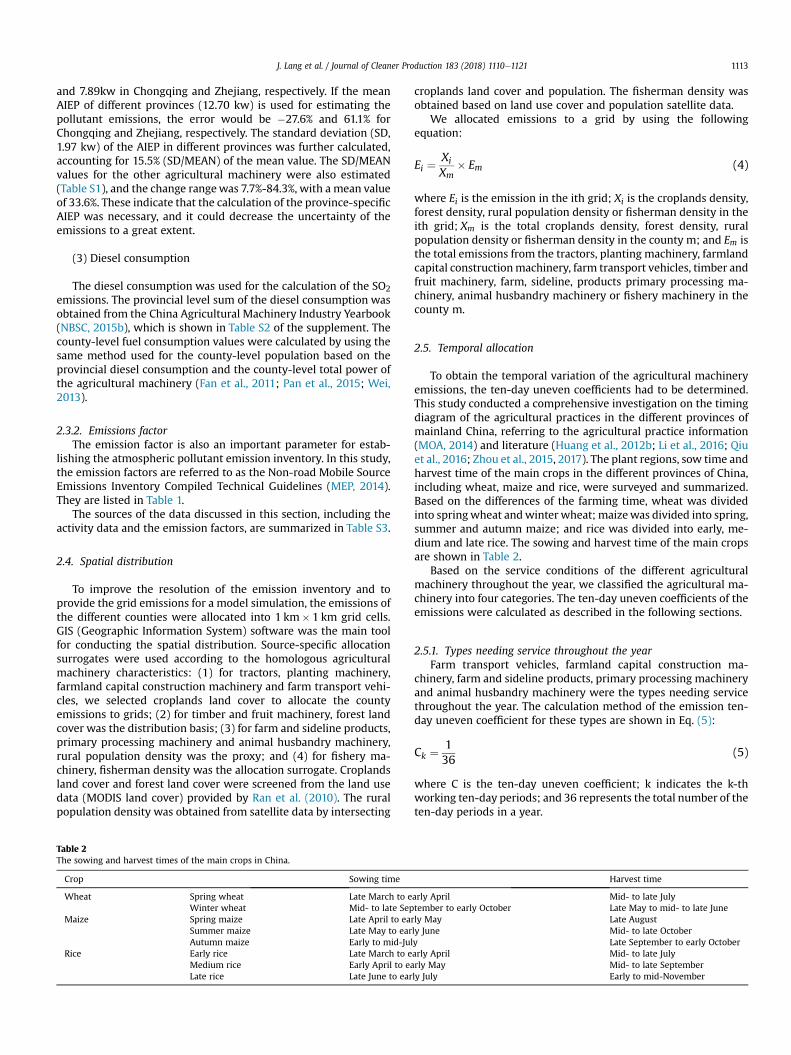
Based on the methods described in section 2, the air pollutantemissions of agricultural machinery in mainland China werecalculated. Table 3 lists the emissions of the different provinces. In2014, the total emissions of PM10, PM2.5, THC, NOx, CO and SO2 forthe Chinese mainland were 262.69 Gg, 249.25 Gg, 1211.39 Gg,2192.05 Gg, 1448.16 Gg and 25.14 Gg, respectively. They wereapproximately 71.9%, 83.0%, 36.4%, 34.5%, 5.2% and 13.0% of theemissions from the on-road vehicles (Lang et al., 2014, 2016),indicating that agricultural machinery was also a non-ignorablesource for air pollutants, especially for the PM, THC and NOxemissions. These pollutants were important precursors of the at-mospheric PM2.5 pollution (Lang et al., 2017), which is the majorenvironmental pollution problem in most areas of China. Conse-quently, the emissions of agricultural machinery, their environ-mental implications and their control should be paid attention to,in addition to the motor vehicles. Among the 31 municipalities/provinces, Shandong, Henan, Hebei, Anhui, Hunan Heilongjiang,Inner-Mongolia and Jiangsu are the top eight provinces with thegreatest amount of emissions in China. They accounted for 60.0%,60.0%, 64.8%, 59.7%, 60.2% and 54.0% of the total PM10, PM2.5, THC,NOx, CO, and SO2 emissions, respectively. Conversely, Beijing,Shanghai, Tianjin, Fujian, Hainan, Tibet, Qinghai and Ningxia arethe eight provinces/municipalities with the least emissions, ac-counting for 3.8%, 3.8%, 3.7%, 3.8%, 3.8% and 4.1% of the total PM10,PM2.5, THC, NOx, CO, and SO2 emissions, respectively. These find-ings were consistent with the development of the agricultural levelin these different regions. By using PM2.5 as an example, Fig. 2

Fig. 2. Correlation between PM2.5 emissions and agricultural related data in different provinces.

J. Lang et al. / Journal of Cleaner Production 183 (2018) 1110e1121 1115

shows that the emissions had an obvious positive correlation withthe cultivated area (R¼ 0.93), total population (R¼ 0.90), agricul-tural production (R¼ 0.82), grain output (R¼ 0.87), rural popula-tion (R¼ 0.82) and primary industry (R¼ 0.82).

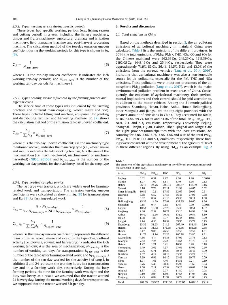
Fig. 3 illustrates the contributions of the main agricultural ma-chineries to the different pollutants. It was found that (1) tractorscontributed the most to the pollutants, except for THC, and thecontribution ratios were 48.9%, 48.9%, 53.6%, 50.2% and 39.9% forPM10, PM2.5, NOx, CO and SO2, respectively; (2) another importantcontributor to emissions, especially THC emissions, is the farmtransport vehicle, and the contribution percentages were 81.8% forTHC and 17.4%-24.6% for the other pollutants; and (3) plantingmachinery also had considerable contributions, with fractions of4.8%-27.9% for the different pollutants. A larger population of thethree agricultural machineries (with a sum percentage of 98.6%)

Fig. 3. Contributions of different agricultural machin

(Fig. 1) and a higher THC emission factor (Table 1) of the farmtransport vehicles were the main reasons for the higher contribu-tion ratios. These indicate that the emission control emphasis of theagricultural machinery should be focused on the tractors, farmtransport vehicles and planting machinery.

3.2. Spatial distribution of emissions

Based on the methods described in sections 2.2 and 2.4, weestimated the county-level (2836 counties in the 31 municipalities/provinces) agricultural machinery emissions, and distributed theminto 1 km � 1 km grids. The emissions maps for all of the species(PM10, PM2.5, THC, NOx, CO, SO2) presented similar spatial distri-butions. Thus, we use PM2.5 as an example to discuss the spatialdistribution characteristics in the following section.

ery types to various pollutants in China in 2014.

J. Lang et al. / Journal of Cleaner Production 183 (2018) 1110e11211116

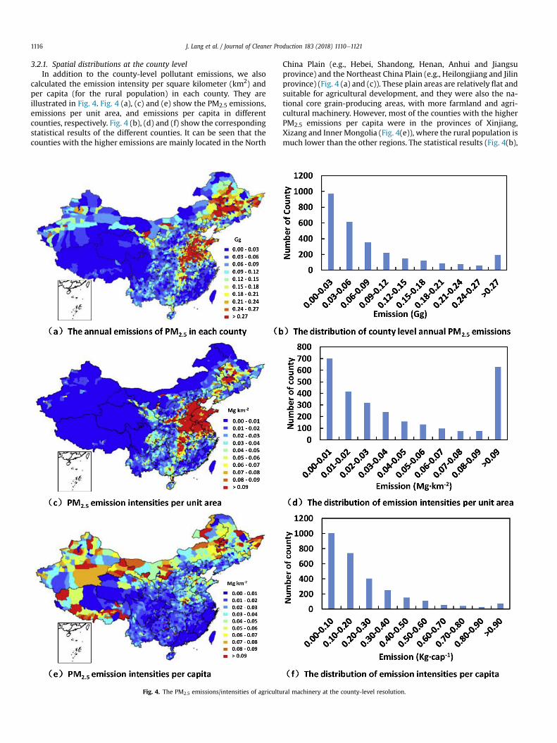
3.2.1. Spatial distributions at the county levelIn addition to the county-level pollutant emissions, we also

calculated the emission intensity per square kilometer (km2) andper capita (for the rural population) in each county. They areillustrated in Fig. 4. Fig. 4 (a), (c) and (e) show the PM2.5 emissions,emissions per unit area, and emissions per capita in differentcounties, respectively. Fig. 4 (b), (d) and (f) show the correspondingstatistical results of the different counties. It can be seen that thecounties with the higher emissions are mainly located in the North

Fig. 4. The PM2.5 emissions/intensities of agricultu

China Plain (e.g., Hebei, Shandong, Henan, Anhui and Jiangsuprovince) and the Northeast China Plain (e.g., Heilongjiang and Jilinprovince) (Fig. 4 (a) and (c)). These plain areas are relatively flat andsuitable for agricultural development, and they were also the na-tional core grain-producing areas, with more farmland and agri-cultural machinery. However, most of the counties with the higherPM2.5 emissions per capita were in the provinces of Xinjiang,Xizang and Inner Mongolia (Fig. 4(e)), where the rural population ismuch lower than the other regions. The statistical results (Fig. 4(b),

ral machinery at the county-level resolution.

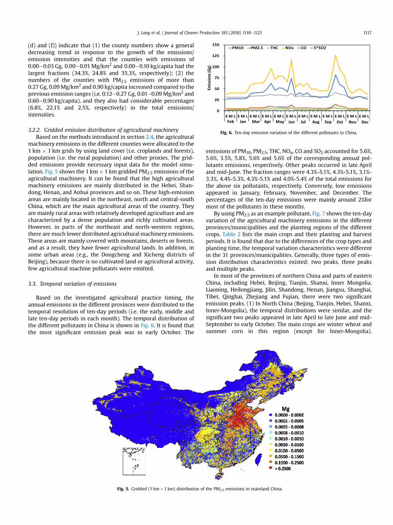
Fig. 6. Ten-day emission variation of the different pollutants in China.

J. Lang et al. / Journal of Cleaner Production 183 (2018) 1110e1121 1117

(d) and (f)) indicate that (1) the county numbers show a generaldecreasing trend in response to the growth of the emissions/emission intensities and that the counties with emissions of0.00e0.03 Gg, 0.00e0.01Mg/km2 and 0.00e0.10 kg/capita had thelargest fractions (34.3%, 24.8% and 35.3%, respectively); (2) thenumbers of the counties with PM2.5 emissions of more than0.27 Gg, 0.09Mg/km2 and 0.90 kg/capita increased compared to theprevious emission ranges (i.e. 0.12e0.27 Gg, 0.01e0.09Mg/km2 and0.60e0.90 kg/capita), and they also had considerable percentages(6.8%, 22.1% and 2.5%, respectively) in the total emissions/intensities.

3.2.2. Gridded emission distribution of agricultural machineryBased on the methods introduced in section 2.4, the agricultural

machinery emissions in the different counties were allocated to the1 km � 1 km grids by using land cover (i.e. croplands and forests),population (i.e. the rural population) and other proxies. The grid-ded emissions provide necessary input data for the model simu-lation. Fig. 5 shows the 1 km � 1 km gridded PM2.5 emissions of theagricultural machinery. It can be found that the high agriculturalmachinery emissions are mainly distributed in the Hebei, Shan-dong, Henan, and Anhui provinces and so on. These high-emissionareas are mainly located in the northeast, north and central-southChina, which are the main agricultural areas of the country. Theyare mainly rural areas with relatively developed agriculture and arecharacterized by a dense population and richly cultivated areas.However, in parts of the northeast and north-western regions,there aremuch lower distributed agricultural machinery emissions.These areas are mainly covered with mountains, deserts or forests,and as a result, they have fewer agricultural lands. In addition, insome urban areas (e.g., the Dongcheng and Xicheng districts ofBeijing), because there is no cultivated land or agricultural activity,few agricultural machine pollutants were emitted.

3.3. Temporal variation of emissions

Based on the investigated agricultural practice timing, theannual emissions in the different provinces were distributed to thetemporal resolution of ten-day periods (i.e. the early, middle andlate ten-day periods in each month). The temporal distribution ofthe different pollutants in China is shown in Fig. 6. It is found thatthe most significant emission peak was in early October. The

Fig. 5. Gridded (1 km� 1 km) distribution of

emissions of PM10, PM2.5, THC, NOx, CO and SO2 accounted for 5.6%,5.6%, 3.5%, 5.8%, 5.6% and 5.6% of the corresponding annual pol-lutants emissions, respectively. Other peaks occurred in late Apriland mid-June. The fraction ranges were 4.3%-5.1%, 4.3%-5.1%, 3.1%-3.3%, 4.4%-5.3%, 4.3%-5.1% and 4.0%-5.4% of the total emissions forthe above six pollutants, respectively. Conversely, low emissionsappeared in January, February, November, and December. Thepercentages of the ten-day emissions were mainly around 2%formost of the pollutants in these months.

By using PM2.5 as an example pollutant, Fig. 7 shows the ten-dayvariation of the agricultural machinery emissions in the differentprovinces/municipalities and the planting regions of the differentcrops. Table 2 lists the main crops and their planting and harvestperiods. It is found that due to the differences of the crop types andplanting time, the temporal variation characteristics were differentin the 31 provinces/municipalities. Generally, three types of emis-sion distribution characteristics existed: two peaks, three peaksand multiple peaks.

In most of the provinces of northern China and parts of easternChina, including Hebei, Beijing, Tianjin, Shanxi, Inner Mongolia,Liaoning, Heilongjiang, Jilin, Shandong, Henan, Jiangsu, Shanghai,Tibet, Qinghai, Zhejiang and Fujian, there were two significantemission peaks. (1) In North China (Beijing, Tianjin, Hebei, Shanxi,Inner-Mongolia), the temporal distributions were similar, and thesignificant two peaks appeared in late April to late June and mid-September to early October. The main crops are winter wheat andsummer corn in this region (except for Inner-Mongolia).

the PM2.5 emissions in mainland China.

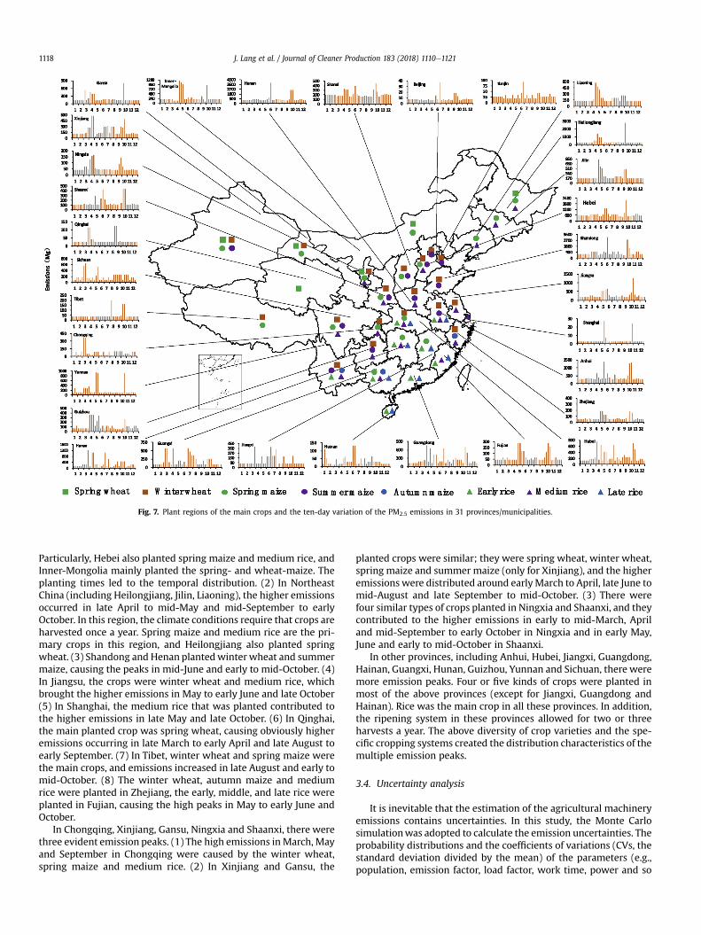
Fig. 7. Plant regions of the main crops and the ten-day variation of the PM2.5 emissions in 31 provinces/municipalities.

J. Lang et al. / Journal of Cleaner Production 183 (2018) 1110e11211118

Particularly, Hebei also planted spring maize and medium rice, andInner-Mongolia mainly planted the spring- and wheat-maize. Theplanting times led to the temporal distribution. (2) In NortheastChina (including Heilongjiang, Jilin, Liaoning), the higher emissionsoccurred in late April to mid-May and mid-September to earlyOctober. In this region, the climate conditions require that crops areharvested once a year. Spring maize and medium rice are the pri-mary crops in this region, and Heilongjiang also planted springwheat. (3) Shandong and Henan plantedwinter wheat and summermaize, causing the peaks in mid-June and early to mid-October. (4)In Jiangsu, the crops were winter wheat and medium rice, whichbrought the higher emissions in May to early June and late October(5) In Shanghai, the medium rice that was planted contributed tothe higher emissions in late May and late October. (6) In Qinghai,the main planted crop was spring wheat, causing obviously higheremissions occurring in late March to early April and late August toearly September. (7) In Tibet, winter wheat and spring maize werethe main crops, and emissions increased in late August and early tomid-October. (8) The winter wheat, autumn maize and mediumrice were planted in Zhejiang, the early, middle, and late rice wereplanted in Fujian, causing the high peaks in May to early June andOctober.

In Chongqing, Xinjiang, Gansu, Ningxia and Shaanxi, there werethree evident emission peaks. (1) The high emissions inMarch, Mayand September in Chongqing were caused by the winter wheat,spring maize and medium rice. (2) In Xinjiang and Gansu, the

planted crops were similar; they were spring wheat, winter wheat,spring maize and summer maize (only for Xinjiang), and the higheremissions were distributed around earlyMarch to April, late June tomid-August and late September to mid-October. (3) There werefour similar types of crops planted in Ningxia and Shaanxi, and theycontributed to the higher emissions in early to mid-March, Apriland mid-September to early October in Ningxia and in early May,June and early to mid-October in Shaanxi.

In other provinces, including Anhui, Hubei, Jiangxi, Guangdong,Hainan, Guangxi, Hunan, Guizhou, Yunnan and Sichuan, there weremore emission peaks. Four or five kinds of crops were planted inmost of the above provinces (except for Jiangxi, Guangdong andHainan). Rice was the main crop in all these provinces. In addition,the ripening system in these provinces allowed for two or threeharvests a year. The above diversity of crop varieties and the spe-cific cropping systems created the distribution characteristics of themultiple emission peaks.

3.4. Uncertainty analysis

It is inevitable that the estimation of the agricultural machineryemissions contains uncertainties. In this study, the Monte Carlosimulationwas adopted to calculate the emission uncertainties. Theprobability distributions and the coefficients of variations (CVs, thestandard deviation divided by the mean) of the parameters (e.g.,population, emission factor, load factor, work time, power and so

J. Lang et al. / Journal of Cleaner Production 183 (2018) 1110e1121 1119

on, as shown in Eqs. (1)e(3)), must be confirmed first. Consideringthat (1) the quantitative uncertainty analysis of the agriculturalmachinery emissions seldom has been conducted, and (2) theemission characteristics were similar to the on-road vehicles, weassumed that the probability distributions and CVs of some pa-rameters used for the agricultural machinery are the same as thosefor the on-road vehicles (Zhao et al., 2011). Therefore, a normaldistributionwith a CV of 5%was used for the population (Zhao et al.,2011; Lang et al., 2014, 2016). For the emission factors, the distri-butionwas assumed to be lognormal. The different emission factorshad different CVs. The CVs were 47%, 47%, 57%, 33% and 92% forPM10, PM2.5, THC, NOx and CO, respectively (Wang et al., 2016). Forthe load factor, power and work time, there is a lack of statisticalinformation, and in this study, the distributionswere assumed to benormal with a CV of 30%. The mileage was assumed to be a normaldistribution with a CV of 30%, based on Lang et al.’s (2014) study. Inaddition, the distributions of the fuel consumption and sulfurcontent were used as normal with a CV of 16% (Karvosenoja et al.,2008) and 5%, respectively. After the above setting of parameters,100,000 simulations were performed to calculate the uncertaintiesof the emissions. The uncertainty ranges (95% confidence intervals)of the total PM10, PM2.5, THC, NOx, CO and SO2 emissionswere �43.9% to 60.9%, �43.6%e60.9%, �71.0%e90.9%, �33.0%e43.3%, �73.2%e93.7%, and �10.7% to 10.8%, respectively.

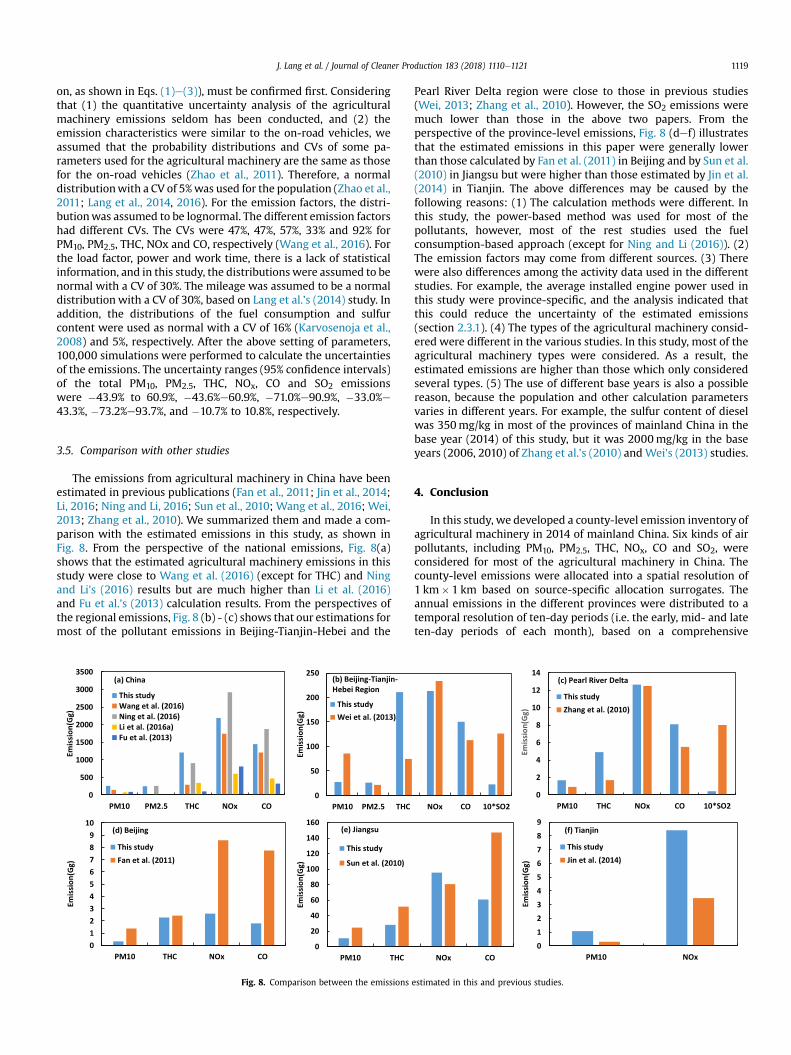
3.5. Comparison with other studies

The emissions from agricultural machinery in China have beenestimated in previous publications (Fan et al., 2011; Jin et al., 2014;Li, 2016; Ning and Li, 2016; Sun et al., 2010; Wang et al., 2016; Wei,2013; Zhang et al., 2010). We summarized them and made a com-parison with the estimated emissions in this study, as shown inFig. 8. From the perspective of the national emissions, Fig. 8(a)shows that the estimated agricultural machinery emissions in thisstudy were close to Wang et al. (2016) (except for THC) and Ningand Li's (2016) results but are much higher than Li et al. (2016)and Fu et al.’s (2013) calculation results. From the perspectives ofthe regional emissions, Fig. 8 (b) - (c) shows that our estimations formost of the pollutant emissions in Beijing-Tianjin-Hebei and the

Fig. 8. Comparison between the emissions

Pearl River Delta region were close to those in previous studies(Wei, 2013; Zhang et al., 2010). However, the SO2 emissions weremuch lower than those in the above two papers. From theperspective of the province-level emissions, Fig. 8 (def) illustratesthat the estimated emissions in this paper were generally lowerthan those calculated by Fan et al. (2011) in Beijing and by Sun et al.(2010) in Jiangsu but were higher than those estimated by Jin et al.(2014) in Tianjin. The above differences may be caused by thefollowing reasons: (1) The calculation methods were different. Inthis study, the power-based method was used for most of thepollutants, however, most of the rest studies used the fuelconsumption-based approach (except for Ning and Li (2016)). (2)The emission factors may come from different sources. (3) Therewere also differences among the activity data used in the differentstudies. For example, the average installed engine power used inthis study were province-specific, and the analysis indicated thatthis could reduce the uncertainty of the estimated emissions(section 2.3.1). (4) The types of the agricultural machinery consid-ered were different in the various studies. In this study, most of theagricultural machinery types were considered. As a result, theestimated emissions are higher than those which only consideredseveral types. (5) The use of different base years is also a possiblereason, because the population and other calculation parametersvaries in different years. For example, the sulfur content of dieselwas 350mg/kg in most of the provinces of mainland China in thebase year (2014) of this study, but it was 2000mg/kg in the baseyears (2006, 2010) of Zhang et al.’s (2010) and Wei's (2013) studies.

4. Conclusion

In this study, we developed a county-level emission inventory ofagricultural machinery in 2014 of mainland China. Six kinds of airpollutants, including PM10, PM2.5, THC, NOx, CO and SO2, wereconsidered for most of the agricultural machinery in China. Thecounty-level emissions were allocated into a spatial resolution of1 km� 1 km based on source-specific allocation surrogates. Theannual emissions in the different provinces were distributed to atemporal resolution of ten-day periods (i.e. the early, mid- and lateten-day periods of each month), based on a comprehensive

estimated in this and previous studies.

J. Lang et al. / Journal of Cleaner Production 183 (2018) 1110e11211120

investigation of the main crop farming timing in China.The results showed that the total annual emissions of PM10,

PM2.5, THC, NOx, CO and SO2 for the Chinese mainland were262.69 Gg, 249.25 Gg, 1211.39 Gg, 2192.05 Gg, 1448.16 Gg and25.14 Gg, respectively. They were approximately 71.9%, 83.0%,36.4%, 34.5%, 5.2% and 13.0% of the emissions from the on-roadvehicles in mainland China. The tractors, farm transport vehiclesand planting machinery are the main contributors of the differentpollutants. The gridded emission results indicate that the higheragricultural machinery emissions are distributed in the northeast,north and central-south regions of China.

The temporal distribution of the total emissions in Chinashowed that the higher emissions occurred in late April, mid-Juneand early October. Three types of emission distribution character-istics existed in the different provinces: two peaks, three peaks andmultiple peaks. Hebei, Beijing, Tianjin, Shanxi, Inner Mongolia,Liaoning, Heilongjiang, Jilin, Shandong, Henan, Jiangsu, Shanghai,Tibet, Qinghai, Zhejiang and Fujian had two significant emissionpeaks. Chongqing, Xinjiang, Gansu, Ningxia and Shaanxi had threeemission peaks. Anhui, Hubei, Jiangxi, Guangdong, Hainan,Guangxi, Hunan, Guizhou, Yunnan and Sichuan had multipleemission peaks.

The uncertainties of the agricultural machinery pollutantemissions were analyzed by the Monte Carlo simulation. The totaluncertainty ranges (95% confidence intervals) were �43.9% to60.9%, �43.6%e60.9%, �71.0%e90.9%, �33.0%e43.3%, �73.2%e93.7%, and �10.7% to 10.8%, for PM10, PM2.5, THC, NOx, CO and SO2,respectively.

Acknowledgement

This research was supported by the Natural Sciences Foundationof China (No. 91644110, 51408014 & 51308257) and the New TalentProgram of Beijing University of Technology (No. 2017-RX(1)-10). Inaddition, we greatly appreciated Beijing Municipal Commission ofEducation and Beijing Municipal Commission of Science andTechnology for supporting this work. The authors are grateful to theanonymous reviewers for their insightful comments.

Appendix A. Supplementary data

Supplementary data related to this article can be found athttps://doi.org/10.1016/j.jclepro.2018.02.120.

References

Anenberg, S.C., Balakrishnan, K., Jetter, J., Masera, O., Mehta, S., Moss, J.,Ramanathan, V., 2013. Cleaner cooking solutions to achieve health, climate, andeconomic cobenefits. Environ. Sci. Technol. 47 (9), 3944e3952.

Fan, S., Nie, L., Kan, R., Li, X., Yang, T., 2011. Fuel consumption based exhaustemissions estimating from agriculture equipment in Beijing. J. Saf. Environ. 11,145e148 (in Chinese).

Fu, M., Ding, Y., Yin, H., Ji, Z., Ge, Y., Liang, B., 2013. Characteristics of agriculturaltractors emissions under real-world operating cycle. Trans. Chin. Soc. Agric.Eng. 29, 42e48 (in Chinese).

Fu, Y., Tai, A.P.K., 2015. Impact of climate and land cover changes on troposphericozone air quality and public health in East Asia between 1980 and 2010. Atmos.Chem. Phys. 15 (17), 10093e10106.

Gu, Y., Yim, S.H.L., 2016. The air quality and health impacts of domestic trans-boundary pollution in various regions of China. Environ. Int. 97, 117e124.

He, J.J., Wu, L., Mao, H.J., Liu, H.L., Jing, B.Y., Yu, Y., Ren, P.P., Feng, C., Liu, X.H., 2016.Development of a vehicle emission inventory with high temporal-spatial res-olution based on NRT traffic data and its impact on air pollution in Beijing - Part2: impact of vehicle emission on urban air quality. Atmos. Chem. Phys. 16 (5),3171e3184.

Huang, Q., Cheng, S.Y., Perozzi, R.E., Perozzi, E.F., 2012a. Use of a MM5-CAMx-PSATmodeling system to study SO2 source apportionment in the Beijing metropol-itan region. Environ. Model. Assess. 17, 527e538.

Huang, X., Song, Y., Li, M.M., Li, J.F., Huo, Q., Cai, X.H., Zhu, T., Hu, M., Zhang, H.S.,2012b. A high-resolution ammonia emission inventory in China. Global

Biogeochem. Cycles 26.Jin, T., Chen, D., Fu, X., Li, Y., Yi, Z., Lu, K., 2014. Estimation agricultural machinery

emissions in Tianjin in 2010 based on fuel consumption. China Environ. Sci. 34,2148e2152 (in Chinese).

Kapadia, Z.Z., Spracklen, D.V., Arnold, S.R., Borman, D.J., Mann, G.W., Pringle, K.J.,Monks, S.A., Reddington, C.L., Benduhn, F., Rap, A., Scott, C.E., Butt, E.W.,Yoshioka, M., 2016. Impacts of aviation fuel sulfur content on climate and hu-man health. Atmos. Chem. Phys. 16 (16), 10521e10541.

Karvosenoja, N., Tainio, M., Kupiainen, K., Tuomisto, J.T., Kukkonen, J., Johansson, M.,2008. Evaluation of the emissions and uncertainties of PM2.5 originated fromvehicular traffic and domestic wood combustion in Finland. Boreal Environ. Res.13 (5), 465e474.

Kodros, J.K., Scott, C.E., Farina, S.C., Lee, Y.H., L'Orange, C., Volckens, J., Pierce, J.R.,2015. Uncertainties in global aerosols and climate effects due to biofuel emis-sions. Atmos. Chem. Phys. 15 (15), 8577e8596.

Lang, J.L., Cheng, S.Y., Zhou, Y., Zhang, Y.L., Wang, G., 2014. Air pollutant emissionsfrom on-road vehicles in China, 1999-2011. Sci. Total Environ. 496, 1e10.

Lang, J.L., Zhou, Y., Cheng, S.Y., Zhang, Y.Y., Dong, M., Li, S.Y., Wang, G., Zhang, Y.L.,2016. Unregulated pollutant emissions from on-road vehicles in China, 1999-2014. Sci. Total Environ. 573, 974e984.

Lang, J.L., Zhou, Y., Chen, D.S., Xing, X.F., Wei, L., Wang, X.T., Zhao, N., Zhang, Y.Y.,Guo, X.R., Han, L.H., Cheng, S.Y., 2017. Investigating the contribution of shippingemissions to atmospheric PM2.5 using a combined source apportionmentapproach. Environ. Pollut. 229, 557e566.

Li, M.Y., 2016. Research of Mobile Source Inventories. Beijing Institute of Technology(in Chinese).

Li, J., Li, Y.Q., Bo, Y., Xie, S.D., 2016. High-resolution historical emission inventories ofcrop residue burning in fields in China for the period 1990-2013. Atmos. En-viron. 138, 152e161.

Liu, H., Fu, M., Jin, X., Shang, Y., Shindell, D., Faluvegi, G., Shindell, C., He, K., 2016.Health and climate impacts of ocean-going vessels in East Asia. Nature Clim.(Change advance online publication).

Liu, M.M., Huang, Y.N., Ma, Z.W., Jin, Z., Liu, X.Y., Wang, H., Liu, Y., Wang, J.N.,Jantunen, M., Bi, J., Kinney, P.L., 2017a. Spatial and temporal trends in themortality burden of air pollution in China: 2004-2012. Environ. Int. 98, 75e81.

Liu, Y.H., Liao, W.Y., Li, L., Huang, Y.T., Xu, W.J., 2017b. Vehicle emission trends inChina's Guangdong Province from 1994 to 2014. Sci. Total Environ. 586,512e521.

Ministry of Environmental Protection of the People’s Republic of China (MEP), 2014.Non-road Mobile Source Emissions Inventory Compiled Technical Guidelines.Available at: http://www.mep.gov.cn/gkml/hbb/bgg/201501/W020150107594587960717.pdf.

Ministry of Agriculture of the People’s Republic of China (MOA), 2014. Database ofFarming Season. Available at: http://www.zzys.mos.gov.cn/.

National Bureau of Statistics of China (NBSC), 2015a. China Statistical Yearbook.China Statistics Press, Beijing.

National Bureau of Statistics of China (NBSC), 2015b. China Agricultural MachineryIndustry Yearbook. China Machine Press, Beijing.

National Bureau of Statistics of China (NBSC), 2015c. China County StatisticalYearbook 2015. China Statistics Press, Beijing.

Ning, Y.L., Li, H., 2016. Estimation for main atmospheric pollutants emissions frommobile sources in China. Chin. J. Environ. Eng. 10, 4435e4444 (in Chinese).

Pan, Y., Li, N., Zheng, J., Yin, S., Li, C., Yang, J., Zhong, L., Chen, D., Deng, S., Wang, S.,2015. Emission inventory and characteristics of anthropogenic air pollutantsources in Guangdong Province. Acta Sci. Circ. 35, 2655e2669 (in Chinese).

Qiu, X.H., Duan, L., Chai, F.H., Wang, S.X., Yu, Q., Wang, S.L., 2016. Deriving high-resolution emission inventory of open biomass burning in China based onsatellite observations. Environ. Sci. Technol. 50 (21), 11779e11786.

Ran, Y.H., Li, X., Lu, L., 2010. Evaluation of four remote sensing based land coverproducts over China. Int. J. Rem. Sens. 31 (2), 391e401.

Sun, J., Lu, G., Liu, S., 2010. Research on status of agricultural pollution in Jiangsuprovince. Chin. Agri. Mech. 1, 25e27, 31(in Chinese).

Wang, F., Li, Z., Zhang, K.S., Di, B.F., Hu, B.M., 2016. An overview of non-roadequipment emissions in China. Atmos. Environ. 132, 283e289.

Wei, X., 2013. Establishment of the non-road mobile source emission inventory inBeijing-Tianjin-Hebei. In: Proceedings of the China Environmental Science As-sociation. China Environmental Science Press, Beijing (in Chinese).

Wu, Y.Y., Gu, B.J., Erisman, J.W., Reis, S., Fang, Y.Y., Lu, X.H., Zhang, X.M., 2016. PM2.5pollution is substantially affected by ammonia emissions in China. Environ.Pollut. 218, 86e94.

Xie, R., Sabel, C.E., Lu, X., Zhu, W.M., Kan, H.D., Nielsen, C.P., Wang, H.K., 2016. Long-term trend and spatial pattern of PM2.5 induced premature mortality in China.Environ. Int. 97, 180e186.

Zhang, L., Zheng, J., Yin, S., Peng, K., Zhong, L., 2010. Development of non-roadmobile source emission inventory for the Pearl River Delta region. Environ.Sci. J. Integr. Environ. Res. 31, 886e891 (in Chinese).

Zhang, Q., Jiang, X.J., Tong, D., Davis, S.J., Zhao, H.Y., Geng, G.N., Feng, T., Zheng, B.,Lu, Z.F., Streets, D.G., Ni, R.J., Brauer, M., van Donkelaar, A., Martin, R.V., Huo, H.,Liu, Z., Pan, D., Kan, H.D., Yan, Y.Y., Lin, J.T., He, K.B., Guan, D.B., 2017. Trans-boundary health impacts of transported global air pollution and internationaltrade. Nature 543 (7647), 705-þ.

Zhao, Y., Nielsen, C.P., Lei, Y., McElroy, M.B., Hao, J., 2011. Quantifying the un-certainties of a bottom-up emission inventory of anthropogenic atmosphericpollutants in China. Atmos. Chem. Phys. 11 (5), 2295e2308.

Zheng, B., Zhang, Q., Tong, D., Chen, C.C., Hong, C.P., Li, M., Geng, G.N., Lei, Y., Huo, H.,

J. Lang et al. / Journal of Cleaner Production 183 (2018) 1110e1121 1121

He, K.B., 2017. Resolution dependence of uncertainties in gridded emissioninventories: a case study in Hebei, China. Atmos. Chem. Phys. 17 (2), 921e933.

Zhou, Y., Cheng, S.Y., Lang, J.L., Chen, D.S., Zhao, B.B., Liu, C., Xu, R., Li, T.T., 2015.A comprehensive ammonia emission inventory with high-resolution and itsevaluation in the Beijing-Tianjin-Hebei (BTH) region, China. Atmos. Environ.

106, 305e317.Zhou, Y., Xing, X., Lang, J., Chen, D., Cheng, S., Wei, L., Wei, X., Liu, C., 2017.

A comprehensive biomass burning emission inventory with high spatial andtemporal resolution in China. Atmos. Chem. Phys. 17 (4), 2839e2864.