Embed Size (px)
Citation preview


Editorial Board
I
JAQM Editorial Board Editors Ion Ivan, University of Economics, Romania Claudiu Herteliu, University of Economics, Romania Gheorghe Nosca, Association for Development through Science and Education, Romania Editorial Team Cristian Amancei, University of Economics, Romania Catalin Boja, University of Economics, Romania Radu Chirvasuta, “Carol Davila” University of Medicine and Pharmacy, Romania Irina Maria Dragan, University of Economics, Romania Eugen Dumitrascu, Craiova University, Romania Matthew Elbeck, Troy University, Dothan, USA Nicu Enescu, Craiova University, Romania Bogdan Vasile Ileanu, University of Economics, Romania Miruna Mazurencu Marinescu, University of Economics, Romania Daniel Traian Pele, University of Economics, Romania Ciprian Costin Popescu, University of Economics, Romania Aura Popa, University of Economics, Romania Marius Popa, University of Economics, Romania Mihai Sacala, University of Economics, Romania Cristian Toma, University of Economics, Romania Erika Tusa, University of Economics, Romania Adrian Visoiu, University of Economics, Romania Manuscript Editor Lucian Naie, SDL Tridion

Advisory Board
II
JAQM Advisory Board Luigi D’Ambra, University of Naples “Federico II”, Italy Ioan Andone, Al. Ioan Cuza University, Romania Kim Viborg Andersen, Copenhagen Business School, Denmark Tudorel Andrei, University of Economics, Romania Gabriel Badescu, Babes-Bolyai University, Romania Catalin Balescu, National University of Arts, Romania Avner Ben-Yair, SCE - Shamoon College of Engineering, Beer-Sheva, Israel Constanta Bodea, University of Economics, Romania Ion Bolun, Academy of Economic Studies of Moldova Recep Boztemur, Middle East Technical University Ankara, Turkey Constantin Bratianu, University of Economics, Romania Irinel Burloiu, Intel Romania Ilie Costas, Academy of Economic Studies of Moldova Valentin Cristea, University Politehnica of Bucharest, Romania Marian-Pompiliu Cristescu, Lucian Blaga University, Romania Victor Croitoru, University Politehnica of Bucharest, Romania Cristian Pop Eleches, Columbia University, USA Michele Gallo, University of Naples L'Orientale, Italy Angel Garrido, National University of Distance Learning (UNED), Spain Bogdan Ghilic Micu, University of Economics, Romania Anatol Godonoaga, Academy of Economic Studies of Moldova Alexandru Isaic-Maniu, University of Economics, Romania Ion Ivan, University of Economics, Romania Radu Macovei, “Carol Davila” University of Medicine and Pharmacy, Romania Dumitru Marin, University of Economics, Romania Dumitru Matis, Babes-Bolyai University, Romania Adrian Mihalache, University Politehnica of Bucharest, Romania Constantin Mitrut, University of Economics, Romania Mihaela Muntean, Western University Timisoara, Romania Ioan Neacsu, University of Bucharest, Romania Peter Nijkamp, Free University De Boelelaan, The Nederlands Stefan Nitchi, Babes-Bolyai University, Romania Gheorghe Nosca, Association for Development through Science and Education, Romania Dumitru Oprea, Al. Ioan Cuza University, Romania Adriean Parlog, National Defense University, Bucharest, Romania Victor Valeriu Patriciu, Military Technical Academy, Romania Perran Penrose, Independent, Connected with Harvard University, USA and London University, UK Dan Petrovici, Kent University, UK Victor Ploae, Ovidius University, Romania Gabriel Popescu, University of Economics, Romania Mihai Roman, University of Economics, Romania Ion Gh. Rosca, University of Economics, Romania Gheorghe Sabau, University of Economics, Romania Radu Serban, University of Economics, Romania Satish Chand Sharma, Janta Vedic College, Baraut, India Ion Smeureanu, University of Economics, Romania Ilie Tamas, University of Economics, Romania Nicolae Tapus, University Politehnica of Bucharest, Romania Timothy Kheng Guan Teo, University of Auckland, New Zeeland Daniel Teodorescu, Emory University, USA Dumitru Todoroi, Academy of Economic Studies of Moldova Nicolae Tomai, Babes-Bolyai University, Romania Victor Voicu, “Carol Davila” University of Medicine and Pharmacy, Romania Vergil Voineagu, University of Economics, Romania

Contents
III
Page
Arfan Raheen AFZAL, Sabrina ALAM Analysis and Comparison of Under Five Child Mortality between Rural and Urban Area in Bangladesh
1
Catalin Alexandru TANASIE Analyzing Internal and External Distributed Application Interdependencies using MERICS
11
Muhammad Naveed KHALID, Cees A. W. GLAS A Step-Wise Method for Evaluation of Differential Item Functioning 25 Gheorghe SAVOIU, Gheorghe CRUCERU
Some Aspects of a Quantitative Market Research: “The Opinions and Attitudes of Renault & Automobile Dacia Car’s Buyer”
48

Quantitative Methods Inquires
1
ANALYSIS AND COMPARISON OF UNDER FIVE CHILD MORTALITY BETWEEN RURAL AND URBAN AREA
IN BANGLADESH
Arfan Raheen AFZAL1 International Centre for Diarrhoeal Disease Research, Bangladesh (ICDDR,B) E-mail: [email protected]
Sabrina ALAM2 International Centre for Diarrhoeal Disease Research, Bangladesh (ICDDR,B)
Abstract: Knowledge of factors that affect the under-five year child mortality is important because it pertains to policy and programs. Causes and differences of under-five mortality between rural and urban area help decision makers to assess programmatic needs and prioritize interventions. This paper investigates the causes and differences of under-five mortality between rural and urban area in Bangladesh using Kaplan-Meier, Cox Proportional Hazard (Cox-PH) and Accelerated Failure Time (AFT) Regression model. Bangladesh Demographic and Health Survey (BDHS)-2007 data are used for the study. The results show that for both the areas, survival probability for children whose mothers have higher education is very high and in urban area the failure rate is very high for children of poor economic status. The Cox-PH analysis reveals that risk of death was lower for children whose mothers were matured and higher educated than younger and no educated mother in rural area. In urban area, children from rich family and the 2nd or 3rd child have lower risk of death compared to poor and 1st child. The AFT analysis shows that for both the areas Weibull distribution better fits the data. Key words: child mortality; urban; rural; Bangladesh; ATF; Cox-PH; KM; BDHS
1 INTRODUCTION AND LITERATURE REVIEW
We are interested in analyzing and comparing child mortality between rural and urban area because identifying these may help the government to correct and formulate its policy to reduce child mortality in Bangladesh. Therefore, the analysis done on child mortality has received considerable attention. This paper provides empirical evidence that,

Quantitative Methods Inquires
2
some covariates influence child mortality where the covariates are: sex and birth order of the child, mother’s age, education and economic status of the child using Kaplan-Meier, Cox Proportional Hazard (Cox-PH) Regression model and Accelerated failure time (AFT) regression model.
Mozumder et al. (1998) obtained data on a cohort of 21,268 children born during 1983-1991 in three rural Project sites obtained from the longitudinal Sample Registration System (SRS) of the MCH-FP Extension Project (Rural) of the International Centre for Diarrhoeal Disease Research, Bangladesh. The data suggest that there is a significant relationship between childhood immunization and reduced child mortality. Access to tubewell water was also associated with a reduced risk of mortality for young children. Baqui and others have reported on causes of death under age five based on verbal autopsy interviews in the 1993-1994 and 1996-1997 BDHS sample (Baqui et al., 1998; Baqui et al., 2001). The study in the BDHS 1993-1994 revealed that about one-quarter of deaths among children under five years were associated with acute respiratory infections (ARI) and about one-fifth of the deaths were associated with diarrhea (Baqui et al., 1998). Drowning was a major cause of death in children age 1-4 years. Neonatal tetanus and measles were the other important causes of death. The same verbal autopsy instrument and cause of death algorithms were used in the 1996-1997 BDHS. Comparison of the two surveys revealed that deaths due to almost all causes declined. The exceptions were deaths due to neonatal tetanus, diarrhea, and malnutrition (Baqui et al., 2001).
Becher et al. (2004) performed a survival analysis of births under demographic surveillance from a demographic surveillance system in 39 villages around Nouna, western Burkina Faso. All children born alive in the period January 1, 1993 to December 31, 1999 in the study area followed-up until December 31, 1999. Within the observation time, 1340 deaths were recorded. In a Cox regression model a simultaneous estimation of hazard rate ratios showed death of the mother and being a twin as the strongest risk factors for mortality. For both, the risk was most pronounced in infancy. Further factors associated with mortality include age of the mother, birth spacing, season of birth, village, ethnic group, and distance to the nearest health centre. Finally, there was an overall decrease in childhood mortality over the years 1993–99. Kembo and Ginneken (2009) address some important issues in infant and child mortality in Zimbabwe in their study. They found that births of order 6+ with a short preceding interval had the highest risk of infant mortality. The infant mortality risk associated with multiple births was 2.08 times higher relative to singleton births.
It is clear from the review of the literature above that the all of the Kaplan-Meier (K-M), Cox-PH and AFT approach of child mortality analysis are rarely done in Bangladesh where in other countries Cox PH approach of analysis was quite pronounced. In our study, we have used the BDHS-2007 data to analyze the under five child mortality. This study has important application from several aspects. Firstly, we have analyzed the child mortality considering several socioeconomic and maternal factors. Secondly, we have used non-parametric (K-M), semi-parametric (Cox-PH) and also parametric (AFT) approach so that from every perspective we can have an idea about the child mortality. And lastly, we have not only analyzed the child mortality in Bangladesh but also compared it between rural and urban area, which can give us a clue that in which respect under five child mortality differs between these two areas.

Quantitative Methods Inquires
3
The paper is organized as follows: Section two discusses empirical methodology and data, while Section three presents empirical results. In Section four concluding remarks are provided.
2 DATA AND METHODOLOGY
This study is conducted using Bangladesh Demographic and Health Survey (BDHS)-2007 data, the fifth BDHS undertaken in Bangladesh. A two-stage sampling technique was conducted for this survey. We have collected our information about child mortality aged less than five years from the Women’s questionnaire where the mother was asked to provide information about her children i.e., birth order of the child, its living status. According to the BDHS-2007 data, the number of children aged five years of less were 6241, out of which 4104 were from rural and 2137 were from urban area. From the total children, 366 were failed (5.9%) of which 260 were from rural and 106 were from urban area. As influential factors for child mortality we considered the variables: Sex (SEX), mother’s age (MAGE), mother’s education (MEDU), birth order (BORD) and economic status of the family (WEALTH) of each considered child.
At the first step, a univariate approach of survival analysis is done. For this purpose, Kaplan-Meier (K-M) (1958) or Product-Limit survival analysis which is a nonparametric estimate of the survivor function is used. K-M estimate can accommodate missing data such as censoring & truncation and estimates absolute risk. If denote distinct times at which deaths occur, then the K-M estimate of survivor function is given by, where is the number of deaths that occur at and is the
number at risk (alive & under observation just before ).
Next the concentration is extended to multivariate method of survival analysis. Two types of regression models are used for this purpose: Cox Proportional Hazards (Cox-PH) (1972) model and accelerated failure time (AFT) models. The Cox-PH model is the most popular model describing the relationship between risk factors and survival time. This is a semi-parametric model of survival analysis and is given by,
(1)
where ’s are the risk factors and is the baseline hazard. is interpreted as a hazard ratio (or relative risk). PH assumption requires that are constant across time, between groups.
Accelerated failure time (AFT) regression models are parametric approach of survival analysis. AFT model is given by the equation,
(2)
where is interpreted as a time ratio.
In this study, we have analyzed the under five child mortality both for the rural and urban area using the K-M, Cox-PH and AFT approach of survival analysis.

Quantitative Methods Inquires
4
3 RESULTS AND DISCUSSION
Figures (1-10) represent the Kaplan-Meier plots. From the K-M plots we can see that female child mortality is higher than male in rural area where the opposite is true for urban area. For urban area the child whose birth order is four or more has a very high failure rate. For both the areas, survival probability for children whose mothers have higher education is very high compared to the children whose mothers have primary, secondary or no education. In rural area the failure rate is almost similar for children of all economic status but is very high for children of poor economic status in urban area.
Next we employed the Cox-PH analysis. For this purpose, we had to specify the appropriate model first, i.e., selecting covariates to go into the model. We employed the step wise selection for this purpose. In step wise selection, we first, add, one-by-one, best covariate that is excluded from model, secondly, exclude, one-by-one, the worst covariate that is in the model. We define a stopping rule as a condition for inclusion or exclusion of a variable. In our case the stopping rule is defined on p-value and AIC. Firstly, we define two thresholds: is a threshold on the p-values for entering a term into the model and
> is a threshold for removing terms from the model. We will choose the model with lowest AIC. By this procedure, we choose the covariates for rural area are MAGE, MEDU and BORD and the covariates for urban area are BORD, WEALTH and MEDU.

Quantitative Methods Inquires
5

Quantitative Methods Inquires
6
Next we were needed to check the proportionality assumption of the selected covariates. PH assumes that the estimates do not vary much over time. Table 1
shows that all the variables both for rural and urban area satisfy the PH assumption. These results are further assessed by the Log-minus-log plots and Schoenfeld residuals plot (not presented here). In Log-minus-log plots, the curves of the categories for any predictor is compared after transforming the vertical axis by log (-log(S(t))) and plotted against log (time). If the curves of the different categories are parallel, the proportional hazard

Quantitative Methods Inquires
7
assumption is unlikely to be violated. However, when the categories for any predictor are more than two, these graphs are very difficult to assess. The Schoenfeld residual is defined as the covariate value for the individual that failed minus its expected value (yields residuals for each individual who failed, for each covariate). If the impact of an independent variable meets the proportional hazard assumption, the smoothed values of a quantity called scaled Schoenfeld residuals would be roughly horizontal when plotted against survival time. Since all the considered predictors are categorical we have created reference group for each categorical variables. In our analysis for mother’s age (MAGE) the reference group is less than 20 years, for WEALTH it’s poor, for mother’s education (MEDU) it’s no education, for birth order of the child its first child and for sex of the child it’s female.
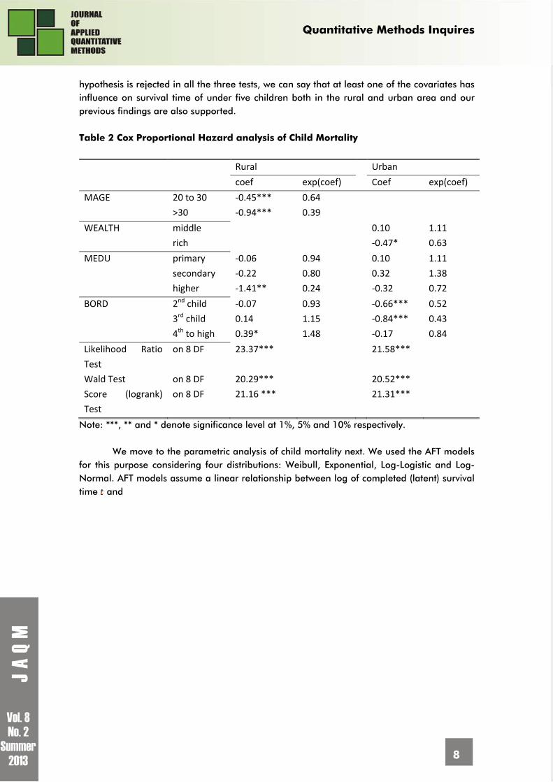
Concluding that all the considered variables both for rural and urban area satisfy the proportionality assumption we moved to Cox-PH analysis of the under five child mortality. Table 2 represents the result obtained from the Cox-PH analysis. Within the Cox model, the best interpretation of for a categorical variable is the hazard ratio. Here, is the hazard ratio for being in the considered group versus the reference group. The factor MAGE came significant for both the considered group (mother’s age between 20 to 30 years and above 30 years)for child mortality compared to the reference group (mother’s age less than 20 years) for rural area. That is,
the estimated hazard ratio (relative risk) of death of children whose mother’s age are between 20 to 30 years relative to children whose mother’s age are under 20 years is 0.64. In other words, children whose mother’s age are in between 20 to 30 years have 36% lower hazard (risk) of death than those children whose mother’s age are under 20 years. The other significant variables can also be interpreted in the same manner. BORD appeared to be a significant factor for child Table 1 Checking Proportionality Assumption
Rural Urban
rho chisq p rho chisq p
MAGE 20 to 30 0.09 0.70 0.40
>30 0.12 1.49 0.22
WEALTH middle 0.06 0.38 0.54
rich ‐0.10 1.18 0.28
MEDU primary 0.03 0.21 0.65 ‐0.02 0.04 0.84
secondary ‐0.02 0.11 0.74 ‐0.08 0.69 0.41
higher ‐0.01 0.02 0.89 ‐0.06 0.35 0.55
BORD 2nd child ‐0.03 0.27 0.60 0.07 0.48 0.49
3rd child 0.02 0.15 0.70 0.07 0.53 0.47
4th to high ‐0.11 3.21 0.07 0.02 0.06 0.81
mortality both for the rural and urban area (though for different group) while WEALTH and MEDU is significant for urban and rural area respectively. The Likelihood ratio test (LRT), Wald test and Score test, test the global null hypothesis that . The global test is analogous to the overall F-test in an Analysis of Variance (ANOVA) or linear regression. It tests whether all of the covariates have no “influence” on survival time. Since the null
Quantitative Methods Inquires
8
hypothesis is rejected in all the three tests, we can say that at least one of the covariates has influence on survival time of under five children both in the rural and urban area and our previous findings are also supported. Table 2 Cox Proportional Hazard analysis of Child Mortality
Rural Urban
coef exp(coef) Coef exp(coef)
MAGE 20 to 30 ‐0.45*** 0.64
>30 ‐0.94*** 0.39
WEALTH middle 0.10 1.11
rich ‐0.47* 0.63
MEDU primary ‐0.06 0.94 0.10 1.11
secondary ‐0.22 0.80 0.32 1.38
higher ‐1.41** 0.24 ‐0.32 0.72
BORD 2nd child ‐0.07 0.93 ‐0.66*** 0.52
3rd child 0.14 1.15 ‐0.84*** 0.43
4th to high 0.39* 1.48 ‐0.17 0.84
Likelihood Ratio
Test
on 8 DF 23.37*** 21.58***
Wald Test on 8 DF 20.29*** 20.52***
Score (logrank)
Test
on 8 DF 21.16 *** 21.31***
Note: ***, ** and * denote significance level at 1%, 5% and 10% respectively.
We move to the parametric analysis of child mortality next. We used the AFT models for this purpose considering four distributions: Weibull, Exponential, Log-Logistic and Log-Normal. AFT models assume a linear relationship between log of completed (latent) survival time and

Quantitative Methods Inquires
9
Table 3 AFT analysis of child mortality
Rural Urban
Weibull Exp Log logistic
Log normal
Weibull Exp Log logistic
Log normal
Intercept 4.71 5.82 4.66 5.15 4.77*** 5.94*** 4.72*** 5.33***
SEX male ‐0.03 ‐0.06 ‐0.03 ‐0.04 ‐0.03 ‐0.06 ‐0.02 ‐0.02
MAGE 20 to 30 0.20 0.34 0.20 0.24 ‐0.01 ‐0.08 ‐0.01 ‐0.07 >30 0.43* 0.79 0.45* 0.55 0.20 0.34 0.21 0.08
MEDU primary 0.05 0.14 0.05 0.10 ‐0.04 ‐0.04 ‐0.04 ‐0.05 secondary 0.14 0.40 0.14 0.17 ‐0.13 ‐0.16 ‐0.13 ‐0.20 higher 0.74 1.70 0.73 0.94 0.18 0.54 0.17 0.17
BORD 1st child 0.04 0.14 0.04 0.05 0.31 0.71 0.32 0.47 2nd child ‐0.50 ‐0.03 ‐0.04 ‐0.00 0.37 0.84 0.38 0.57 4th to high ‐0.17 ‐0.27 ‐0.18 ‐0.21 ‐0.003 0.08 ‐0.01 0.08
WEALTH middle ‐0.01 ‐0.01 ‐0.01 0.03 ‐0.05 ‐0.12 ‐0.05 0.02 rich ‐0.07 ‐0.17 ‐0.07 ‐0.10 0.18 0.36 0.18 0.28
Scale 0.467 1.00 0.457 1.2 0.469 1.00 0.461 1.27
Log (scale)
‐0.76 ***
‐0.78***
0.18**
‐0.76***
‐0.77***
0.24
LogL ‐1773.9 ‐1855.6 ‐1778 ‐1812.9 ‐740.5 ‐773.6 ‐742.3 ‐759.4
LogL (Intercept)
‐1786.1 ‐1867.5 ‐1790.3 ‐1824.9 ‐751.7 ‐785 ‐753.3
‐769.5
Chisq on 11 d.f 24.49 ***
23.9***
24.49***
23.92***
22.45** 22.69** 21.9*** 20.25**
AIC 3573.8 3735.1 3582.0 3651.8 1506.99 1571.22 1510.66 1544.78
Note: ***, ** and * denote significance level at 1%, 5% and 10% respectively. covariate . Now, both for rural and urban area the AIC value is smallest for Weibull distribution indicating Weibull distribution better fits the data than the other distributions. In rural area, only the variable MAGE is significant for greater than 30 years, meaning that for one unit (month) increase in the children’s age, the expected survival time increases by
or 54% more for children whose mother’s age are more than 30 years than children with mother aged less than 20 years. In urban area only the intercept term is significant. The term scale is a time scaling factor, it’s greater than 1 means failure is accelerated (survival time shortened) and vice versa. The Log(scale) is statistically significant relative to 0 and scale is smaller than 1 for Weibull distribution in both areas , indicating failure is decelerated (survival time lengthened).
4 CONCLUSIONS
Using non parametric, semi parametric and parametric approach of survival analysis, this paper investigates the factors that affect the child mortality of children aged under five years in Bangladesh and also compares the child mortality between rural and urban area. The analysis has important implications for the government and non-government organizations and policy makers of the country who deal with child affair and health. The non parametric analysis suggests that in urban area the 4th or higher birth ordered child has a very high failure rate. For both the areas, survival probability is very high for children with higher educated

Quantitative Methods Inquires
10
mother and in urban area the failure rate is very high for children of poor economic status. The Cox-PH regression analysis indicate that in rural area the covariates MAGE, MEDU and BORD have significant affect on child mortality while the significant covariates for urban area are WEALTH and BORD. The AFT analysis shows that for both the areas Weibull distribution better fits the data and only the covariate MAGE is significant for rural area.
REFERENCES 1. Becher, H., Muller, O., Jahn, A., Gbangou, A., Kynast-Wolf, G. and Kouyate, B., “Risk
factors of infant and child mortality in rural Burkina Faso”, Bulletin of the World Health Organization, 82 (4), 2004.
2. Kembo, J. and Ginneken, J.K.V., “Determinants of infant and child mortality in Zimbabwe: Results of multivariate hazard analysis”, Demographic Research, 21, 2009, PP 367-384.
3. Kaplan, E.L. & Meier, P., "Nonparametric estimation from incomplete observations", Journal of the American Statistical Association, 53, 1958, 457-481.
4. Cox, D., “Regression models and life tables”, Journal of the Royal Statistical Society, Series B, 34, 1972, 187-220.
5. Mozumder, ABM. K. A., Khuda, B., Kane, T. T., “Determinants of Infant and Child Mortality in Rural Bangladesh”, International Centre for Diarrhoeal Disease Research, Bangladesh, Working Paper No. 115, 1998.
6. Baqui, A.H., Black, R.E., Arifeen, S. E., Hill, K., Mitra, S.N. and Sabir, A. A., “Causes of childhood deaths in Bangladesh: results of a nationwide verbal autopsy study”, Bulletin of the World Health Organization, 76 (2), 1998, 161-171.
7. Baqui, A.H., A.A. Sabir, N. Begum, S.E. Arifeen, S.N. Mitra, R.E. Black., Causes of childhood deaths in Bangladesh: An update. Acta Paediatr, 90, 2001, 682-690.
8. Bangladesh Demographic and Health Survey. National Institute of Population Research and Training (NIPORT), Mitra and Associates, ORC Macro. Bangladesh Demographic and Health Survey 2007. Dhaka, Bangladesh and Calverton, Maryland: NIPORT, Mitra and Associates and ORC Macro, 2007.
1Nasrin AFZAL - Post graduated in Applied Statistics from Institute of Statistical Research and Training (ISRT), University of Dhaka in 2011. Currently working in International Centre for Diarrhoeal Disease Research, Bangladesh (ICDDR,B) in the research group Human Papilloma Virus and Reproductive Cancer. Got admission with full scholarship in the PhD program in the specialization of statistics in University of Calgary, Alberta, Canada starting from September 01, 2012. Scientific Research Interests: Survival Analysis, Biostatistics, Epidemiology. First author of Papers “An Empirical Analysis of the Relationship between Macroeconomic Variables and Stock Prices in Bangladesh”, Bangladesh Development Studies, Vol. XXXIV, December 2011, No. 4, PP 95-105 and “Determinants and Status of Vaccination in Bangladesh”, Dhaka Univ. J. Sci. 60(1): 47-51, 2012 (January), PP 47-51. 2Sabrina ALAM - Post graduated in Applied Statistics from Institute of Statistical Research and Training (ISRT), University of Dhaka in 2010. Worked in International Centre for Diarrhoeal Disease Research, Bangladesh (ICDDR,B) in the research group Gender, Health, Human Rights and violence against Women. Scientific Research Interests: Survival Analysis, Time Series Analysis, Econometrics.

Quantitative Methods Inquires
11
ON FUZZY REGRESSION ADAPTING
PARTIAL LEAST SQUARES
Catalin Alexandru TANASIE1 PhD Candidate, Doctoral School of Economical Informatics The Bucharest University of Economic Studies, Romania E-mail: [email protected]
Abstract The usage stage of distributed IT&C applications – DIAs raises specific risks relating to the increased processing and usage strain related to live interactions. The incident categories and impact, as well as associated actors, are shown in order to serve as quantifying factors in the building of models aiming at quantifying their impact on distributed application reliability. A model aiming at extension impact assessment is built and details on the evaluation of the MERICS testing application are detailed. The component obsolescence is evaluated through an additional model and its impact on MERICS is shown alongside difficulties in identifying composing factors. Key words: distributed applications, interdependencies, MERICS, users, processes
1. DIAs internal and external interdependencies
The interactions that describe DIA usage are controlled by authentication and
authorization mechanisms that establish user identity and assign him with component or method-based access rights that enable the separation and differentiation of information control, with benefits to overall application security and data integrity. The following user role types are identified:
functional user roles, associated to persons or processes that act in performing storage and computations on information as specified in the application’s operational scenarios and defining the extent of operational method and data access, as well as managing content through differentiated query, insert, update and delete function access at database and table level, as well as associated read, write and delete file access rights; MERICS differentiates between the loading of images and video content and its review or testing with subsequent method access-driven, authorization-differentiated graphical interfaces through-out the presentation layer; analytic user roles, designed to manage authorized access to meta-information related to the functional domain in DIA usage - data mining, reports, building analytical structures such as OLAP cubes and reviewing results; MERICS defines analytical roles for both the definition and structuring of reporting based on input gathered by risk assessment functions and tools; they do not include access to

Quantitative Methods Inquires
12
predefined reports that target unrefined operational data, leaving this prerogative to the functional roles; technical user roles, tasked with intermediating access to context and maintenance-related functions and tools as part of the distributed application components and deployment environment; administrators and operators interact with supporting DIA technologies in order to improve on performance, maintain the functioning status of the system and intermediate security tasks – including the creation and updating of user roles; MERICS is managed internally by the author and externally by the hosting service provider.
Defining security roles is done considering the user activity domain as related to DIA
design and implementation specifications, which in turn determines the following categories and associated risks in table 1:
Table 1. Role-determined security risks
Name Area Description Effects Countermeasures Excessive access granting
F overextending user role access, appending existing credential rights instead of creating specialized new ones
data loss or unauthorized and unmanaged changes
new roles for new operational and data access combinations
Insufficient access granting
F access restriction relies only on security criteria rather than including operational ones
DIA usage flexibility decrease, impossibility of finishing tasks
using user groups and encryption-based authentication mechanisms for sensitive areas
Improper use case mapping
F failure in understanding security and operational requirements
communication and data quality loss
security role analysis and periodic reviews
Operational access
A availability of altering mechanisms for the operational information that constitutes the basis for analysis
analytical output relevance loss, loss of operational information privacy
building automated information gathering and processing mechanisms
Undifferentiated analytical review access
A insufficient delimiting in analytical information security implementation
privacy loss, productivity decrease through the building and usage of irrelevant reports in specific usage areas
classification of report security and information content loss effects
Technical personnel access
T access to confidential operational and analytical information by virtue of technical skills and tools
information loss or altering
backup, auditing, delegation and separation of technical responsibilities
Unverified maintenance tasks
T badly scheduled or un-reviewed maintenance jobs and actions on deployment tools and DIA components
interference with operational and analytical tasks, delays, data loss, unauthorized access
scheduling of maintenance, operational and analytical processes, documenting procedures

Quantitative Methods Inquires
13
The F,A and T areas identify the functional, analytical or technical roles that constitute the risk source.
User responsibilities derive from roles by the addition of direct correspondence to operational use cases and the structure of the group or organization using the distributed application. They correspond to a mapping of the hierarchical structure of the organization and application usage roles, as defined in figure 1 and the following generic model describing their composition.
Let set define the hierarchical structure of the users and persons that interact with the input or output of DIA components as specified by the functional use cases and described by
and set of items that define the roles associated to the usage of the distributed
application components in the performing of tasks:
The access to information and operations derived from the function and specifics of
the position an employee or contributor has and its relation to neighboring nodes in the tree-like structure formed by describing these associations. Responsibilities define direct and indirect access and implicit influence of an actor on the content and form of the information operated upon by the system.
Let be the set of roles mapped to node , as determined by the specifics of
operations performed. The responsibility of the associated user hierarchical position does not limit itself to these, but includes the ones belonging to underlying hierarchical positions, defined by set defining relating roles:
where:
– number of associated roles for node ;
– roles associated directly to node and corresponding to items in set .

Quantitative Methods Inquires
14
Figure 1. Organization hierarchy – application roles correspondence Based on the previous model and information in figure 1, responsibilities for position
node , corresponding to user 3 has the following values assigned:
detailed as
uc Data Model
Application RolesOrganization
H_1
H_2H_3
H_5 H_4 H_7 H_6
H_k
H_8 R_1
R_2
R_3
R_l
R_m
H_n

Quantitative Methods Inquires
15
As observed, even if user 3 has no direct role associated, he inherits from the relationship defined by links in the DIA hierarchy. The assignment of responsibilities introduces the problematic of defining and delimiting hierarchical positions and associated workloads, in order to correctly map roles to operational and analytical functions.
Distributed application components are separated by platform, role, physical location and security concerns in sections which interact within platforms and communication media shared by multiple systems. The reliance on common information structures and messaging channels impacts on the performance and availability of methods and creates the need for assessing the impact of incidents and improperly functioning platform components in the performance of the application. The interdependency property, defined as the degree in which the operational status and output of a component influences the activity of another.
Internal interdependencies characterize DIA modules and tools within the same application, relating to communication, synchronous and asynchronous operation, security and incident effects, as well as the impact of damaged or invalid information in the functioning and output relevance for later usage. MERICS introduces dependencies of different magnitude as the architectural layer increases, with persistence isolated and secured from synchronicity or damage propagation as compared with the service or presentation layers.
External interdependencies define interactions with outside modules, across communication channels whose traffic is not under the supervision of the DIA operating parties and are accessible to a various degree to the general public. In addition, it includes the aspect of deployment platform failures or hardware performance as a factor that affects the functioning of components. MERICS, the distributed application used as a testing platform in risk factors identification, as well as risk assessment model evaluation, relies on the deployment platform specifics – hardware, software instruments – in the overall performance, with impact on the timing of synchronous methods and susceptibility to security threats.
The items shown in tables 2, 3 and 4 are selected to reflect on their importance in the usage of distributed applications, alongside a description of effects, counteractions and the practical implementation of these, numbered as follows: MERICS.TEST.Desktop (1), MERICS.WEBAPP (2), MERICS.LOGICAL (3), MERICS.OPERATIONAL (4), MERICS.COMMON (5), MERICS.DataOperations (6), MERICS.AUTHENTICATION (7), MERICS.WCF (8), MERICS.Service (9), MERICS.ANALYTICAL (10) and MERICS.CONTEXT (11), as well as the operational (12) and analytical (13) databases.
The communication channels represent a vulnerable component of distributed applications through their susceptibility to attacks and the unavailability of details relating to their operating status and performance. The information transferred across them undergoes two separate and complementary processes, as formats in emitter and receiver entities are aligned and security-enhancing procedures are performed. Table 2 details on the risks that induce lower operating quality and increase the time needed to process requests.

Quantitative Methods Inquires
16
Table 2. Communication risks Risk Description Effects Counteractions ME
RICS
Unsynchronized data contracts usage
outdated WSDLs, failure to communicate changes, changes in the optional status of method arguments
errors, incomplete parsing of information, deprecated methods and attributes usage
documenting and communicating changes on the emitter side, periodic validation of message format on the receiver side; usually appears in public, general-use Web services – weather, exchange rates
(5), (8), (9)
Improper type formatting
changes in encoding, length, content appearing in formatting and encoding or decoding
data loss errors, loss of information quality, delays due to recasting
validating hardware and software compatibility in communication actors
(8), (9)
Incompatible complex structure usage
using custom-built structures that rely on incompatible data types or which are not described by data contracts
errors and information loss due to decoding failure
including complex type definition and encoding in service description files
(5), (8), (9)
Variances in endpoint security
changes in security levels through-out the communication components
security validation errors, authentication failures
assessing the impact of unilaterally increasing or decreasing security
(7), (8), (9)
Message delays time-outs in receiver communication endpoints
errors and delays in task processing, loading of memory for queued messages
asynchronous methods, alternate, interchangeable role modules
(3), (4), (8), (9)
The nature of DIA component interactions is a factor in the measuring of incident
susceptibility, as the context of their operations raises risks with respect to data quality, module availability and processing load. The interaction between components and dependency on timed actions constitutes a criterion in the definition of asynchronous and synchronous operations.
Asynchronous processes, shown in figure 2, bottom section, operate on information without having to relate on external output in the finishing of tasks. Data formatting, as well as scheduled jobs in operational and analytical databases belong to this category. In the course of their execution, they do not require or rely on data changes triggered by other components. They are less susceptible to errors relating to informational quality or validation than their counterparts. MERICS implements asynchronous operations primarily at database level, as the formatting and export of operational database records for data mining purposes

Quantitative Methods Inquires
17
is a primarily technical task done without regard to the quantity or content of information, within predetermined specifications and using known filters. All input information is known at the moment of execution. If processes communicate, response information is used outside the context of the task.
Figure 2. Synchronous and asynchronous processes Synchronously operating processes, shown in figure 2, top section, depend on others
in the solving of tasks, and whose output is affected by the order of interactions and are susceptible to incidents that derive from the timing and information dependencies in these steps. Not all information is known a priori, as opposed to the other category, with consequences on the order and timing of steps. Table 3 identifies the incidents that synchronous operations involve, as well as the MERICS components implementing countermeasures.
act Data Model
Pro
cess
BP
roce
ss A
Pro
cess
BP
roce
ss A Start
Syncronous Operation
Compose requestSend Request
Receive task
Start Listen channel
Messagereceived?
Synch
Notify reception
Process
Send output
Listen channel
Receive answer
Requestanswered?
Asynchronous Operation
Process task
End
Compose request
Start
Send Request
Receive task
Start Listen channel
Messagereceived?
Process
Send output
End
Process task
Listen channel EndContext-independent
action
MessageReceived?
Receive answer
End
No Yes
No
No Yes
No Yes

Quantitative Methods Inquires
18
Table 3. Synchronous process incidents Incident Description Effects Counteractions MERI
CS
Time-outs and component unavailability
failure in receiving the answer within a given period, either arbitrarily chosen or predetermined
outcome quality and availability
alternate services, extending time-out intervals
(3), (4), (8), (9)
Excessive request strain
overloading of a component’s capabilities by request number
delays in processing requests, errors in emitter and sender components
extending hardware capabilities, adding similar components, load balancing software controllers
(3), (4), (10), (11)
Cascade effect propagation
delay time builds up as multiple components are affected
in services that share communication channels and message queues, unrelated incidents cause failures in properly functioning exchanges
using multiple communication channels for critical tasks, prioritizing and excluding underperforming items from the queue
(3), (8), (9), (11)
Brute force limitations in timing increase attacks damage
unavailability of communication
Implementing communication pattern detectors and additional service components
(7), (8), (9)
Impersonation limits in response time and available security protocols increase the likelihood of successful security breaches
data theft and altering due to failures in detecting attacks over small periods of time
Using pattern detectors, switching to asynchronous messaging in data whose exchange is not time-critical
(7), (11), (10)
Autonomy is the DIA component level correspondent of asynchronous processes,
defining modules that act independently of the status and informational content of other runtime components, relying on input information that is already present within the system. However, this feature does not exclude vulnerabilities deriving from the quality of both input and output data, as other processes influence the relevancy of results. Additionally, autonomy is not required to be mutual, as DIA usage includes scenarios in which these components serve as real-time input providers for others, often within synchronous jobs. Table 4 details on vulnerabilities, effects and MERICS components implementing software features minimizing impact on the application.

Quantitative Methods Inquires
19
Table 4. Autonomous component vulnerabilities Vulnerability
Description Effects Counteractions MERICS
Data relevancy
unavailability of real-time quality checks
storage and processing of improperly validated information
implementing validation controls in both input and output information
(1),(2),(4), (6),(12), (13)
Incident communication
failures are not detected instantly by other components in the system
reliance on improperly functioning components
implementing auditing and fault detectors
(7),(8),(9), (11),(12), (13)
Specialization autonomous components act in predetermined, inflexible process areas with a high degree of specialization
limited reliance on autonomy as protection against errors and security threats
extending impact by implementing asynchronous computation tasks in autonomous components
(3),(4)
Error detection
data loss and altering is not immediately detected outside autonomously operating components
improperly formatted, invalid information in interdependent components that process information at a later time
synchronous fault detectors, validation in all interacting components
(1),(2), (3),(4), (9),(11)
Improper maintenance
improper functioning is not readily understood or detected by maintenance crew
derived from the high specialization, it affects component and process availability
documentation, training, separation of tasks within technical usage areas
(3)
Information flow in DIA-mediated tasks is dependent on the synchronization of
components and availability of input for each successive step in computation. The specialization of DIA modules, beneficial to the speed and quality of output, increases incident risks due to the dependencies it imposes, as the system components do not posses all available information and algorithms to provide answers, relying on collaboration to achieve the completion of jobs. Considering this property, deficiencies in information synchronization include:
reduced contextual awareness in multi-system collaboration; the users of an application are performing specific tasks, and may not be completely aware of the relevancy and global positioning of the specific stage they mediate, leading to decreased information quality as the input is not contextually validated and security vulnerabilities by the failure to protect data as its sensitivity is unknown;
information quality deficiencies, as collaborating components rely on previous stages in validating information and take its correctness for granted; an algorithm for assessing component performance is limited to factors inside the analyzed methods; in MERICS this feature created problems in both operational and analytical modules, as the need quality of output is dependent on the entirety of actions performed as part of an use case; adding validation controls

Quantitative Methods Inquires
20
and cross-system analytical factors reduces the incidence of incorrect information processing.
2. DIA maintenance risks
Maintenance relates to the manual tasks and processes that serve the optimum
functioning of DIA components and communication channels. It is performed by technical users, administrators and external parties, as well as by means of automated repository and memory cleansing, message flow refining, load balancing and caching operations. It contains two separate areas of interest as relating to the target of the jobs performed – hardware and software.
Hardware maintenance groups together actions that aim at the updating and ensuring a proper running state for devices on the DIA deployment platform. Considering risks developed as part of the maintenance processes, hardware management targets the avoidance or minimization of:
power failures, with energy backup systems and recovery monitoring; the purpose of installing alternative generators ranges from ensuring an interval for saving session and operational information before performing a controlled shutdown, in the lower extreme, to the indefinite ensuring of the power supply in a transparent transition that does not affect user activity;
hardware component failures, with repair or replacement options in situations where recovery is impossible; servicing, intermediate backup systems, multiple interacting units similar to parallel processing ensure the minimization of incident effects; documenting on recovery procedures and communicating vulnerabilities, as well as tracing the source of the incidents helps reduce the inherent component downtime or increased strain on similar ones in DIA usage;
data loss – potentially damaging to the relevancy and availability of information, it relates to failures in storage instruments – hard-disks, backup tapes, mobile devices; prevention through backup and the subsequent maintenance of versions and copies by specialized companies or through internal resources, recovery procedures for damaged disks, fire prevention for storage rooms, ensures the lowering of costs induced by missing or irrecoverable information; the budget for such procedures varies depending on the activities that distributed applications manage;
security – brute force attacks, unauthorized access, data handling leaves traces in the hardware components runtime indicators – power usage, temperature, sound; AES encryption information is gathered by means of viewing patterns in electrical voltage as blocks of data are encrypted every nine steps and every cipher item leaves a distinct signature – figure 2 lower section, with the attacker able to identify specific patterns and gradually identifying components through successive trials; in a similar fashion, maintenance operators and processes trace the hardware signature of attacks as part of routine component status surveillance – figure 2, upper section (1).

Quantitative Methods Inquires
21
Figure 3. AES encryption algorithm attack hardware signature (1)
Figure 4. DIA performance dependencies
uc DIA Performance
DEPLOYMENT CONTEXT
USERS
APPLICATION
DIA Performance
Process synchronization
Message encryption
Operation security
Hardware resources
Component number
Operating system
Software framework
Authentication
Authorization
Interfaces Administration
Load balancing
Quantitative Methods Inquires
22
Information is exchanged between DIA components by means of messaging
conduits, formatting and encrypting data at one end, as well as validating credentials and recomposing the programmatic entities at the other. These operations are influenced by user access and the operational status of the channels and endpoints. In concurrent, multiple source DIA interactions, credentials and message content serve as prioritizing factors, as well as the first layer of defense against security breaches. Maintenance tasks relate to the management of:
user credentials, as over the lifespan of the application the identities of the accessing persons and processes change, as well as the validity of input – passwords and digital certificates expire, users move inside and outside the DIA-operating organization, component security requirements change with the diminishing or increasing of risk factors for specific tasks; maintenance technicians and scheduled processes ensure the periodic updating of database and operating system access, especially in user accounts with administrative or confidential clearance;
message queuing review and configuration, with surveillance of channel load, incidents and configuration of bandwidth for the insurance of efficient and time-efficient communication, especially with respect to synchronous processes; prioritizing messages and incidents based on severity scales configurable through administrative interfaces; the MERICS.CONTROL module delegates tasks acting in part based on preconfigured component and message priority, with the possibility of runtime reevaluation.
The direction of the dependency indicators in figure 4 as opposed to the context also indicates the coverage area of the effect, with inward referencing arrows indicating specificity to the described process, and outward the generalness of the property. Considering a graph representation of the interactions, the roads between nodes indicate the chain of dependencies; the software framework, as described in the approach, impacts DIA performance in two ways – directly, through processing support, protocols and standards, and indirectly, by influencing and being influenced by the operating system, which in turn defines the hardware resources usage and indirectly the maximum component number, with direct effect on DIA performance.
The performance of distributed application components is affected by risks deriving from vulnerabilities and interfering in successive layers as related to the usage environment, shown in figure 3:
the deployment context, associating hardware and software support components as well as the technologies that form the basis of the application runtime execution; operating systems and software framework choices affect each other and the system’s performance; MERICS uses cross-platform Microsoft technologies, with the optimization of their interaction relevant in isolating external interference in determining operational and assessment model behavior;
the usage context, with authentication and authorization, as well as operational administration and interface design impacting on the amount of resources used by DIA modules; the security level, encryption protocols and number of external interactions affect the performance and computing efficiency; MERICS separates

Quantitative Methods Inquires
23
the endpoints based on the risk assessment values, with effects in the optimization of resource sharing;
the application, with component number, process control, security and encryption algorithms implementation influencing the amount of computation power needed for usage; MERICS implements operational control, multi-threading, task separation and ordering, as and analytical evaluation of performance indicators, with continuous optimization for underperforming algorithms.
CONCLUSIONS Incident prevention ensures the minimization of frequency of occurrence, as well as
the cost of recovery and revision of application components. In situations where prevention fails or is not envisioned and incidents occur, assessment and recovery protocols ensure the lowering of damage done through direct and indirect costs. Table 5 identifies the steps as envisioned during the development and usage of the MERICS distributed application.
Table 5. Disaster recovery steps
No. Step Issues Actors
1 Identification determining the source, security break, affected components
operational users, developers, maintenance crew, system administrators
2 Stopping of malicious activity
action effectiveness, difficulties in eliminating all attack routes
administrators, operational users
3 Removal of damage restarting affected components, recovering lost or tampered information
functional and database administrators, operators
4 Behavior description area of incidence, technical or logical vulnerability
users, business analysts, system designers, developers, testers
5 Assessment of effects choosing assessment models, risk budgeting, cost valuation
users, operational management,
6 Application updating extending functionalities in affected components, improving security algorithms and procedures
system and security designers, developers
7 Testing validating changes, reproducing incident scenarios
developers, testers, users
8 Deployment replacing faulty components in the live usage environment
Functional administrators, testers, users
9 Documentation Evaluating impact and documenting effects, patterns of occurrence and response
users, business analysts, designers, developers, testers, management
The completion of first three steps of the procedure defines the cost impact of the incident, as the timing and tools available in detecting and counteracting threats and failures in the application’s components influence their span and effects.

Quantitative Methods Inquires
24
The damage removal stage in disaster recovery procedures includes the resubmitting and reprocessing of pending requests and tasks at the moment of incident occurrence. Factors in the prioritizing of jobs derive from the following aspects:
the severity of the request in what concerns the importance of output delivery speed in the quality of the response; real-time information such as exchange rates and stock exchange quotations lose their relevance over small periods and must be processed by alternate modules; MERICS prioritizes information exchange through the usage of its control role component, as well as reevaluation of the delegation mechanisms through input from MERICS.ANALYTICAL and associated database;
the identification of erroneous messages following the same pattern that caused the error, if the structure or content of the communication was the source of the vulnerability, as well as the identification of security threats related to security incidents, in case the attacker forces his entry into the system by more than one communication item.
The reprocessing capacity of the system is improved by the implementation of role-interchanging components, which are available for task delegation in case the functionality of one module is disturbed.
References2 1. Adams, C., Farrell, S.; Internet X.509 Public Key Infrastructure: Certificate Management
Protocols, Network Working Group, March 1999, http://tools.ietf.org/html/rfc2510 2. Konstantinos Markantonakis, Michael Tunstall, Gerhard Hancke, Ioannis Askoxylakis, Keith Mayes –
Attacking smart card systems: Theory and practice, Information Security Technical Report, Nr. 14, 2009, pg. 46 – 56, ISSN: 1363-4127
3. Nagpal, R.; Simple guide to digital signatures, Asian school of cyber laws, 2008, www.asclonline.com
4. Nissanke, N.; An integrated security model for component-based systems, Emerging Technologies and Factory Automation, 2007 ETFA IEEE Conference on Emerging Technologies and Factory Automation, pp. 638 – 645, ISBN 978-1-4244-0825-2
5. Tilborg, Henk C.A. van; Jajodia, Sushil, Encyclopedia of Cryptography and Security, 2nd edition, 2011, Springer Reference, 1435 pp., ISBN 978-1-4419-5905-8
1 Catalin Alexandru TANASIE is a graduate of the Faculty of Cybernetics, Statistics and Economic Informatics within the Bucharest University of Economic Studies, the Economic Informatics specialization, 2007 promotion. Starting the same year he attended the Informatics Security Master in the same institution, and is currently a PhD student at the Doctoral School within the Bucharest University of Economic Studies. He has concerns in the field of distributed applications programming, evolutionary algorithms development, part of the field of artificial intelligence - neural and genetic programming. Currently he works as an application designer in a financial institution, in areas concering the development of commercial applications. 2 Codification of references in text:
[1] Konstantinos Markantonakis, Michael Tunstall, Gerhard Hancke, Ioannis Askoxylakis, Keith Mayes – Attacking smart card systems: Theory and practice, Information Security Technical Report, Nr. 14, 2009, pg. 46 – 56, ISSN: 1363-4127
[2] Adams, C., Farrell, S.; Internet X.509 Public Key Infrastructure: Certificate Management Protocols, Network Working Group, March 1999, http://tools.ietf.org/html/rfc2510
[3] Nagpal, R.; Simple guide to digital signatures, Asian school of cyber laws, 2008, www.asclonline.com
[4] Nissanke, N.; An integrated security model for component-based systems, Emerging Technologies and Factory Automation, 2007 ETFA IEEE Conference on Emerging Technologies and Factory Automation, pp. 638 – 645, ISBN 978-1-4244-0825-2
[5] Tilborg, Henk C.A. van; Jajodia, Sushil, Encyclopedia of Cryptography and Security, 2nd edition, 2011, Springer Reference, 1435 pp., ISBN 978-1-4419-5905-8

Quantitative Methods Inquires
25
A STEP-WISE METHOD FOR EVALUATION OF DIFFERENTIAL ITEM FUNCTIONING
Muhammad Naveed KHALID University of Cambridge ESOL Examinations, UK E-mail: [email protected]
Cees A. W. GLAS PhD, University Professor, Department of Research Methodology, Measurement and Data Analysis Faculty of Behavioral Science, University of Twente, Netherlands E-mail: [email protected]
Abstract: Item bias or differential item functioning (DIF) has an important impact on the fairness of psychological and educational testing. In this paper, DIF is seen as a lack of fit to an item response (IRT) model. Inferences about the presence and importance of DIF require a process of so-called test purification where items with DIF are identified using statistical tests and DIF is modeled using group-specific item parameters. In the present study, DIF is identified using item-oriented Lagrange multiplier statistics. The first problem addressed is that the dependence of these statistics might cause problems in the presence of a relatively large number DIF items. A stepwise procedure is proposed where DIF items are identified one or two at a time. Simulation studies are presented to illustrate the power and Type I error rate of the procedure. The second problem pertains to the importance of DIF, i.e., the effect size, and related problem of defining a stopping rule for the searching procedure for DIF. The estimate of the difference between the means and variances of the ability distributions of the studied groups of respondents is used as an effect size and the purification procedure is stopped when the change in this effect size becomes negligible. Key words: Differential Item Functioning; Effect Size; Item Response Theory; Model Fit; Polytomous Items
INTRODUCTION
Differential item functioning (DIF) occurs when respondents with the same ability but from different groups (say, gender or ethnicity groups) have a different response probabilities on an item of a test or questionnaire (Embretson & Reise, 2000). Several statistical DIF detection methods have emerged in the last three decades (Camilli, 1992; Dorans & Kulick 1986; Finch, 2005; Holland & Thayer, 1988; Kelderman & Macready, 1990; Lord, 1980; Muthén, 1988; Shealy & Stout, 1993; Swaminathan & Rogers, 1990; Thissen, Steinberg, & Wainer, 1988; Raju, 1988; Roussos & Stout, 1996). During this period many researchers have reviewed various DIF detection methods (e.g., Camilli & Shepard, 1994; Holland & Wainer, 1993; Millsap & Everson, 1993; Penfield & Camilli, 2007; Roussos &

Quantitative Methods Inquires
26
Stout, 2004). Most of the techniques proposed for the detection of DIF have been based on the evaluation of differences in response probabilities between groups conditional on some measure of ability. We can classify these techniques under two general categories: the first category is where a manifest score, such as the number-correct score, is taken as a proxy for ability and the second is where a latent ability variable of an IRT model functions as an ability measure. The most common method used in the first category is the Mantel-Haenszel (MH) approach where DIF is evaluated by testing whether the response probability, given number-correct scores, differs between the groups. The MH test works quite well in practice under the Rasch model. Fischer (1993, 1995), however, argues that its application under other IRT models raises several theoretical limitations. For instance, sufficient statistics does not hold for the 2PL and 3PL models. Fischer’s view on sufficient statistics equally applies to the log-linear approach where sum scores are used as proxies for ability; this view is also shared by Meredith and Millsap (1992). The observed score is nonlinearly related to the latent ability metric (Embretson & Reise, 2000; Lord, 1980) and factors such as guessing may preclude an adequate representation of the probability of correct response conditional on ability. Having said that, in general the correlation between the number-correct scores and ability estimates is quite high, so this is not the most important reason for considering alternative methods. The main problem arises in situations where the number-correct score loses its value as a proxy for ability. For example, there are test situations with large amounts of missing data and in the case of computer adaptive testing, where every student is administered a virtually unique set of items. In all these situations the number-correct score may not be appropriate for a meaningful assessment.
In an IRT model, ability is represented by latent variable θ, and a possible solution to the number correct score problem is to apply the MH and log-linear approach using subgroups that are homogenous with respect to an estimate of θ. This, however, introduces a different problem that the estimate of θ is subject to estimation error, which is difficult to take into account when forming the subgroups. An alternative is to view DIF as a special case of misfit of an IRT model and to use the machinery for IRT model-fit evaluation to explore DIF. An overview of this approach was given by Thissen, Steinberg, and Wainer (1993). In that overview, evaluation of item parameter invariance over subgroups using Likelihood ratio and Wald statistics was presented as the main statistical tool for detection of DIF. Glas (1998, 1999) argues that the Likelihood ratio and Wald approach are not very efficient because they require estimation of the parameters of the IRT model under the alternative hypothesis of DIF for every single item. To address these shortcomings, Glas (1998, 1999) proposes using the Lagrange multiplier (LM) test by Aitchison and Silvey (1958), and the equivalent efficient-score test (Rao, 1948), which do not require estimation of the parameters of the alternative model. Further, this approach supports the evaluation of many more model assumptions such as the form of the response function, unidimensionality and local stochastic independence, both at the level of items (Glas & Falcón, 2003) and at the level of persons (Glas & Dagohoy, 2007).
All methods listed above are seriously affected by the presence of high proportions of DIF items in a test and by the inclusion of DIF items in matching variable. To address this issue, several scale purification procedures have been suggested for the DIF detection methods, such as the two-stage or iterative Mantel-Haenszel method (Holland & Thayer, 1988), the iterative Mantel method, the iterative generalized Mantel-Haenszel method

Quantitative Methods Inquires
27
(Wang & Su, 2004a, 2004b), the iterative logistic regression method (French & Maller, 2007), and the iterative linking IRT-based method (Candell & Drasgow, 1988; Park & Lautenschlager, 1990).
Scale purification procedures are useful in maintaining Type I error rate and have high power when tests contain only a few DIF items. However, if tests have many DIF items, then DIF contamination cannot be completely eliminated by current scale purification procedures. Similar conclusions have been drawn when scale purification procedures were implemented on IRT-based DIF methods (Candell & Drasgow, 1988; Lautenschlager, Flaherty, & Park, 1994; Park & Lautenschlager, 1990) and non-IRT-based DIF methods (Clauser, Mazor, & Hambleton, 1993; French & Maller, 2007; Hidalgo-Montesinos & Gómez-Benito, 2003; Holland & Thayer, 1988; Miller & Oshima, 1992; Navas-Ara & Gómez-Benito, 2002; Wang & Su, 2004a, 2004b, 2010). In this paper we propose an alternative scale purification method using Lagrange multiplier tests to address DIF contamination.
The significance of DIF, the extent to which the inferences made using test results are biased by DIF, is yet another important issue that needs to be looked at. The effect size of DIF is important to consider to avoid complicating inferences by practically trivial but statistically significant results. An example of a method to quantify the effect size is the DIF classification system for use with the MH statistical method developed by the Educational Testing Service (Camilli & Shepard, 1994; Clauser & Mazor, 1998). In an IRT framework we propose to use an estimate of the difference between the means of the ability distributions of the studied groups of respondents as an effect size. This is motivated by the fact that ability distributions play an important role in most inferences made using IRT, such as in making pass/fail decisions, test equating, and the estimation of linear regression models on ability parameters as used in large scale education surveys such as NEAP, TIMSS and PISA.
In this paper we would first sketch a model of DIF and a concise framework of Lagrange multiplier test for the identification of DIF items. We would then present a number of simulation studies of the Type I error rate and power analysis. The difference between two versions of the LM test, one targeted at uniform DIF and one targeted at non-uniform DIF will be shown using a simulated example. This is followed by presenting an example using empirical data to show how the procedure works in practice. Finally, some conclusions are drawn, and suggestions for further research are provided.
DETECTION AND MODELING OF DIF
In IRT models, the influences of items and persons on the observed responses are modeled by different sets of parameters. Since DIF is defined as the occurrence of differences in expected scores conditional on ability, IRT modeling seems especially fit for dealing with this problem. In practice, more than one DIF item may be present and therefore a stepwise procedure will be proposed where DIF items are identified one or two at a time. Both the significance of the test statistics and the impact of DIF are taken into account. The following procedure will be used here for detection and modeling of DIF. First, marginal maximum likelihood (MML) estimates of the item parameters and the means and variance parameters of the different groups of respondents are made using all items. Then an item is identified with the largest significant value on a Lagrange multiplier (LM) test statistic targeted at DIF. To model the DIF in this item, the item is given group-specific item

Quantitative Methods Inquires
28
parameters. That is, in the analysis, the item is split into two virtual items, one that is supposed to be given to the focal group and one that is supposed to be given to the reference group. Then, new MML estimates are made and the impact of DIF in terms of the change in the means and variances of the ability distributions is evaluated. If this change is considered substantial, the next item with DIF is searched for. The process is repeated until no more significant or relevant DIF is found. The assumptions of this procedure are that (1) the item which is mostly affected by DIF will have the largest value of the LM statistic regardless of the bias caused by the other items with DIF, and (2) the change in the means and variances of ability distributions will decrease when the items with the DIF are given group specific item parameters one or two at a time. IRT Models
In the present study, we both consider dichotomously and polytomously scored items. For dichotomously scored items, the one-parameter logistic model (1PLM) by Rasch (1960), the two-parameter logistic model (2PLM) and the three-parameter logistic model (3PLM) by Birnbaum (1968) will be used. For polytomously scored items, we use the generalized partial credit model (GPCM, Muraki, 1992). However, the methods proposed here also apply to other models for polytomously scored items, such as the PCM by Masters (1982) or the nominal response model by Bock (1972).
In the 3PLM, the item is characterized by a difficulty parameter i , a discrimination
parameter i and a guessing parameter i . Further, θn is the latent ability parameter of
respondent n. The probability of correctly answering an item (denoted by X 1ni ) is given
by
exp( ( ))
( X 1 | ) ( ) (1 ) .1 exp( ( ))ni n i i
i n ii n
i n i
P P
(1)
If the guessing parameter i is constrained to zero, the model reduces to the 2PLM
and if the discrimination parameter i is also constrained to one, the model reduces to the
1PLM. DIF pertains to different response probabilities in different groups. Here we consider
two groups labeled the reference group and the focal group. The generalization to more than two groups is straightforward. A background variable will be defined by
1 if person n belongs to the focal group,
0 if person n belongs to the reference group.ny
As a generalization of the model defined by equation 1 we consider
exp( ( ) ( ( )))
( ) (1 ) .1 exp( ( ) ( ( )))i i
i n i n i n ii n
i n i n i n i
yP
y
(2)
This model implies that the responses of the reference population are properly
described by the model given by equation 1, but that the responses of the focal population
Quantitative Methods Inquires
29
need additional location parameters i , additional discrimination parameters i , or both as
given by equation 2. The first instance covers so-called uniform DIF, that is, a shift of the item response curve for the focal population, while the later two cases are often labeled non-uniform DIF, that is, the item response curve for the focal population is not only shifted, but it also intersects the item response curve of the reference population.
For polytomous items, the GPCM by Muraki (1992) will be used. The probability of a
student n scoring in category j on item i (denoted by X 1nij ) is given by
1
exp( )( X 1 | ) ( ) ,
1 exp( )i
i n ijnij n ij n M
i n ihh
jP P
h
(3)
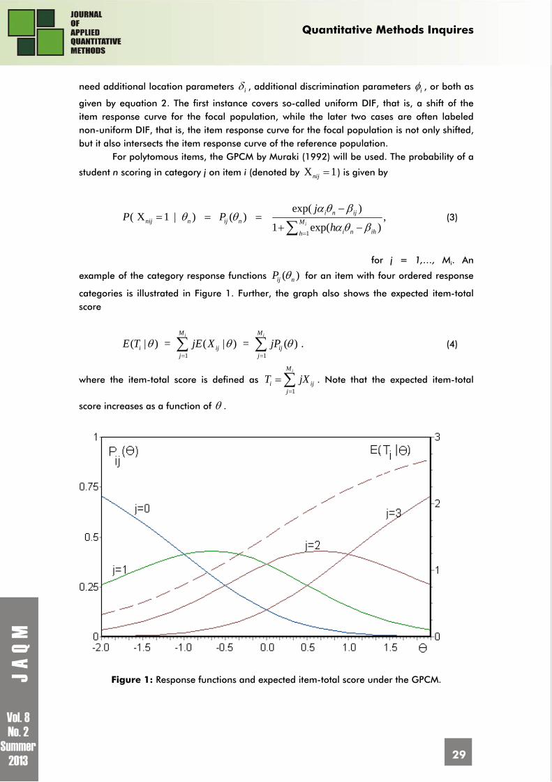
for j = 1,…, Mi. An
example of the category response functions ( ) ij nP for an item with four ordered response
categories is illustrated in Figure 1. Further, the graph also shows the expected item-total score
1 1
( | ) = ( | ) = ( ) .i iM M
i ij ijj j
E T jE X jP (4)
where the item-total score is defined as 1
iM
i ijj
T jX
. Note that the expected item-total
score increases as a function of .
Figure 1: Response functions and expected item-total score under the GPCM.

Quantitative Methods Inquires
30
MML Estimation The LM test for DIF will be implemented in an MML estimation framework. To
describe the statistic, MML estimation will be outlined first. MML estimation was developed
by Bock and Aitkin (1981; see also Bock & Zimowski, 1997; Mislevy, 1984, 1986; Rigdon &
Tsutakawa, 1983). In the MML framework adopted here, it is assumed that the respondents
belong to groups, and that ability parameters of the respondents within a group have a
normal distribution indexed by a group specific-mean and variance parameter. Let
( )( ; )n y ng λ be the density of ability distribution of group y, with parameters ( )y nλ where
y(n) = yn, i.e., the index of the group to which respondent n belongs. To identify the model,
the mean and variance of one of the groups are usually set to zero and unity, respectively.
Further, let ξ be a vector that contains all the item parameters. Finally, η is the vector of all
item parameters ξ and the parameters λ of the ability distributions. The log likelihood
function of η can be written as
( )1
) log ( | , ) ( ; ) .log (N
n n y nn
n np g dL
η x ξ λ (5)
where ( | , )n np x ξ is the probability of response pattern xn of respondent n (n = 1,…, N).
The estimation equations that maximize the log-likelihood are found by setting the first-order derivatives of equation 5 with respect to η equal to zero. Glas (1999) shows that expressions for the first-order derivatives can be derived using Fischer’s identity (Efron, 1977; Louis, 1982):
log ( ) ( ) | ;n nn
L E
η η xη
(6)
with
( )( ) log ( | , ) ( ; )n n n y nnp g η x ξ
ηλ
The expectation in equation 6 is with respect to the posterior
distribution ( )( | ; , )n n y np x ξ . That is, the first order derivatives are equal to the posterior
expectations of the first order derivatives of a likelihood function where the ability parameters are treated as observations. This grossly simplifies the derivations of the
likelihood equations because ( )n η is very simple to derive. As an example we derive the
MML estimate for the mean of the ability distribution of the focal group, that is, the group of respondents where yn = 1. The distribution of the ability parameters is normal, so if the
values of n would be known, the estimation equation ( ) 0nn
η would be equivalent to
1
1
.
N
n nnN
nn
y
y

Quantitative Methods Inquires
31
By Fisher’s identity as given in equation 6, the MML estimation equation becomes
1
1
| ; .
N
n n nnN
nn
y E
y
x (7)
This identity will prove very helpful in the interpretation of the LM test for DIF as
shown below. A lagrange multiplier test for dif
In IRT, test statistics with a known asymptotic distribution are very rare. The
advantage of having such a statistic available is that the test procedure can be easily
generalized to a broad class of IRT models. Therefore, in the present article, the testing
procedure will be based on the Lagrange multiplier test. In 1948, Rao introduced a testing
procedure based on the score function as an alternative to likelihood ratio and Wald tests.
Silvey (1959) rediscovered the score test as the Lagrange multiplier (LM) test. The LM test
(Aitchison & Silvey, 1958) is equivalent with the efficient-score test (Rao, 1948) and with the
modification index that is commonly used in structural equation modeling (Sörbom, 1989).
Applications of LM tests to the framework of IRT have been described by Glas (1998, 1999),
Glas and Falcón (2003), Jansen and Glas (2005) and Glas and Dagohoy (2007). The LM test
is based on the rationale that there exists a general model and a special case of it which is
derived by imposing one or more restrictions on the general model. The statistical hypothesis
to be tested is given by these restrictions.
To identify DIF as defined by the model given in equation 2, we test the null
hypothesis 0i and 0i using the statistic given by
-1LM = ,' h W h (8)
where h is a 2-dimensional vector with as elements the first order derivatives of the
likelihood function with respect to i and i , respectively. W is the 2 x 2 covariance matrix
of h. The statistic is evaluated in the point 0i and 0i using MML estimates under the
null model, that is, using the MML estimates of the 2PLM or 3PLM. The idea of the test is that
if the absolute values of these derivatives are large, the parameters fixed to zero will change
if they are set free. In that case, the test becomes significant and the IRT model under the
null hypothesis is rejected because of the presence of DIF. If the absolute values of these
derivatives are small, the fixed parameters will probably show little change should they be
set free. It means that the test is not significant and the IRT model under the null hypothesis
is adequate.
For the null hypothesis 0i and 0i , LM has an asymptotic chi-square
distribution with two degrees of freedom. Details about the computation of W can be found in Glas (1998). The advantage of using the LM test instead of the analogous likelihood ratio or Wald tests is that only the null model, that is the 2PLM or 3PLM, has to be estimated and

Quantitative Methods Inquires
32
using these estimates, a whole range of model violations can be evaluated, including DIF, violations of local independence, multidimensionality and the form of the response functions (Glas, 1999).
As a special case, consider the alternative model given by equation 2, in the 2PLM
version, that is, with 0i , and with 0i . Then the probability of a correct response
becomes
exp( ( ) )
( ) .1 exp( ( ) )
i n i n ii n
i n i n i
yP
y
(9)
If we treat ,i i and n as known constants this is an exponential family model
with parameter i . It is well known that the first order derivative of an exponential family
likelihood is the difference between the sufficient statistic and its expectation (see, for
instance, Andersen, 1980). The parameter i in equation 9 is an item difficulty parameter
pertaining to the subgroup with yn = 1. The sufficient statistic for an item difficulty parameter
is the number-correct score. So conditional on n the first order derivative is
1 1
( ),N N
n ni nn n
i ny x y P
and using Fisher’s identity as given in equation 6 results in
1 1
[ ( ) | ; ].N N
n ni n nn n
i ny x y E P
x η
So the statistic is based on residuals, that is, on the difference between the number-
correct score in the focal group and its posterior expected value. A DIF statistic for polytomously scored items based on residuals can be constructed
analogously. To create a test based on the differences between item-total scores in subgroups and their expectations, a model is defined where the item-total score is a sufficient statistic, that is,
1
exp( )( ) .
1 exp( )i
i n ij n iij n M
i n ih n ih
j y jP
h y h
(10)
Note that 1
iM
i n ijj
T y jX
is a sufficient statistic for i . Therefore, an LM test for
the null hypothesis 0i will be based on the residuals
1 1 1 1
- ( | ; ) .i iM MN N
n ij n ij nn j n j
y jX y jE P x η (11)
Quantitative Methods Inquires
33
An empirical example will be given in the last section of study.
METHOD Design of the Simulation Study
The simulation studies presented here concern the version of the stepwise procedure
using the LM test targeted at uniform DIF - the test for the null-hypothesis ( 0i ) and the
LM test targeted at non-uniform DIF - the test for the null hypothesis ( 0i and 0i ).
The simulations pertain to the 1PLM, 2PLM and 3PLM for dichotomous items. These models
were chosen as they are the most commonly used IRT models and their parameter
estimation procedures are well defined. Ability parameters were drawn from a standard
normal distribution. For the 3PLM studies, data were generated using guessing parameters
fixed at 0.2. The item discrimination parameters were drawn from a log-normal distribution
with a mean equal to 1.0 and a standard deviation equal to 0.5 and the item difficulty
parameters were drawn from standard normal distribution, except for the items with DIF. For
the latter items, the discrimination and difficulty parameters were fixed to one and zero,
respectively. This was done to prevent extreme parameter values when the effect size i was
added. The above distributions for parameters were chosen because they were implemented
in the standard IRT calibration software BILOG-MG. Effect sizes were 0i , 0.5i and
1.0i . Test length was varied as K = 10, K = 20, and K = 40. These test lengths are
common in cognitive, achievement and personality assessments. The earlier studies have
found that increase in number of items have an effect on power and Type I error rates (Glas
& Meijer, 2003; Finch, 2005; Glas & Dagohoy, 2007). The sample sizes were N = 100, N =
400, and N= 1000 per group. These sample sizes were chosen as they frequently occurred
in the educational and psychological measurement. Previous studies have found the effects
of sample size (Glas, 1999; Glas & Falcón, 2003). The number of DIF items was varied as
0%, 10%, 20%, 30% and 40%. 100 replications were made in each condition of the study. In
all studies a nominal significance level of 5 % was used. The Type I error rates were
evaluated by proportion of times in the course of 100 replications a DIF-free item was
mistakenly identified as exhibiting DIF. The power of test was determined by the proportion
of times in the course of 100 replications a DIF item was correctly identified. 100 replications
for each condition were used as they are frequently reported in the literature (Khalid, 2011;
Shih & Wang, 2009; Fox & Glas, 2005). In the present example, the stepwise procedure
consisted of four steps where two significant items (if present) were given group-specific item
parameters in each step, so the changes in the means and variances of ability distributions
were considered here as a stopping rule. The changes will be studied in the next section.
Type I Error Rates
Table 1 summarizes the performance of LM test as a function of sample size, test
length, effect size, and the number of misfit items. The columns labeled K, and N denote
test length, effect size and sample size, respectively. The values beneath 0% shows the Type I
error rate when no DIF items are present. The remaining columns give the proportion of

Quantitative Methods Inquires
34
significant results for the items conforming to the model, aggregated over replications. These
columns give an estimate of the Type I error rate in the presence of 10% to 40% misfit items.
The Type I error rate approached the nominal significance level in all settings of a sample
size of N = 400 and N = 1000 for the test lengths K = 20 and K = 40. In the presence of
DIF items, the control of Type I error rate deteriorated for a test length of 10 items with 30%
or 40% DIF items. The fact that the false alarm rate was considerably higher than the Type I
error rate shows that the presence of large misfitting items not only results in bias in the
estimates of the misfitting items but also in bias in the estimates of the fitting items. It must
be noted that 40% items with DIF is very high. If this percentage were equal to 50%, it
cannot even be logically decided which one of the two parts of the test has DIF. Because DIF
belongs to minority group of items. So the conclusion is that the control of Type I error is
good for reasonable test lengths (K = 20 and K = 40) combined with a reasonable sample
size (say, 400 or more), or for a short test length (K = 10) with less than 20% DIF items. The
results for the 1PLM and the 3PLM were analogous and not shown. For instance the Type 1
error rates inflate in the combinations of sample size N = 100 for the test length K = 10 in
the presence of large DIF items, while for other combinations error rates were comparable
with the 2PLM.
Table 1: The Type I error rates by test length, effect size and sample size under the 2PLM.
Percentage of Items with DIF K δ N 0% 10% 20% 30% 40%
10 0.5 100 0.06 0.07 0.08 0.09 0.13 400 0.05 0.04 0.06 0.09 0.20 1000 0.05 0.05 0.05 0.08 0.32 1.0 100 0.08 0.08 0.16 0.34 400 0.04 0.05 0.12 0.47 1000 0.05 0.04 0.11 0.55 20 0.5 100 0.06 0.06 0.06 0.07 0.08 400 0.05 0.06 0.05 0.07 0.06 1000 0.05 0.06 0.06 0.05 0.06 1.0 100 0.06 0.06 0.07 0.07 400 0.06 0.05 0.05 0.04 1000 0.05 0.06 0.05 0.03 40 0.5 100 0.13 0.15 0.15 0.15 0.15 400 0.06 0.05 0.05 0.07 0.06 1000 0.05 0.06 0.04 0.06 0.04 1.0 100 0.15 0.14 0.11 0.09 400 0.07 0.06 0.05 0.05 1000 0.05 0.06 0.05 0.04 Power of the Test
Table 2 and 3 show results of the estimated power of test in the same simulation as
in the previous section, for the 2PLM and the 3PLM, respectively. The results for the 1PLM are
not shown, because they were very close and not statistically different from the results for the

Quantitative Methods Inquires
35
2PLM. In the columns labeled 10%, 20%, 30% and 40%, the values of the LM test statistic
averaged over 100 replications are given. The results of simulation show that there were
expected main effects of sample size, test length, and effect size on the power of the test.
For instance, when sample size increases from 100 to 400 and 1000, the detection rate
inflates considerably, irrespective of test length and the underlying model. Two effects are at
work here: First, the precision of the estimates of the item parameters is positively related to
the number of responses given to an item; and second, a larger sample size leads to a better
filled table with more stable proportions of correct responses.
The large effect size also makes a substantial difference in the power under both
models. This is as expected; the larger the model violation, the larger the probability of
detection. An additional potential factor which relates to the detection rate is the number of
items in test. The proportion of hits generally increases as the test length increases. The
explanation is that both the estimates of θ and the proportion of correct responses become
more stable with a longer test length. This effect is uniformly present and the detection rate
is positively related to the test length. The power for the 3PLM was comparable with 2PLM
except for some combinations. The power for 3PLM was lower than the power for the 2PLM
in conditions where the test length was 10, sample size was 100 and the percentage of DIF
items was greater than 20%. In general, the proportion of hits decreased slightly as the
percentage of misfitting items increased from 10% to 40%. The reason is that the bias in the
estimates of the fitting items increased with the proportion of misfitting items. The decrease
Table 2: The Power of test by test length, effect size and sample size under the 2PLM. Number of Item with DIF K δ N 10% 20% 30% 40%
10 0.5 100 0.33 0.28 0.21 0.17 400 0.81 0.85 0.70 0.52 1000 1.00 1.00 0.96 0.63 1.0 100 0.81 0.77 0.60 0.40 400 1.00 1.00 0.91 0.45 1000 1.00 1.00 0.93 0.37 20 0.5 100 0.42 0.40 0.38 0.39 400 0.89 0.84 0.83 0.84 1000 1.00 0.99 1.00 0.99 1.0 100 0.84 0.89 0.87 0.87 400 1.00 1.00 1.00 1.00 1000 1.00 1.00 1.00 1.00 40 0.5 100 0.54 0.52 0.47 0.48 400 0.88 0.87 0.86 0.87 1000 1.00 1.00 1.00 1.00 1.0 100 0.94 0.92 0.94 0.89 400 1.00 1.00 1.00 1.00 1000 1.00 1.00 1.00 1.00

Quantitative Methods Inquires
36
in power is more evident where the test length was 10 and the proportion of misfit items was
more than or equal to 30%.
Table 3: The Power of test by test length, effect size and sample size under the 3PLM.
Number of Item with DIF K δ N 10% 20% 30% 40%
10 0.5 100 0.18 0.10 0.05 0.05 400 0.80 0.58 0.48 0.30 1000 1.00 0.98 0.68 0.44 1.0 100 0.72 0.50 0.29 0.12 400 1.00 1.00 0.70 0.35 1000 1.00 1.00 0.83 0.37 20 0.5 100 0.25 0.13 0.11 0.09 400 0.80 0.76 0.70 0.62 1000 1.00 1.00 0.97 0.89 1.0 100 0.78 0.62 0.58 0.52 400 1.00 1.00 0.99 0.95 1000 1.00 1.00 1.00 1.00 40 0.5 100 0.30 0.20 0.20 0.20 400 0.86 0.76 0.77 0.76 1000 1.00 1.00 1.00 1.00 1.0 100 0.75 0.65 0.59 0.56 400 1.00 1.00 1.00 1.00 1000 1.00 1.00 1.00 1.00
If we disregard the combinations of test length and sample size that have already been disqualified in the Type I error study reported above, it can be seen that the power of the procedure was high and for most combinations equaled to 1.0. The samples of 100 are insufficient for conducting a test with reasonable power and Type I error rate characteristics (Hulin, Lissak, & Drasgow, 1982). The results show that the proposed method compares favorably with alternative scale purification methods. Finch (2005) conducted a series of simulations to compare the performance of MIMIC, the Mantel-Haenszel, the IRT likelihood ratio test and the SIBTEST and found that an inflated Type I error rate and deflated power when there were more than 20% DIF items in the test. DIF and Population parameters
The second aim of the study was to address the issue of importance of DIF, i.e., the effect size, and related problem of defining a stopping rule for the searching procedure. The associated formal test of model fit based on a statistic with a known (asymptotic) distribution is only relevant for moderate sample sizes; for large sample sizes, these tests become less interesting because their power then becomes so large that even the smallest deviations from the model become significant. In these cases, the effect size becomes more important than the significance probability of the test.
The location of the latent scale can be identified by setting the mean of the ability
distribution of the reference population equal to zero. In addition, to identify the 1PLM, 2PLM

Quantitative Methods Inquires
37
and 3PLM, the variance of the reference population can be set to 1.0. In the stepwise
procedure defined above an identified DIF item is given group specific item parameters and
new MML estimates of the item parameters and the parameters of the ability distribution are
made. In the present case, the relevant ability distribution parameters are those of the focal
population. It is assumed that the change in the estimates between steps gives an indication
of the importance of the identified DIF.
Table 4 gives the change in the estimate of the mean of the ability distribution of the
focal ability distribution for one of the settings of the simulations reported above. The table
pertains to the 2PLM and a test length of 20 items. The estimates are averaged over 100
replications. The average standard errors of the estimates over 100 replications are reported
at the bottom of the table for all three sample sizes. In every step, items identified with DIF
were given group specific item parameters two at a time.
Table 4
Estimates of the mean of the ability distribution in the different steps of the purification procedure (test length K = 20).
δ N DIF items Step 0 Step 1 Step 2 Step 3 Step 4
0.5 100 10% -0.033 -0.025 20% -0.036 -0.031 -0.037 30% -0.067 -0.051 -0.063 -0.055 40% -0.085 -0.075 -0.072 -0.079 -0.066 400 10% -0.015 0.001 20% -0.051 -0.027 -0.009 30% -0.054 -0.030 -0.013 0.002 40% -0.090 -0.069 -0.048 -0.028 -0.010 1000 10% -0.023 0.001 20% -0.043 -0.019 0.001 30% -0.069 -0.044 -0.021 0.000 40% -0.094 -0.069 -0.044 -0.020 0.000 1.0 100 10% -0.035 -0.000 20% -0.096 -0.055 -0.016 30% -0.136 -0.091 -0.061 -0.026 40% -0.150 -0.103 -0.056 -0.017 0.012 400 10% -0.026 0.017 20% -0.095 -0.046 -0.004 30% -0.137 -0.088 -0.043 -0.003 40% -0.214 -0.163 -0.113 -0.065 -0.023 1000 10% -0.046 -0.002 20% -0.102 -0.056 -0.013 30% -0.129 -0.083 -0.038 0.005 40% -0.194 -0.145 -0.098 -0.051 -0.005 Average standard errors for the estimates: N = 100 : Se(Mean) = 0.180, N = 400 : Se(Mean) = 0.075, N = 1000 : Se(Mean) = 0.055

Quantitative Methods Inquires
38
The column labeled ‘Step 0’ gives the estimates of the means in the initial MML
analysis, where no items were treated yet. The true means were all equal to zero, so it can
be seen that there was a clear main-effect of the percentage of DIF items present. To some
extent, sample size has an effect on the precision of estimates which can be seen at the
bottom of the table. Further, it can be seen that in the final step of the procedure the
estimates approach the true value of zero. In practice, the true value is of course not known
and therefore the convergence of the procedure must be judged from the differences in the
estimates between steps. In the present example, only uniform DIF was generated and as a
consequence, there was no systematic trend in the estimates of the variances of the ability
distributions. All estimates were sufficiently close to the true value of 1.0. As will become
clear in the next section, this no longer holds when non-uniform DIF is present.
Non-uniform DIF
In the previous sections, the focus was on uniform DIF. In this part, a simulated
example of non-uniform DIF is presented. In non-uniform DIF, usually both the difficulty and
discrimination parameters differ between groups. Using the same setup as in the previous
simulations, a dataset of 20 items was simulated using the 2PLM. DIF was imposed on the
first 6 items of the test by choosing 0.50i and 0.50i . So in the focal group the
discrimination parameters of the DIF items were lowered from 1.0 to 0.5 and the item
difficulties rose from 0.0 to 0.5. This might reflect the situation where the respondents of the
focal group were less motivated to make an effort on these items, which resulted in a lower
probability of a correct response and an attenuated relation between the responses and the
latent ability dimension. One of the questions of interest was the relation between the test
targeted at uniform DIF (null-hypothesis 0i ) and test targeted at non-uniform DIF (null-
hypothesis 0i and 0i ). The results are shown in Table 6. The columns 3 to 5 pertain
to the first MML analysis where none of the items were given group-specific item parameters
yet, the columns 6 to 9 pertain to the situation after the third step when 6 items where
identified as DIF items. Note that all 6 items were correctly identified. The columns under the
label ‘df = 1’ concern the test for 0i , which has one degree of freedom; the columns
under the label ‘df = 2’ refer to the test for 0i and 0i , which has two degrees of
freedom. Note that the test with one degree of freedom seems to have a higher power: in
19 cases its significance probability is lower than the significance probability of the test with
two degrees of freedom. The latter test has the lowest significance probability in 8 cases. So
in practice, the test with two-degrees of freedom will not add much information over the test
with one degree of freedom. One may notice that Item 7 was significant before the start of
purification procedure (Step 0) under 1-df and 2-df test but it becomes non-significant at the
end of the purification procedure (Step 3).

Quantitative Methods Inquires
39
Table 5: A comparison of the purification process using the LM tests for uniform
and non-uniform DIF. Item Start Purification Procedure (Step 0) End Purification Procedure (Step 3) df = 1 df = 2 df = 1 df = 2 LM Prob LM Prob LM Prob LM Prob 1 5.46 .02 8.22 .02 - - - - 2 6.51 .01 9.65 .01 - - - - 3 6.71 .01 10.59 .01 - - - - 4 7.89 .00 11.84 .00 - - - - 5 2.39 .12 6.00 .05 - - - - 6 14.34 .00 20.23 .00 - - - - 7 7.37 .01 9.56 .01 3.09 .08 3.36 .19 8 0.11 .74 0.19 .91 1.89 .17 2.13 .34 9 2.20 .14 3.46 .18 0.09 .77 0.09 .95 10 0.20 .65 8.02 .46 0.17 .68 3.87 .14 11 2.43 .12 2.60 .27 0.26 .61 0.61 .74 12 0.07 .79 0.47 .79 1.44 .23 1.47 .48 13 1.19 .28 1.19 .55 0.01 .94 0.50 .78 14 0.12 .73 0.48 .79 1.52 .22 1.54 .46 15 3.02 .08 3.54 .17 0.79 .37 0.79 .67 16 0.97 .32 1.97 .37 0.00 .95 0.08 .96 17 0.64 .42 0.66 .72 0.05 .82 1.68 .43 18 2.10 .15 3.51 .17 0.29 .59 0.47 .79 19 2.11 .15 2.13 .34 0.12 .73 0.65 .72 20 0.43 .51 4.94 .08 0.02 .89 1.48 .48 Mean -0.237 Mean -0.111 SE(Mean) 0.078 SE(Mean) 0.084 SD 0.823 SD 0.985 SE (SD) 0.061 SE (SD) 0.080
Finally, the estimates of the mean and standard deviation of the ability distribution of the focal group are given together with the standard errors at the bottom of Table 5. It can be seen that in the initial analysis (Step 0) both the estimate of the mean and the variance were biased. However, after three steps, the estimate of the variance is very close to its true value of 1.0 and the estimate of the mean is clearly within the confidence region around 0.0. So in this case, the change in both parameters must be considered to judge the convergence of the procedure.
AN EMPIRICAL EXAMPLE
The example pertains to the scale for ‘Attitude towards English Reading’ which
consisted of 50 items with five response categories for each. The data is based on the
instrument reported by Khalid (2009), who has evaluated the psychometric properties of the

Quantitative Methods Inquires
40
scale and found it to be appropriate for similar studies. The scale was administered to 8th
grade students in a number of elementary schools in Pakistan. The respondents were divided
into two groups on the basis of gender. The sample consisted of 1080 boys and 1553 girls.
The item parameters were estimated by MML assuming standard normal distributions for the
θ-parameters of both groups.
Table 6 gives the results for the LM test of the hypothesis 0i . The table only
shows the first 14 items plus the 6 items with the most significant results in the remaining 36
items. We have not presented rest of items due to space limitation. The column labeled ‘LM’
gives the values of the LM-statistics and the column labeled ‘Prob’ shows the significance of
the probabilities. The statistics have one degree of freedom. Ten of the fifty LM-tests were
significant at a 5% significance level. The observed item-total scores (first term in equation
11) and expected item-total scores (second term in equation 11) averaged over the two
groups are shown under the headings ‘Obs’ and ‘Exp’, respectively. To get an impression of
the effect size of the misfit, the mean absolute difference between the observed and
expected item-total scores are given under the heading “Abs.Diff”. The observed and
expected values were quite close: the mean absolute difference was approximately .02 and
the largest absolute difference was .19. This analysis was the starting point for the iterative
procedure of identification and modeling of DIF. The item with the largest LM value, Item 37,
was split into two virtual items, one that was supposed to be given to the boys and one that
was supposed to be given to the girls. New MML estimates were made and the next item
with the largest DIF item, 41, was identified. Figure 2 gives the history of the procedure over
iterations in terms of the difference between the estimates of the means of the ability
distributions of the boys and girls as obtained using the MML estimates. In figure 2, X-axis
denotes the number of items that were modelled using proposed purification procedure. It
does not indicate the label of items. The mean of the ability distribution of the girls was set
to zero to identify the model, so the values displayed in Figure 2 are the averages for the
boys, together with a confidence interval. Note that the initial change is quite large and the
change decreases over iterations. The change of the variance of the ability distributions over
iterations was very small. A conservative conclusion was to stop the modeling of DIF after six
items because the impact on the estimates of the ability distribution (mean), and inferences
made using these distributions, such as norming and equating, became negligible. In
principle, the criterion to stop the procedure is the negligible changes in the mean of the
ability distribution which can occur after any number of misfit items modeled. Specifically, for
the data set studied here we may stop modeling DIF after 6 items. We have also found some
items, for instance item 4, those were significant before the start of purification procedure
but became non-significant at the end of purification procedure. The results support the
hypothesis that presence of large misfit items introduces bias in the parameter estimation of
non-significant items.

Quantitative Methods Inquires
41
0
0.05
0.1
0.15
0.2
0.25
0.3
0.35
0.4
0.45
0.5
0 1 2 3 4 5 6 7 8 9 10
Numbers of DIF items identified and modeled
Ch
ang
e Mean
Mean + SE
Mean - SE
Figure2: Change in the estimates of the means of the ability distribution over iterations.
Table 6 The results of LM test to evaluate fit of DIF.
Boys Girls
Item LM Prob Obs Exp Obs Exp Abs.Diff
1 1.09 0.30 2.75 2.70 2.49 2.52 0.04 2 0.95 0.33 3.28 3.25 3.05 3.07 0.03 3 2.70 0.10 3.23 3.18 2.94 2.98 0.04 4 6.20 0.01 3.26 3.19 2.91 2.96 0.06 5 2.45 0.12 2.70 2.76 2.65 2.60 0.05 6 3.40 0.07 3.27 3.21 2.97 3.01 0.05 7 1.02 0.31 3.13 3.16 2.97 2.95 0.02 8 2.88 0.09 2.93 2.98 2.76 2.72 0.05 9 0.40 0.53 3.11 3.13 2.91 2.89 0.02 10 0.03 0.86 2.99 2.98 2.79 2.79 0.01 11 0.20 0.65 2.67 2.65 2.44 2.46 0.02 12 0.68 0.41 3.05 3.08 2.91 2.90 0.02 13 3.28 0.07 3.32 3.27 3.00 3.03 0.04 14 2.81 0.09 2.78 2.84 2.71 2.67 0.05 25 8.50 0.00 3.02 3.11 2.95 2.88 0.08 30 8.26 0.00 3.32 3.23 2.96 3.02 0.07 33 4.51 0.03 3.14 3.08 2.81 2.85 0.06 37 20.18 0.00 1.87 2.09 2.01 1.86 0.19 41 14.21 0.00 2.30 2.48 2.41 2.28 0.15 50 5.13 0.02 3.44 3.38 3.15 3.20 0.06

Quantitative Methods Inquires
42
DISCUSSION AND CONCLUSION
IRT is widely used in the field of educational and psychological testing for evaluation of the reliability and validity of tests, optimal item selection, computerized adaptive testing, developing and refining exams, maintaining item banks and equating the difficulty of successive versions of examinations. However, these applications assume that the IRT model used hold. The presence of misfitting items may potentially threaten the realization of the advantages of IRT models. The topic of model-fit has, over the course of the past few decades, become of increasing interest to test developers and measurement practitioners. It is widely known that DIF is one of the most important threats to IRT model fit. A method for the analysis of DIF has been proposed in this paper that addresses two issues. The first issue is that the presence of a large number of items with DIF has an impact on the detection of statistical search procedures for DIF. Several scale purification procedures have been developed to address this threat to DIF contamination, as we have argued, if test have many DIF items, then DIF contamination cannot be eliminated completely by scale purification procedures. A stepwise purification procedure has been proposed in this paper that consisted of alternating between identifying DIF using an LM test and modeling DIF using group-specific item parameters. The second issue is the importance of DIF and the related issue of when to stop searching for DIF and modeling DIF. Many applications of IRT entail inferences about the latent ability distribution. Such as of norming and standard setting, linking and equating, the estimation of group differences and linear regression models on ability parameters as used in large scale education surveys. We highlighted the importance of DIF and its relationship to ability distributions and demonstrated that in order to monitor the purification procedure, we need to use the change of the estimates of the parameters of the ability distributions over the steps of the procedure.
We provided evidence from simulation studies to assess the Type I error rate and power of the procedure. It was concluded that our proposed procedure worked well for sample sizes from 400 respondents and test lengths from 20 items. For a test length of ten items, the procedure only worked well when the proportion of DIF items was 10% and 20%. In all situations, the power slightly decreased with the increasing number of DIF items. The power for the 3PLM was less than the power for the 2PLM specifically in settings of test length K = 10 and percentage of DIF items greater than 20%. The proposed stepwise procedure performs quite well in terms of power and Type1 error rates. The performance of stepwise LM test was optimal over well documented statistical methods in the presence of 20% or more DIF item which are reported in Finch (2005). In the case of uniform DIF, it was shown that DIF biased the estimates of the means of the ability distributions, but this bias vanished in the course of the stepwise purification procedure when DIF was modeled by the introduction of group-specific item parameters. In the case of non-uniform DIF, both the mean and variance of the ability distributions were biased, we have shown that this bias could be removed with group-specific item parameters. Finally, the simulation studies illustrated that the LM test targeted at uniform DIF was sufficiently sensitive to a combination of uniform and non-uniform DIF and the inferences did not change when the LM test for non-uniform DIF was used.
One of the advantages of using LM tests for evaluation of item fit is that the asymptotic distribution of the statistics involved follows directly from asymptotic theory.

Quantitative Methods Inquires
43
Therefore, the approach can easily be generalized to other model violations and other IRT models. Examples are the application of the approach to IRT models for polytomous items, evaluation of local independence, shape of item response function, assessment of dimensionality, test speededness and evaluation of person fit.
REFERENCES 1. Aitchison, J., & Silvey, S. D., Maximum likelihood estimation of parameters subject
to restraints. Annals of Mathematical Statistics, 29, 1958, 813-828.
2. Andersen, E.B, Discrete statistical models with social science applications. Amsterdam, North Holland, 1980.
3. Béguin, A. A., & Glas, C. A. W., MCMC estimation and some model-fit analysis of multidimensional IRT models. Psychometrika, 66, 2001, 541-561.
4. Birnbaum, A., Some latent trait models and their use in inferring an examinees ability. In F. M. Lord & M. R. Novick (Eds.), Statistical theories of mental test scores, 1968, (pp. 397-424). Reading MA: Addison-Wesley.
5. Bock, R. D. Estimating item parameters and latent ability when responses are scored in two or more nominal categories. Psychometrika, 37, 1972, 29-51.
6. Bock, R. D., & Aitkin, M., Marginal maximum likelihood estimation of item parameters: Application of an EM algorithm. Psychometrika, 46, 1981, 443–459.
7. Bock, R. D., & Zimowski, M. F., Multiple Group IRT. In W. J. van der Linden & R. K. Hambleton (Eds.), Handbook of Modern Item Response Theory. New York: Springer Verlag, 1997, 433-448.
8. Candell, G. L., & Drasgow, F., An iterative procedure for linking metrics and assessing item bias in item response theory. Applied Psychological Measurement, 12, 1988, 253-260.
9. Camilli, G. A conceptual analysis of differential item functioning in terms of a multidimensional item response model. Applied Psychological Measurement, 16, 1992, 129-147.
10. Camilli, G., & Shepard, L. A., Methods for identifying biased test items. Thousand Oaks, CA: Sage, 1994.
11. Clauser, B. E., Mazor, K. M., & Hambleton, R. K., The effects of purification of the matching criterion on the identification of DIF using the Mantel-Haenszel procedure. Applied Measurement in Education, 6, 1993, 269-279.
12. Clauser, B. E., & Mazor, K. M., Using statistical procedures to identify differential item functioning test items. Educational Measurement: Issues and Practice, 17, 1998, 31-44.

Quantitative Methods Inquires
44
13. Dorans, N.J., & Kulick, E., Demonstrating the utility of the standardization approach to assessing unexpected differential item performance on the Scholastic Aptitude Test. Journal of Educational Measurement, 23, 1968, 355-368.
14. Efron, B., Discussion on maximum likelihood from incomplete data via the EM algorithm (by A. Dempster, N. Liard, and D. Rubin). Journal of the Royal Statistical Society, Series B, 39, 1977, 1-38.
15. Embretson, S.E., & Reise, S.P. Item Response Theory for Psychologists. Hillsdale, NJ: Lawrence Erlbaum Associates, 2000
16. Finch, H., The MIMIC model as a method for detecting DIF: Comparison with Mantel-Haenszel, SIBTEST, and the IRT likelihood ratio. Applied Psychological Measurement, 29, 2005, 278-295.
17. Fischer, G.H., Notes on the Mantel-Haenszel procedure and another chi-squared test for the assessment of DIF. Methodika, 7, 1993, 88-100.
18. Fischer, G.H., Some neglected problems in IRT. Psychometrika, 60, 1995, 449-487.
19. Fox, J.P., & Glas, C.A.W., Bayesian modification indices for IRT models. Statistica Neerlandica, 59, 2005, 95-106.
20. French, B. F., & Maller, S. J., Iterative purification and effect size use with logistic regression for differential item functioning detection. Educational and Psychological Measurement, 67, 2007, 373-393.
21. Glas, C. A. W. Detection of differential item functioning using Lagrange multiplier tests. Statistica Sinica, 8, 1998, 647-667.
22. Glas, C. A. W., Modification indices for the 2PLM and the nominal response model. Psychometrika, 64, 1999, 273-294.
23. Glas, C.A.W., & Dagohoy, A.V. T., A person fit test for IRT models for polytomous items. Psychometrika, 72, 2007, 159-180.
24. Glas, C. A. W., & Falcón, J. C. S. A comparison of item-fit statistics for the three-parameter logistic model. Applied Psychological Measurement. 27, 2003, 87-106.
25. Glas, C. A. W., & Meijer, R. R., A Bayesian approach to person fit analysis in item response theory models. Applied Psychological Measurement, 27, 2003, 217-233.
26. Hidalgo-Montesinos, M.D., & Gómez-Benito, J., Test purification and the evaluation of differential item functioning with multinomial logistic regression. European Journal of Psychological Assessment, 19, 2003, 1-11.
27. Holland, P. W., & Thayer, D. T., Differential item performance and the Mantel-Haenszel procedure. In H. Holland & H. I. Braun (Eds.), Test validity (pp. 129-145). Hillsdale, NJ: Lawrence Erlbaum, 1988.

Quantitative Methods Inquires
45
28. Holland, P. W., & Wainer, H., Differential item functioning. Hillsdale, NJ: Lawrence Erlbaum, 1993.
29. Hulin, C. L., Lissak, R. I., & Drasgow, R., Recovery of two- and three-parameter logistic item characteristic curves: A monte carlo study. Applied Psychological Measurement, 6, 1982, 249-260.
30. Jansen, M. G. H., & Glas, C. A. W. (2001). Statistical tests for differential test functioning in Rasch’s model for speed tests. In A. Boomsma, M. A. J. van Duijn, & T. A. B. Snijders (Eds.), Essays on item response theory, 2001, pp. 149-162, New York: Springer.
31. Jansen, M., & Glas, C. A. W., Checking the Assumptions of Rasch's Model for Speed Tests. Psychometrika, 70, 2005, 671-684.
32. Kelderman, H., & Macready, G.B., The use of loglinear models for assessing differential item functioning across manifest and latent examinee groups. Journal of Educational Measurement, 27, 1990, 307-327.
33. Kalid, M. N., IRT model fit from different perspectives. Doctoral dissertation, University of Twente, The Netherlands, 2009.
34. Khalid, M. N., A Comparison of Top-down and Bottom-up approaches in the Identification of Differential Item Functioning using Confirmatory Factor Analysis. The International Journal of Educational and Psychological Assessment, 7, 2011, 1-18.
35. Lautenschlager, G. J., Flaherty, V. L., & Park, D. G., IRT differential item functioning: An examination of ability scale purifications. Educational and Psychological Measurement, 54, 1994, 21-31.
36. Lord, F.M., Applications of item response theory to practical testing problems. Hillsdale: Lawrence Erlbaum, 1980.
37. Lord, F. M., & Novick, M. R., Statistical theories of mental test scores. Reading M.A: Addison-Wesley, 1968.
38. Louis, T.A., Finding the observed information matrix when using the EM algorithm. Journal of the Royal Statistical Society, Series B, 44, 1982, 226–233.
39. Masters, G. N., A Rasch model for partial credit scoring. Psychometrika 47, 1982, 149-174.
40. Meredith, W., & Millsap, R.E., On the misuse of manifest variables in the detection of measurement bias. Psychometrika, 57, 1992, 289–311.
41. Miller, M. D., & Oshima, T. C., Effect of sample size, number of biased items, and magnitude of bias on a two-stage item bias estimation method. Applied Psychological Measurement, 16, 1992, 381-388.

Quantitative Methods Inquires
46
42. Millsap, R. E., & Everson, H. T., Methodology review: Statistical approaches for assessing measurement bias. Applied Psychological Measurement, 17, 1993, 297-334.
43. Mislevy, R. J., Estimating latent distributions. Psychometrika, 49, 1984, 359–381.
44. Mislevy, R. J., Bayes modal estimation in item response models. Psychometrika, 51, 1986, 177–195.
45. Muraki, E., A generalized partial credit model: application of an EM algorithm. Applied Psychological Measurement, 16, 1992, 159-176.
46. Muthén, B. O., Some uses of structural equation modeling in validity studies: Extending IRT to external variables. In H. Wainer & H. Braun (Eds.), Test validity (pp. 213-238). Hillsdale, NJ: Lawrence Erlbaum, 1988.
47. Navas-Ara, M. J., & Gómez-Benito, J., Effects of ability scale purification on identification of DIF. European Journal of Psychological Assessment, 18, 2002, 9-15.
48. Park, D. G., & Lautenschlager, G. J. Improving IRT item bias detection with iterative linking and ability scale purification. Applied Psychological Measurement, 14, 1990, 163-173.
49. Penfield, R.D., & Camilli, G., Differential item functioning and item bias. In S. Sinharay & C.R. Rao (Eds.), Handbook of Statistics, Volume 26: Psychometrics (pp. 125-167). New York: Elsevier, 2007.
50. Raju, N. S., The area between two item characteristic curves. Psychometrika, 53, 1988, 495-502.
51. Rao, C. R., Large sample tests of statistical hypothesis concerning several parameters with applications to problems of estimation. Proceedings of Cambridge Philosophical Society 44, 1948, 50-57.
52. Rasch, G., Probabilistic Models for Some Intelligence and Attainment Tests. Copenhagen: Danish Institute for Educational Research, 1960.
Rigdon, S. E., & Tsutakawa, R. K., Estimation in latent trait models. Psychometrika, 48, 1983, 567-574.
53. Roussos, L. A., & Stout, W. F., Simulation studies of the effects of small sample size and studied item parameters on SIBTEST and Mantel-Haenszel type I error performance. Journal of Educational Measurement, 33, 1996, 215-230.
54. Roussos, L. A., & Stout, W. F., Differential item functioning analysis. In D. Kaplan (Ed.), The Sage handbook of quantitative methodology for the social sciences (pp. 107-116). Thousand Oaks, CA: Sage, 2004.
55. Shealy, R., & Stout, W. F., A model-based standardization approach that separates true bias/DIF from group differences and detects test bias/DIF as well as item bias/DIF. Psychometrika, 58, 1993, 159-194.

Quantitative Methods Inquires
47
56. Shih, C.-L., & Wang, W.-C., Differential Item Functioning Detection Using the Multiple Indicators, Multiple Causes Method with a Pure Short Anchor. Applied Psychological Measurement, 33, 2009, 184-199.
57. Silvey, S. D., The Lagrangian multiplier test. Annals of Mathematical Statistics, 30, 1959, 389-407.
58. Sörbom, D., Model modification. Psychometrika, 54, 1989, 371-384.
59. Swaminathan, H., & Rogers, H.J., Detecting differential item functioning using logistic regression procedures. Journal of Educational Measurement, 27, 1990, 361-370.
60. Thissen, D., Steinberg, L., & Wainer, H., Use of item response theory in the study of group differences in trace lines. In H. Wainer & H. I. Braun (Eds.), Test validity (pp. 147-169). Hillsdale, NJ: Lawrence Erlbaum, 1988.
61. Thissen, D., Steinberg, L., & Wainer, H., Detection of differential item functioning using the parameters of item response models. In P.W. Holland & H. Wainer (Eds.), Differential item functioning. Hillsdale, NJ: Lawrence Erlbaum Associates, 67-113, 1993.
62. Wang, W.-C., & Su, Y.-H., Effects of average signed area between two item characteristic curves and test purification procedures on the DIF detection via the Mantel-Haenszel method. Applied Measurement in Education, 17, 2004, 113-144.
63. Wang,W.-C., & Su, Y.-H., Factors Influencing the Mantel and generalized Mantel-Haenszel methods for the assessment of differential item functioning in polytomous items. Applied Psychological Measurement, 28, 2004, 450-480.
64. Wang,W.-C., & Su, Y.-H., MIMIC Methods for Assessing Differential Item Functioning in Polytomous Items. Applied Psychological Measurement, 34, 2010, 166-180.
65. Zimowski, M.F., Muraki, E., Mislevy, R.J., & Bock, R.D., Bilog MG: Multiple-group IRT analysis and test maintenance for binary items. Chicago: Scientific Software International, Inc., 1996

Quantitative Methods Inquires
48
SOME ASPECTS OF A QUANTITATIVE MARKET RESEARCH: “THE OPINIONS AND ATTITUDES OF RENAULT &
AUTOMOBILE DACIA CAR’S BUYER”
Gheorghe SAVOIU1 PhD, Associate Professor, Faculty of Economics, University of Pitesti, Romania E-mail: [email protected], Web-page: http://ro.linkedin.com/pub/gheorghe-savoiu/16/337/b27
Gheorghe CRUCERU University of Brasov
Abstract The quantitative research on the stratified Romanian car market led to the conclusion that the famous law or Pareto optimal 20/80 can be recast in this area efficiently and with high sufficient coverage. The whole paper is nothing else but a quantitative market research and therefore firstly we select the main aspects to describe the specificity of Romanian car market as a specific and regional one. Introduction anticipates the importance of hypothesis in describing buyer’s opinions and attitudes. All the other sections, from the first to the last, are just a natural, detailed and selected story of a marketing research made methodologically correct to understand the traditional buyer. Key words: quantitative market research; stratified sample; hypothesis; buyer’s opinion; specific market law
1. INTRODUCTION
Quantitative research on the market called the modern marketing research, trying to describe the specific laws, as if the law 60 - 80 - 100 or the practical correction of projective theoretical models, which states that the calculation of the initial targets declared objectives in Improved research, is a first prudent to retain only 60%, a close second 80% and only a third close to 100%; considering the size of R does not change significantly over time, but thematic priorities have an essential re-sized hierarchy. Such research has been carried out by the authors that stratified Romanian market car which led to the conclusion that the famous law or Pareto optimal 20/80 can be recast in this area efficiently and with high sufficient coverage: a rate of only 20% of companies make about 80% of revenue (in principle paretian inferred and approximated by the "85% of the total tax is paid by about 15% of taxpayers). In 2009, the Romanian market, a number of firms producing only 6 had 80.6% of sales, Renault & Automobile Dacia was the leader of Benfica's worth, a special research, as holder of over 31% of the market. To understand the views and attitudes of buyers in a market quantitative research, their reaction to Renault & Automobile Dacia cars

Quantitative Methods Inquires
49
equals the average Romanian buyer profile describes believe traditionally regular customer of this internal market. But to achieve quantitative market research itself, it had been taken many steps carefully to conduct the most important creative type, with a major impact in conclusions drawing. Quantitative results of this research allowed the authors to formulate opinions posted significant impact on processing the description of Romanian market of buyers of most important brands, Renault & Automobile Dacia respectively.
The main hypotheses and major objectives of this paper are reflected in the questionnaire of our marketing research. A good questionnaire allows us simultaneously achieving several objectives like: a) contributes to shaping the structure of the interview, by ensuring a logical succession of the questions; b) secures the standard format and lends uniformity to the manner in which factual information is recorded, as well as the opinions and attitudes of the responders; c) motivates and coherently sustains the responders’ cooperation through the type of the questions used, through the manner the latter were formulated, and through their succession, and even through the general aspect of the questionnaire, in order that the final end of the interview is reached in the best conditions; d) serves as a data base concerning the research conducted; e) facilitates scanning, processing and analyzing facts, through its format, hierarchies and logical correlations etc. The questionnaire is the most widely used instrument in marketing research, and it is on its quality that the success of such an undertaking depends. Half a century ago, C. A. Moser concluded that any research cannot be better than its questionnaire. His conclusions is extended now to the idea that the hyphothesis and the investigation instrument finally determine the quality of any type of research.
2. THE FIRST STAGE OF TARGETING AND FORMULATING HYPOTHESES FOR A QUANTITATIVE RESEARCH Assumptions questionnaire research focused on market leader seconded, that Renault & Automobile Dacia would have been detailed from the following findings:
most car owners have previously owned at least one car; most car owners consider that they meet their expectations; no differences between men and women to address the findings leader; a number of optional features customers considered insufficient; most customers prefer gasoline; most customers are satisfied with the distribution; a relatively small number of car-owners are unhappy with the service. most clients consider that the export of components increases the brand reputation; most car owners considered useful help service.
These assumptions have been quantified and were formulated to test them statistically. It may thus exemplify several approaches that can help calibrate the scales of various questions of the questionnaire, but may ensure statistical testing of hypotheses formulated (where the language of classical econometrics H0 defines the „null” hypothesis and H1 the„alternative” hypothesis).

Quantitative Methods Inquires
50
Table 1 The Major Hypothesis
Null hypothesis H0 Alternative hypothesis H1
1 of 2 customers know performance cars H1 # 50% average
1 of 3 customers have had ownership of a car H1 # 33% average
2 of 5customers prefer a domestic car H1 # 40% average
1 of 2 customer considers the price available H1 # 50% average
1 of 3 customer considers similar local car import H1 # 33% average
4 of 5 customers deemed crucial choice does not affect income H1 # 80% average
3 of 5 customers appreciate value for money H1 # 60% average
9 of 10 customers do not see difference in appreciation between women and men
H1 # 90% average
4 reviews from 5 believes that the car meets expectations H1 # 80% average
7 of 10 are satisfied client grid car H1 # 70% average Setting Goals marketing research was a complex and resulted in immediate car market structuring based targets, problems and final targets.
Table 2 Setting Goals for the Position of Marketing Research Renault & Automobile Dacia in Romania
Aspects or targets to measure and hierarchical
Issues that need to find the answer R
Concrete and measurable objectives of market investigator
1. Identify how to purchase a car Renault & Automobile Dacia
1. What is the most common purchase? 2. What is the most common funding source?
1. Modal value determination on how to purchase 2. Determining the dominant source of funding for purchase
2. Quantifying awareness of Renault & Automobile Dacia car
1. Q To what extent are known variations in the car? 2. To what degree subjects have information about the types of engines? 3. To what extent the respondents considered polluting car? 4. To what extent the interior space as expected? 5. Have proposals to improve the car buyers?
1. Identifying awareness of vehicle variants 2. Scaling knowledge types of engines 3. Scaling opinions about the degree of vehicle pollutant 4. Scaling interior views about the adequacy of customer expectations 5. Identification of expected improvements
3. Disclosure adequacy of the distribution network to potential customers expectations
1. What is the coverage of distribution network? 2. What is the opinion holders on the quality of service? 3. What is the view of buyers to buy a car?
1. Quantifying market coverage by distribution network 2. Scaling opinion about the quality of car owners 3. Scaling with buyers opinion on purchasing a car
4. Satisfaction of customer needs through quality service network of manufacturer
1. What is the opinion of customers about the quality of repairs and service? 2. What do your customers how long repairs?
1. Buyers often view pre-scaling quality repairs and service 2. Identification of dominant popular belief about customers during repairs 3. Testimonials about the veracity price

Quantitative Methods Inquires
51
3. Customer opinion about the veracity of which is repair price?
scale repairs
For the determination of sample’s size, we considered 95% confidence interval. The accuracy of the estimate (permissible error) α will be 5%. From normal distribution table to
a 95% confidence interval and a permissible error 5% (α = 0.05), z has the value 1.96.
3. THE SPECIFIC POPULATION AND ITS SIZE In the marketing research we have considered as a sampling Renault & Automobile Dacia car, all the shoppers, men and women aged at least 18 years old. We considered that limiting the age level because we believed that young people under the age of 18 years have the knowledge necessary to complete the questionnaires truthfully so as not to introduce significant errors in the final outcome of research.
Table 3 The Buyer’s Gender Structure
Sex Male Female
Share 78.96% 21.4%
According to available data on buyer gender’s structure of Renault & Automobile Dacia identify a net dominance of men as shown in the table above. A brief description of the unit of observation and sampling identifies interesting aspects. Sampling unit is considered research Dacia dealer. Observation unit is the individual and the unit of analysis is the Renault & Automobile Dacia car buyers over 18 years. They considered both men and women of all ages to provide equal opportunities for all Renault & Automobile Dacia car buyers to be included in the sample.
4. A SOLUTION TO ENSURE THE SAMPLE’S REPRESENTATIVENESS, AND VALIDATION SAMPLE REPORT ABOUT THE MAJOR CHARACTERISTICS OF THE SPECIFIC POPULATION Representativeness is ensured by the chosen method: random sampling. Ensuring a permissible error 5% .Validation sample is the process by which characterizes the representativeness. It involves using a specific test, which differences in percentages or mean differences for the variables studied, that the relevant characteristics of the population studied. The special notations or abbreviations are: П for the percentage in the population
studied, p for the percentage of the sample, H0: П= p, H1: П #p, p, O= 0.05, z0 = 1.96) Gender and age validation are the first operations to be indeed deontological correct from the statistical point of view. These actions are presented in the tables. 4 and 5, after a simple processing data to determine the validity of the sample for gender variable:

Quantitative Methods Inquires
52
Table 4 The Share of Gender in the Studied Population ( П )
Sex sample Frequency Percent Valid Percent Cumulative Percent
Male 304 78.96 78.96 78.96
Female 81 21.04 21.04 100.0
Total 385 100.0 100.0 -
Note: Specific population of our sample encountered 385 people, men being essential for our survey, and the 304 men represent a percentage share of 78.96% of the total.
Table 5 Gender in the Sample Weight (p)
Gender of respondents Frequency Percent Valid Percent Cumulative Percent
Male 314 81.6 81.6 81.6
Female 71 18.4 18.4 100.0
Total 385 100.0 100.0 -
Data level of the 385 people surveyed is 314 men representing a percentage share of 81.6% synthetic values obtained are presented in the nest table
Table 6 The Significant Obtained Values (П and p)
%
Sex П p
Male 78.96 81.6
Female 21.04 18.4
Relationship for the validation sample calculation is as follows:
681,0
385
)6,81100(6,81
6,8196,78
n
)p100(p
pzC.R obs
(1) z obs1 z α than null hypothesis is accepted, so the sample can be validated in terms of a probability of 95%
Table 7 The Age’s Groups or Sample’s Clasifications
Age’s groups or clasifications Frequency Percent Valid Percent Cumulative Percent
between 18-29 years 68 17.7 17.7 17.7
between 30-39 years 84 21.8 21.8 39.5
between 40-49 years 149 38.7 38.7 78.2
between 50-59 years 71 18.4 18.4 96.6

Quantitative Methods Inquires
53
60 years and over 13 3.4 3.4 100.0
Total 385 100.0 100.0 - Validation samples according to age’s group (with a probability of 95% ) 1.For age’s group 18-29 years zobs2 z0 null hypothesis is accepted
2.For age’s group 30-39 zobs3 z0 null hypothesis is accepted
5655,0
385
)7,17100(7,17
7,178,18
)100(2
n
pp
pzobs
5703,0
385
)8,21100(8,21
8,216,20
)100(3
n
pp
pzobs
3.For age’s group 40-49 years zobs4 z0 null hypothesis is accepted
4.For age’s group 50-59 years zobs5 z0 null hypothesis is accepted
2417,0
385
)7,38100(7,38
7,383,39
)100(4
n
pp
pzobs
3545,0
385
)4,18100(4,18
4,187,17
)100(
n
pp
pzobs
5.For age’s group 60 years and older (zobs6 z0 null hypothesis is accepted)
2165,0
385
)4,3100(4,3
4,36,3
)100(
n
pp
pzobs
In this situation does not require a recovery of the sample structure, because it coincides with the population structure. From our calculus made clear that for all age ranges it's of less than 1.96 for z obs.
5. THE PRESENTATION OF THE ISSUES THAT LEAD TO THE DESIGN AND STRUCTURE OF THE QUESTIONNAIRE To achieve the questionnaire were taken into account as questions to meet the following requirements: a) properly worded and easily understood; b) not contradictory, absurd or fanciful; c) consistent over time; d) consistent in relation with the entire population; e) not having hostile reactions of respondents and to minimize non-response; f) correspond to the nature of respondents. The questionnaire has been designed with a set of 50 questions. In his design were considered to obtain tracking information on: a) essential rreasons for purchasing a car Dacia-Renault; b) ways of purchase (by paying in full or committed loans); c) buyer’s satisfaction on models purchased; d) buyers know how to extent car purchase; e) perception of confidence in the Renault & Dacia Automobile; f) knowledge and confidence in the distribution, service and support service; g) hierarchy of knowledge and information sources; h) identification of subjects. It was considered that the information meets the requirements of the study area by achieving the eight groups of information and therefore was switched to drawing flowcharts and formulating questions. The formulation of any question must be considered as they are very short or briefly exposed, clearly understanding and not requiring too much effort completed on a gradual ordering of the questions being really difficult. We had to verify the following aspects: a) using simple words and easy to understand; b) in a direct manner the formulation of questions; c) forms precise and unambiguous; d) avoid slang or jargon words used; e) avoid long words; f) questions avoid suggesting a particular response; g) avoid questions that use a double negation ;

Quantitative Methods Inquires
54
We have also used several types of scales and has devoted considerable attention to connections between the questions flow. There were forty-three questions used to gather information about Renault & Dacia Automobile cars and seven questions to identify respondents. The questionnaire was field tested on a fourteen interview subjects directly regrouped with certain questions or given up to the others whose relevance was found to be insignificant (a pilot test). After obtaining the survey data all material is processed and interpreted. It is a complex process that involves going through stages defined as the use of scientific instruments. It requires consideration of four criteria, namely: 1. number of variables that must be considered simultaneously (when we consider a single variable will be used single analysis, but in the present case several answers were considered for the questionnaire’s items and if two variables have been simultaneously analyzed it can get a multivariate analysis); 2. what we want from the type of analysis (i..e. to the sample analysis be considered as a characterization of the population, placed under investigation, and the first event will be a descriptive statistics or inferential statistics); 3. types of scales used in measuring the research variables (metric variables and qualitative variables require individually specific statistical processing methods); 4. the number and types of samples (primary data may originate from a single sample or from two or even more samples, and you can work with independent or dependent samples: samples being considered independent when they come from different groups or populations and dependent or pairs when observed data are from members of the same group at different time. Final form was analysed and interpreted in the next sections of this paper
6. A SIMPLE UNIVARIATE STATISTICS – ANALYSIS OF SIGNIFICANT OR MAJOR QUESTIONS Raw data are taken from reworked sheet to facilitate processing and interpretation. This activity defines descriptive statistics, and it is differentiated in relation to the type of scale used to measure variables investigated. Q.2 What version of Renault &Automobile Dacia car do you have? obtained the following results: Table 8
Frequency Percent Valid Percent Cumulative Percent
Valid
Logan 291 75.6 75.6 75.6
MCV 29 7.5 7.5 83.1
Pick-up 10 2.6 2.6 85.7
Vain 22 5.7 5.7 91.4
Sandero 27 7.0 7.0 98.4
Stepway 6 1.6 1.6 100.0
Total 385 100.0 100.0
An overwhelming proportion of owners of those cars, which are from Renault& Automobile Dacia, consider Logan (75.6%) the most important car, far from coming runners.

Quantitative Methods Inquires
55
Q.4 Previously you have been a car owner? The responses to this question reveal that almost 26% of Renault& Automobile Dacia car owners their first purchase and 63% were holders of an older version of Dacia, underlying the brand loyalty. Among Renault& Automobile Dacia car owners are people who had Oltcit, Matiz, Tico, Nexia but also imported brands such as Ford, Fiat, Volvo, Lada, Trabant, Wartburg, cars that have generally been discarded in program renewal of the fleet. Q.5 For how many years did you possessed Renault &Automobile Dacia car? allows the first classification of the sample period the respondents being grouped according to data presented in the next table:
Table 9
Frequency Percent Valid Percent Cumulative Percent
Valid
1 year or less 42 10.9 10.9 10.9
2 years 66 17.1 17.1 28.1
3 years 119 30.9 30.9 59.0
4 years 95 24.7 24.7 83.6
5 years 63 16.4 16.4 100.0
Total 385 100.0 100.0
From the data emerges a group of buyers with a period of 3 years possess the largest share of their being 30.9%. This period marked that the Renault &Automobile Dacia brand sales reached the highest rates. Q. 6 Did you pay the car purchase price in full or the entire vehicle price immediately? It identifies 164 people having yes as an answer to this question (a percentage of 42.6% ).
Table 10
Frequency Percent Valid Percent Cumulative Percent
Valid
yes 164 42.6 42.6 42.6
not 221 57.4 57.4 100.0
Total 385 100.0 100.0
Q. 7 Even now are you still paying the car price? reveals that from the 221 people who have borrowed loans only 70 cars’ owners have finished to pay today.
Table 11
Frequency Percent Valid Percent Cumulative Percent
Valid
Yes 70 18.2 31.7 31.7
Not 151 39.2 68.3 100.0
Total 221 57.4 100.0
Missing System 164 42.6
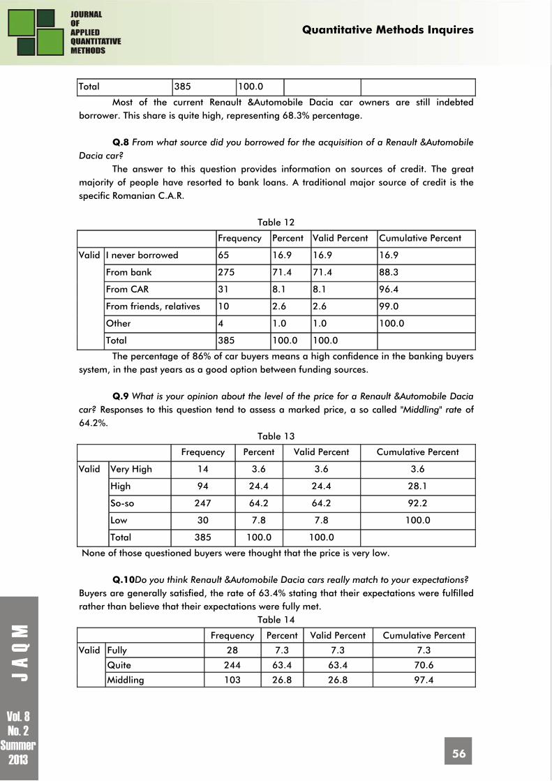
Quantitative Methods Inquires
56
Total 385 100.0
Most of the current Renault &Automobile Dacia car owners are still indebted borrower. This share is quite high, representing 68.3% percentage. Q.8 From what source did you borrowed for the acquisition of a Renault &Automobile Dacia car? The answer to this question provides information on sources of credit. The great majority of people have resorted to bank loans. A traditional major source of credit is the specific Romanian C.A.R.
Table 12
Frequency Percent Valid Percent Cumulative Percent
Valid
I never borrowed 65 16.9 16.9 16.9
From bank 275 71.4 71.4 88.3
From CAR 31 8.1 8.1 96.4
From friends, relatives 10 2.6 2.6 99.0
Other 4 1.0 1.0 100.0
Total 385 100.0 100.0
The percentage of 86% of car buyers means a high confidence in the banking buyers system, in the past years as a good option between funding sources. Q.9 What is your opinion about the level of the price for a Renault &Automobile Dacia car? Responses to this question tend to assess a marked price, a so called "Middling" rate of 64.2%.
Table 13
Frequency Percent Valid Percent Cumulative Percent
Valid
Very High 14 3.6 3.6 3.6
High 94 24.4 24.4 28.1
So-so 247 64.2 64.2 92.2
Low 30 7.8 7.8 100.0
Total 385 100.0 100.0
None of those questioned buyers were thought that the price is very low. Q.10Do you think Renault &Automobile Dacia cars really match to your expectations? Buyers are generally satisfied, the rate of 63.4% stating that their expectations were fulfilled rather than believe that their expectations were fully met.
Table 14
Frequency Percent Valid Percent Cumulative Percent
Valid
Fully 28 7.3 7.3 7.3
Quite 244 63.4 63.4 70.6
Middling 103 26.8 26.8 97.4

Quantitative Methods Inquires
57
Somehow less 10 2.6 2.6 100.0
Total 385 100.0 100.0 In a neutral position there is a percentage of 26.8% of the respondents. Among those who say very little disappointed in what is expected only 2.6% were delivered. Q.11 I believe that possession of Renault &Automobile Dacia car gives…? To this detailed question the most of the respondents have considered possession as a necessity (60.3%).
Table 15
Frequency Percent Valid Percent Cumulative Percent
Valid
gives a certain social status 16 4.2 4.2 4.2
allows a fast and safe travels 135 35.1 35.1 39.2
entails significant costs 2 0.5 0.5 39.7
is a necessity 232 60.3 60.3 100.0
Total 385 100.0 100.0
A proportion of 16% of Renault &Automobile Dacia owners are proud to see that their possession gives a certain social status. An insignificant minority believes that possession incurred the extra expenses. Q.12 If you acquire one of the versions below, please make an order, marking one box depending on your preference ranked no. 1 on the one that best matches your preferences. After data processing the head buyer preferences is Logan, and within easy reach are the new model Stepway and Sandero.
Table 16
Logan Stepway Sandero Logan MCV Pick-up Logan Van
2.57 2.77 2.93 3.1 4.79 4.83
Q.20 Do you think Renault &Automobile Dacia cars are more adequate to Romanian roads? In this issue Renault &Automobile Dacia car owners agreed represent a rate of 66.2% (total agreement means a high proportion of 22.1%, also).
Table 17
Frequency Percent Valid Percent Cumulative Percent
Valid
Total agreement 85 22.1 22.1 22.1
Agreed 255 66.2 66.2 88.3
No-no 41 10.6 10.6 99.0
Disagreement 2 5 5 99.5
Totally disagree 2 5 5 100.0
Total 385 100.0 100.0
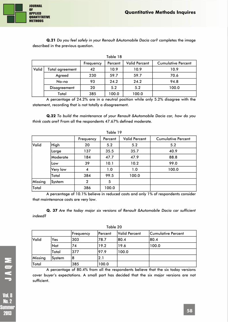
Quantitative Methods Inquires
58
Q.21 Do you feel safely in your Renault &Automobile Dacia car? completes the image described in the previous question.
Table 18
Frequency Percent Valid Percent Cumulative Percent
Valid
Total agreement 42 10.9 10.9 10.9
Agreed 230 59.7 59.7 70.6
No-no 93 24.2 24.2 94.8
Disagreement 20 5.2 5.2 100.0
Total 385 100.0 100.0 A percentage of 24.2% are in a neutral position while only 5.2% disagree with the statement, recording that is not totally a disagreement. Q.22 To build the maintenance of your Renault &Automobile Dacia car, how do you think costs are? From all the respondents 47.67% defined moderate.
Table 19
Frequency Percent Valid Percent Cumulative Percent
Valid
High 20 5.2 5.2 5.2
Large 137 35.5 35.7 40.9
Moderate 184 47.7 47.9 88.8
Low 39 10.1 10.2 99.0
Very low 4 1.0 1.0 100.0
Total 384 99.5 100.0
Missing System 2 5
Total 386 100.0
A percentage of 10.1% believe in reduced costs and only 1% of respondents consider that maintenance costs are very low. Q. 37 Are the today major six versions of Renault &Automobile Dacia car sufficient indeed?
Table 20
Frequency Percent Valid Percent Cumulative Percent
Valid
Yes 303 78.7 80.4 80.4
Not 74 19.2 19.6 100.0
Total 377 97.9 100.0
Missing System 8 2.1
Total 385 100.0 A percentage of 80.4% from all the respondents believe that the six today versions cover buyer’s expectations. A small part has decided that the six major versions are not sufficient.

Quantitative Methods Inquires
59
Q.39 What the general note for Renault &Automobile Dacia car would be, in your opinion?
Table 21
Frequency Percent Valid Percent Cumulative Percent
Valid
5 7 1.8 1.8 1.8
6 20 5.2 5.2 7.0
7 71 18.4 18.4 25.5
8 142 36.9 36.9 62.3
9 135 35.1 35.1 97.4
10 10 2.6 2.6 100.0
Total 385 100.0 100.0
The dominant evaluation is 8 but 9 has a high proportion, too (35.1%). Q.43. Would you recommend someone to buy a Renault &Automobile Dacia car? A very great majority of respondents were favourable to Renault & Automobile Dacia car (a rate of 91.7% and only 8.3% did not recommend buying such a car).
Table 22
Frequency Percent Valid Percent Cumulative Percent
Valid
Yes 353 91.7 91.7 91.7
Not 32 8.3 8.3 100.0
Total 385 100.0 100.0
Q.46 Your occupation is? All the occupations were grouped into 11 representative categories.
10987654
150
100
50
0
Frequency
Mean =8,06
Std. Dev. =1,005
N =385
Figure 1. The Evaluations’ Histogram
Evaluation

Quantitative Methods Inquires
60
The buyers of Renault &Automobile Dacia cars include various occupations, but specialist and employer & managers are the majority of this population.
Table 23
Frequency Percent Valid Percent
Cumulative Percent
Valid
Student 9 2.3 2.3 2.3
Worker 31 8.1 8.1 10.4
Technician / mentor / teacher /clerk
65 16.9 16.9 27.3
Military framework / cop / guard 27 7.0 7.0 34.3
Employer / manager 94 24.4 24.4 58.7
Environmental health professional 10 2.6 2.6 61.3
Specialist / frame with superior training
100 26.0 26.0 87.3
Unemployed 7 1.8 1.8 89.1
Home 2 5 5 89.6
Pensioner 10 2.6 2.6 92.2
Other occupations 30 7.8 7.8 100.0
Total 385 100.0 100.0
Specialists and professionals with higher education called specialists/frame with superior training include all persons who have completed at least one higher education institution but do not occupy management positions.
7. SOME BIVARIATE STATISTICS – ANALYSES All so called bivariate statistics or bivariational data analyses consist in studying and testing hypotheses in the research, in order to investigate the relationship between two variables simultaneously. The papers’ authors researched and underline the link between variational intensity using specific statistical tests. Some interesting connections between variables have been also investigated to explain market phenomena in a so called dependent change with other variable as independent ones (using crosstab and contingency tables for that purpose). Q.40 Some of the components necessary to manufacture the Logan car plants in other states are produced at Automobile Dacia and exported to these destinations. Do you think this brings a Renault &Automobile Dacia brand reputation? and Q. 46 What is you last school’s level of graduation?

Quantitative Methods Inquires
61
Table 24 The Occupation and Prestige Crosstab
Prestige Total Total
agreement Agreed No-
no Disagree-
ment Totally
disagree
Occ
upat
ion
Student 0 9 0 0 0 9
Worker 7 20 4 0 0 31
Technician/mentor/learning or manufacturer/clerk
5 55 5 0 0 65
Military framework/cop/ guard 8 17 2 0 0 27
Employer/manager 50 32 12 0 0 94
Environmental health professional 6 4 0 0 0 10
Specialist/frame with superior training
40 46 11 1 2 100
Unemployed 1 3 3 0 0 7
Home 2 0 0 0 0 2
Pensioner 3 5 2 0 0 10
Other occupations 6 20 3 1 0 30
Total 128 211 42 2 2 385 The respondents, who have been interviewed, thought that the analysed facts make a prestige brand Renault &Automobile Dacia. There are four people who disagree or are in a total disagreement with that idea. A total of 42 respondents can not pronounce about. The agreement means 211 persons or 54.8% of total agreement and 128 persons or 33.2%. Those who believe in the most prestige brand that Renault &Automobile Dacia has won are the managers and owners. Household of two people, who answered this question, both totally agree that the company has gained prestige. Also groups of specialists/professionals with higher education are clearly in favour of the claim. The agreement is 46% complete agreement is 40%. All 9 students have concurred that Dacia will increase prestige. Q. 39 What the general evaluation (note) for Renault &Automobile Dacia car would be, in your opinion? and Q. 49 What your age is, in the next groups or classifications by age?
Table 25 The Age’s Group and the General Evaluation (Note) Crosstab
General evaluation (note) Total 5 6 7 8 9 10
Gro
up o
f ag
e
between 18-29 years 2 5 12 37 12 0 68
between 30-39 years 2 2 11 31 35 3 84
between 40-49 years 3 8 33 42 58 5 149
between 50-59 years 0 5 14 23 27 2 71
60 years and over 0 0 1 9 3 0 13
Total 7 20 71 142 135 10 385

Quantitative Methods Inquires
62
The respondents, giving minimum evaluations or notes, are from the first three age groups (7 persons in these categories). Average score, the lower t also belong to the people aged 18-29 years, an age group that is more favourable assessments from the group of persons aged 30-39 years. This group, during the analysed period marks the highest evaluation, averaging 8.23. Besides the 10 people who gave the maximum score to Renault & Automobile Dacia car are in the groups aged beyond 30 years old, but not over 60.
8. THE NECESSITY OF STATISTICAL TESTS In our marketing research to formulate the conclusions we assume some hypotheses and statistical tests. The hypothesis testing is to identify the one from two hypotheses is correct. The assumptions are made null and alternative hypotheses. We can analyse, for instance, findings Renault & Automobile Dacia (or a Stepway, etc.) car comparative to a car like the Renault brand. The connection between of Renault & Automobile Dacia car’s buyer opinion to a qualitative resemblance like the Renault brand can be put in two hypotheses: 1.Null hypothesis H0: mean subjective assessment Renault & Automobile Dacia (or a Stepway, etc.) car owners is 3 points on a scale of 1 to 5; H0: Μ0 = 3 points 2.Alternative hypothesis: H1: Media subjective assessment is Renault & Automobile Dacia (or a Stepway, etc.) car owners other than 3 points on a scale of 1 to 5 H1: Μ0 ≠ 3 points
Table 26
One-Sample Statistics
N Mean Std. Deviation
Std. Mean error
1.Compared to similar self Sele from the Dacia Renault brand?
385 3.12 0.747 0.038
2.Ordering Stepway 385 3.03 1823 0.093
Table 27
One-Sample Test
Test Value = 3
t df Sig. (2-tailed)
Mean Difference
95% Confidence Interval of the Difference
Lower Upper
1.Against Sele from the car like Renault's Dacia brand?
3277 384 0.001 0.125 0. 05 20
2.Ordering Stepway 0.307 384 0.759 0.029 - 15 21
1. To test this hypothesis Student t test was applied. The t valueobs is 3.277, compared with t0.05, 96 = 1.98 (value for a bilateral test) that tobs > t0.05, 384 and reject H0 accepting the alternative hypothesis. Value significance level (Sig 2-tailed = 0.001) is less than α = 0.05, that rejecting H0. That decision can be taken and the observation of the confidence interval limits, they do not contain the value 0, this means rejecting the

Quantitative Methods Inquires
63
hypothesis H0 and supports the hypothesis H1 that average assessments of Renault & Automobile Dacia car’s buyer believes that the performance of a vehicle Dacia is worse than a car like Renault and varies from 3 points on a scale of 1 to 5. 2. To test this hypothesis Student t test was applied. The t valueobs is 0.307 compared with t0.05, 384 = 1.98 (value for a bilateral test) that tobs < t0.05, 384 null hypothesis and accept H0, rejecting alternative. Value significance level (Sig 2-tailed = 0.759) is larger than α = 0.05, it follows that H0 admits. That decision can be taken and the observation interval confidence limits, it contains the value 0, it means that you accept the hypothesis H0 and reject the alternative hypothesis H1 that average assessments of Renault & Automobile Dacia car’s buyer for Dacia Stepway is 3 points on a scale of 1 to 6. The statistical tests can be used for testing percentages, or average percentage differences, also.
9. SOME CONCLUSIONS OF A QUANTITATIVE MARKETING RESEARCH Largest share among the respondents represented men. The first impulse would be that they are more interested in cars than women, but tests show that the cars are better acquainted in their possession. Although it is noted as a trust declared, Renault & Automobile Dacia car, in excess of 84% scores and is slightly above the 8. Men are more uniform assessments compared to women however the overall rating given by women is higher than that of men with only 0.5%.Variant the most appreciated Logan followed a short distance from the new model on Locle Stepway of three centuries, to the Sandero topping preferences. Sandero lead preferences among women. Regarding the safety of the car Renault & Automobile Dacia gone almost 69% of owners surveyed agree with this statement: I agree 10.9%. I disagree with the statement that 5.2% of subjects generally gives confidence the security offered. Maintenance costs are considered moderate by 47.9% and 35.5% higher, leading to picture to a car with significant maintenance costs. As regards price perception parts are considered rather than 50.5% of subjects with this opinion. Versions are produced in sufficient proportion of 78.8% respondents’ opinion. There is a fairly high confidence in Renault & Automobile Dacia when considered that the Dacia factory and exporting auto parts for other Renault factories. Although respondents do not know about cars made in other Renault sites they believe that this brings a prestigious brand Renault & Automobile Dacia. Respondents believe that the products are known Renault & Automobile Dacia, 80% of respondents answering yes to that question. The Renault & Automobile Dacia cars, through their performance, middle-income class addressed, and the price are the main reasons for its acquisition. To be more attractive it is required several steps like:
the enrichment of variants with sports models, land and small urban movement consumption necessary; improving design and in particular flag over the hood; diversification of optional equipment such as steering controls for audio equipment, EBS braking system, equipped with air conditioning climatronic, and burglar alarm system with remote operated from home, setting the front seats on both horizontal and height of the heating system seats, side airbags, parking sensors, automatic switching of lights at dusk and automatically start the wipers when rain start and adapt their speed to the amount of precipitation fallen; (the customers want to limit the running speed automatic when it is

Quantitative Methods Inquires
64
desired by the driver, and to have the real possibility of adjustment wheel which is now fixed). increasing shelf from 3 years to 4 years or even 5 years after some opinions. Some subjects would guarantee up to 300,000 miles. organizing test drive periodically to improve public approach and the knowledge of Renault & Automobile Dacia car; organization of an open door for the producer in Mioveni; a good understanding of the manufacturing process and technology used to increase confidence in potential buyers; transparency repair operations both in terms of technology and process costing, and reduced repairs, improving management reorganization and technological flows; developing a credit system to facilitate its manufacturer and purchase a vehicle that would contribute both to increase sales and increase confidence in the products produced; flexible manufacturing process to produce copies of personalization to customers desire; self organizing travelling exhibitions in various cities of the country and driving tests for promotion of Renault & Automobile Dacia cars.
10. SOME FINAL REMARKS Renault & Automobile Dacia is undoubtedly on track and may take other measures which can help company to increase its prestige. For a large company it can be even used the Renault & Automobile Dacia employees who may be involved in promotional activities to mark one man. From previous analysis it has been separated the appearance that most buyers have been holding a derivative version of the Dacia Renault 12 and may insist on customer loyalty by providing bonuses for those who are differentiated from the second purchase. Because most of the Renault & Automobile Dacia car’s buyers turned to other sources of credit is necessary to facilitate access to other funding sources available why not some of Renault & Automobile Dacia. That the models currently manufactured are exported to countries from Mioveni with a long tradition in the automotive industry will further increase local confidence in potential buyers that can be explored. Renault & Automobile Dacia brand perception is still largely subjective considered by some buyers that is less than one imported brand in particular German. However Renault & Automobile Dacia cars have entered on the German market without feelings of incisor or inferiority. The same thing happened and the markets of France and Italy, especially in markets where it took place the fleet renewal program…
BIBLIOGRAPHY 1. Balaure, V. Marketing. Bucureşti: Editura Uranus, 2002. 2. Evrard, Y., Pras, B., and Roux, E. Market. Etudes et recherches en marketing. 152-164.
Paris : Ed. Nathan, 1993. 3. Moser, A. Metode de ancheta in investigarea fenomenelor sociale. Bucureşti: Ed.
Ştiinţifică, 1967. 4. Pistol, G., Marketing. Piteşti: Ed.Independenţa Economică. 2001. 5. Săvoiu, G. Cercetări şi modelări de marketing. Bucureşti: Ed. Universitară. 2005
1(Co)Author of the books: Exploratory Domains of Econophysics. News EDEN I &II (2009), Statistica - Un mod stiintific de gandire (2007), Populatia lumii intre explozie si implozie demografica (2006), Cercetari si modelari de marketing. Metode cantitative in cercetarea pietei(2005), Universul preturilor si indicii interpret (2001).