arX

iv:1

911.

0714

5v5

[m

ath.

DG

] 1

4 Se

p 20

21

Geometric calculus on pseudo-Riemannian manifolds

Joseph C. Schindler

SCIPP and Department of Physics, University of California Santa Cruz, Santa Cruz, CA, USA

Email: jcschind@ucsc.edu

September 2020

Abstract

This article provides a pedagogically oriented introduction to geometric (Clifford) calculuson pseudo-Riemannian manifolds. Unlike usual approaches to the topic, which rely on embed-ding the geometric algebra either within a tensor algebra or within a vector manifold frame-work, here we define geometric calculus directly, by elementary methods. In particular we usean axiomatic approach that directly parallels textbook introductions to general relativity andpseudo-Riemannian geometry, so that no structure outside the metrical Clifford bundle of themanifold need be introduced. On this basis we develop the full theory of differential calculus forvector, multivector, and tensor fields.

Mathematics Subject Classification: 15A66, 53B05, 53B21, 53B30, 58A10.

Keywords: Riemannian geometry, smooth manifolds, geometric calculus, multivector fields, dif-ferential geometry, geometric algebra, Clifford algebra, differential forms.

Contents

1 Introduction 22 Survey and motivation 33 Notation and conventions 54 Geometric tangent space 65 Basis frames 76 Scalar and vector fields 87 Multivector fields and the multivector directional derivative 118 Torsion-free multivector directional derivative 159 Tensors 1610 Tensor fields 1911 Gradient, divergence, curl 2212 Differential forms, exterior derivative 2413 Concluding remarks 26A Geometric algebra review 27B Smooth tangent structure 29C Proof of Theorem 11 (MDD preserves grade) 29D Proof of Theorem 14 (MDDs ↔ metric-compatible connections) 30E Gradient and linear transformations 32

1

1 Introduction

Methods of geometric (Clifford) algebra have useful applications throughout physics and mathemat-ics [1–4]. Applying these methods to extend traditional vector and tensor calculus is the domain ofgeometric calculus. Like tensor calculus, it is natural to study geometric calculus in the context ofpseudo-Riemannian manifolds (that is, smooth manifolds with a nondegenerate metric of arbitrarysignature).

Typically geometric calculus is applied to this problem using one of two approaches. One, thealgebraic approach, is typified by textbooks such as [5–7], where a Clifford bundle is defined as aquotient of the tensor bundle of the manifold. The other, the vector manifold approach, is typifiedby textbooks such as [8, 9], where the manifold is itself taken to be embedded within a geometricalgebra. In either case, some additional structure beyond the manifold and its Clifford bundle mustbe used to define the formalism.

Here we will take a slightly different approach where no additional structure is necessary, inorder to more closely parallel standard textbook treatments of pseudo-Riemannian geometry andgeneral relativity. The approach is based on a minimal set of axioms for a multivector directionalderivative (MDD) operator (that is, an extension of the affine connection to act on multivectorfields), encapsulated in Definition 8. The entirety of the framework is derived from these axioms,just as standard Riemannian geometry is based on the axioms for an affine connection [10, 11].

Within this approach, an important point is that it is not trivial to show that the MDD axiomsare self-consistent—that is, it is not obvious that any operator satisfying those axioms exists.Therefore, the direct constructive proof of Theorem 13 (existence) is a key result underpinning theformalism. Once this existence is established, many any other useful properties can be proved fromthe axioms, including that MDDs are grade-preserving, follow product rules for the geometric, dot,and wedge products, and can be used to define the tensor covariant derivative, differential formsexterior derivative, and multivector gradient.

This framework has some useful features. It naturally incorporates arbitrary bases (which maybe holonomic, orthonormal, or neither), metrics of arbitrary signature, and connections both withand without torsion. MDDs will be seen to have powerful properties, and the tensor derivative willbe derived from MDDs based on a chain rule for linear functions. Then straightforward generaliza-tions of the vector calculus gradient, divergence, and curl are introduced, and it is shown that thetheory of differential forms is subsumed.

An important aspect to notice about the geometric algebra approach is that it works onlyin terms of tangent vectors and tangent multivectors, but dual vectors (i.e. covectors) will neverbe introduced. Given a vector basis ei, rather than defining a dual basis in the dual space, oneintroduces a “reciprocal” basis ei (obeying ei ·ej = δij) of vectors in the same space. This is possiblebecause, given the metric, there is a canonical isomorphism identifying covectors with vectors. Thissimplifies certain parts of the theory, but also means these methods can be used only when a metricis present. Nonetheless, it is possible to analyze smooth manifolds by assuming an arbitrary metricand forming only metric-independent results within the framework.

The structure of the paper is as follows.Geometric algebra (the algebra of “multivectors”) is reviewed in Appendix A, while Section 2

provides a brief survey of the framework that will be found in the main text, as well as some furthermotivation for the framework.

Sections 3–6 establish conventions, define a geometric tangent space to the manifold, and reviewthe familiar theories of scalar fields, tangent vector fields, affine connection, and Lie bracket. Thepurpose of this review is both pedagogical, and to provide conventions for the later sections. In theinterest of a self-contained treatment, detailed proofs are given even in the review.

2

The main results occur in Sections 7–10, where we establish the differential theories of multivec-tors, tensors, and differential forms, all in terms of the MDD axioms. Various details and severallonger proofs appear in the appendix.

2 Survey and motivation

Geometric algebra (the algebra of “multivectors”) is reviewed in Appendix A.The following is a summary of the basic formalism to be established for geometric calculus on

pseudo-Riemannian manifolds:

• Let ei be an arbitrary set of basis vector fields (i.e. an arbitrary frame). There exists areciprocal frame ei defined by ei · ej = δij . Metric coefficients and Lie bracket coefficients inthe basis are defined by

ei · ej = gij , [ei, ej ] = Lijk ek ,

and connection coefficients in the basis are defined by

Deiej = Γijk ek

for an affine connection D.

• There are three important types of special basis: orthonormal, holonomic, and gradient. Anorthonormal basis is one such that gij = η(i) δij with η(i) = ±1. A holonomic basis is onesuch that Lijk = 0. A gradient basis is one such that ei = ∇ϕi (gradient ∇ defined later) forsome set ϕi of scalar fields. An orthonormal basis is reciprocal to an orthonormal basis. Aholonomic basis is reciprocal to a gradient basis, and vice-versa.

• We use a special notation for coordinate bases. For a coordinate system xi, coordinate basesare denoted e(xi) (this would usually be denoted ∂

∂xi ), and are holonomic. Coordinate deriva-

tives of a scalar field are then written ∂e(xi)ϕ = ∂ϕ∂xi . The reciprocal basis to e(xi) is the

coordinate gradient basis dxi = ∇xi = gije(xi) obtained from the gradient of the scalarcoordinate functions. These are both vector bases, no dual space was introduced.

• In an arbitrary basis ei (which might be holonomic, orthonormal, or neither), metric-compatibilityand torsion-freeness of the connection are expressed by

Γijk + Γikj = ∂eigjk, Γijk − Γjik = Lijk.

Thus if general connection coefficients are written as

Γijk = 12

(∂eigjk − ∂ekgij + ∂ejgki

)+ 1

2 (Lijk − Ljki + Lkij) + χijk

it immediately follows that the Levi-Civita connection is given by χijk = 0. In general theχijk are called “contorsion coefficients”.

• The affine connection is extended to a “multivector directional derivative” (MDD) by de-manding the product rule

Da(AB) = (DaA)B +A (DaB)

hold on all multivectors A,B. MDDs will be defined axiomatically, and their existence provedby construction. It is also proved from the axioms that MDDs are grade-preserving, and thata similar product rule also holds for the dot and wedge products.

3

• MDDs are extended to act on tensor fields by a direct chain-rule computation. For exampleif T (A,B) is a multilinear function (tensor) with multivector inputs A,B then, by the chainrule, its tensor derivative DaT is defined by

DaT (A,B) = Da(T (A,B)) − T (DaA,B)− T (A,DaB)

where a is a vector and derivatives on the right hand side are MDDs. The relation of thisexpression to the chain rule is clarified in the text. In terms of tensor coefficients, this becomesthe usual

DiTjk = ∂iT

jk + (Γilm gmj)T lk + (Γilm gmk)T jl .

This chain rule definition of DaT is equivalent to the usual covariant derivative definition.

• An MDD operator is not a tensor, since in general Da(ϕA) 6= ϕDa(A) for scalar fields ϕ.However, the difference (D− D) between two MDDs is a tensor. Hence Γijk do not transformlike tensor coefficients, but χijk do.

• In this formalism, one normally thinks of the metric coefficients, rather than the metric tensor.But if desired, the metric tensor can be formally defined by g(a, b) = a · b. Then its tensorderivative is Dg = 0 by metric compatibility.

• The gradient operator D associated with an MDD D is defined by

DA = ei DeiA

on a multivector field A and shown to have some useful properties, including that gradient

DA = D ·A+D ∧A

is equal to the divergence (D ·A ≡ ei ·DeiA) plus the curl (D ∧A ≡ ei ∧DeiA). Multivectorfields with zero gradient are the n-dimensional analogue of complex analytic functions.

• The unique torsion-free MDD is defined as ∇ and its gradient operator ∇ = ei∇ei is a specialcase of D above. It is proved that

d = ∇∧

is completely equivalent to the exterior derivative of differential forms. Consequently, ∇∧ isindependent of the metric even though ∇ is metric-compatible. Identifying the exteriorsubalgebra of geometric algebra with the space of forms, the theory of differential formsis totally subsumed.

One motivation for the approach outlined above is that it can help provide intuitive descriptionsof physical systems. For an example, consider three ways to express the Lagrangian density forrelativistic electrodynamics [3]:

Tensor calculus: L = −14 F

µνFµν +AµJµ Fµν = ∇µAν −∇νAµ

Differential forms: L = −12 F ∧ ∗F +A ∧ ∗J F = dA

Geometric calculus: L = −12 F · F +A · J F = ∇ ∧A .

The corresponding equations of motion (Maxwell’s equations) are

4

Tensor calculus: ∇µFµν = Jν ǫαβµν ∇αFµν = 0

Differential forms: ∗ d ∗ F = J dF = 0

Geometric calculus: ∇ · F = J ∇ ∧ F = 0 .

The geometric calculus operations are just what they look like: they generalize the divergence andcurl from vector calculus. The bottom equations are especially useful because they express bothmetric dependent (divergence term) and independent (curl term) concepts concisely, and help clarifyhow these expressions fit into a larger theoretical framework.

The geometric calculus form of these equations simplifies further, to the single expression

∇F = J.

The divergence and curl equations are the vector and trivector parts respectively (see later sections).This is more than a notational change—the operator ∇ can be inverted by an integral formula,allowing a direct calculation of field strength F from the source J . Geometric calculus also usefullyunifies vector, tensor, and spinor calculus. In particular, spinors are a subset of multivectors, andDirac’s equation can be expressed using the same derivative operator ∇ appearing in Maxwell’sequation [12].

Throughout the rest of the article, the formalism surveyed above is developed in detail.

3 Notation and conventions

Various notations will be defined below—we collect and review some important ones here.Except where noted otherwise, our conventions generally align with Lee [10, 11] for smooth and

Riemannian manifolds, and with Macdonald [4, 13, 14] for geometric algebra. Further review ofgeometric algebra conventions is in Appendix A.

Symbols use will generally abide by the following conventions:

Da,D directional derivative and gradient∇a,∇ torsion-free directional derivative and gradientd torsion-free curl (d = ∇∧) i.e. exterior derivative

α, β, ϕ, . . . scalar fieldsa, b, . . . vector fieldsA,B, . . . multivector fieldsT, S, . . . tensor fieldsei, e

j , Ei, Ej , . . . basis vector fields (basis frames)

eJ , eK , EJ , E

K , . . . basis multivector fields (multivector frames)

xi ≡ xi coordinate systeme(xi) coordinate tangent basis (coordinate frame)

A few more notes will also be useful:

• (Derivative subscripts.) The subscript a in Da and ∇a is a vector, not a basis index. Rather,Dei would be the derivative in the ei basis direction. Several types of directional derivativeappear (affine, multivector, tensor), but there is no danger of ambiguity (except as addressedin Definition 26), since all others derive from the multivector directional derivative, and eachis made clear in context.

5

• (Index placement.) The upper and lower indices in basis frames, for example in ei and ej ,refer to a pair of reciprocal bases (that is, two sets of basis vectors mutually chosen suchthat ei · ej = δij). However, upper and lower index placement for coordinates is meaningless,

so xi ≡ xi. The symbols ei and Ei refer to arbitrary basis frames; whether such frames areorthonormal, holonomic, or neither depends on context. Likewise, the symbol gij may referto the metric in any basis, depending on context, and is not reserved for the coordinate basismetric.

• (Summation convention.) We assume the Einstein summation convention, so that repeatedindices are always summed unless it is explicitly stated otherwise (this excludes indices insidea function argument, for example i in η(i), so that η(i)aiδij would be summed but η(i)δijwould not).

• (Global vs. local fields.) Fields (scalar, vector, etc.) on a manifold will generally be assumedto be defined only locally in a neighborhood of some point, unless the field is explicitly saidto be defined globally.

• (Smoothness.) The term smooth implies that at least as many derivatives exist as are neededfor any calculation, but need not imply infinite differentiability. Fields are assumed smoothunless stated otherwise.

4 Geometric tangent space

Let M be a smooth manifold with a nondegenerate bilinear metric of arbitrary signature (i.e. apseudo-Riemannian manifold). The tangent space TpM (constructed in the usual way [10]) can beextended to a geometric tangent space GTpM at each point, using the pseudo-Riemannian metricas the geometric algebra dot product. Elements of GTpM are tangent multivectors, which containtangent vectors in TpM as a subset. MVF (M) denotes the space of smooth multivector fieldson M (either local or global depending on context). The smooth structure of GTpM is discussedin Appendix B.

We adopt some nonstandard notational conventions for tangent vectors and bases, both to re-duce the emphasis usually placed on coordinate systems, and to better incorporate tangent vectorsinto the larger multivector framework. We mainly work in terms of completely arbitrary vectorbases ei (which may be orthonormal, holonomic, or neither) with the notation:

Arbitrary Basis Tangent Vector Directional Derivative

Standard Notation: (uses coordinates) X Xϕ

New Notation: ei a ∂a ϕ

To distinguish coordinate bases then requires a special notation (with coordinates xi):

Coordinate Basis Tangent Vector Directional Derivative

Standard Notation: ∂∂xi X = Xi ∂

∂xi Xϕ = Xi ∂ϕ∂xi

New Notation: e(xi) a = ai e(xi) ∂a ϕ = ai ∂e(xi)ϕ = ai ∂ϕ∂xi

Note that for coordinates (but not basis vectors) index placement is meaningless (xi ≡ xi) and ischosen for notational convenience. The above notation involves the identification

∂e(xi) =∂∂xi

6

so that e(xi) is the tangent vector pointing in the direction of the coordinate partial derivative.More broadly we write

∂aϕ

rather than a(ϕ) for the directional derivative of scalar field ϕ, emphasizing that TpM is the spaceof “directional derivative directions”.

We denote vector (TpM) basis frames by ei (lowercase latin index). From vector basis framescan be constructed multivector (GTpM) basis frames eJ (uppercase latin index), defined by

eJ = ej0 ∧ . . . ∧ ejn

as in Appendix B. Arbitrary vector fields a = aiei and multivector fields A = AJeJ can be definedin terms of a frame. The definition of smoothness for fields and frames is given in Appendix B. Allfields and frames are assumed smooth unless stated otherwise.

5 Basis frames

A basis frame (or simply “basis”, when the fact we are discussing fields is implied, as below) is asufficiently smooth (see Appendix B) set of vector fields that forms a vector basis at each point.

An arbitrary basis ei is characterized by two important quantities, the metric coefficients gijand Lie bracket coefficients Lijk (Lie bracket defined later) defined by

gij = ei · ej , [ei, ej ] = Lijk ek.

The reciprocal basis ei is defined by ei · ej = δij as always (see Appendix A), so that ei = gijejexpresses the reciprocal basis using the matrix inverse of the metric. In terms of the basis andreciprocal basis one can expand an arbitrary vector field a by

a = ai ei = ai ei

where ai = a · ei = gij aj and ai = a · ei = gij aj.

There are three important types of special basis: orthonormal, holonomic, and gradient bases.They are defined as follows:

Arbitrary Orthonormal Holonomic Gradient

Definition: ei gij = η(i) δij Lijk = 0 ei = ∇ϕi

Reciprocal to: ei = gij ej Orthonormal Gradient Holonomic

To clarify the notation above, a basis is a gradient basis if there is a set of scalar fields ϕi such thateach basis field ei is the gradient of one of the ϕ. The gradient operator ∇ will be defined later.For orthonormal bases the function η(i) = ±1 (for each index) determines the metric signature, andoften one writes the orthonormal metric as ηij ≡ η(i) δij . It is shown below that every holonomicbasis is reciprocal to a gradient basis, and vice versa. Moreover, it is easy to verify that thereciprocal to an orthonormal basis is also orthonormal. In particular an orthonormal basis obeysei = η(i) ei = ±ei, so an orthonormal basis in Euclidean signature is self-reciprocal.

Given a coordinate system xi, the coordinate basis e(xi) is holonomic. On the other hand, eachindividual coordinate xi can be treated as a scalar field. The gradient works out to ∇xi = gij e(xj),ensuring that ∇xi forms a basis reciprocal to e(xi). It will be shown later on that for scalar fields∇ϕ = ∇∧ϕ = dϕ, so we typically write the coordinate gradient in the more suggestive notation dxi.Thus the situation for a coordinate system xi can be summarized by

7

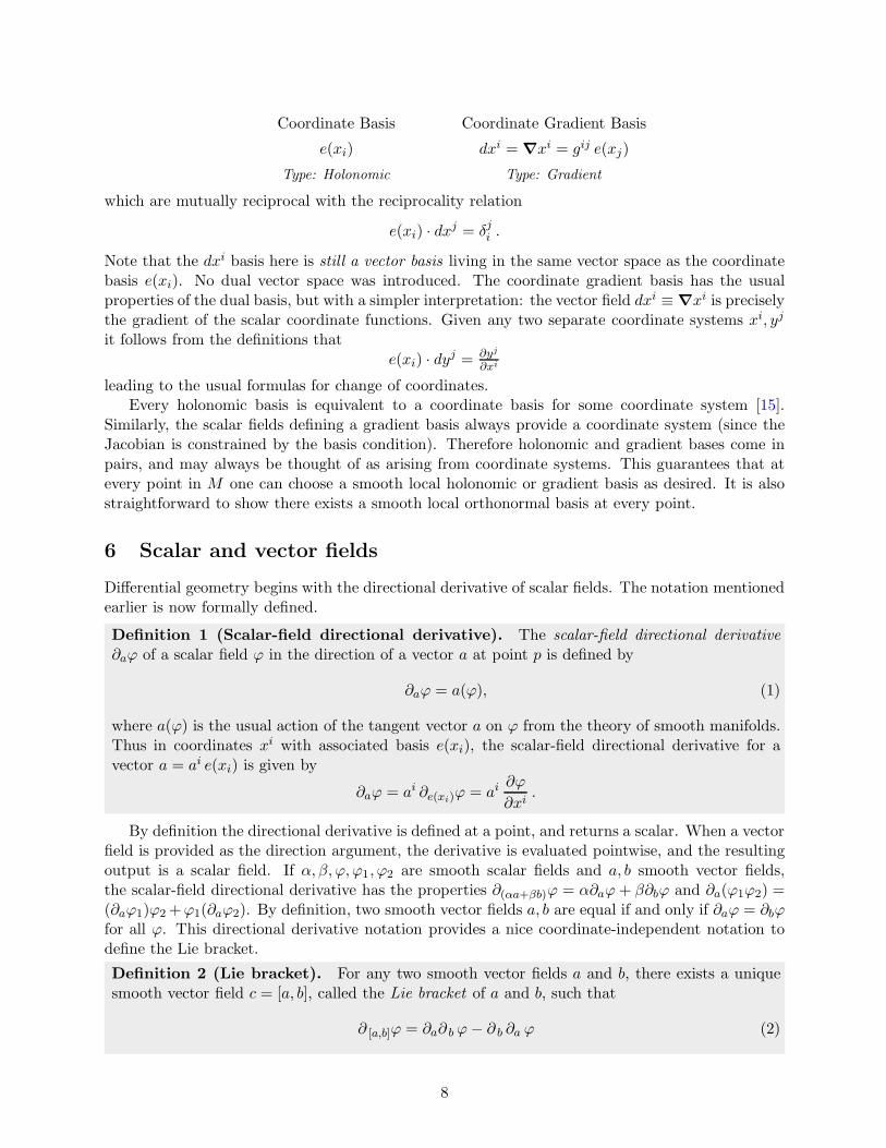
Coordinate Basis Coordinate Gradient Basis

e(xi) dxi = ∇xi = gij e(xj)

Type: Holonomic Type: Gradient

which are mutually reciprocal with the reciprocality relation

e(xi) · dxj = δji .

Note that the dxi basis here is still a vector basis living in the same vector space as the coordinatebasis e(xi). No dual vector space was introduced. The coordinate gradient basis has the usualproperties of the dual basis, but with a simpler interpretation: the vector field dxi ≡∇xi is preciselythe gradient of the scalar coordinate functions. Given any two separate coordinate systems xi, yj

it follows from the definitions thate(xi) · dy

j = ∂yj

∂xi

leading to the usual formulas for change of coordinates.Every holonomic basis is equivalent to a coordinate basis for some coordinate system [15].

Similarly, the scalar fields defining a gradient basis always provide a coordinate system (since theJacobian is constrained by the basis condition). Therefore holonomic and gradient bases come inpairs, and may always be thought of as arising from coordinate systems. This guarantees that atevery point in M one can choose a smooth local holonomic or gradient basis as desired. It is alsostraightforward to show there exists a smooth local orthonormal basis at every point.

6 Scalar and vector fields

Differential geometry begins with the directional derivative of scalar fields. The notation mentionedearlier is now formally defined.

Definition 1 (Scalar-field directional derivative). The scalar-field directional derivative∂aϕ of a scalar field ϕ in the direction of a vector a at point p is defined by

∂aϕ = a(ϕ), (1)

where a(ϕ) is the usual action of the tangent vector a on ϕ from the theory of smooth manifolds.Thus in coordinates xi with associated basis e(xi), the scalar-field directional derivative for avector a = ai e(xi) is given by

∂aϕ = ai ∂e(xi)ϕ = ai∂ϕ

∂xi.

By definition the directional derivative is defined at a point, and returns a scalar. When a vectorfield is provided as the direction argument, the derivative is evaluated pointwise, and the resultingoutput is a scalar field. If α, β, ϕ, ϕ1, ϕ2 are smooth scalar fields and a, b smooth vector fields,the scalar-field directional derivative has the properties ∂(αa+βb)ϕ = α∂aϕ+ β∂bϕ and ∂a(ϕ1ϕ2) =(∂aϕ1)ϕ2+ϕ1(∂aϕ2). By definition, two smooth vector fields a, b are equal if and only if ∂aϕ = ∂bϕfor all ϕ. This directional derivative notation provides a nice coordinate-independent notation todefine the Lie bracket.

Definition 2 (Lie bracket). For any two smooth vector fields a and b, there exists a uniquesmooth vector field c = [a, b], called the Lie bracket of a and b, such that

∂ [a,b]ϕ = ∂a∂ b ϕ− ∂ b ∂a ϕ (2)

8

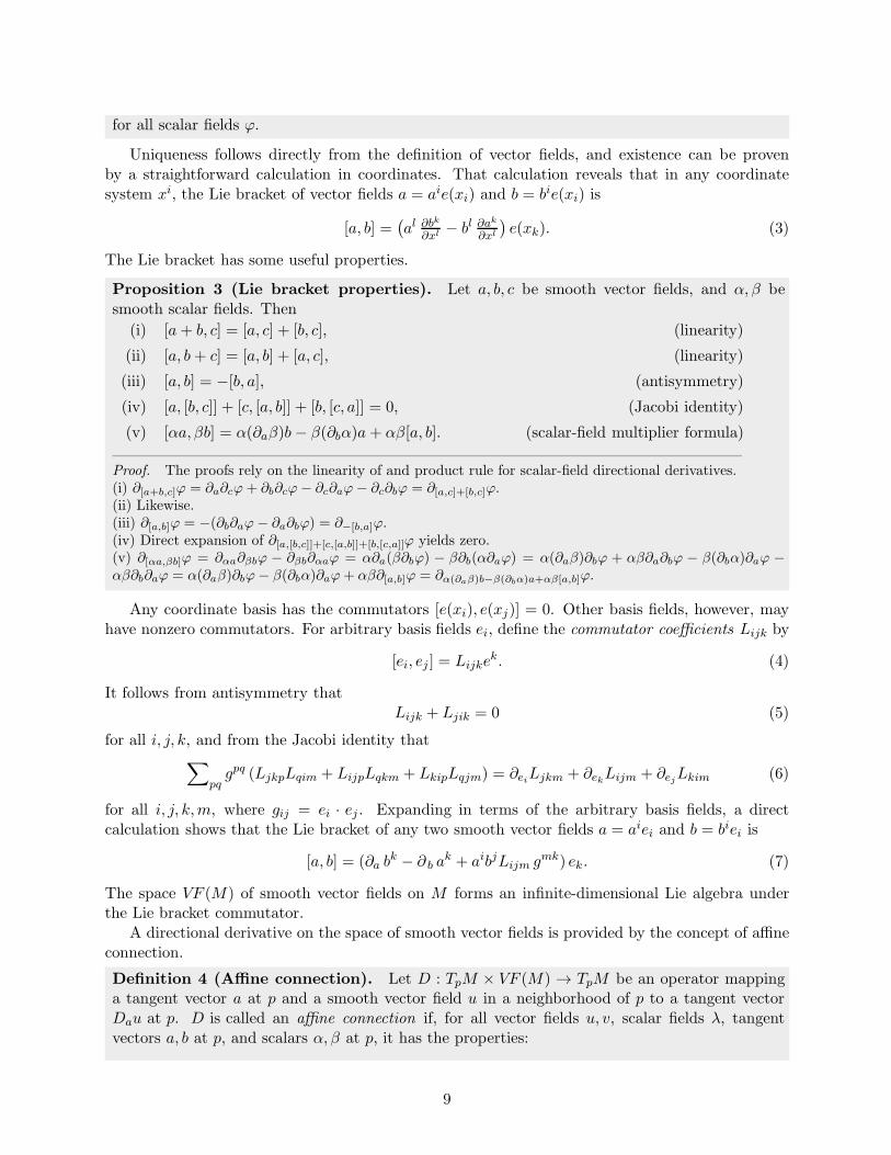
for all scalar fields ϕ.

Uniqueness follows directly from the definition of vector fields, and existence can be provenby a straightforward calculation in coordinates. That calculation reveals that in any coordinatesystem xi, the Lie bracket of vector fields a = aie(xi) and b = bie(xi) is

[a, b] =(al ∂bk

∂xl − bl ∂ak

∂xl

)e(xk). (3)

The Lie bracket has some useful properties.

Proposition 3 (Lie bracket properties). Let a, b, c be smooth vector fields, and α, β besmooth scalar fields. Then

(i) [a+ b, c] = [a, c] + [b, c], (linearity)

(ii) [a, b+ c] = [a, b] + [a, c], (linearity)

(iii) [a, b] = −[b, a], (antisymmetry)

(iv) [a, [b, c]] + [c, [a, b]] + [b, [c, a]] = 0, (Jacobi identity)

(v) [αa, βb] = α(∂aβ)b− β(∂bα)a+ αβ[a, b]. (scalar-field multiplier formula)

Proof. The proofs rely on the linearity of and product rule for scalar-field directional derivatives.(i) ∂[a+b,c]ϕ = ∂a∂cϕ+ ∂b∂cϕ− ∂c∂aϕ− ∂c∂bϕ = ∂[a,c]+[b,c]ϕ.(ii) Likewise.(iii) ∂[a,b]ϕ = −(∂b∂aϕ− ∂a∂bϕ) = ∂−[b,a]ϕ.(iv) Direct expansion of ∂[a,[b,c]]+[c,[a,b]]+[b,[c,a]]ϕ yields zero.(v) ∂[αa,βb]ϕ = ∂αa∂βbϕ − ∂βb∂αaϕ = α∂a(β∂bϕ) − β∂b(α∂aϕ) = α(∂aβ)∂bϕ + αβ∂a∂bϕ − β(∂bα)∂aϕ −αβ∂b∂aϕ = α(∂aβ)∂bϕ− β(∂bα)∂aϕ+ αβ∂[a,b]ϕ = ∂α(∂aβ)b−β(∂bα)a+αβ[a,b]ϕ.

Any coordinate basis has the commutators [e(xi), e(xj)] = 0. Other basis fields, however, mayhave nonzero commutators. For arbitrary basis fields ei, define the commutator coefficients Lijk by

[ei, ej ] = Lijkek. (4)

It follows from antisymmetry thatLijk + Ljik = 0 (5)

for all i, j, k, and from the Jacobi identity that∑

pqgpq (LjkpLqim + LijpLqkm + LkipLqjm) = ∂eiLjkm + ∂ekLijm + ∂ejLkim (6)

for all i, j, k,m, where gij = ei · ej . Expanding in terms of the arbitrary basis fields, a directcalculation shows that the Lie bracket of any two smooth vector fields a = aiei and b = biei is

[a, b] = (∂a bk − ∂ b a

k + aibjLijm gmk) ek. (7)

The space VF (M) of smooth vector fields on M forms an infinite-dimensional Lie algebra underthe Lie bracket commutator.

A directional derivative on the space of smooth vector fields is provided by the concept of affineconnection.

Definition 4 (Affine connection). Let D : TpM × VF (M) → TpM be an operator mappinga tangent vector a at p and a smooth vector field u in a neighborhood of p to a tangent vectorDau at p. D is called an affine connection if, for all vector fields u, v, scalar fields λ, tangentvectors a, b at p, and scalars α, β at p, it has the properties:

9

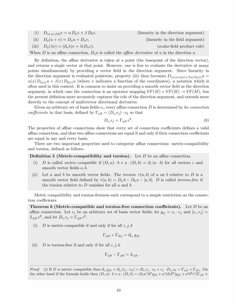
(i) D(α a+β b)v = αDav + β Dbv, (linearity in the direction argument)

(ii) Da(u+ v) = Dau+Dav, (linearity in the field argument)

(iii) Da(λv) = (∂aλ)v + λ(Dav). (scalar-field product rule)

When D is an affine connection, Dau is called the affine derivative of u in the direction a.

By definition, the affine derivative is taken at a point (the basepoint of the direction vector),and returns a single vector at that point. However, one is free to evaluate the derivative at manypoints simultaneously by providing a vector field in the direction argument. Since linearity inthe direction argument is evaluated pointwise, property (iii) then becomes D(α(x) a(x)+β(x) b(x))u =α(x)Da(x)u + β(x)Db(x)u (where x indicates a function of the coordinates), a notation which isoften used in this context. It is common to insist on providing a smooth vector field as the directionargument, in which case the connection is an operator mapping VF (M)× VF (M)→ VF (M), butthe present definiton more accurately captures the role of the direction argument, and extends moredirectly to the concept of multivector directional derivative.

Given an arbitrary set of basis fields ei, every affine connection D is determined by its connectioncoefficients in that basis, defined by Γijk = (Deiej) · ek so that

Deiej = Γijk ek. (8)

The properties of affine connections show that every set of connection coefficients defines a validaffine connection, and that two affine connections are equal if and only if their connection coefficientsare equal in any and every basis.

There are two important properties used to categorize affine connections: metric-compatibilityand torsion, defined as follows.

Definition 5 (Metric-compatibility and torsion). Let D be an affine connection.

(i) D is called metric-compatible if (Dc a) · b + a · (Dc b) = ∂c (a · b) for all vectors c andsmooth vector fields a, b.

(ii) Let a and b be smooth vector fields. The torsion τ(a, b) of a on b relative to D is asmooth vector field defined by τ(a, b) = Da b −Db a − [a, b]. D is called torsion-free ifthe torsion relative to D vanishes for all a and b.

Metric compatibility and torsion-freeness each correspond to a simple restriction on the connec-tion coefficients.

Theorem 6 (Metric-compatible and torsion-free connection coefficients). Let D be anaffine connection. Let ei be an arbitrary set of basis vector fields, let gij = ei · ej and [ei, ej ] =Lijk e

k, and let Deiej = Γijk ek.

(i) D is metric-compatible if and only if for all i, j, k

Γijk + Γikj = ∂ei gjk .

(ii) D is torsion-free if and only if for all i, j, k

Γijk − Γjik = Lijk .

Proof. (i) If D is metric compatible then ∂eigjk = ∂ei(ej · ek) = Deiej · ek + ej ·Deiek = Γijk + Γikj . Onthe other hand if the formula holds then (Dc a) · b+ a · (Dc b) = (∂ca

j)bkgjk + aj(∂cbk)gjk + ajbkci(Γijk +

10

Γikj) = (∂caj)bkgjk + aj(∂cb

k)gjk + ajbk(∂cgjk) = ∂c(ajbkgjk) = ∂c(a · b). (ii) If D is torsion-free then

Deiej − Dejei − [ei, ej ] = (Γijl − Γjil − Lijl)el = 0. Dotting with ek gives the result. Conversely, if the

formula holds then Da b−Db a− [a, b] = aibj(Γijl − Γjil − Lijl)el = 0 using (7).

This leads to a useful standard form for the connection coefficients.

Corollary 7 (Standard form for connection coefficients). Let D be an affine connection.Let ei be an arbitrary set of basis vector fields, let gij = ei · ej and [ei, ej ] = Lijk e

k, and letDeiej = Γijk e

k. Without loss of generality, write

Γijk = 12

(∂eigjk − ∂ekgij + ∂ejgki

)+ 1

2 (Lijk − Ljki + Lkij) + χijk

where χijk are arbitrary coefficients called the contorsion coefficients. Then

(i) D is metric-compatible if and only if χijk + χikj = 0 for all i, j, k.

(ii) D is torsion-free if and only if χijk − χjik = 0 for all i, j, k.

(iii) D is both metric-compatible and torsion-free if and only if χijk = 0 for all i, j, k.

Proof. Let Aijk = 12

(∂eigjk − ∂ekgij + ∂ejgki

). This satisfies Aijk + Aikj = ∂eigjk and Aijk − Ajik = 0.

Next let Bijk = 12 (Lijk − Ljki + Lkij). This satisfies Bijk + Bikj = 0 and Bijk − Bjik = Lijk. (Note

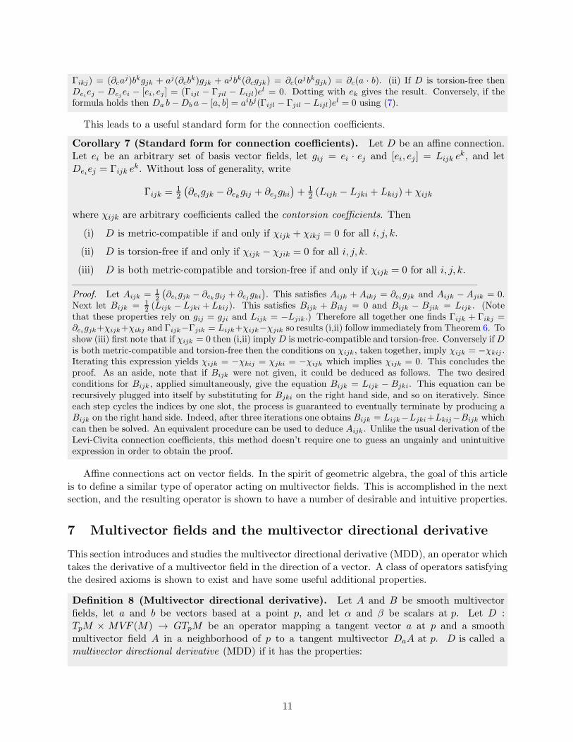
that these properties rely on gij = gji and Lijk = −Ljik.) Therefore all together one finds Γijk + Γikj =∂eigjk+χijk+χikj and Γijk−Γjik = Lijk+χijk−χjik so results (i,ii) follow immediately from Theorem 6. Toshow (iii) first note that if χijk = 0 then (i,ii) implyD is metric-compatible and torsion-free. Conversely ifDis both metric-compatible and torsion-free then the conditions on χijk, taken together, imply χijk = −χkij .Iterating this expression yields χijk = −χkij = χjki = −χijk which implies χijk = 0. This concludes theproof. As an aside, note that if Bijk were not given, it could be deduced as follows. The two desiredconditions for Bijk , applied simultaneously, give the equation Bijk = Lijk − Bjki. This equation can berecursively plugged into itself by substituting for Bjki on the right hand side, and so on iteratively. Sinceeach step cycles the indices by one slot, the process is guaranteed to eventually terminate by producing aBijk on the right hand side. Indeed, after three iterations one obtains Bijk = Lijk−Ljki+Lkij−Bijk whichcan then be solved. An equivalent procedure can be used to deduce Aijk. Unlike the usual derivation of theLevi-Civita connection coefficients, this method doesn’t require one to guess an ungainly and unintuitiveexpression in order to obtain the proof.

Affine connections act on vector fields. In the spirit of geometric algebra, the goal of this articleis to define a similar type of operator acting on multivector fields. This is accomplished in the nextsection, and the resulting operator is shown to have a number of desirable and intuitive properties.

7 Multivector fields and the multivector directional derivative

This section introduces and studies the multivector directional derivative (MDD), an operator whichtakes the derivative of a multivector field in the direction of a vector. A class of operators satisfyingthe desired axioms is shown to exist and have some useful additional properties.

Definition 8 (Multivector directional derivative). Let A and B be smooth multivectorfields, let a and b be vectors based at a point p, and let α and β be scalars at p. Let D :TpM × MVF (M) → GTpM be an operator mapping a tangent vector a at p and a smoothmultivector field A in a neighborhood of p to a tangent multivector DaA at p. D is called amultivector directional derivative (MDD) if it has the properties:

11

(i) D(α a+β b)A = αDaA+ β DbA, (linearity in the direction argument)

(ii) Da〈A〉0 = ∂a〈A〉0 , (scalar-field directional derivative on scalars)

(iii) Da〈A〉1 = 〈Da〈A〉1〉1 , (preserves grade of vectors)

(iv) Da(A+B) = DaA+DaB, (linearity in the field argument)

(v) Da(AB) = (DaA)B +A(DaB). (product rule)

When D is a multivector directional derivative, DaA is called the derivative of the multivectorfield A in the direction a at the point p.

Like the affine connection and scalar-field directional derivative, the MDD is taken at a point,and returns a single multivector at that point, but can be evaluated at many points simultaneouslyby providing a vector field in the direction argument. If one insists on providing a smooth vectorfield in the direction argument, D becomes an operator from VF (M)×MVF (M)→MVF (M).

It is not obvious from the definition whether or not an operator satisfying the above axiomsexists; insisting on the product rule raises the possibility that the definition is self-contradictory oroverconstrained. Fortunately, later we will see that not only does such an operator exist, but manydistinct such operators exist: every metric-compatible connection can be extended to an MDD.Extending non-metric-compatible connections using the above axioms is impossible, however, sincethe resulting operator is self-contradictory and not well-defined.

A few important properties of directional derivatives are derived easily from the definition.

Theorem 9 (MDD properties I). Let D be a multivector directional derivative. Then forevery vector c and all smooth vector fields a and b, the derivative D obeys

(i) Dc (a · b) = (Dc a) · b+ a · (Dc b), (D is metric-compatible.)

(ii) Dc (a ∧ b) = (Dc a) ∧ b+ a ∧ (Dc b). (D is wedge-compatible on vectors.)

Proof. Expand Dc (a · b) = Dc (ab + ba)/2 with the product rule, note that Dc a and Dc b are vectors bydefinition of D, and regroup terms to form the right hand side. Similarly for Dc (a ∧ b) = Dc (ab − ba)/2.

Thus the formalism admits only metric-compatible derivatives. This extra restrictiveness is aresult of unifying the scalar and vector derivatives into a single operator such that scalar-valuedproducts of multivectors have a well-defined derivative.

Another important property which a directional derivative may have is to preserve grade.

Proposition 10 (Grade-preserving). An operator D is called grade-preserving if for everyvector a and smooth multivector field A, it obeys the equivalent conditions

(i) Da〈A〉k = 〈Da〈A〉k〉k for all grades k,

(ii) 〈DaA〉k = Da〈A〉k for all grades k.

Proof. It is claimed that (i) is equivalent to (ii). This is shown as follows.(i→ii) 〈DaA〉k =

∑j〈Da〈A〉j〉k =

∑j〈〈Da〈A〉j〉j〉k =

∑j Da〈A〉j δjk = Da〈A〉k.

(ii→i) 〈Da〈A〉k〉k = 〈〈DaA〉k〉k = 〈DaA〉k = Da〈A〉k.

Interestingly, the product rule is strong enough to ensure that every MDD is grade-preserving.

Theorem 11 (Grade-preserving). The axioms of Definition 8 imply that every multivectordirectional derivative is grade-preserving.

Proof. The proof is obtained by working in an orthonormal basis and observing a simple pattern: when

12

evaluating the directional derivative of strings of orthonormal basis vectors, potentially non-grade-preservingterms come in pairs which together vanish by metric compatibility. Unfortunately there is no simple no-tation to show the proof algebraically, so the full proof is fairly involved. The full proof is given inAppendix C.

This result supports the intuition that a directional derivative represents a limit of differences.It has as a corollary some useful properties.

Corollary 12 (MDD properties II). Let D be a multivector directional derivative. Then forall smooth multivector fields A,B and vectors c, the derivative D obeys

(i) Dc (A · B) = (DcA) · B +A · (DcB), (D is dot-compatible)

(ii) Dc (A ∧B) = (DcA) ∧B +A ∧ (DcB), (D is wedge-compatible)

(iii) If I is a smooth unit pseudoscalar field, Dc I = 0.

Proof. (i) Using linearity, the definition of the inner product, grade-preservation, and the product rule,one finds that Dc(A · B) =

∑jk Dc〈〈A〉j〈B〉k〉k−j =

∑jk (Dc〈A〉j · 〈B〉k + 〈A〉j ·Dc〈B〉k) = (DcA) · B +

A · (DcB). (ii) Likewise. (iii) Let Ei be an orthonormal basis, and suppose without loss of generalitythat DEi

Ej = γijkEk. Metric compatibility with orthonormality implies γijk + γikj = 0. Every smooth

unit pseudoscalar field is equal to I = ±E1 ∧ . . . ∧ En, where n is the dimension of M so all of the Ei

are represented in the product. Consider the first term in the product rule expansion for DEiI, which is

±(±γi1kEk) ∧ . . . ∧ En. Within this term, the k = 1 term vanishes since γijj = 0. Meanwhile the k 6= 1terms vanish by antisymmetry since every Ek for k 6= 1 is already represented in the wedge product. Thusthe first term in the product rule expansion is zero, and all other terms in the expansion vanish for thesame reason. Thus DaI = 0 by linearity in the direction.

Having surveyed some of the properties a multivector directional derivative would have if itexists, it is time to turn to the question of existence. The issue is not trivial, but fortunately theresult works out neatly, as summarized in the following theorems.

Multivector directional derivatives exist.

Theorem 13 (Existence of MDDs). For any metric-compatible affine connection D, thereexists a multivector directional derivative D that equals D when restricted to act only on vectors.

Proof. Proved by construction in Appendix D.

And they are in bijective correspondence with metric-compatible affine connections.

Theorem 14 (MDDs ←→ metric-compatible connections). The restriction to act on vec-tor fields is a bijection from multivector directional derivatives to metric-compatible affine con-nections.

Proof. The axioms of Definition 8 with Theorem 9 ensure that if any D exists the restriction D of D is ametric-compatible affine connection. Expanding in a canonical multivector frame shows that any DA canbe evaluated in terms of D, thus D = D′ implies D = D′ so the map is one-to-one. By Theorem 13, forany metric-compatible affine connection D, there exists an MDD D that restricts to D. Thus MDDs existand the map is onto, so the map is a bijection.

Because of this correspondence, multivector directional derivatives can be uniquely specified bya set of metric-compatible connection coefficients. These can be expressed in terms of an arbitraryvector basis ei such that

gij = ei · ej , [ei, ej ] = Lijk ek ,

13

with reciprocal basis ei such that ei · ej = δij, as usual.

Corollary 15 (Connection coefficients). A multivector directional derivative D is uniquelyspecified by its connection coefficients Γijk in any vector basis ei, defined by

Deiej = Γijk ek,

which can be arbitrary other than the restriction

Γijk + Γikj = ∂ei gjk.

Proof. By Theorem 14, each metric-compatible affine connection extends uniquely to a multivector direc-tional derivative.

Equivalently, the connection coefficients can be parameterized in terms of the contorsion coeffi-cients, separating out the standard term.

Corollary 16 (Contorsion coefficients). A multivector directional derivative D is uniquelyspecified by its contorsion coefficients χijk in any vector basis ei, which can be arbitrary otherthan the restriction

χijk + χikj = 0 .

With Γijk as in Corollary 15, the contorsion coefficients χijk are defined by

Γijk = 12

(∂eigjk − ∂ekgij + ∂ejgki

)+ 1

2 (Lijk − Ljki + Lkij) + χijk .

Additionally, D is torsion-free if and only if χijk ≡ 0.

Proof. Torsion for multivector derivatives is defined in the following section. The rest follows immediatelyfrom Corollaries 15 and 7.

It is also sometimes useful to know the directional derivatives of the reciprocal basis. With thefollowing theorem it becomes easy to evaluate derivatives with any combination of the basis andreciprocal basis elements.

Proposition 17 (Reciprocal connection formula). Let D be an MDD with connectioncoefficients defined by Deiej = Γijk e

k. Then

Deiej = −(Γilm gmj) el

gives a formula for the derivatives of the reciprocal basis.

Proof. Deiej = Dei(g

jmem) = ∂ei(gjm) em + gjmDei(em) = (∂ei (g

jm)gml + gjm Γiml)el = (−∂ei(gml) +

Γiml)gjm el = −Γilmgjm el. The preceding steps made use of metric compatibility in the form ∂eigjk =

Γijk + Γikj and used a product rule expansion of the form ∂ei(gjmgmk) = 0.

This section has established the existence of a set of natural directional derivative operators onthe space of multivector fields. Compared to affine connections, multivector directional derivativeoperators naturally act on a more useful variety of objects, obey a more intuitive product rule, andhave useful properties arising from a minimal set of assumptions.

14

8 Torsion-free multivector directional derivative

We have seen that each multivector directional derivative (MDD) uniquely corresponds to a metric-compatible affine connection. Also like affine connections, MDDs can be characterized by theirtorsion, and there is a unique torsion-free MDD corresponding to the Levi-Civita affine connection.

The definition of torsion for an MDD is the same as for affine connections (see Definition 5).It was already shown that there is a unique metric-compatible torsion-free affine connection. Thisleads immediately to the following statement.

Proposition 18 (Torsion-free MDD). There is a unique torsion-free multivector directionalderivative with contorsion coefficients

χijk = 0

which is given the special notation ∇ and called the torsion-free (or Levi-Civita) derivative.

Proof. Existence is guaranteed by Theorem 14. Uniqueness and χijk = 0 follow from Corollary 7.

It is convenient to also have a special notation for the torsion-free connection coefficients.

Corollary 19 (Torsion-free connection coefficients). The connection coefficients Γijk forthe torsion-free derivative are defined by ∇eiej = Γijk e

k in an arbitrary basis ei, and given by

Γijk = 12

(∂eigjk − ∂ekgij + ∂ejgki

)+ 1

2 (Lijk − Ljki + Lkij) .

These are called the standard (or Levi-Civita) connection coefficients.

Proof. Set χijk = 0 in general form of Γijk (see Corollary 16).

In standard Riemannian geometry, the induced affine connection on an embedded submanifoldof Euclidean Rn is always metric-compatible and torsion-free [11]. Also, geodesics are autoparallelsof the metric-compatible torsion-free connection. These facts motivate the usual acceptance of theLevi-Civita connection as the natural choice of connection on arbitrary manifolds. In the presentcontext, all MDDs are metric-compatible, and we identify the unique torsion-free derivative as anatural choice of MDD. The theory of embedded submanifolds has not been explicitly written downyet in the current context, but presumably the same special properties of the torsion-free derivativecontinue to hold.

Every MDD D can be expressed as the sum of the torsion-free derivative ∇ and a contorsionoperator Q.

Definition 20 (Contorsion operator). Let D be an MDD. Then D can be expressed by

DaA = ∇aA+QaA

Where Q is called the contorsion operator for D.

The contorsion operator has some useful properties.

Proposition 21 (Contorsion operator properties). Let Q = D − ∇ be the contorsionoperator for an MDD D. Then

15

(i) Q has all the properties of Definition 8 except that 8(ii) is replaced by Qaϕ = 0 forscalar fields. Also Q is grade-preserving.

(ii) Qeiej = χijk ek.

(iii) Q is a tensor field (see Section 10).

Proof. (i) All properties follow from direct calculation applying the properties of D and ∇. (ii) Directcalculation. (iii) Q is a tensor field if it is pointwise linear in both arguments. It is automatically pointwiselinear in the direction argument by definition. In the field argument it is pointwise linear since it obeys theproduct rule and annihilates scalar fields: Qa(ϕA) = Qa(ϕ)A + ϕQa(A) = ϕQa(A).

Since the contorsion operator is a tensor field, it can also be called the contorsion tensor. Incontrast, neither D nor ∇ are tensor fields, since they violate pointwise linearity. Thus, under achange of basis, the χijk transform like tensor coefficients while the Γijk do not.

In a holonomic orthonormal basis the torsion-free derivative has Γijk ≡ 0. It follows that amanifold is flat (in the usual sense of having zero Riemann curvature and being locally isometric toa Euclidean or Minkowski space of some signature) if and only if there exists a smooth holonomicorthonormal basis.

9 Tensors

This section generalizes the notion of tensor, from a tensor on a vector space to a tensor on ageometric algebra. The next section will then consider tensor fields on a manifold.

Typically a tensor is defined as a multilinear map from several copies of a vector space (and/orits dual) to R. When a vector space is extended to a geometric algebra, how should the notion oftensor be extended?

There are several ways one could do so. A straightforward approach would be to simply applythe usual definition using the vector subspace of multivectors. This seems not to make enough useof the power of geometric algebra. On the other extreme, one could take a tensor to be a multilinearmap of several copies of the geometric algebra back to itself; this would be a bit too general foreasy analysis, however, and would undermine the concepts of tensor rank and signature. Each ofthese could be said to capture the basic idea that a tensor is a multilinear function of multivectors.

We will use a definition, in the same spirit, which is a middle ground of those extremes; the inputsand output of the multilinear map are each restricted to a fixed-grade subspace of the geometricalgebra. Since the geometric algebra approach has identified vectors with their duals, there will beno need to include the dual space.

Definition 22 (Tensor). Let A be a geometric algebra. Denote by 〈A〉k the linear space ofgrade-k multivectors in A. Then a map

T : 〈A〉k1 × . . . × 〈A〉kN → 〈A〉k0

is called a tensor on A if it is multilinear, meaning that for every input slot

T (. . . , αA+ βB, . . .) = αT (. . . , A, . . .) + β T (. . . , B, . . .)

for all scalars α, β and valid (correct grade for input slot) multivectors A,B.If T is a tensor then its signature is (k1, . . . , kN : k0), its rank is k1 + . . . + kN + k0, and its

number of inputs is N .

16

Traditional tensors have, in this formalism, the signature (1, . . . , 1 : 0). One often finds, however,that the practice of setting k0 = 0 in the traditional definition can require annoying maneuvering tomake multilinear maps into tensors (for example when converting the Riemann curvature functionto the Riemann tensor). Allowing more general tensor outputs is one benefit of the multivectorformalism.

Tensors can be manipulated in various ways. (Note: to simplify notation in the remainder ofthe section, assume input multivectors in tensor arguments always have the correct grade.)

Proposition 23 (Tensor operations). Tensors on a geometric algebra A admit the followingoperations:

(i) Addition.(T + S)(A, . . . , B) = T (A, . . . , B) + S(A, . . . , B) .

(ii) Scalar multiplication.(αT )(A, . . . , B) = αT (A, . . . , B).

(iii) Multiplication. For tensors with scalar outputs (signatures (. . . : 0)):

(T ⊗ S)(A, . . . , B,C, . . . ,D) = T (A, . . . , B)S(C, . . . ,D) .

This is called the tensor product.

(iv) Contraction. A tensor of signature (. . . , 1, . . . , 1, . . . , : k0) (that is, a tensor with at leasttwo grade-1 inputs) can be contracted:

T (. . . , . . . , . . .) =∑

i

T (. . . , ei, . . . , ei, . . .) ,

where ei is an arbitrary basis. The contraction is well-defined, since it can be shown to beindependent of the evaluation basis. The result is a tensor of signature (. . . , . . . , . . . , : k0)(two fewer inputs and rank reduced by 2).

Proof. (i-iii) Trivial. (iv) T is independent of the evaluation basis. Let ei and Ei be any two bases.Suppressing unnecessary arguments, we now show that T = T (ei, e

i) = T (Ei, Ei) (with summation con-

vention). The proof is direct: T (ei, ei) = T ((ei · E

j)Ej , (ei · Ek)E

k) = (ei · Ej)(ei · Ek) T (Ej, E

k) =(Ej · Ek) T (Ej, E

k) = δjk T (Ej, Ek) = T (Ej , E

j). The proof also confirms that the order of the upperand lower index are unimportant.

The zero function Z(A, . . . , B) = 0 is a valid tensor (the zero tensor) for any signature (k0 canbe arbitrary since the zero multivector counts as every grade). Given the zero tensor, it can beshown that the space of tensors of a fixed signature forms a finite-dimensional linear space underaddition and scalar multiplication. It is implicit in the above notation that the operations of additionand scalar multiplication each operate within a space of fixed signature, while multiplication andcontraction operate in the space of all tensors of arbitrary signature.

It is sometimes useful to express tensors in terms of components. In general, the components ofan arbitrary tensor relative to the multivector basis eJ (with reciprocal basis eJ ) are defined by

T (eJ1 , . . . , eJN ) = TJ1 ... JNJ0 eJ0 , (9)

where the multivector basis elements are evaluated only at the grade appropriate for each slot.Components for the same tensor can also be evaluated in the reciprocal basis,

T (eJ1 , . . . , eJN ) = T J1 ... JNJ0 eJ0 , (10)

17

which are written with an upper index. Alternately, mixed up-down tensor components can beobtained by choosing to evaluate each slot using the basis or reciprocal basis. Vector basis indices(corresponding to grade-1 slots) can be raised and lowered with the metric, as seen below, butgeneral multivector basis indices cannot.

When higher grade multivectors are involved, the component notation is a little bit clumsy.Each multivector index J is equivalent to a sequence of several vector indices j, so that, written outfully in terms of vector indices, the number of vector indices is equal to the rank of T . But sincenot every sequence of vector basis elements is represented in the multivector basis, the rank alonedoes not uniquely determine the number of independent components of a tensor; this number can,however, be determined from the signature. On the other hand, if all indices are vector basis indices,the total number of independent components is d r, where r is the rank and d is the dimension ofthe space of vectors.

Components are most useful when working with traditional tensors (of signature (1, . . . , 1 : 0)).In that case,

T (ej1 , . . . , ejN ) = Tj1 ... jN , (11)

and likewise for the upper index components in the reciprocal basis, or mixed components usingboth bases. For a vector basis one has ei = gijej so that, by linearity, component indices can beraised or lowered with the metric, for example as in

T ij = T (ei, ej) = T (gikek, ej) = gik T (ek, ej)

= gik Tkj .(12)

Similarly, the basis transformation formula for components is derived by linearity, from

T (ej1 , . . . , ejN ) = T ((ej1 ·Ek1)Ek1 , . . . , (ejN · E

kN )EkN )

= (ej1 · Ek1) . . . (ejN · E

kN ) T (Ek1 , . . . , EkN ) ,(13)

for arbitrary vector bases ei and Ei. Corresponding formulas in terms of upper or mixed componentscan be extrapolated straightforwardly. Moreover, basically the same formalism holds for tensors ofsignature (1, . . . , 1 : 1) — as long as only vector basis indices are involved, indices behave the sameas in traditional treatments.

Every vector can be naturally identified with a certain tensor, which we call its tensor conjugate.For any vector b, define the tensor b acting on a vector input a by

b (a) = b · a . (14)

This b tensor is the object usually called the one-form conjugate to the vector b. In the case ofreciprocal basis frames, their properties ensure that as tensors they obey

ei (ej) = ei · ej = δij , (15)

a property which will be useful below.More generally, we can provide a tensor conjugate to any fixed-grade multivector. Let Bk be a

multivector of grade k. The tensor Bk conjugate to Bk is a tensor mapping k vector inputs to ascalar (signature (1, . . . , 1 : 0) with k input slots), defined by

Bk (a1, . . . , ak) = Bk · (a1 ∧ . . . ∧ ak) . (16)

This is the usual tensor representation of a k-form. There is also an alternate way to map grade-kmultivectors to tensors, defined by

Bk (A) = Bk · 〈A〉k , (17)

18

resulting in a tensor of signature (k : 0). In both (16) and (17) the grade index would not usuallybe made explicit, but it is given in these cases to clarify how the grade affects the definitions.Clearly, there is a close relationship between the two possibilities, and it seems likely that eachcould prove useful in different situations. Although (17) is more in line with the spirit of themultivector approach, we take (16) as the standard definition in order to make closer contact withstandard tensor calculus.

One can multiply the tensor conjugates a, b of vectors a, b via the tensor product, giving

(a⊗ b) (c, d) = (a · c)(b · d), (18)

with components(a⊗ b) (ei, ej) = (a · ei)(b · ej) = ai bj . (19)

Thus arbitrary tensors of the traditional type (signature (1, . . . , 1 : 0)) be built up in terms of thetensor product as

T = Tj1 ... jN e j1 ⊗ . . .⊗ e jN . (20)

This is a completely general tensor of signature (1, . . . , 1 : 0). Applying the definition of the tensorproduct along with (15) shows that components in (20) are consistent with (11). While this formof tensor notation is sometimes useful, it also tends to obscure the basic nature of a tensor as afunction, and here we avoid it when possible.

This section has defined tensors on a geometric algebra, studied some of their basic properties,and connected the present definitions to traditional ones. Next this is extended to study tensorfields on a manifold.

10 Tensor fields

In traditional differential geometry, and especially in general relativity, tensor fields are given a roleof utmost significance. Even vectors, the most basic objects of the theory, are usually treated as aspecial case of tensors. This leads to a development of tensor calculus in which the role of vectorsas geometric objects and the role of tensors as linear maps are mixed together. As a result, thenatural product rule for multivectors (see above) and natural chain rule for tensors (see below) eachbecome obscured. The geometric algebra approach allows somewhat more conceptual clarity, byseparating the role of multivectors (geometric objects), from the role of tensors (linear maps). Thishelps facilitate a simple derivation of the tensor covariant derivative from the chain rule.

Recall from the previous section that a tensor is defined as a linear operator on a geometricalgebra. In the case of a tensor field on a manifold, the underlying geometric algebra at each pointis the geometric tangent space GTpM . Tensor fields are defined only when the tensor at every pointhas the same signature, as follows. (Note that the definition is rather informal. We avoid a moreformal definition, to avoid introducing the language of bundle sections, as it would not contributemuch to the discussion.)

Definition 24 (Tensor field). A tensor field T of signature S = (k1, . . . , kN : k0) is anassignment of a tensor of signature S on GTpM to each point on (or in a neighborhood on) M .A tensor field is called smooth if smooth inputs always lead to a smooth output.

Each point is assigned its own multilinear function. It follows that the multilinearity propertyof a tensor field is evaluated pointwise, so that even for a non-constant scalar field ϕ, the tensorfield T has the pointwise linearity T (ϕA) = ϕT (A). A map like T which has linearity with respectto constant scalars, but not to non-constant scalar fields, is not a tensor field (the multivector

19

directional derivative Da in the direction of a fixed vector field a, for example, is not a tensor fieldfor precisely this reason).

Tensor fields admit the same operations as tensors (see Proposition 23), with each operationbeing evaluated pointwise. Tensor fields also admit the additional operation of local scalar mul-tiplication (multiplication by a non-constant scalar field); the difference between this and globalscalar multiplication should be clear from context. The space of tensor fields of a fixed signatureforms an infinite-dimensional linear space under addition and global scalar multiplication. Thebasic definitions and operations for tensor fields have now been established.

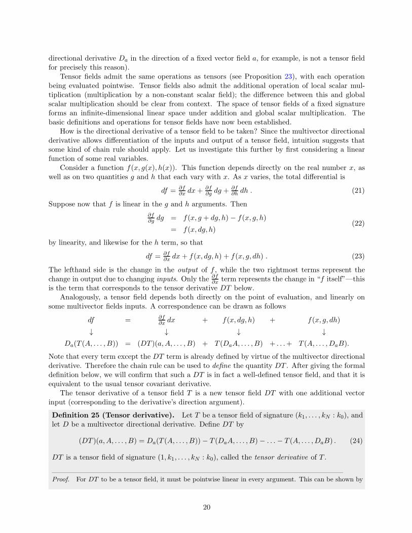
How is the directional derivative of a tensor field to be taken? Since the multivector directionalderivative allows differentiation of the inputs and output of a tensor field, intuition suggests thatsome kind of chain rule should apply. Let us investigate this further by first considering a linearfunction of some real variables.

Consider a function f(x, g(x), h(x)). This function depends directly on the real number x, aswell as on two quantities g and h that each vary with x. As x varies, the total differential is

df = ∂f∂x

dx+ ∂f∂g

dg + ∂f∂h

dh . (21)

Suppose now that f is linear in the g and h arguments. Then

∂f∂g

dg = f(x, g + dg, h) − f(x, g, h)

= f(x, dg, h)(22)

by linearity, and likewise for the h term, so that

df = ∂f∂x

dx+ f(x, dg, h) + f(x, g, dh) . (23)

The lefthand side is the change in the output of f , while the two rightmost terms represent thechange in output due to changing inputs. Only the ∂f

∂xterm represents the change in “f itself”—this

is the term that corresponds to the tensor derivative DT below.Analogously, a tensor field depends both directly on the point of evaluation, and linearly on

some multivector fields inputs. A correspondence can be drawn as follows

df = ∂f∂x

dx + f(x, dg, h) + f(x, g, dh)

↓ ↓ ↓ ↓

Da(T (A, . . . , B)) = (DT )(a,A, . . . , B) + T (DaA, . . . , B) + . . .+ T (A, . . . ,DaB).

Note that every term except the DT term is already defined by virtue of the multivector directionalderivative. Therefore the chain rule can be used to define the quantity DT . After giving the formaldefinition below, we will confirm that such a DT is in fact a well-defined tensor field, and that it isequivalent to the usual tensor covariant derivative.

The tensor derivative of a tensor field T is a new tensor field DT with one additional vectorinput (corresponding to the derivative’s direction argument).

Definition 25 (Tensor derivative). Let T be a tensor field of signature (k1, . . . , kN : k0), andlet D be a multivector directional derivative. Define DT by

(DT )(a,A, . . . , B) = Da(T (A, . . . , B))− T (DaA, . . . , B)− . . .− T (A, . . . ,DaB) . (24)

DT is a tensor field of signature (1, k1, . . . , kN : k0), called the tensor derivative of T .

Proof. For DT to be a tensor field, it must be pointwise linear in every argument. This can be shown by

20

direct calculation using the pointwise linearity of T and the multivector directional derivative properties.The key step is to note that Da(T (αA)) − T (Da(αA)) = αDa(T (A)) − αT (DaA) by cancellation of theunwanted (∂aα)T (A) terms.

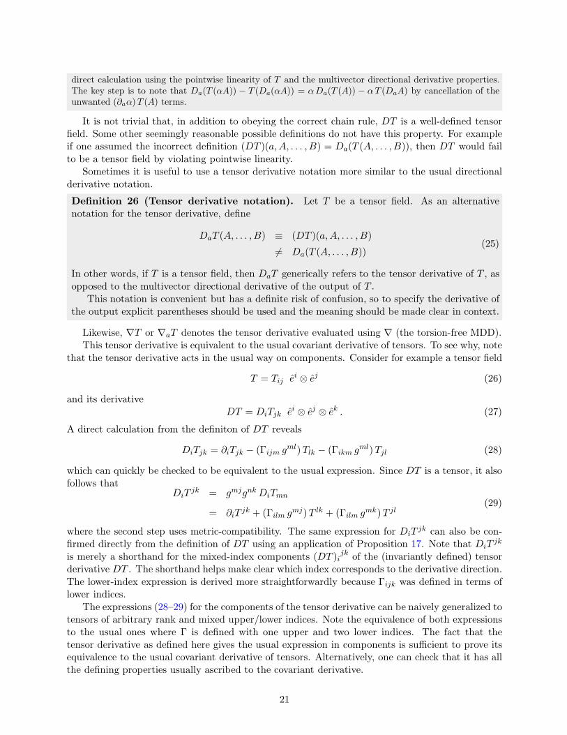
It is not trivial that, in addition to obeying the correct chain rule, DT is a well-defined tensorfield. Some other seemingly reasonable possible definitions do not have this property. For exampleif one assumed the incorrect definition (DT )(a,A, . . . , B) = Da(T (A, . . . , B)), then DT would failto be a tensor field by violating pointwise linearity.

Sometimes it is useful to use a tensor derivative notation more similar to the usual directionalderivative notation.

Definition 26 (Tensor derivative notation). Let T be a tensor field. As an alternativenotation for the tensor derivative, define

DaT (A, . . . , B) ≡ (DT )(a,A, . . . , B)

6= Da(T (A, . . . , B))(25)

In other words, if T is a tensor field, then DaT generically refers to the tensor derivative of T , asopposed to the multivector directional derivative of the output of T .

This notation is convenient but has a definite risk of confusion, so to specify the derivative ofthe output explicit parentheses should be used and the meaning should be made clear in context.

Likewise, ∇T or ∇aT denotes the tensor derivative evaluated using ∇ (the torsion-free MDD).This tensor derivative is equivalent to the usual covariant derivative of tensors. To see why, note

that the tensor derivative acts in the usual way on components. Consider for example a tensor field

T = Tij ei ⊗ ej (26)

and its derivativeDT = DiTjk ei ⊗ ej ⊗ ek . (27)

A direct calculation from the definiton of DT reveals

DiTjk = ∂iTjk − (Γijm gml)Tlk − (Γikm gml)Tjl (28)

which can quickly be checked to be equivalent to the usual expression. Since DT is a tensor, it alsofollows that

DiTjk = gmjgnk DiTmn

= ∂iTjk + (Γilm gmj)T lk + (Γilm gmk)T jl

(29)

where the second step uses metric-compatibility. The same expression for DiTjk can also be con-

firmed directly from the definition of DT using an application of Proposition 17. Note that DiTjk

is merely a shorthand for the mixed-index components (DT )ijk of the (invariantly defined) tensor

derivative DT . The shorthand helps make clear which index corresponds to the derivative direction.The lower-index expression is derived more straightforwardly because Γijk was defined in terms oflower indices.

The expressions (28–29) for the components of the tensor derivative can be naively generalized totensors of arbitrary rank and mixed upper/lower indices. Note the equivalence of both expressionsto the usual ones where Γ is defined with one upper and two lower indices. The fact that thetensor derivative as defined here gives the usual expression in components is sufficient to prove itsequivalence to the usual covariant derivative of tensors. Alternatively, one can check that it has allthe defining properties usually ascribed to the covariant derivative.

21

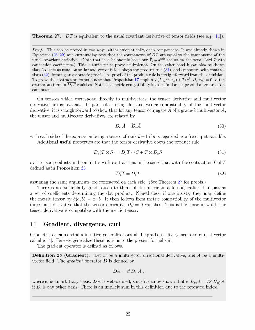
Theorem 27. DT is equivalent to the usual covariant derivative of tensor fields (see e.g. [11]).

Proof. This can be proved in two ways, either axiomatically, or in components. It was already shown inEquations (28–29) and surrounding text that the components of DT are equal to the components of theusual covariant deriative. (Note that in a holonomic basis our Γijmgmk reduce to the usual Levi-Civitaconnection coefficients.) This is sufficient to prove equivalence. On the other hand it can also be shownthat DT acts as usual on scalar and vector fields, obeys the product rule (31), and commutes with contrac-tions (32), forming an axiomatic proof. The proof of the product rule is straightforward from the definition.To prove the contraction formula note that Proposition 17 implies T (Deie

k, ek) + T (ek, Deiek) = 0 so theextraneous term in DaT vanishes. Note that metric compatibility is essential for the proof that contractioncommutes.

On tensors which correspond directly to multivectors, the tensor derivative and multivectorderivative are equivalent. In particular, using dot and wedge compatibility of the multivectorderivative, it is straightforward to show that for any tensor conjugate A of a grade-k multivector A,the tensor and multivector derivatives are related by

Da A = DaA (30)

with each side of the expression being a tensor of rank k+1 if a is regarded as a free input variable.Additional useful properties are that the tensor derivative obeys the product rule

Da(T ⊗ S) = DaT ⊗ S + T ⊗DaS (31)

over tensor products and commutes with contractions in the sense that with the contraction T of Tdefined as in Proposition 23

DaT = DaT (32)

assuming the same arguments are contracted on each side. (See Theorem 27 for proofs.)There is no particularly good reason to think of the metric as a tensor, rather than just as

a set of coefficients determining the dot product. Nonetheless, if one insists, they may definethe metric tensor by g(a, b) = a · b. It then follows from metric compatibility of the multivectordirectional derivative that the tensor derivative Dg = 0 vanishes. This is the sense in which thetensor derivative is compatible with the metric tensor.

11 Gradient, divergence, curl

Geometric calculus admits intuitive generalizations of the gradient, divergence, and curl of vectorcalculus [4]. Here we generalize these notions to the present formalism.

The gradient operator is defined as follows.

Definition 28 (Gradient). Let D be a multivector directional derivative, and A be a multi-vector field. The gradient operator D is defined by

DA = eiDeiA ,

where ei is an arbitrary basis. DA is well-defined, since it can be shown that eiDeiA = Ej DEjA

if Ei is any other basis. There is an implicit sum in this definition due to the repeated index.

22

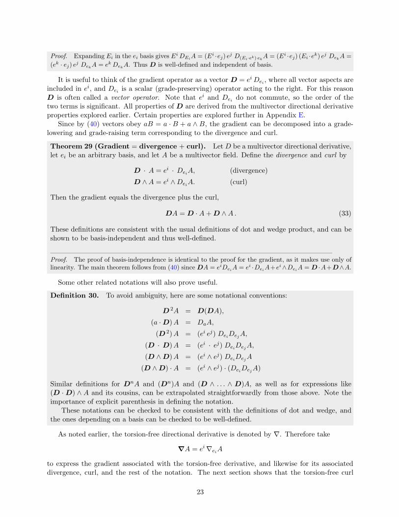
Proof. Expanding Ei in the ei basis gives EiDEi

A = (Ei ·ej) ej D(Ei·ek) ekA = (Ei ·ej) (Ei ·e

k) ej DekA =

(ek · ej) ej DekA = ek DekA. Thus D is well-defined and independent of basis.

It is useful to think of the gradient operator as a vector D = ei Dei , where all vector aspects areincluded in ei, and Dei is a scalar (grade-preserving) operator acting to the right. For this reasonD is often called a vector operator. Note that ei and Dei do not commute, so the order of thetwo terms is significant. All properties of D are derived from the multivector directional derivativeproperties explored earlier. Certain properties are explored further in Appendix E.

Since by (40) vectors obey aB = a · B + a ∧ B, the gradient can be decomposed into a grade-lowering and grade-raising term corresponding to the divergence and curl.

Theorem 29 (Gradient = divergence + curl). Let D be a multivector directional derivative,let ei be an arbitrary basis, and let A be a multivector field. Define the divergence and curl by

D · A = ei · DeiA, (divergence)

D ∧A = ei ∧DeiA. (curl)

Then the gradient equals the divergence plus the curl,

DA = D ·A+D ∧A . (33)

These definitions are consistent with the usual definitions of dot and wedge product, and can beshown to be basis-independent and thus well-defined.

Proof. The proof of basis-independence is identical to the proof for the gradient, as it makes use only oflinearity. The main theorem follows from (40) since DA = eiDeiA = ei ·DeiA+ei∧DeiA = D ·A+D∧A.

Some other related notations will also prove useful.

Definition 30. To avoid ambiguity, here are some notational conventions:

D 2A = D(DA),

(a ·D)A = DaA,

(D 2)A = (ei ej) DeiDejA,

(D · D)A = (ei · ej) DeiDejA,

(D ∧D)A = (ei ∧ ej) DeiDejA

(D ∧D) ·A = (ei ∧ ej) · (DeiDejA)

Similar definitions for DnA and (Dn)A and (D ∧ . . . ∧ D)A, as well as for expressions like(D ·D) ∧ A and its cousins, can be extrapolated straightforwardly from those above. Note theimportance of explicit parenthesis in defining the notation.

These notations can be checked to be consistent with the definitions of dot and wedge, andthe ones depending on a basis can be checked to be well-defined.

As noted earlier, the torsion-free directional derivative is denoted by ∇. Therefore take

∇A = ei∇eiA

to express the gradient associated with the torsion-free derivative, and likewise for its associateddivergence, curl, and the rest of the notation. The next section shows that the torsion-free curl

23

associated with this gradient is closely related to the exterior derivative of differential forms. Therelation of∇∧ to the usual curl from vector calculus, as well as some more properties of the gradient,are also given at the end of the next section.

12 Differential forms, exterior derivative

The space of differential forms (totally antisymmetric tensors) has an equivalent structure to theexterior subalgebra of multivector fields. In particular, the tensor conjugate map A 7→ A defined inSection 9 provides a bijection from multivectors to forms. Here we investigate this correspondencein more detail, and show that the theory of differential forms is fully included within the presentmethods.

For reasons to be justified shortly, define the exterior derivative d = ∇∧ as the torsion-free curl.

Definition 31 (Exterior derivative). Define the exterior derivative d of a multivector A by

dA = ∇ ∧A .

That is, the exterior derivative d is equivalent to the torsion-free curl.

When acting on scalar fields ϕ the exterior derivative

dϕ = ∇ ∧ ϕ = ∇ϕ = ei ∂eiϕ (34)

is merely the usual gradient. More generally, the exterior derivative has a simple expression whengeneral multivectors are expressed in a gradient basis. In particular, in terms of the coordinategradient basis dxi for a coordinate system xi the exterior derivative of an arbitrary multivector fieldA =

∑J AJ dx

J evaluates to

dA =∑

J

dAJ ∧ dxJ (35)

where as usual dxJ is the multivector basis constructed by wedging the vector basis dxi. Thisformula is proved within the proof of Corollary 33 below. In any basis which is not a gradient basisthe expression of dA does not have such a simple form.

The exterior derivative has some important properties.

Theorem 32 (Exterior derivative properties). The exterior derivative d = ∇∧ of multi-vectors has the following properties:

(i) d(A+B) = dA+ dB.

(ii) If ϕ is a scalar field then a · dϕ = ∂aϕ for all vector fields a.

(iii) If ϕ is a scalar field then d2ϕ ≡ d(dϕ) = 0.

(iv) If Aj and Bk are multivectors of fixed grades j and k respectively, then

d(Aj ∧Bk) = d(Aj) ∧Bk + (−1)j Aj ∧ d(Bk) .

Proof. (i) Trivial. (ii) a · dϕ = a · ei ∂eiϕ = ∂aϕ. (iii) Choose to work in a holonomic coordinatebasis ei = e(xi) so that Lijk = 0. Note that in this basis ei ∧ ∇eie

j = −Γilmgmj(ei ∧ el) = 0 since(ei ∧ el) = −(el ∧ ei) and by torsion-freeness Γilm − Γlim = Lilm = 0. Similarly note that in this basis(ei ∧ ej)∂ei∂ejϕ = 0 since coordinate partial derivatives commute. Thus d2ϕ = ei ∧ ∇ei(e

j∂ejϕ) = (ei ∧∇eie

j)∂ejϕ + (ei ∧ ej)∂ei∂ejϕ) = 0. (iv) Note that ei ∧ Aj = (−1)j(Aj ∧ ei) since the wedge product

24

commutes under vector swaps. Thus (suppressing grade labels) d(A ∧B) = ei ∧ (∇eiA ∧B+A∧∇eiB) =dA ∧B + ei ∧A ∧ ∇eiB = dA ∧B + (−1)jA ∧ dB.

Note that the torsion-free assumption was essential in the proof of (iii). Also, together theseconditions are sufficient to prove an additional property.

Corollary 33 (Exterior derivative properties). The above properties also imply that

(v) On any multivector field A

d2A = ∇ ∧ (∇ ∧A) = 0 .

Proof. Choose to work in the gradient basis dxi ≡ ∇ ∧ xi associated with a coordinate system xi (seeSection 4). Any A can be expanded A =

∑J AJ ∧ dxJ where AJ are scalar components. Then dA =∑

J (dAJ ∧ dxJ +AJ ∧ d(dx

J )) by properties (i,iv). But d(dxJ ) = d(dxj1 ∧ . . .∧ dxjN ) = 0 using properties(iv,iii) since each dxi has the form dϕ. Thus dA =

∑J(dAJ ∧ dxJ ). Applying the same logic again, one

then finds d2A =∑

J (d2AJ ∧ dxJ ) = 0, since AJ are scalars as noted before.

The properties (i-v) are precisely the defining properties of the exterior derivative in differentialforms! (See, e.g., [10] for a standard treatment.) Conceptually, this is sufficient to make theidentification between d = ∇∧ and the usual exterior derivative of differential forms.

This equivalence is made rigorous by the following theorem.

Theorem 34 (Equivalence of forms to multivectors). The tensor conjugate map A 7→ A(see Section 9) is a bijection from multivectors to differential forms which preserves the linear,exterior, and differential structures, in the sense that

(i) αA+ βB∧

= αA+ βB.

(ii) A ∧B = A ∧ B,

(iii) dA = dA.

Note that d is the exterior derivative of differential forms, while d is the exterior derivative ofmultivectors. Differential form definitions may be found in [10].

Proof. Since forms, unlike tensors, technically allow the formal sum of different signatures, the tensor con-

jugate mapping for present purposes should be extended to A =∑

k 〈A〉k, with the k-form Ak(a1, . . . , ak) =Ak · (a1 ∧ . . . ∧ ak) as defined previously, where we’ve replaced Ak ≡ 〈A〉k for notational convenience.Clearly the image of Ak is a totally antisymmetric tensor, so the image of A is a form. It is trivialto show (i) using linearity of the grade operator and dot product. To proceed, introduce a coordinate

system xi with coordinate basis e(xi) and reciprocal basis dxi in the multivector sense. The image dxi

is equivalent to the differential form dxi since dxi(e(xj)) = dxi · e(xj) = δij = dxi(e(xj)). Now let

dxJ = dxjr ∧ . . . ∧ dxj1 . Using Equation (4.12) of [2] and Proposition 14.11e of [10], it follows that

dxJ (a1, . . . , ar) = (dxjr ∧ . . . ∧ dxj1 ) · (ak1∧ . . . ∧ akr

) = det(dxj · ak) = det(dxj(ak)) = dxJ (a1, . . . , ar).

In other words, the multivector basis elements dxJ map to the form basis dxJ . Thus, using linearity, ifA =

∑K AKdxK then A =

∑K AK dxK . This formula makes it clear that the map is a bijection, since

A = 0 implies AK = 0 implies A = 0, and the form with arbitrary coefficients AK is mapped to by themultivector with equal coefficients. It remains to show (ii) and (iii). For (ii), the same logic as above shows

that dxJ ∧ dxK∧

= dxJ ∧ dxK . Thus A ∧B =∑

JK AJBKdxJ ∧ dxK∧

= A∧ B. Then (iii) also follows, since

25

dA =∑

K dAK ∧ dxK∧

=∑

K dAK ∧ dxK =

∑K ∂iAK dxi ∧ dxK = dA using Theorem 14.24 of [10] for the

final step.

This shows that the theory of multivector fields includes the the theory of differential forms asa part of a more general theory.

A corollary of this equivalence is that the multivector exterior derivative d = ∇∧ is independentof the metric, since it is equivalent to the exterior derivative of differential forms (which is definedwithout reference to a metric). This fact is somewhat surprising, since the directional derivative ∇underlying d is metric-compatible.

Geometric algebra also has an equivalent of the Hodge dual of differential forms: the multivectordual. The dual A∗ of a multivector A is defined by A∗ = AI−1, where I is an oriented unitpseudoscalar [4]. The dual of a k-vector Ak is an (N − k)-vector representing the orthogonalcomplement of Ak, where N is the total dimension of the space. The multivector dual has theimportant properties (A ·B)∗ = A ∧B∗ and (A ∧B)∗ = A ·B∗ and 0∗ = 0 [4]. The dual operationcan be used to investigate in more detail the relation between geometric calculus and differentialforms.

The quantity ∇ × a which in three-dimensional vector calculus is usually called the curl of avector field a is related to the multivector curl by duality: ∇× a = (∇ ∧ a)∗. In three dimensionsthis returns a vector orthogonal to the plane of the bivector ∇ ∧ a.

A useful consequence of the properties of duality is that d2 = 0 implies ∇ · (∇ · A) = 0 inaddition to ∇∧(∇∧A) = 0, so that ∇2 is in general a grade-preserving operator. Duality relationsalso show that the differential forms codifferential δA ≡ ∗ d ∗A = ∇ ·A is equivalent to divergence.

13 Concluding remarks

This article has attempted to lay an elementary foundation for studying geometric calculus onpseudo-Riemannian manifolds. The framework was seen to provide conceptually simple proofs ofmany concepts, such as obtaining a simple derivation of the Levi-Civita coefficients in arbitrarynon-holonomic bases, demonstrating how the tensor covariant derivative follows from a chain rule,and clarifying the importance of gradient bases as the reciprocal to holonomic bases. We rederivedthese known concepts within a new constructive framework—an axiomatic formalism more similarto standard Riemannian geometry and general relativity than existing treatments. We hope thiscan serve both as a pedagogical introduction to the topic, and as a useful bridge for physicists toapply geometric calculus concepts in the context of relativity.

Acknowledgements

I would like to thank Anthony Aguirre, Adam Reyes, and Ross Greenwood for useful discussions,and to thank David Constantine for first teaching me Riemannian geometry. This research wassupported by the Foundational Questions Institute (FQXi.org), of which AA is Associate Director,and by the Faggin Presidential Chair Fund.

26

A Geometric algebra review

Here we provide a basic review of geometric algebra (GA), both as an introduction and to setnotation. For more detailed reviews, there are a number of useful options: the books and surveyby Macdonald [4, 13, 14] give a clear and basic introduction, the book by Doran and Lasenby [3]highlights many applications to physics, and the original monograph by Hestenes and Sobczyk [2]provides a more complete theoretical development. These each use somewhat different conventions,but are still mutually intelligible. Conventions here are in line with Macdonald.

The basic objects of geometric algebra are multivectors, which can be visualized as (sums of)k-dimensional parallelepipeds sitting in N -dimensional space. These parallelepipeds range fromdimension zero (scalars), and one (vectors), up to N , the dimension of the ambient space. Inthis way multivectors provide a natural way to represent oriented lengths, areas, and volumes inphysical space. Geometric algebra is also known as Clifford algebra (Clifford himself used the formername [1]), and it includes exterior algebra as a sub-algebra under the wedge product.

In more detail, a geometric algebra is a linear space which can be built on top of an innerproduct vector space, by adding in the additional operation of wedge multiplication. The dot(inner) product

a · b

of vectors is a scalar, while the wedge (outer) product

a ∧ b

of two vectors is a new type of object called a 2-vector. In GA scalars (0-vectors), vectors (1-vectors),2-vectors (also called bivectors), and higher order k-vectors (formed by additional wedging, and vi-sualized as k-dimensional parallelepipeds) are all a part of the same linear space, which is calledthe space of multivectors. The order k of a k-vector is called its grade, and k-vectors of differentgrade are linearly independent from one another. The wedge product is antisymmetric on vec-tors and associative on all multivectors (thus totally antisymmetric under vector swaps), so thatk-vectors a1 ∧ . . . ∧ ak can be formed all the way up to the dimension N of the vector subspace. Anessential aspect of GA is that k-vectors can be linearly independently added, so that an arbitrarymultivector is written

A =

N∑

k=0

〈A〉k , (36)

where 〈〉k is called the grade operator, which picks out the k-vector part of a multivector. Whendifferent grades are added together they do not combine, and should be visualized as the formal sumof two separate parallelepipeds. The ability to add together different grades is leveraged to combinethe dot and wedge products into a more fundamental operation called the geometric product, whichacts on vectors a and b by

ab = a · b+ a ∧ b, (37)

so that the geometric product ab of two vectors is equal to a scalar plus a 2-vector. More generally,the geometric product of arbitrary of multivectors is written

AB

and from a technical perspective is considered the fundamental operation of GA (not derivable fromother operations, an elementary construction is given by [16]). The geometric product is associativeand distributes over addition, but is not commutative. The dot and wedge products for general

27

multivectors, meanwhile, are defined in terms of the geometric product. For pure-grade multivectorsAj (a j-vector) and Bk (a k-vector) the dot and wedge are defined by

Aj · Bk = 〈AjBk〉 k−j ,

Aj ∧Bk = 〈AjBk〉 k+j ,(38)

so that the dot (wedge) product acts as the maximally-grade-lowering (maximally-grade-raising)component of the geometric product. This definition is extended to arbitrary multivectors, whichcan be written as sums of pure-grade multivectors, by linearity. On vectors the dot and wedgeamount to

a · b = (ab+ ba)/2 ,

a ∧ b = (ab− ba)/2 ,(39)

which could also be derived from the earlier expression for ab using a · b = b · a and a ∧ b = −b ∧ a.There is another useful identity for vectors [4], written

aB = a ·B + a ∧B, (40)

but in generalAB 6= A · B +A ∧B . (41)

There is no need to introduce a basis to work in GA, since one typically works directly withvectors and multivectors, rather than with components. But introducing a basis is sometimes useful.One typically starts with a vector basis ei which can be extended to a canonical multivector basis eJby wedging the vector basis elements (more details below in the discussion of geometric manifolds).Every vector basis ei has a unique reciprocal basis ei such that

ei · ej = δij .

Which one has the upper and which one has the lower index is arbitrary, this is simply a pairof two vector basis sets which are mutually reciprocal. Reciprocality is a property of basis sets,and there is no such thing as the reciprocal of an individual vector (although a vector does havereciprocal components a = ai ei = ai e

i relative to a pair of reciprocal bases). Even when a basis isintroduced, all expressions in GA are independent of the basis choice. For example a vector a canbe decomposed with respect to two different bases ei and ei in the same equation without confusion,

a = (a · ei) ei = (a · ei) ei

= ai ei = ai ei ,

as the equation itself is independent of any basis choice. The concept of “change of basis” is notparticularly important in the GA formalism, but if one desires to do so, one writes, for example,

a = ai ei = ai (ei · ej) ej = aj ej

to go from basis ei to basis ei. Components are used, but they are never removed from the context ofwell-defined expressions, where they always explicitly multiply basis vectors. Equalities are alwayswritten as equalities of multivectors and not equalities of components.

The possibility of adding together multivectors of various grades, combined with the identifica-tion of the geometric product as the fundamental type of multiplication, makes GA an especiallyuseful framework in physics, geometry, and calculus [3, 4].

28

B Smooth tangent structure

To ensure a suitable smooth structure for GTpM it must be constructed in terms of a coordi-nate system xi with coordinate tangent basis e(xi). In terms of this basis the metric coefficientse(xi) · e(xj) = gij must be smooth coefficients forming a symmetric invertible matrix (with smoothinverse coefficients gij defined by gijgjk = δik) at each point.

The coordinate vector basis e(xi) (denote e(xi) ≡ Ei for convenience) generates a canonicalmultivector basis at each point in the following standard way. Let J be a (nonrepeating, unordered)set of valid indices for Ei. Denote by EJ the wedge product

EJ = Ej0 ∧ . . . ∧ Ejn (42)

with the product taken over all ji ∈ J , such that the indices ji strictly increase towards the right(when J is the empty set EJ = 1). The set of EJ for all index sets J forms a basis for multivectorsin GTpM . Every multivector field A can be uniquely expressed in the canonical coordinate basisby

A = AJEJ (43)

where AJ are scalar field coefficients. A multivector field is considered smooth when the coefficientsAJ are smooth in the multivector coordinate basis. This implies that a vector field a is smooth ifand only if the scalar fields (a ·Ei) are smooth.

Consider a collection of vector fields ei which form a basis for TpM at each point. There existsat each point a reciprocal basis ei such that ei · ej = δij . These ei are a smooth (vector) basis frame

(or smooth basis vector fields) if the scalar fields (ei ·Ej) and (ei ·Ej) are all smooth relative to the

coordinate basis.A smooth vector frame generates a multivector frame eJ = ej0 ∧ . . . ∧ ejn analogous to the

canonical coordinate frame above, and every multivector field has a unique expression B = BJeJin this frame. Under the the given definitions, it can be shown that multivector fields are smoothif and only if their coefficients are smooth in the eJ basis for any smooth vector frame ei.

C Proof of Theorem 11 (MDD preserves grade)

Let D be a directional derivative, and let Ei be an orthonormal basis with associated multivectorbasis EJ . It suffices to show that DEi

EJ is grade-preserving for all basis vectors Ei and basismultivectors EJ . The proof follows from a simple pattern, where potentially non-grade-preservingterms come in pairs which together vanish by metric compatibility, but there is no simple notationto show the proof algebraically. The pattern can quickly be observed by calculating DEi

(E1E2E3)and DEi

(E1E2E3E4) in the orthonormal basis, in which examples the non-grade-preserving term isseen to explicitly vanish. The pattern generalizes as follows.

Since the basis is orthonormal, Ei = ±Ei and EiEi = 1, and j 6= k implies EjEk = −EkEj . An

arbitrary multivector basis element of grade n can be written EJ = Ej1 . . . Ejn , where j1 < . . . < jn.Consider the first term DEi

(Ej1) . . . Ejn in the product rule expansion for DEiEJ . Decompose the

derivative into components in the Ek basis to write this term as

∑k(DEi

(Ej1) · Ek)Ek . . . Ejn .

Since Ek = ±Ek is orthogonal to Ej whenever k 6= j, this term has grade n for all terms inthe sum where k /∈ (j2, . . . , jn). Every term which does not preserve grade has k = jp for somejp ∈ (j2, . . . , jn), in which case anticommuting Ek through basis vectors and utilizing EkEjp = 1

29

leaves a constant times the multivector term EJ with both E1 and Ejp removed. Thus every termeither has grade n or grade n − 2, and the terms with grade n − 2 are proportional to EJ withtwo basis vectors removed from the product. This generalizes to every term in the product ruleexpansion, so to show that grade is preserved one must show that the total grade n− 2 term in theproduct rule expansion vanishes.

Denote by J(p, q) the set of indices (j1, . . . , jn) with jp and jq removed. The preceding paragraphimplies that DEi

EJ = 〈DEiEJ〉n+ 〈DEi

EJ〉n−2 where 〈DEiEJ〉n−2 =

∑(p,q)A

J(p,q)EJ(p,q). We now

show that AJ(p,q) = 0 using metric compatibility.Consider DEi

(Ej1 . . . Ejp . . . Ejq . . . Ejn). Every term in the product rule expansion which doesnot take a derivative of either Ejp or Ejq does not contribute to EJ(p,q), since it can only eliminate oneor the other of the two factors. Two terms remain. The p derivative term is

∑k Ej1 . . . (DEi

(Ejp) ·Ek)E

k . . . Ejq . . . Ejn . This contributes to EJ(p,q) only for k = q. The q derivative term is analogous,so that the total EJ(p,q) term is

(Ej1 . . . (DEi

(Ejp) · EJq)Ejq . . . Ejq . . . Ejn

)+

(Ej1 . . . Ejp . . . (DEi

(Ejq ) · Ejp)EJp . . . Ejn

).

Commuting scalars and anticommuting basis vectors makes this term equal to

(−1)(q−p−1)[DEi

(Ejp) · Ejq +DEi(Ejq) ·Ejp

]EJ(p,q).

Thus by metric compatibility AJ(p,q) = ±DEi(Ejp · Ejq) = 0 since the basis is orthonormal.

Since every term proportional to EJ(p,q) is zero, and every other term in the product ruleexpansion preserves grade, the derivative obeys 〈DEi

〈EJ〉n〉n = DEi〈EJ 〉n. Extending this result to

arbitrary multivectors by linearity and the properties of D implies that the directional derivativepreserves the grade of all multivectors.

D Proof of Theorem 14 (MDDs↔metric-compatible connections)

We must show that for any metric-compatible affine connection D, there exists a multivector di-rectional derivative operator D which restricts to D when acting on vector fields. We achieve thisby directly constructing an operator D that restricts to D, then showing that D is an MDD by theaxioms of Definition 8.

D is constructed by defining its action on multivectors in a particular basis. Throughout theproof, Ei refers to the specific orthonormal basis in terms of which D is defined. Likewise, EJ isthe canonical multivector basis constructed from Ei.

Definition 35. Let D be a metric-compatible affine connection. Let Ei be a set of smoothorthonormal basis vector fields with associated canonical multivector basis EJ . Every smoothmultivector field can be written uniquely in the form A =

∑J A

JEJ , where AJ are smooth scalar

field coefficients. Define an operator D : TpM ×MVF (M)→ GTpM by

30

(i) D(α a+β b)A = αDaA+ β DbA,

(ii) DEi(1) = 0,

(iii) DEi(Ej) = DEi

(Ej),

(iv) Da(∑

J AJEJ) =

∑J

((∂aA

J )EJ +AJ (DaEJ)),

(v) For EJ with grade greater than one, Da(EJ ) defined by the product rule:

If i < k for all k ∈ K, then Da(EiEK) = (DaEi)EK +Ei(DaEK).

This suffices to uniquely define the operator D on all smooth multivector fields, and D restrictsto D when acting on vector fields.

This D is a well-defined operator which is equal to the metric-compatible affine connection Dwhen restricted to act on vector fields. If D satisfies all the axioms of Definition 8, then D is amultivector directional derivative. All the axioms except the product rule come easily.

Lemma 36. D satisfies properties (i-iv) of Definition 8.

Proof. (i) True by assumption. (ii) Let 〈A〉0 = ϕ. Then Da〈A〉0 = Da(ϕ1) = (∂aϕ)1 + ϕ(Da1) = ∂aϕ =∂a〈A〉0. (iii) Let 〈A〉1 = bjEj . Then Da〈A〉1 = Da(b

jEj) = ai(∂Eibj)Ej + aibj(DEi

Ej) = ai(∂Eibj)Ej +

aibjγijkEk, which is a vector. (iv) Da(A + B) = Da(A

JEJ + BJEJ ) = Da((AJ + BJ )EJ ) = ∂a(A

J +BJ)EJ + (AJ +BJ)DaEJ = DaA+DaB.

Thus if D obeys the product rule then it is a multivector directional derivative.The MDD axioms imply metric-compatibility on vectors. It follows that if D were not metric-

compatible, then D would have to violate the product rule. But D is metric-compatible, and itturns out this is sufficient to ensure the product rule is obeyed by D. The method of proof is toshow that the product rule holds as a special case for increasingly general strings of the orthonormalbasis vectors Ei in terms of which the action of D is defined.

First, a product rule is shown for pairs of basis vectors.

Lemma 37. On a pair of the defining basis vectors

DEi(EjEk) = (DEi

Ej)Ek + Ej(DEiEk) .

Proof. Define DEiEj = γijkE

K . Since D is metric-compatible and Ei orthonormal, γijk + γikj = 0. Theproof follows from showing that DEi

(EjEk) − (DEiEj)Ek − Ej(DEi

Ek) = 0. There are three cases. For(j < k), the product rule is assured by definition ofD. For (j = k), DEi

(EjEj)−(DEiEj)Ej−Ej(DEi

Ej) =0 − 2(DEi

Ej) · Ej = −2γijj = 0. For (j > k), one finds DEi(EjEk) − (DEi

Ej)Ek − Ej(DEiEk) =

−DEi(EkEj) − (DEi

Ej)Ek − Ej(DEiEk) = −(DEi

Ek)Ej − Ek(DEiEj) − (DEi

Ej)Ek − Ej(DEiEk) =

−2(DEiEj) ·Ek − 2(DEi

Ek) ·Ej = −2(γijk + γikj) = 0.

This can be extended from pairs of basis vectors to strings of basis vectors.

Lemma 38. Say that an arbitrary string Ej1 . . . Ejn of n of the defining basis vectors is product-rule-separable if it splits into derivatives of individual basis vectors in the usual way:

DEi(Ej1 . . . Ejn) = (DEi

Ej1)Ej2 . . . Ejn + . . .+ Ej1 . . . Ejn−1(DEi

Ejn).

Then product rule separability of basis strings is preserved by the basic manipulations of neighbor-swapping and pair insertion. That is, if ǫ = Ej0 . . . EjmEjm+1

. . . Ejn is product-rule-separable,

31

then

(i) ǫ′ = Ej0 . . . Ejm+1Ejm . . . Ejn is product-rule-separable,

(ii) ǫ′′ = Ej0 . . . EjmEkEkEjm+1. . . Ejn is product-rule-separable, for any Ek.

Proof. (i) If Ejm = Ejm+1then ǫ′ = ǫ which is separable. Otherwise, DEi

ǫ′ = DEi(−ǫ) = −DEi

ǫ.One can show that −DEi

ǫ is equal to the product rule expansion for ǫ′. Expand DEiǫ by the prod-

uct rule. The product rule expansion for ǫ′ is obtained by swapping m ↔ m + 1 in each term. Thisyields a negative sign in each term, seen as follows. For each term with EmEm+1 outside the deriva-tive, the identity EjEk = −EkEj for j 6= k suffices to give the negative sign. The two remaining termsare of the form A[(DEi

Em)Em+1 + Em(DEiEm+1)]B = A(DEi

(EmEm+1))B = A(DEi(−Em+1Em))B =

−A(DEi(Em+1Em))B = −A[(DEi

Em+1)Em +Em+1(DEiEm)]B, using the product rule proved earlier for

pairs of basis vectors, which yields the desired negative sign. Thus DEiǫ′ is equal to its product rule

expansion. (ii) DEiǫ′′ = DEi

(E2kǫ) = E2

kDEiǫ since E2

k is a constant scalar. Expand E2kDEi

ǫ by the prod-uct rule. For every term with no derivatives of Ek, the scalar E2

k can be freely moved between Em andEm+1. The remaining two terms are obtained by adding in a term of the form 0 = A(DEi

(EkEk))B =A[(DEi

Ek)Ek + Ek(DEiEk)]B using the product rule for pairs of basis vectors. Thus E2

kDEiǫ is equal to

the product rule expansion of DEiǫ′′.

Using these operations, product rule separability can be shown for arbitrary basis strings, whichimplies the product rule for arbitrary multivectors.

Lemma 39. It follows from the previous lemma that

(i) Every string of the basis vectors Ei is product-rule-separable,

(ii) DEi(EJEk) = (DEi

EJ)Ek + EJ(DEiEk) for all Ei, EJ , EK ,

(iii) Da(AB) = (DaA)B +A(DaB) for all a,A,B.

Proof. (i) Every EJ is product-rule-separable by definition of D. Every arbitrary string of basis vectorscan be formed from some EJ by a series of neighbor-swaps and pair-insertions. These operations preserveproduct-rule-separability as shown above. (ii) EJ , EK , and EJEK are all strings of basis vectors, and thuscan be expanded and recombined by their product rule expansions, as shown above. (iii) This follows fromthe definition of D from direct calculation of Da(AB) by expansion in the canonical basis, using additivityfrom Lemma 36 and the product rule for EJEk.

Thus it has been shown that D obeys the product rule and thus satisfies all axioms of Defini-tion 8. So for each metric compatible affine connection D, D is a multivector directional derivativerestricting to it. This concludes the proof.

It is worth noting that, so far, it seems that making fundamental use of the neighbor-swappingand pair insertion operations in an orthonormal canonical basis is the only reasonable way to attackthe above proof. Some time after reaching that conclusion, I found out that Alan Macdonald’s sim-plest “elementary construction” of GA [16] (which long precedes this work) is based on exactly thesame operations. This seems quite interesting, and points to the important role of these operationsunderlying the structure of GA.

E Gradient and linear transformations

Does the gradient operator encode all information about the directional derivative of a multivectorfield? No. This section explains why, by investigating similar operators in linear algebra.

32

Let A be a geometric algebra, and let f : 〈A〉1 → 〈A〉1 be a linear transformation of the vectorsubspace of A, so that for vectors a, b and scalars α, β,

f(αa+ βb) = αf(a) + βf(b).

Let ei be an arbitrary vector basis such that ei ·ej = gij , with reciprocal basis ei such that ei ·ej = δijand ei = gij ej , where gij is the matrix inverse to gij. By linearity f is determined by its scalarcomponents, defined by

f(ei) = fij ej = fi

j ej , f(ei) = f ij e

j = f ij ej ,

or equivalently by its vector components, defined by

f(ei) = fi , f(ei) = f i .

It follows from linearity that gij and its inverse can raise and lower each index of the components.Given f , define a multivector f by (with summation convention)

f = ei f(ei)

= ei · fi + ei ∧ fi

= tr(f) + rot(f)

where the trace tr(f) and rotation rot(f) of f are defined by

tr(f) = ei · f(ei) , rot(f) = ei ∧ f(ei) .

The trace is a scalar and the rotation is a bivector. In components,

f = f ij (gij + ei ∧ ej) , tr(f) = f ij gij , rot(f) = f ij ei ∧ ej .

The trace, rotation, and f can all be checked to be independent of what basis they are definedin. Note that the trace depends only on (f ij + f ji) and the rotation depends only on (f ij − f ji).Geometrically, the trace represents the average amount by which input vectors are scaled parallelto themselves by f , while the rotation encodes how much input vectors contribute to a componentpurely perpendicular to themselves.

The trace and rotation are best understood by noticing that every linear transformation admitsthe unique decomposition

f =(tr(f)n

)1+ f+ + f−

where 1 is the identity operator, n is the dimension of the space of vectors, and f± are tracelesssymmetric (+) and antisymmetric (−) linear transformations satisfying (f±(a) · b) = ± (a · f±(b))and tr(f±) = 0. This can be called the TSA (trace-symmetric-antisymmetric) decomposition.

Clearly tr(f) encodes the strength of the identity component in f . More surprising, perhaps, isthat the bivector rot(f) encodes the entirety of the antisymmetric part. In fact, for all a,

a · rot(f) = f−(a) .

It follows that in general

f(a) =(tr(f)n

)a+ a · rot(f) + f+(a) ,

33

and therefore that f = tr(f) + rot(f) encodes the 1 and f− parts of f but not the f+ part. Theremaining part f+ also admits a simple interpretation, since it can be shown that every symmetrictransformation has a basis of eigenvectors and obeys the spectral theorem [13]. Thus f+ is specifiedby a basis vi of eigenvectors and a set of eigenvalues λi, in terms of which

f+(a) =∑

i

λi (a · vi) vi .

Since f+ is traceless, the eigenvalues must sum to zero (∑

i λi = 0), which expresses in someheuristic sense that f+ is “conservative”.

To summarize, a linear transformation f is the sum of three basic operations. A trace term,characterized by a scalar tr(f), multiplies inputs by a constant scale factor. A rotation term,characterized by a bivector rot(f), returns a vector orthogonal to the input. And a traceless-symmetric term, characterized by an eigenbasis vi with eigenvalues λi summing to zero, scalesinputs along its characteristic directions. The multivector

f = ei f(ei) = tr(f) + rot(f)

encodes the trace and rotation terms, but not the traceless-symmetric term.For a fixed vector field b, the directional derivative f(a) = Dab is a linear transformation from

vectors to vectors. The gradient Db = eiDeib is exactly analogous to f for this transformation.The gradient of a vector field therefore encodes the trace (divergence) and rotation (curl) of thedirectional derivative, but ignores the traceless-symmetric part. This is specific to the gradient ofvector fields—for scalar fields the gradient encodes all information since Daϕ = a ·Dϕ, while forhigher grade fields the picture is more complicated.

References

[1] Professor Clifford. Applications of grassmann’s extensive algebra. American Journal of Math-ematics, 1(4):350–358, 1878.

[2] D. Hestenes and Garret Sobczyk. Clifford Algebra to Geometric Calculus: A Unified Languagefor Mathematics and Physics (Fundamental Theories of Physics). Springer, 1987.

[3] Chris Doran and Anthony Lasenby. Geometric Algebra for Physicists. Cambridge UniversityPress, 2007.

[4] Alan Macdonald. A survey of geometric algebra and geometric calculus. Advances in AppliedClifford Algebras, 27(1):853–891, Mar 2017.

[5] H. Blaine Lawson, Jr. and Marie-Louise Michelsohn. Spin geometry, volume 38 of PrincetonMathematical Series. Princeton University Press, Princeton, NJ, 1989.

[6] Albert Crumeyrolle. Orthogonal and symplectic Clifford algebras, volume 57 of Mathematicsand its Applications. Kluwer Academic Publishers Group, Dordrecht, 1990.

[7] Waldyr Alves Rodrigues, Jr. and Edmundo Capelas de Oliveira. The many faces of Maxwell,Dirac and Einstein equations, volume 722 of Lecture Notes in Physics. Springer, Berlin, 2007.

[8] David Hestenes and Garret Sobczyk. Clifford algebra to geometric calculus. FundamentalTheories of Physics. D. Reidel Publishing Co., Dordrecht, 1984.

34

[9] Chris Doran and Anthony Lasenby. Geometric algebra for physicists. Cambridge UniversityPress, Cambridge, 2003.

[10] John M. Lee. Introduction to Smooth Manifolds (Graduate Texts in Mathematics). Springer,2002.

[11] John M. Lee. Riemannian Manifolds: An Introduction to Curvature (Graduate Texts in Math-ematics). Springer, 1997.

[12] David Hestenes. Space-time algebra. Birkhauser/Springer, Cham, second edition, 2015.

[13] Alan Macdonald. Linear and Geometric Algebra. CreateSpace Independent Publishing Plat-form, 2011.

[14] Alan Macdonald. Vector and Geometric Calculus. CreateSpace Independent Publishing Plat-form, 2012.

[15] Bernard Schutz. Geometrical Methods of Mathematical Physics. Cambridge University Press,1980.

[16] Alan Macdonald. An elementary construction of the geometric algebra. Advances in AppliedClifford Algebras, 12(1):1–6, Jun 2002.

35