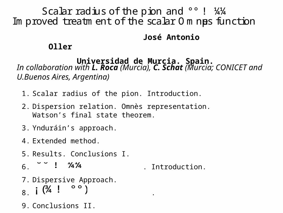
José Antonio Oller

Universidad de Murcia. Spain.

In collaboration with L. Roca (Murcia), C. Schat (Murcia; CONICET and U.Buenos Aires, Argentina)

Scalar radius of the pion and °° ! ¼¼Improved treatment of the scalar Omnµes function

1. Scalar radius of the pion. Introduction.

2. Dispersion relation. Omnès representation. Watson’s final state theorem.

3. Ynduráin’s approach.

4. Extended method.

5. Results. Conclusions I.

6. . Introduction.

7. Dispersive Approach.

8. .

9. Conclusions II.

°° ! ¼¼

¡ (¾! °°)

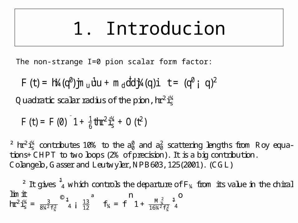
1. Introducion

F (t) = h¼(q0)jmu ¹uu+md¹ddj¼(q)i t = (q0¡ q)2

The non-strange I=0 pion scalar form factor:

Quadratic scalar radius of thepion, hr2i¼s

F (t) = F (0)©1+ 1

6thr2i¼s +O(t2)

ª

² hr2i¼s contributes 10% to the a00 and a20 scattering lengths from Roy equa-tions+CHPT to two loops (2% of precision). It is a big contribution.Colangelo, Gasser and Leutwyler, NPB603, 125(2001). (CGL)

² It gives ¹̀4 which controls thedeparture of F¼ from its value in the chirallimithr2i¼s =

38¼2 f 2¼

©¹̀4 ¡ 13

12

ªf¼= f

n1+ M 2

¼16¼2f 2¼

¹̀4

o

² One loop CHPT, Gasser and Leutwyler PLB125,325 (1983)hr2i¼s =0:55§ 0:15fm2

² Donoghue, Gasser, Leutwyler NPB343,341(1990) from thesolution of theMuskhelishvili-Omnµes (MO) equations, updated value in CGL.hr2i¼s =0:61§ 0:04 fm2

² Mousallam EPJ C14,11(200) allowed for two di®erent T¡ matrices in MOand obtained thesamevalues.

The scalar radius of thepion is noticeably larger than thecharged one,hr2¼i = 0:432§ 0:006 fm2

This is due to thepionic cloud (strong ¯nal state interactions)

MO equations have systematic uncertainties like their dependenceonvalues of strong amplitudes for non-physical values of energy.Assumptions on which are thechannels that matter.Multipion states areneglcted.Other approaches are then most welcome.

a00 =0:220§ 0:005 fm , a20 = ¡ 0:0444§ 0:0010 fm , precision 2%

This value ismuch larger than 0:61§ 0:04 fm2 and both are incompatible(less than 3%)

Consequences in the scattering lengths of CGL

Yall

² Elastic Omnµes representation and numerical-CHPT to two loopsGasser, Meissner NPB357,90(1991)

² Two-loop CHPT, Bijnens, Colangeloand Talavera JHEP 9805, 014 (1998)

² One loop UCHPT, Mei¼ner, JAO, NPA679, 671 (2001); Mei¼ner, Lahde,PRD74, 034021(2006)

² Yndur¶ain's approach based on the Omnµes representation of F (t)Yndur¶ain, PLB578, 99 (2004); (E)-ibid B586, 439 (2004) (Y1)Yndur¶ain, PLB612, 245 (2005) (Y2)Yndur¶ain, arXiv: hep-ph/0510317 (Y3)

hr2 i¼s =0:75± 0:07 fm2 \robust" lower bound: hr2 i¼s =0:70± 0:06 fm2

Mei¼ner

±a00 =+0:027¢ r 2 ±a20 = ¡ 0:004¢ r 2 hr2i¼s =0:61(1+¢ r 2 ) fm2

¢ r 2 =+0:23 between Yall and CGL±a00 =+0:006 and ±a20 = ¡ 0:001(in I=2 S-wave ¯nal state interactions aremuch smaller, exotic channel)The shift in thecentral value is onesigma of CGL

a00 =0:220§ 0:005 fm , a20 = ¡ 0:0444§ 0:0010 fm , precision 2%

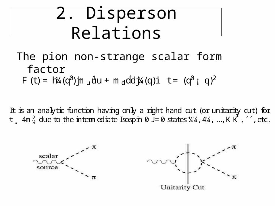
2. Disperson Relations

The pion non-strange scalar form factor

F (t) = h¼(q0)jmu ¹uu+md¹ddj¼(q)i t = (q0¡ q)2

It is an analytic function having only a right hand cut (or unitarity cut) fort ¸ 4m2

¼ due to the intermediate Isospin 0 J =0 states¼¼, 4¼, ..., K ¹K , ´´, etc.

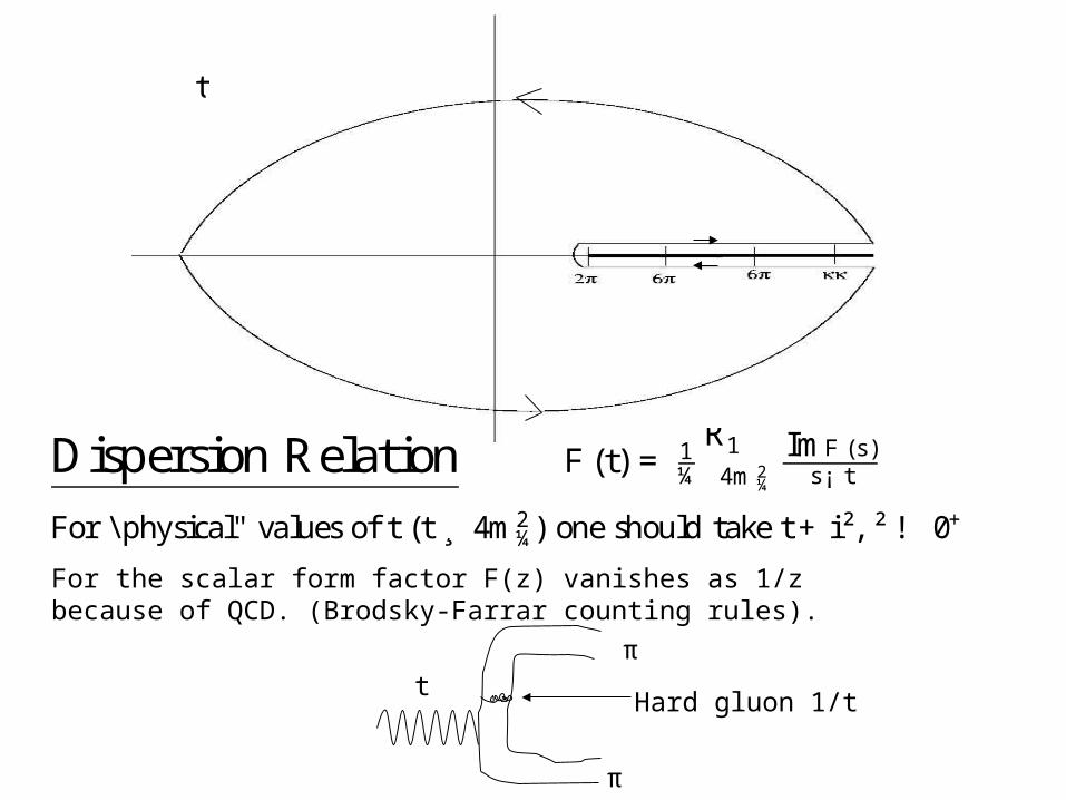
For \ physical" values of t (t ¸ 4m2¼) oneshould take t+ i², ² ! 0+

Dispersion Relation F (t) = 1¼

R14m2

¼

ImF (s)s¡ t

t

For the scalar form factor F(z) vanishes as 1/z because of QCD. (Brodsky-Farrar counting rules).

Hard gluon 1/tt

π

π

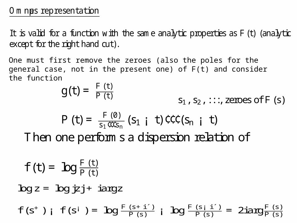
Omnµes representation

It is valid for a function with the same analytic properties as F (t) (analyticexcept for the right hand cut).

One must first remove the zeroes (also the poles for the general case, not in the present one) of F(t) and consider the function

g(t) = F (t)P (t)

P (t) = F (0)s1¢¢¢sn

(s1 ¡ t) ¢¢¢(sn ¡ t)

Then oneperforms a dispersion relation of

f (t) = log F (t)P (t)

logz = logjzj + iargz

f (s+) ¡ f (s¡ ) = log F (s+i´)P (s) ¡ log F (s¡ i´ )

P (s) = 2iargF (s)P (s)

s1, s2, : : :, zeroes of F (s)

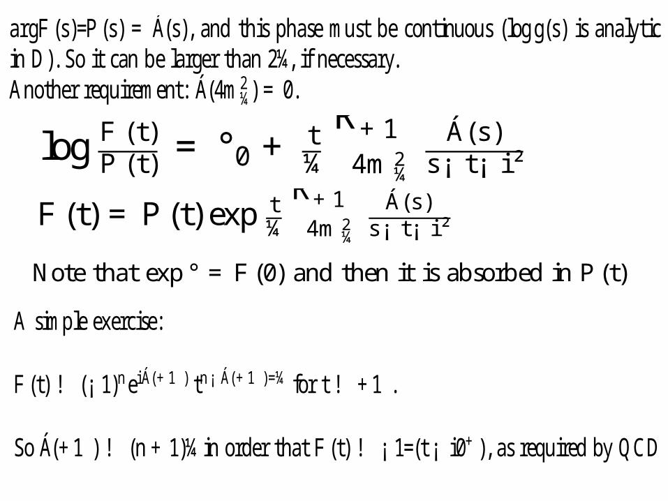
argF (s)=P (s) = Á(s), and this phasemust be continuous (logg(s) is analyticin D). So it can be larger than 2¼, if necessary.Another requirement: Á(4m2

¼) = 0.

A simple exercise:

F (t) ! (¡ 1)neiÁ(+1 ) tn¡ Á(+1 )=¼ for t ! +1 .

So Á(+1 ) ! (n+1)¼in order that F (t) ! ¡ 1=(t ¡ i0+), as required by QCD

F (t) = P (t) exp t¼

R+14m2

¼

Á(s)s¡ t¡ i ²

log F (t)P (t) = °0+ t

¼

R+14m2

¼

Á(s)s¡ t¡ i ²

Note that exp° = F (0) and then it is absorbed in P (t)

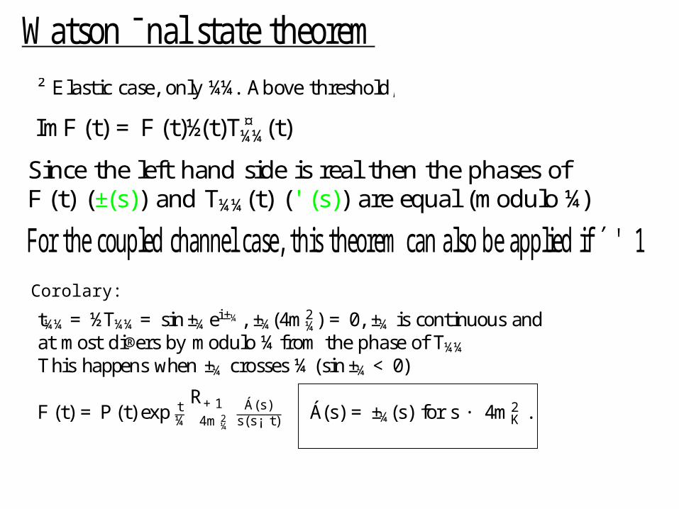
Watson ¯nal state theorem² Elastic case, only ¼¼. Above threshold,

ImF (t) = F (t)½(t)T¤¼¼(t)

Corolary:

For thecoupled channel case, this theoremcan also beapplied if ´ ' 1

t¼¼=½T¼¼= sin±¼ei±¼, ±¼(4m2¼) = 0, ±¼ is continuous and

at most di®ers by modulo ¼from thephaseof T¼¼This happens when ±¼ crosses ¼(sin±¼<0)

F (t) = P (t) exp t¼

R+14m2

¼

Á(s)s(s¡ t) Á(s) =±¼(s) for s · 4m2

K .

Since the left hand side is real then thephases ofF (t) (±(s)) and T¼¼(t) (' (s)) areequal (modulo¼)

3. Ynduráin’s method

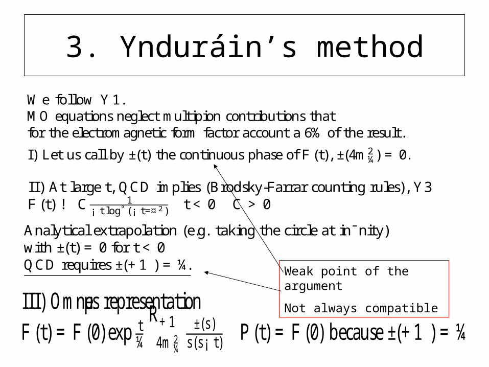
Analytical extrapolation (e.g. taking thecircleat in¯nity)with ±(t) = 0 for t < 0QCD requires ±(+1 ) =¼.

I I I) Omnµes representationF (t) = F (0) exp t

¼

R+14m2

¼

±(s)s(s¡ t) P (t) = F (0) because±(+1 ) =¼

I I) At large t, QCD implies (Brodsky-Farrar counting rules), Y3F (t) ! C 1

¡ t logº (¡ t=¤ 2) t < 0 C > 0

We follow Y 1.MO equations neglect multipion contributions thatfor theelectromagnetic form factor account a 6% of the result.

I) Let us call by ±(t) thecontinuous phaseof F (t), ±(4m2¼) = 0.

Weak point of the argument

Not always compatible

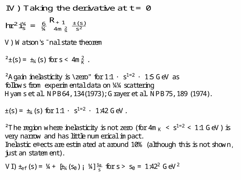
V) Watson's ¯nal state theorem

²±(s) =±¼(s) for s < 4m2K .

²Again inelasticity is \ zero" for 1:1 · s1=2 · 1:5 GeV asfollows fromexperimental data on ¼¼scatteringHyams et al. NPB64, 134(1973); Grayer et al. NPB75, 189 (1974).

±(s) =±¼(s) for 1:1 · s1=2 · 1:42GeV.

²The region where inelasticity is not zero (for 4mK < s1=2 <1:1GeV) isvery narrow and has littlenumerical impact.Inelastic e®ects areestimated at around 10% (although this is not shown,just an statement).

IV) Taking thederivativeat t = 0

hr2i¼s =6¼

R+14m2

¼

±(s)s2

VI) ±ef (s) =¼+[±¼(s0) ¡ ¼] s0s for s > s0 =1:422 GeV2

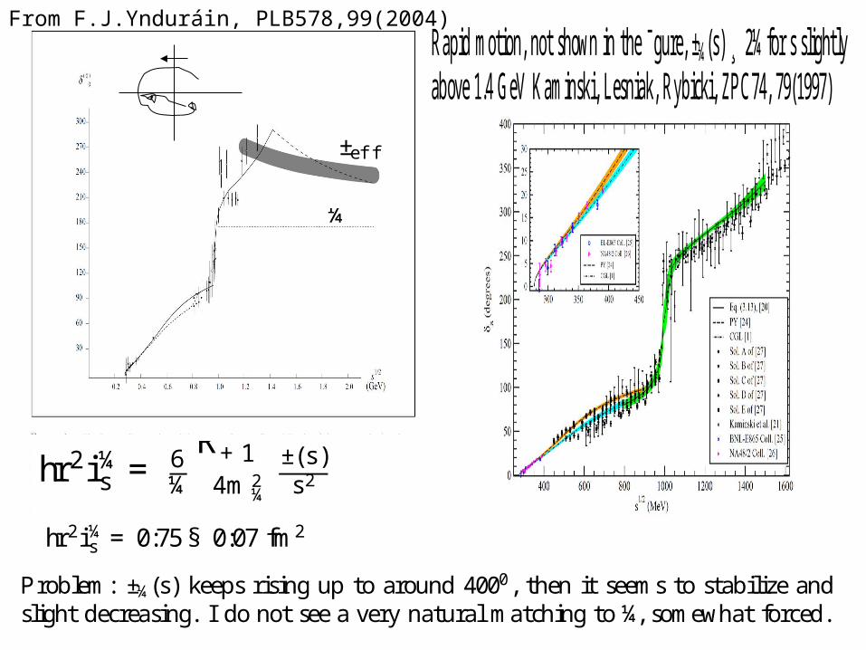
From F.J.Ynduráin, PLB578,99(2004)

hr2i¼s =0:75§ 0:07 fm2

±ef f

¼

Rapid motion, not shown in the ¯gure, ±¼(s) ¸ 2¼for s slightlyabove1.4GeV Kaminski, Lesniak, Rybicki, ZPC74, 79(1997)

hr2i¼s =6¼

R+14m2

¼

±(s)s2

Problem: ±¼(s) keeps rising up to around 4000, then it seems to stabilize andslight decreasing. I do not seea very natural matching to¼, somewhat forced.

This approach was critized by Ananthanarayan, Caprini, Leutwyler, IJMP A21,954 (2006) (ACGL).

Themain objection to thepreviousmethod is theway thattheWatson's ¯nal state theorem is applied in the regionabove theK K threshold.

It ¯xes thephasemodulo ¼, how can oneknow whether a °ip in ¼has not occured in the region between 2mK · s1=2 · 1:1 GeVwhere inelasticity is not zero?

ACGL concludesthat the§ ¼ambiguity in theWatson'stheoremcanberesolvedonly by explicit inclusion of inelastic channels in MO equations.

Thepoint is that 6¼

R ±¼(s)¡ ¼s2 ds above theK K threshold gives again

hr2i¼s ' 0:61 fm2.

They also mention other studies in which thepion scalar form factorhasaminimumjust below theK ¹K threshold and not thestrongmaximumthatY1 gives. (More later)

4. Extended Y’s method

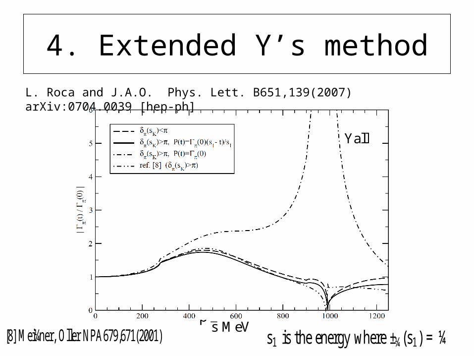
L. Roca and J.A.O. Phys. Lett. B651,139(2007) arXiv:0704.0039 [hep-ph]

Yall

[8] Mei¼ner, Oller NPA679,671(2001) s1 is theenergy where±¼(s1) =¼ps MeV

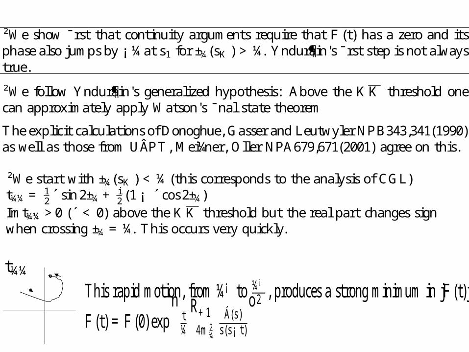
²Westart with ±¼(sK ) <¼(this corresponds to theanalysis of CGL)t¼¼= 1

2´ sin2±¼+i2(1¡ ´ cos2±¼)

Imt¼¼>0 (´ < 0) above theK K threshold but the real part changes signwhen crossing±¼=¼. This occurs very quickly.

This rapid motion, from¼¡ to ¼¡

2 , produces a strongminimum in jF (t)j

F (t) = F (0) expnt¼

R+14m2

¼

Á(s)s(s¡ t)

o

²We show ¯rst that continuity arguments require that F (t) has a zero and itsphasealso jumpsby ¡ ¼at s1 for ±¼(sK ) >¼. Yndur¶ain's¯rst step isnot alwaystrue.

²We follow Yndur¶ain's generalized hypothesis: Above the K K threshold onecan approximately apply Watson's ¯nal state theorem

Theexplicit calculationsof Donoghue, Gasser andLeutwyler NPB343,341(1990)as well as those fromUÂPT, Mei¼ner, Oller NPA679,671(2001) agreeon this.

t¼¼

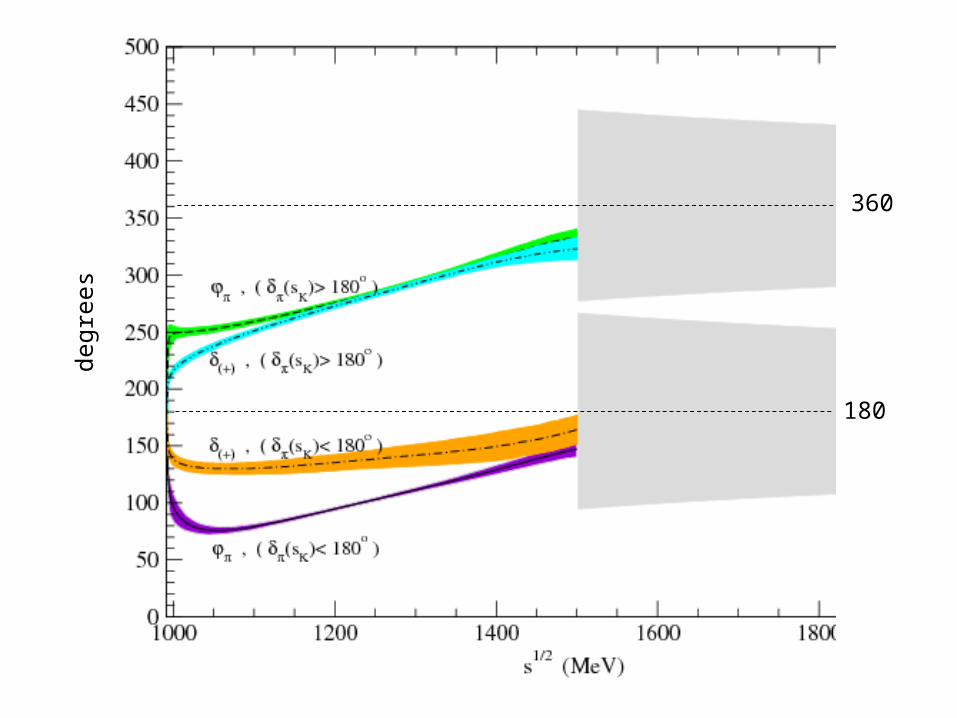
degr

ees

180

360

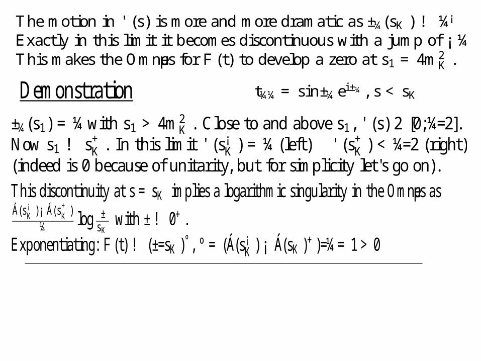
Themotion in ' (s) ismoreand moredramatic as ±¼(sK ) ! ¼¡

Exactly in this limit it becomes discontinuous with a jump of ¡ ¼This makes theOmnµes for F (t) to develop a zero at s1 =4m2

K .

Demonstration±¼(s1) =¼with s1 >4m2

K . Close to and aboves1, ' (s) 2 [0;¼=2].Now s1 ! s+K . In this limit ' (s

¡K ) =¼(left) ' (s+K ) <¼=2 (right)

(indeed is 0 becauseof unitarity, but for simplicity let's go on).

This discontinuity at s = sK implies a logarithmic singularity in theOmnµes asÁ(s¡K )¡ Á(s+K )

¼ log ±sK

with ±! 0+.Exponentiating: F (t) ! (±=sK )º , º = (Á(s¡K ) ¡ Á(sK )+)=¼=1> 0

t¼¼= sin±¼ei±¼, s < sK

F (t) = F (0) s1¡ ts1exp

ht¼

R+14m2

¼

Á(s)s(s¡ t)ds

i

hr2i¼s = ¡ 6s1+ 6

¼

R+14m2

¼

Á(s)s2 ds

Determination of s1

F (t) = F (0) + 16hr

2i¼s +t2

¼

R+14m2

¼

ImF (s)s2(s¡ t) ds

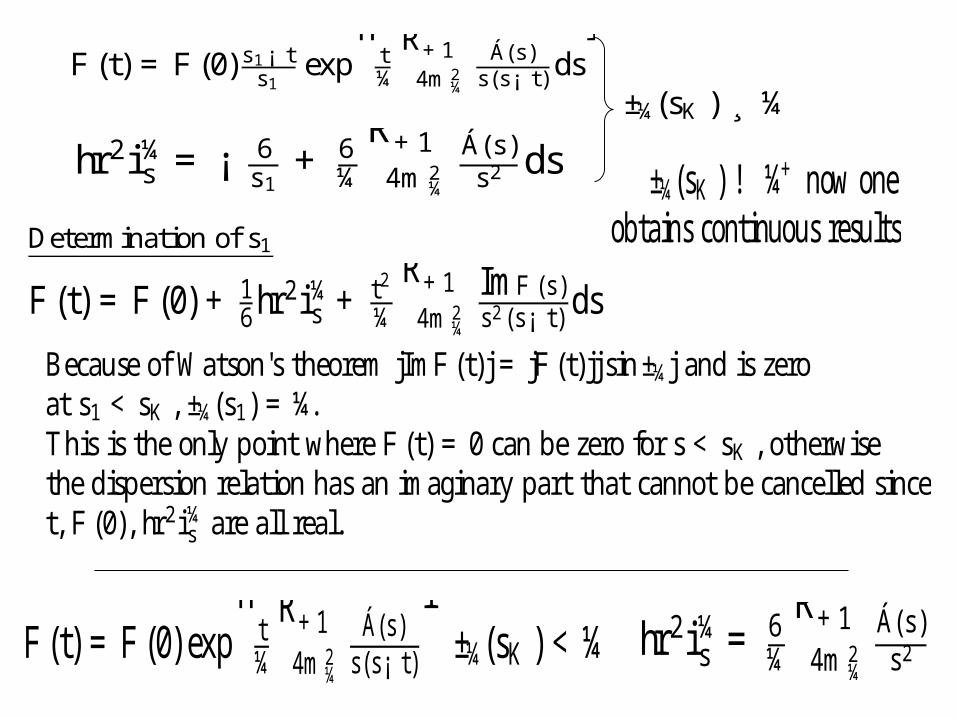
F (t) = F (0) expht¼

R+14m2

¼

Á(s)s(s¡ t)

i±¼(sK ) <¼

±¼(sK ) ¸ ¼

hr2i¼s =6¼

R+14m2

¼

Á(s)s2

±¼(sK ) ! ¼+ now oneobtains continuous results

Becauseof Watson's theorem jImF (t)j = jF (t)jj sin±¼j and is zeroat s1 < sK , ±¼(s1) =¼.This is theonly point where F (t) = 0 can bezero for s < sK , otherwisethedispersion relation has an imaginary part that cannot becancelled sincet, F (0), hr2i¼s areall real.

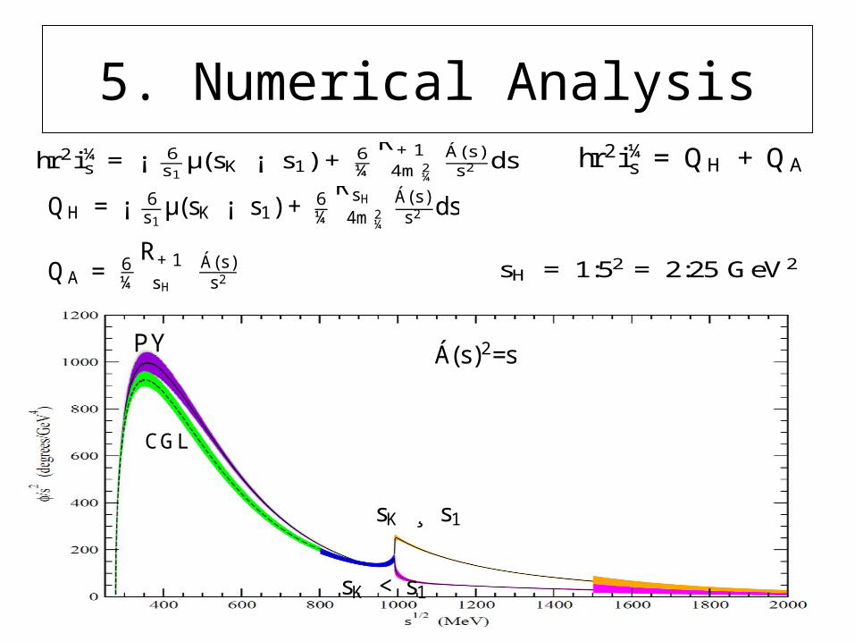
5. Numerical Analysis

QH = ¡ 6s1µ(sK ¡ s1) + 6

¼

RsH4m2

¼

Á(s)s2 ds

QA = 6¼

R+1sH

Á(s)s2

hr2i¼s = ¡ 6s1µ(sK ¡ s1) + 6

¼

R+14m2

¼

Á(s)s2 ds hr2i¼s =QH +QA

sH =1:52 =2:25GeV2

Á(s)2=s

sK ¸ s1

sK < s1

CGL

PY

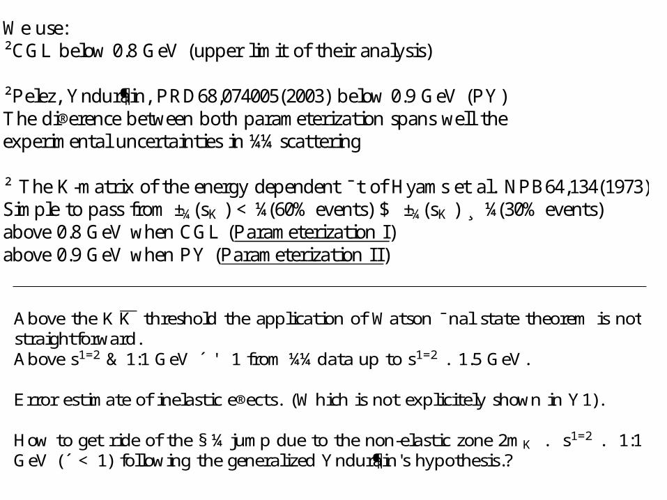
Weuse:²CGL below 0.8GeV (upper limit of their analysis)

²Pelez, Yndur¶ain, PRD68,074005(2003) below 0.9GeV (PY)Thedi®erencebetween both parameterization spans well theexperimental uncertainties in ¼¼scattering

² TheK-matrix of theenergy dependent ¯t of Hyams et al. NPB64,134(1973)Simple to pass from±¼(sK ) <¼(60%events) $ ±¼(sK ) ¸ ¼(30%events)above0.8GeV when CGL (Parameterization I)above0.9GeV when PY (Parameterization II)

Above the K K threshold the application of Watson ¯nal state theorem is notstraightforward.Aboves1=2 & 1:1 GeV ´ ' 1 from¼¼data up to s1=2 . 1.5GeV.

Error estimateof inelastic e®ects. (Which is not explicitely shown in Y1).

How to get ride of the § ¼jump due to thenon-elastic zone2mK . s1=2 . 1:1GeV (´ < 1) following thegeneralized Yndur¶ain's hypothesis.?

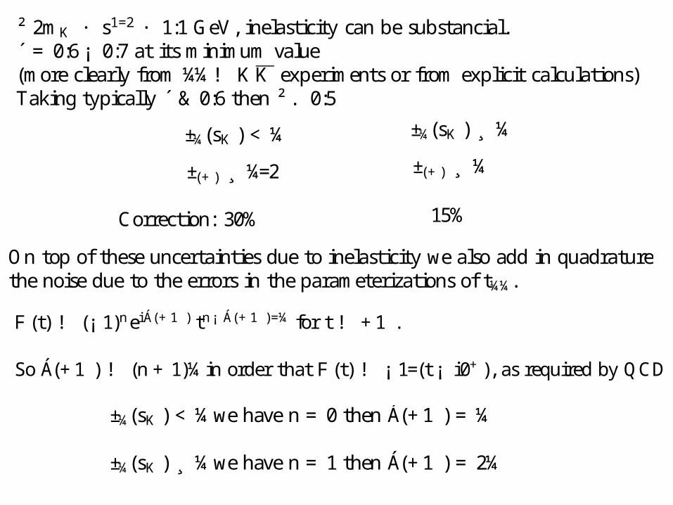
² 2mK · s1=2 · 1:1 GeV, inelasticity can besubstancial.´ = 0:6¡ 0:7 at itsminimumvalue(moreclearly from¼¼! K K experiments or fromexplicit calculations)Taking typically ´ & 0:6 then ² . 0:5

±¼(sK ) <¼ ±¼(sK ) ¸ ¼

Correction: 30%

±(+) ¸ ¼

15%

±(+) ¸ ¼=2

On top of theseuncertainties due to inelasticity wealso add in quadraturethenoisedue to theerrors in theparameterizations of t¼¼.

F (t) ! (¡ 1)neiÁ(+1 ) tn¡ Á(+1 )=¼ for t ! +1 .

So Á(+1 ) ! (n+1)¼in order that F (t) ! ¡ 1=(t ¡ i0+), as required by QCD

±¼(sK ) <¼wehaven = 0 then Á(+1 ) =¼

±¼(sK ) ¸ ¼wehaven = 1 then Á(+1 ) = 2¼

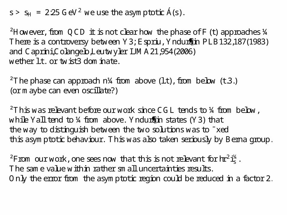
s > sH =2:25GeV2 weuse theasymptotic Á(s).

²However, fromQCD it is not clear how thephaseof F (t) approaches¼There is a controversy between Y3; Espriu, Yndur¶ain PLB132,187(1983)and Caprini,Colangelo,Leutwyler IJ MA21,954(2006)wether l.t. or twist3 dominate.

²Thephasecan approach n¼fromabove (l.t), frombelow (t.3.)(or maybecan even oscillate?)

²This was relevant beforeour work sinceCGL tends to¼frombelow,while Yall tend to¼fromabove. Yndur¶ain states (Y3) thattheway to distinguish between the two solutions was to ¯xedthis asymptotic behaviour. This was also taken seriously by Berna group.

²Fromour work, onesees now that this is not relevant for hr2i¼s .The samevaluewithin rather small uncertainties results.Only theerror from theasymptotic region could be reduced in a factor 2.

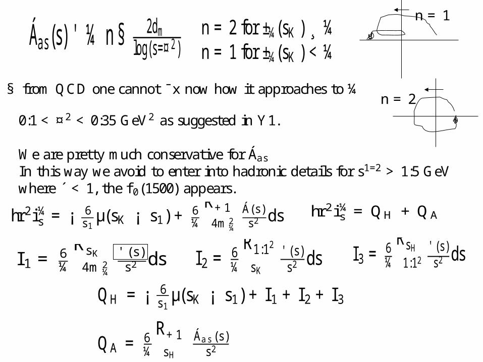
Áas(s) ' ¼³n § 2dm

log(s=¤ 2)

´n = 2 for ±¼(sK ) ¸ ¼n = 1 for ±¼(sK ) <¼

0:1< ¤2 <0:35GeV2 as suggested in Y1.

Wearepretty much conservative for ÁasIn this way weavoid to enter into hadronic details for s1=2 >1:5GeVwhere ´ < 1, the f 0(1500) appears.

hr2i¼s = ¡ 6s1µ(sK ¡ s1) + 6

¼

R+14m2

¼

Á(s)s2 ds

hr2i¼s =QH +QA

I 2 = 6¼

R1:12sK

' (s)s2 ds I 3 = 6

¼

RsH1:12

' (s)s2 dsI 1 = 6

¼

RsK4m2

¼

' (s)s2 ds

QH = ¡ 6s1µ(sK ¡ s1) + I 1+I 2+I 3

QA = 6¼

R+1sH

Áas (s)s2

§ fromQCD onecannot ¯x now how it approaches to¼

n = 1

n = 2

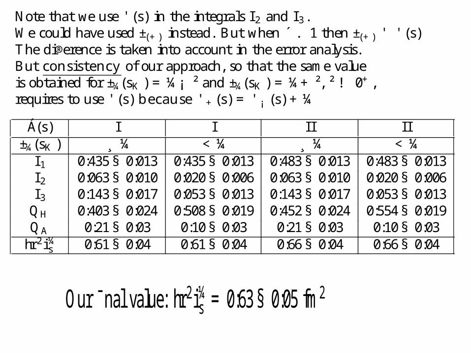
Note that weuse ' (s) in the integrals I 2 and I 3.Wecould haveused ±(+) instead. But when ´ . 1 then ±(+) ' ' (s)Thedi®erence is taken into account in theerror analysis.But consistency of our approach, so that thesamevalueis obtained for ±¼(sK ) =¼¡ ² and ±¼(sK ) =¼+², ² ! 0+,requires to use ' (s) because ' +(s) = ' ¡ (s) +¼

Á(s) I I I I I I±¼(sK ) ¸ ¼ <¼ ¸ ¼ <¼I 1 0:435§ 0:013 0:435§ 0:013 0:483§ 0:013 0:483§ 0:013I 2 0:063§ 0:010 0:020§ 0:006 0:063§ 0:010 0:020§ 0:006I 3 0:143§ 0:017 0:053§ 0:013 0:143§ 0:017 0:053§ 0:013QH 0:403§ 0:024 0:508§ 0:019 0:452§ 0:024 0:554§ 0:019QA 0:21§ 0:03 0:10§ 0:03 0:21§ 0:03 0:10§ 0:03hr2i¼s 0:61§ 0:04 0:61§ 0:04 0:66§ 0:04 0:66§ 0:04

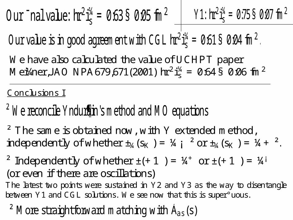
Our ¯nal value: hr2i¼s =0:63§ 0:05 fm2

The latest two points were sustained in Y2 and Y3 as the way to disentanglebetween Y1 and CGL solutions. We see now that this is super°uous.

Our value is in good agreement with CGL hr2i¼s =0:61§ 0:04 fm2.

Our ¯nal value: hr2i¼s =0:63§ 0:05 fm2

² We reconcileYndur¶ain'smethod and MO equationsConclusions I

² Thesame is obtained now, with Y extended method,independently of whether ±¼(sK ) =¼¡ ² or ±¼(sK ) =¼+².

Y1: hr2i¼s = 0:75§ 0:07 fm2

² Morestraightforward matchingwith Áas(s)

² Independently of whether ±(+1 ) =¼+ or ±(+1 ) =¼¡

(or even if thereareoscillations)

Wehavealso calculated thevalueof UCHPT paperMei¼ner,J AO NPA679,671(2001) hr2i¼s =0:64§ 0:06 fm2

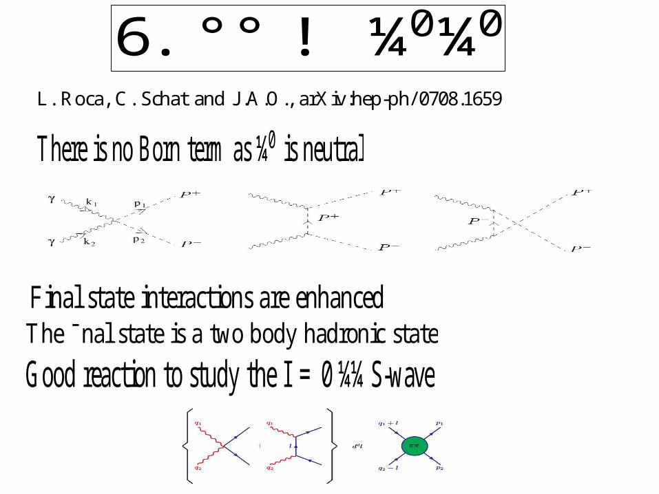
6. °° ! ¼0¼0

There is no Born termas¼0 is neutral

Final state interactions areenhancedThe¯nal state is a two body hadronic state

Good reaction to study the I = 0¼¼S-wave

L. Roca, C. Schat and J .A.O., arXiv:hep-ph/ 0708.1659

² OneloopÂPT istheleadingcontribution: Bijnens, Cornet NPB296,557(1988);PRD37,2423(1988)

² Nocounterterms, pureÂPT quantumprediction (theagreement with datawas not satisfactory)

² Two loop calculation in ÂPT was performed: Bellucci, Gasser, SainioNPB423,80 (1994), revised in Gasser,Ivanov, Sainio NPB728,31 (2005).

² Better agreement with data. Thethreecountertermswere¯xed accordingto the resonance saturation hypothesis.

Silver mode for ÂP T

¾(°° ! ¼0¼0) wasmeasured for j cosµj < 0:8by Crystal Ball Collaboration, H.Marsiskeet al. PRD41,3324 (1990)

New accuratedata on °° ! ¼+¼¡ j cosµj < 0:6T. Mori et al. [BelleColl.] PRD75,051101 (2007)Remarkable resolution of the f 0(980) resonance.

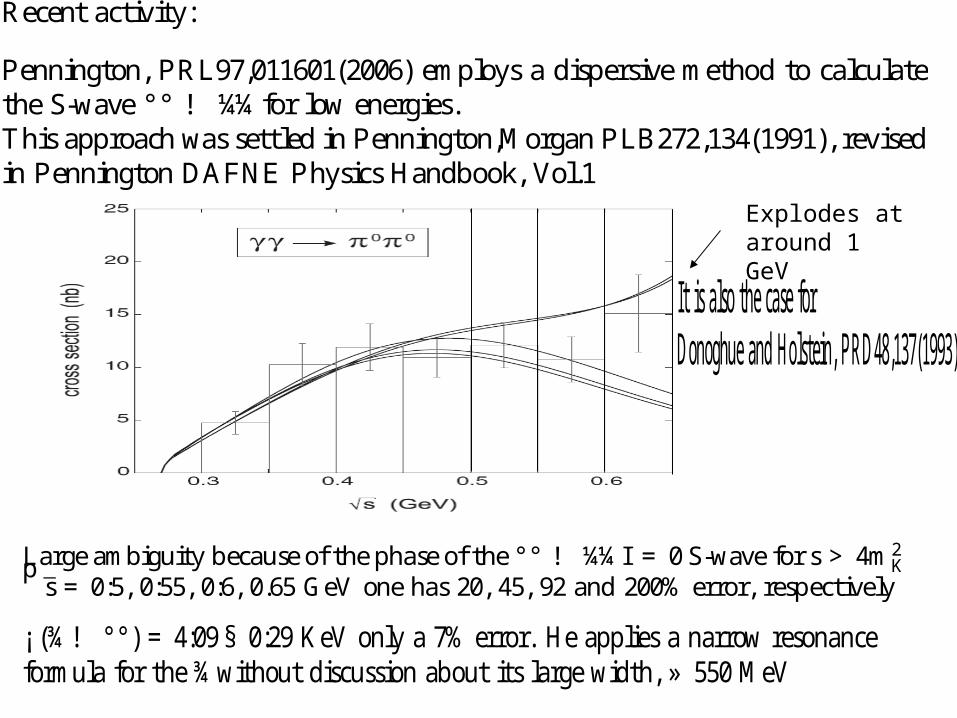
Recent activity:

Pennington, PRL97,011601(2006) employs a dispersivemethod to calculatetheS-wave°° ! ¼¼for low energies.Thisapproachwassettled in Pennington,MorganPLB272,134(1991), revisedin Pennington DAFNE Physics Handbook, Vol.1

Explodes at around 1 GeV

It is also thecase forDonoghueand Holstein, PRD48,137(1993)

Largeambiguity becauseof thephaseof the°° ! ¼¼I = 0S-wavefor s > 4m2Kp

s = 0:5, 0:55, 0:6, 0.65GeV onehas 20, 45, 92 and 200% error, respectively

¡ (¾! °°) = 4:09§ 0:29 KeV only a 7% error. Heapplies a narrow resonanceformula for the¾without discussion about its largewidth, » 550MeV

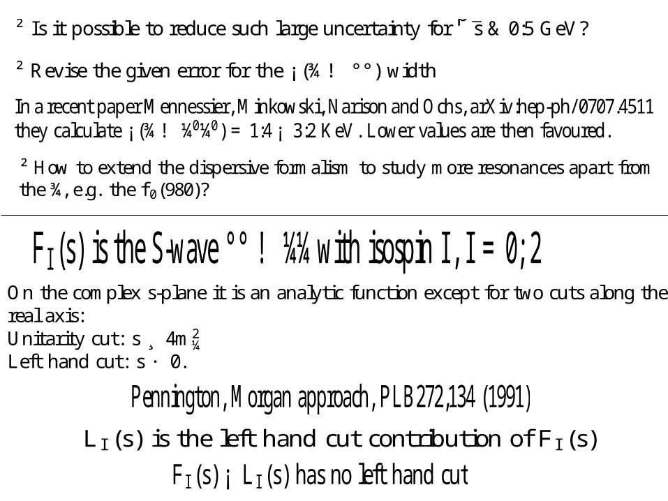
² Is it possible to reduce such largeuncertainty forps & 0:5 GeV?

Inarecent paper Mennessier, Minkowski, NarisonandOchs, arXiv:hep-ph/0707.4511they calculate ¡ (¾! ¼0¼0) = 1:4¡ 3:2 KeV. Lower values are then favoured.

² Revise thegiven error for the ¡ (¾! °°) width

² How to extend thedispersive formalism to study moreresonances apart fromthe¾, e.g. the f 0(980)?

F I (s) is theS-wave °° ! ¼¼with isospin I , I = 0; 2

L I (s) is the left hand cut contribution of F I (s)

F I (s) ¡ L I (s) has no left hand cut

On thecomplex s-plane it is an analytic function except for two cuts along thereal axis:Unitarity cut: s ¸ 4m2

¼Left hand cut: s · 0.

Pennington, Morgan approach, PLB272,134 (1991)

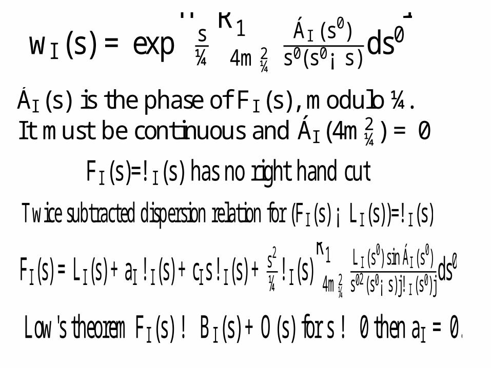
wI (s) = exphs¼

R14m2

¼

ÁI (s0)s0(s0¡ s)ds

0i

ÁI (s) is thephaseof F I (s), modulo¼.It must becontinuous and ÁI (4m2

¼) = 0

F I (s)=! I (s) has no right hand cut

Twicesubtracted dispersion relation for (F I (s) ¡ L I (s))=! I (s)

F I (s) = L I (s) +aI ! I (s) +cI s! I (s) + s2

¼! I (s)R14m2

¼

L I (s0) sin ÁI (s

0)s02(s0¡ s)j! I (s0)j

ds0

Low's theoremF I (s) ! B I (s) +O(s) for s ! 0 then aI =0.

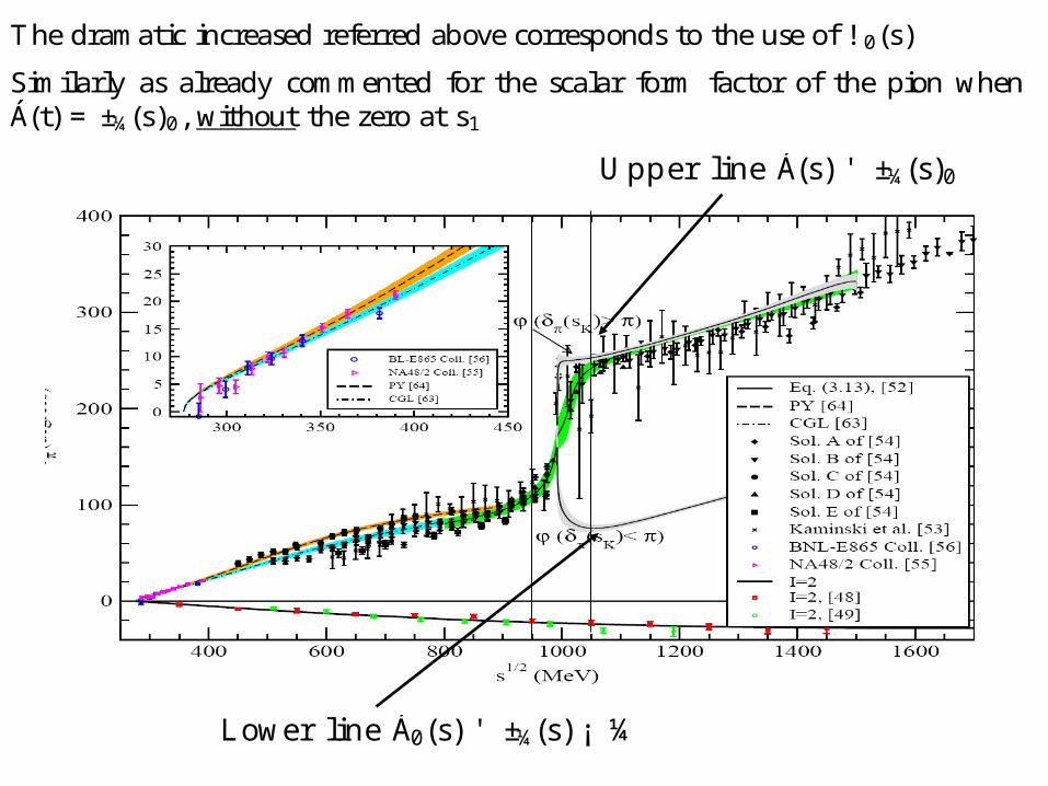
Lower line Á0(s) ' ±¼(s) ¡ ¼

Upper line Á(s) ' ±¼(s)0

Thedramatic increased referred abovecorresponds to theuseof ! 0(s)

Similarly as already commented for the scalar form factor of the pion whenÁ(t) =±¼(s)0, without the zero at s1

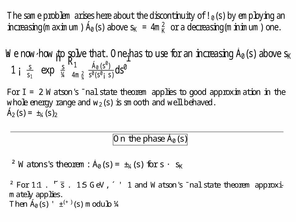
Thesameproblemarises hereabout thediscontinuity of ! 0(s) by employinganincreasing(maximum) Á0(s) abovesK =4m2

K or a decreasing(minimum) one.

For I = 2 Watson's ¯nal state theorem applies to good approximation in thewholeenergy rangeand w2(s) is smooth and well behaved.Á2(s) =±¼(s)2

On thephaseÁ0(s)

² Watons's theorem: Á0(s) = ±¼(s) for s · sK

² For 1:1 .ps . 1:5 GeV, ´ ' 1 and Watson's ¯nal state theorem approxi-

mately applies.Then Á0(s) ' ±(+)(s) modulo ¼

Wenow how to solve that. Onehas to use for an increasing Á0(s) abovesK :³1¡ s

s1

´exp

hs¼

R14m2

¼

Á0(s0)s0(s0¡ s)ds

0i

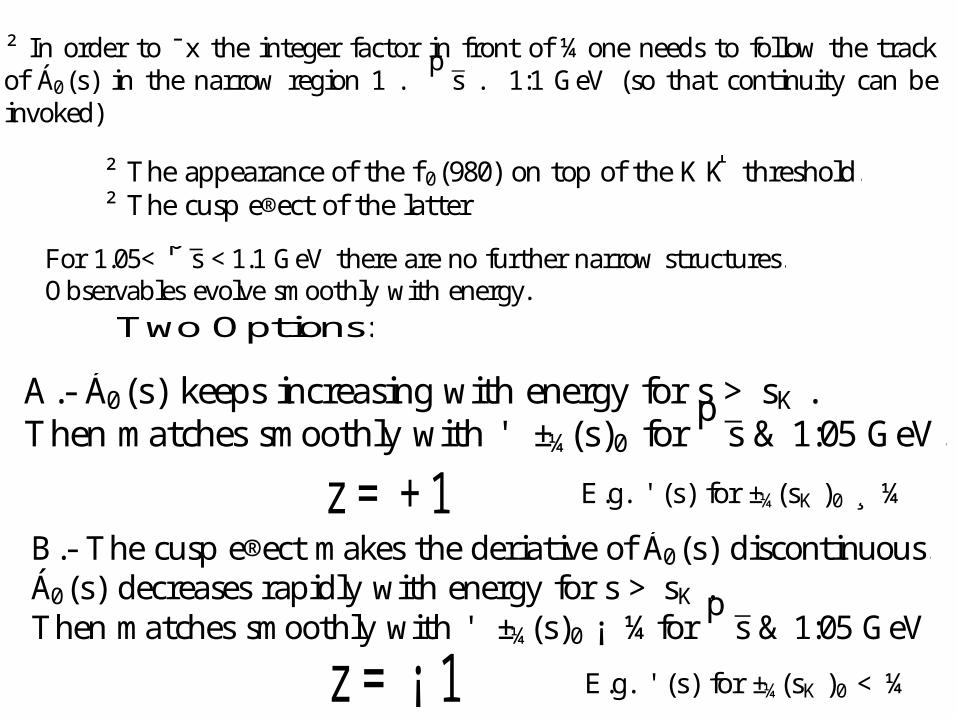
² In order to ¯x the integer factor in front of ¼one needs to follow the trackof Á0(s) in the narrow region 1 .

ps . 1:1 GeV (so that continuity can be

invoked)

For 1.05<ps <1.1 GeV thereareno further narrow structures.

Observables evolve smoothly with energy.Two Options:

z =+1

z = ¡ 1

E.g. ' (s) for ±¼(sK )0 ¸ ¼

E.g. ' (s) for ±¼(sK )0 <¼

² Theappearanceof the f 0(980) on top of theK ¹K threshold.² Thecusp e®ect of the latter

A.- Á0(s) keeps increasingwith energy for s > sK .Then matches smoothly with ' ±¼(s)0 for

ps & 1:05GeV.

B.- Thecusp e®ect makes thederiativeof Á0(s) discontinuous.Á0(s) decreases rapidly with energy for s > sK .Then matches smoothly with ' ±¼(s)0 ¡ ¼for

ps & 1:05GeV

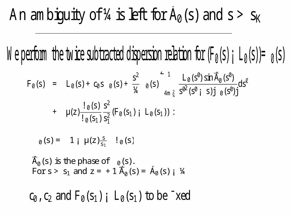
Weperform the twice subtracted dispersion relation for (F0(s) ¡ L0(s))=­ 0(s)F0(s) = L0(s) +c0s­ 0(s) +

s2

¼­ 0(s)

Z 1

4m2¼

L0(s0) sinÁ0(s0)

s02(s0¡ s)j­ 0(s0)jds0

+ µ(z)! 0(s)! 0(s1)

s2

s21(F0(s1) ¡ L0(s1)) :

­ 0(s) =³1¡ µ(z) ss1

´! 0(s)

Á0(s) is thephaseof ­ 0(s).For s > s1 and z =+1Á0(s) = Á0(s) ¡ ¼

An ambiguity of ¼is left for Á0(s) and s > sK

c0, c2 and F0(s1) ¡ L0(s1) to be ¯xed

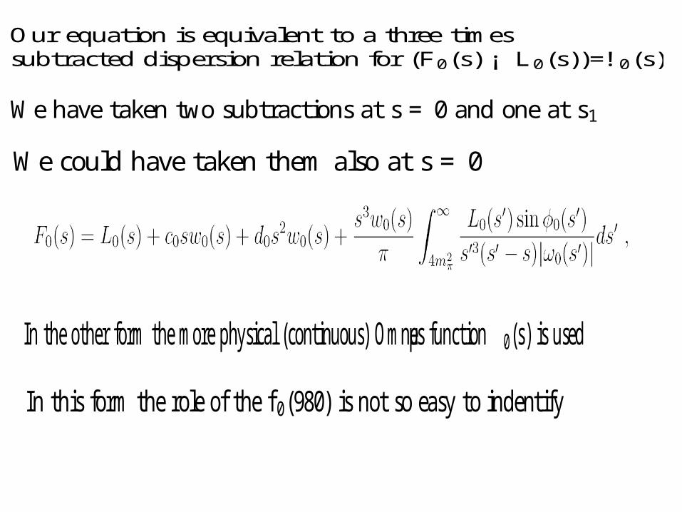
Our equation is equivalent to a three timessubtracted dispersion relation for (F0(s) ¡ L0(s))=! 0(s)

Wehave taken two subtractions at s = 0 and oneat s1

Wecould have taken themalso at s = 0

In this form the roleof the f 0(980) is not so easy to indentify

In theother form themorephysical (continuous) Omnµes function ­ 0(s) is used

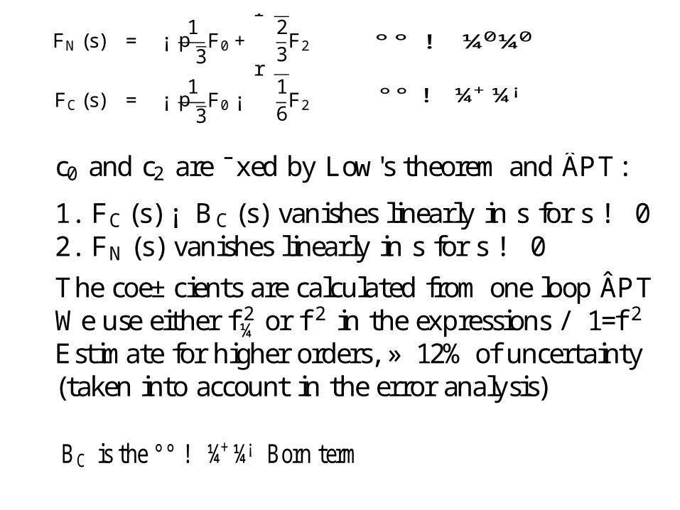
FN (s) = ¡1p3F0+

r23F2

FC (s) = ¡1p3F0 ¡

r16F2 °° ! ¼+¼¡

°° ! ¼0¼0

c0 and c2 are ¯xed by Low's theoremand ÂPT:

1. FC (s) ¡ BC (s) vanishes linearly in s for s ! 02. FN (s) vanishes linearly in s for s ! 0

Thecoe±cients arecalculated fromone loop ÂPTWeuseeither f 2¼ or f

2 in theexpressions / 1=f 2

Estimate for higher orders, » 12% of uncertainty(taken into account in theerror analysis)

BC is the °° ! ¼+¼¡ Born term

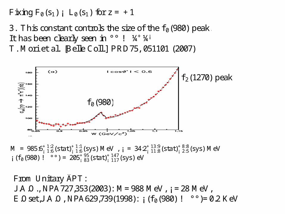
Fixing F0(s1) ¡ L0(s1) for z =+1

f 2(1270) peak

f 0(980)

FromUnitary ÂPT:J .A.O., NPA727,353(2003): M=988MeV, ¡ =28MeV,E.Oset,J .A.O, NPA629,739(1998): ¡ (f 0(980) ! °°)=0.2 KeV

3. This constant controls thesizeof the f 0(980) peak.It has been clearly seen in °° ! ¼+¼¡

T. Mori et al. [BelleColl.] PRD75, 051101 (2007)

M =985:6+1:2¡ 1:6(stat)+1:1¡ 1:6(sys) MeV , ¡ = 34:2+13:9¡ 11:8(stat)

+8:8¡ 2:5(sys) MeV

¡ (f 0(980) ! °°) = 205+95¡ 83(stat)+147¡ 117(sys) eV

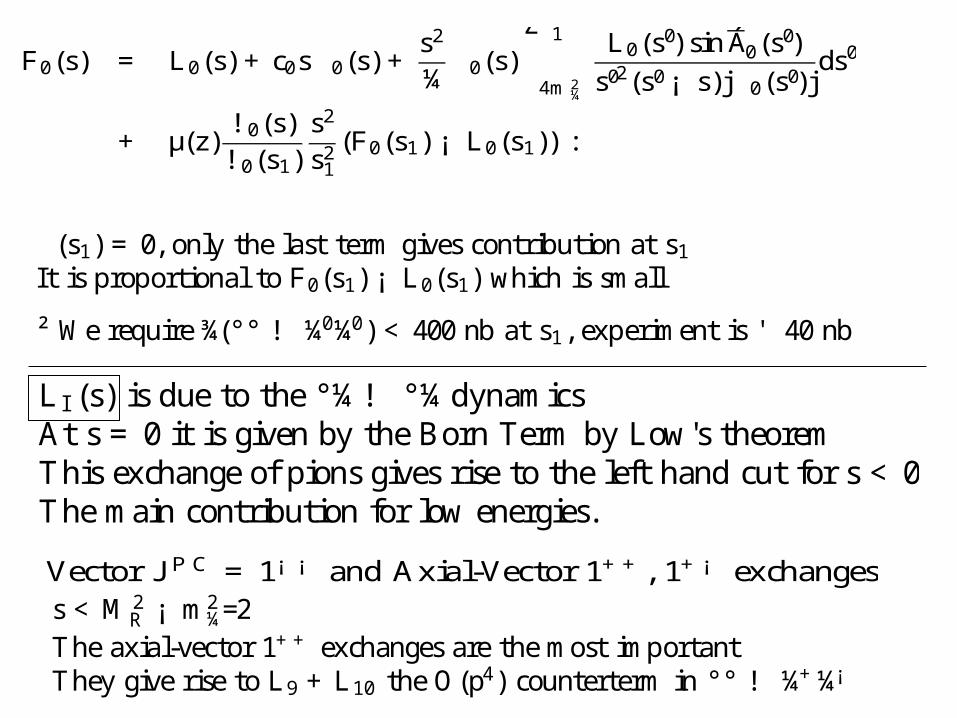
F0(s) = L0(s) +c0s­ 0(s) +s2

¼­ 0(s)

Z 1

4m2¼

L0(s0) sinÁ0(s0)

s02(s0¡ s)j­ 0(s0)jds0

+ µ(z)! 0(s)! 0(s1)

s2

s21(F0(s1) ¡ L0(s1)) :

­ (s1) = 0, only the last termgives contribution at s1It is proportional to F0(s1) ¡ L0(s1) which is small

L I (s) is due to the °¼! °¼dynamicsAt s = 0 it is given by theBorn Termby Low's theoremThis exchangeof pions gives rise to the left hand cut for s < 0Themain contribution for low energies.

Vector J P C =1¡ ¡ and Axial-Vector 1++, 1+¡ exchanges

² We require¾(°° ! ¼0¼0) < 400 nb at s1, experiment is ' 40 nb

Theaxial-vector 1++ exchanges are themost importantThey give rise to L9+L10 theO(p4) counterterm in °° ! ¼+¼¡

s <M 2R ¡ m2

¼=2

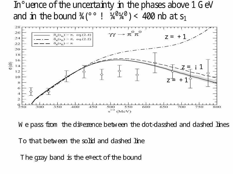
In°uenceof theuncertainty in thephases above1GeVand in thebound ¾(°° ! ¼0¼0) < 400 nb at s1

Wepass from thedi®erencebetween thedot-dasshed and dashed lines

To that between thesolid and dashed line

z =+1

z =+1

z = ¡ 1

Thegray band is thee®ect of thebound

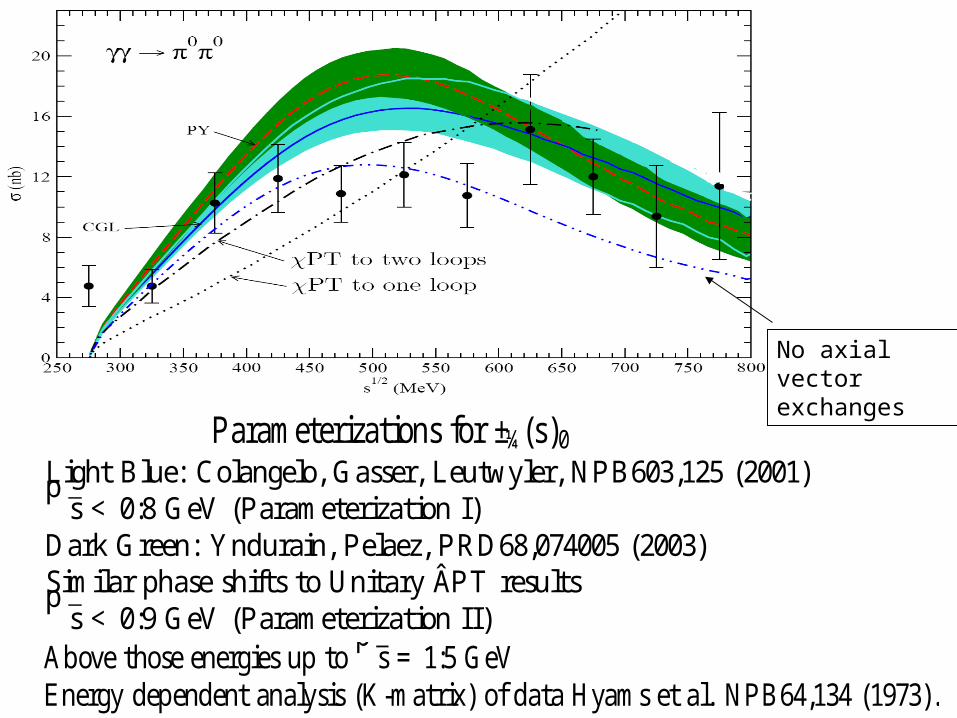
Parameterizations for ±¼(s)0

Above thoseenergies up tops = 1:5GeV

Energy dependent analysis (K-matrix) of data Hyams et al. NPB64,134 (1973).

Light Blue: Colangelo, Gasser, Leutwyler, NPB603,125 (2001)ps < 0:8 GeV (Parameterization I)

Dark Green: Yndurain, Pelaez, PRD68,074005 (2003)Similar phase shifts to Unitary ÂPT resultsps < 0:9 GeV (Parameterization II)

No axial vector exchanges

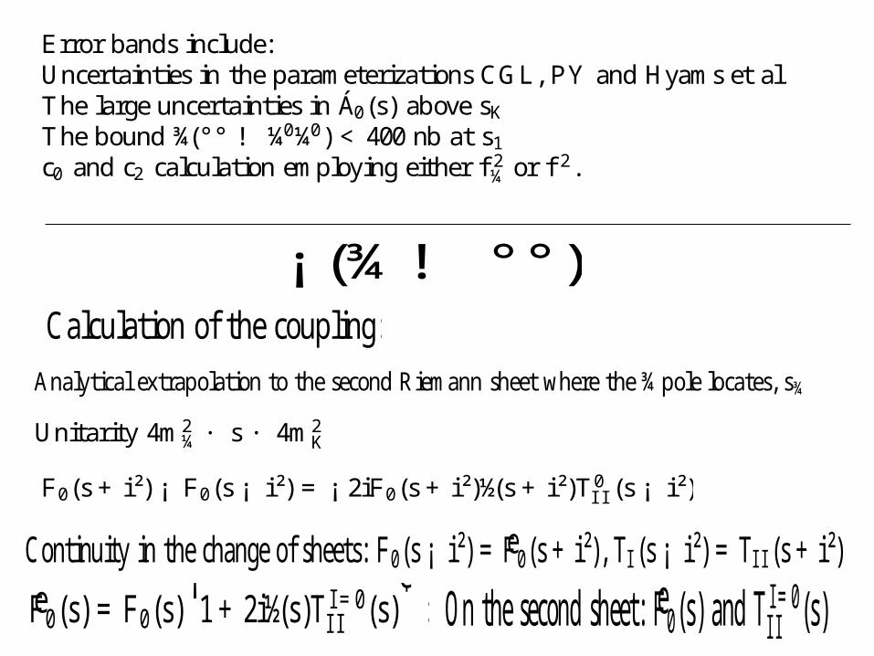
Error bands include:Uncertainties in theparameterizations CGL, PY and Hyams et al.The largeuncertainties in Á0(s) abovesKThebound ¾(°° ! ¼0¼0) < 400 nb at s1c0 and c2 calculation employing either f 2¼ or f

2.

¡ (¾! °°)Calculation of thecoupling:Analytical extrapolation to thesecond Riemann sheet where the¾pole locates, s¾

Unitarity 4m2¼ · s · 4m2

K

F0(s+ i²) ¡ F0(s ¡ i²) = ¡ 2iF0(s+ i²)½(s+ i²)T0I I (s ¡ i²)

eF0(s) = F0(s)¡1+2i½(s)T I =0

I I (s)¢:

Continuity in thechangeof sheets: F0(s ¡ i²) = eF0(s+ i²), TI (s ¡ i²) = TI I (s+ i²)

On thesecond sheet: eF0(s) and T I =0I I (s)

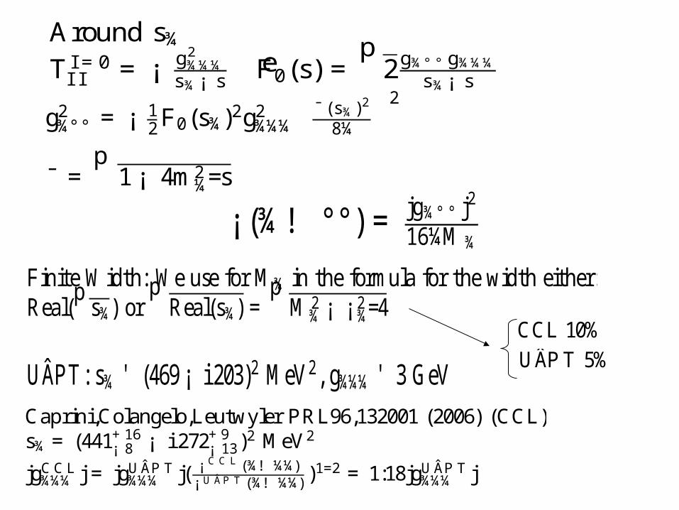
Around s¾T I =0I I = ¡ g2¾¼¼

s¾¡ seF0(s) =

p2g¾° ° g¾¼¼s¾¡ s

g2¾°° = ¡ 12F0(s¾)

2g2¾¼¼³¯ (s¾)2

8¼

´2

¯ =p1¡ 4m2

¼=s

¡ (¾! °°) = jg¾° ° j2

16¼M ¾

FiniteWidth: Weuse for M¾ in the formula for thewidth either:Real(

ps¾) or

pReal(s¾) =

pM 2

¾¡ ¡ 2¾=4

UÂPT: s¾ ' (469¡ i 203)2 MeV2, g¾¼¼ ' 3 GeVUÂPT 5%CCL 10%

Caprini,Colangelo,Leutwyler PRL96,132001 (2006) (CCL)s¾= (441+16¡ 8 ¡ i 272+9¡ 13)

2 MeV2

jgCCL¾¼¼ j = jgUÂP T¾¼¼ j( ¡ C C L (¾! ¼¼)¡ U ÂP T (¾! ¼¼) )

1=2 =1:18jgUÂP T¾¼¼ j

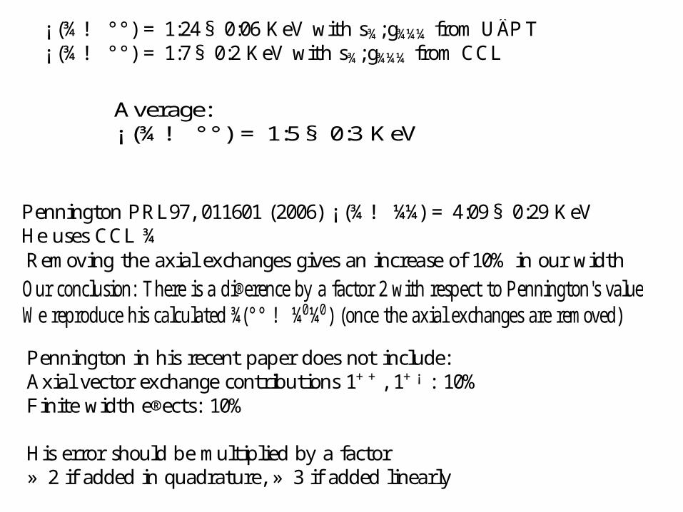
¡ (¾! °°) = 1:24§ 0:06 KeV with s¾;g¾¼¼ fromUÂPT¡ (¾! °°) = 1:7§ 0:2 KeV with s¾;g¾¼¼ fromCCL

Average:¡ (¾! °°) = 1:5§ 0:3 KeV

Removing theaxial exchanges gives an increaseof 10% in our width

Pennington PRL97, 011601 (2006) ¡ (¾! ¼¼) = 4:09§ 0:29 KeVHeuses CCL ¾

Our conclusion: There is a di®erenceby a factor 2with respect to Pennington's valueWereproducehis calculated ¾(°° ! ¼0¼0) (once theaxial exchanges are removed)

Pennington in his recent paper does not include:Axial vector exchangecontributions 1++, 1+¡ : 10%Finitewidth e®ects: 10%

His error should bemultiplied by a factor» 2 if added in quadrature, » 3 if added linearly

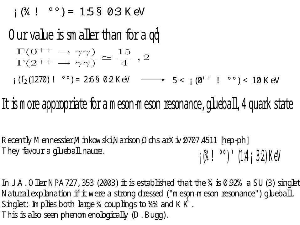
Our value is smaller than for a q¹q

¡ (f 2(1270) ! °°) = 2:6§ 0:2 KeV 5< ¡ (0++ ! °°) < 10KeV

¡ (¾! °°) = 1:5§ 0:3 KeV

It is moreappropriate for ameson-meson resonance, glueball, 4 quark state

¡ (¾! °°) ' (1:4¡ 3:2) KeVRecently Mennessier,Minkowski,Narison,Ochs arXiv:0707.4511 [hep-ph]They favour a glueball naure.

In J .A. Oller NPA727, 353 (2003) it is established that the¾is 0.92% a SU(3) singletNatural explanation if it werea strong dressed ("meson-meson resonance") glueball.Singlet: Implies both large¾couplings to¼¼and K ¹K .This is also seen phenomenologically (D. Bugg).

7. Conclusions II

² Onecan discern among di®erent I = 0 S-wave¼¼parameterizationswhen new and moreprecisedata becomeavailable.

² ¡ (¾! ¼¼) = 1:5§ 0:3 KeVNon q¹q resonance.

² Themethod is also adequate to study the f 0(980) resonance.L. Roca, C. Schat and J .A.O. , to appear soon.

² Wehavehandled with three subtractions constants (moreprecisision)instead of the two used previously in the literature.

² Drastic reduction in theuncertainty of ¾(°° ! ¼0¼0) forps & 0:5GeV

due to theuncertainty in Á0(s) abovesK .

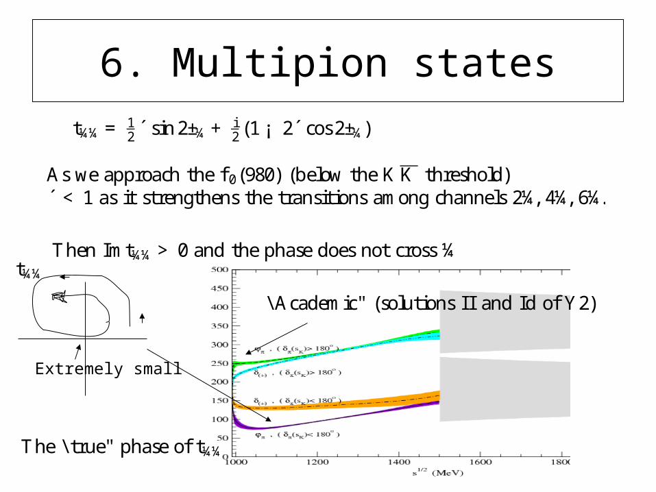
6. Multipion states

t¼¼= 12´ sin2±¼+

i2(1¡ 2́ cos2±¼)

Then Imt¼¼> 0and thephasedoes not cross¼

Extremely small

t¼¼

The \ true" phaseof t¼¼

\ Academic" (solutions II and Id of Y2)

Asweapproach the f 0(980) (below theK K threshold)´ < 1 as it strengthens the transitions among channels 2¼, 4¼, 6¼.

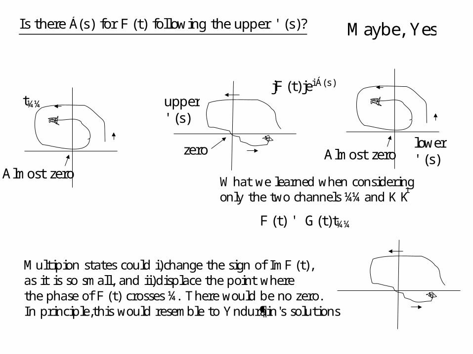
Is thereÁ(s) for F (t) following theupper ' (s)?

jF (t)jeiÁ(s)t¼¼

Almost zero

F (t) ' G(t)t¼¼

Almost zero

upper' (s)

lower' (s)

Maybe, Yes

zero

What we learned when consideringonly the two channels¼¼and K ¹K

Multipion states could i)change thesign of ImF (t),as it is so small, and ii)displace thepoint wherethephaseof F (t) crosses¼. Therewould beno zero.In principle,this would resemble to Yndur¶ain's solutions

Note that ImF (t) can changesignThis is not thecase for t¼¼ becauseof unitarityImt¼¼ ¸ 0

However, F (t) would then develop almost a pole (strongmaximum)and then wepass to an unacceptable situation from thepoint of view of thestarting hypothesis of theperturbativee®ect of multipion states.

This is remedied if one introduces a zero at s1 and then,onecomes back again to theOR solution with a zero.

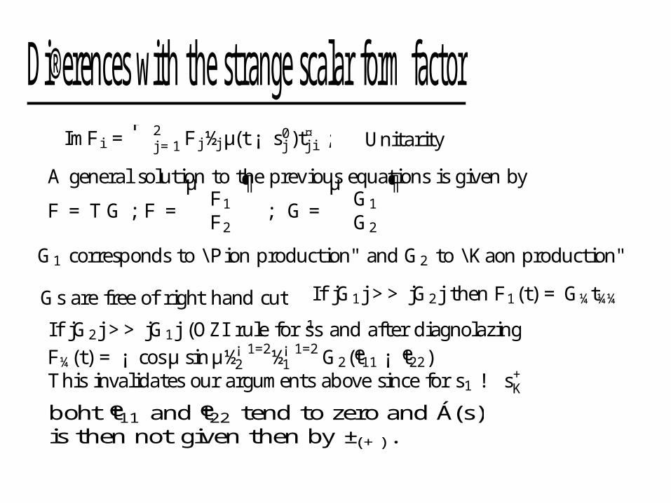
Di®erenceswith thestrangescalar form factorImF i =

P 2j =1F j½j µ(t ¡ s0j )t

¤j i ; Unitarity

A general solution to theprevious equations is given by

F = T G ; F =µF1F2

¶; G =

µG1

G2

¶

G1 corresponds to \ Pion production" and G2 to \Kaon production"

Gs are freeof right hand cut If jG1j >> jG2j then F1(t) = G¼t¼¼

If jG2j >> jG1j (OZI rule for ¹ss and after diagnolazingF¼(t) = ¡ cosµ sinµ½¡ 1=22 ½¡ 1=21 G2(et11 ¡ et22)This invalidates our arguments abovesince for s1 ! s+Kboht et11 and et22 tend to zero and Á(s)is then not given then by ±(+).

Also for jG2j >> jG1j then j¡ 02=¡01j ' jet11 tanµ=et22j

For typical values jet11=et22j ' 1 thenj¡ 02=¡

01j ' j tanµj < 1

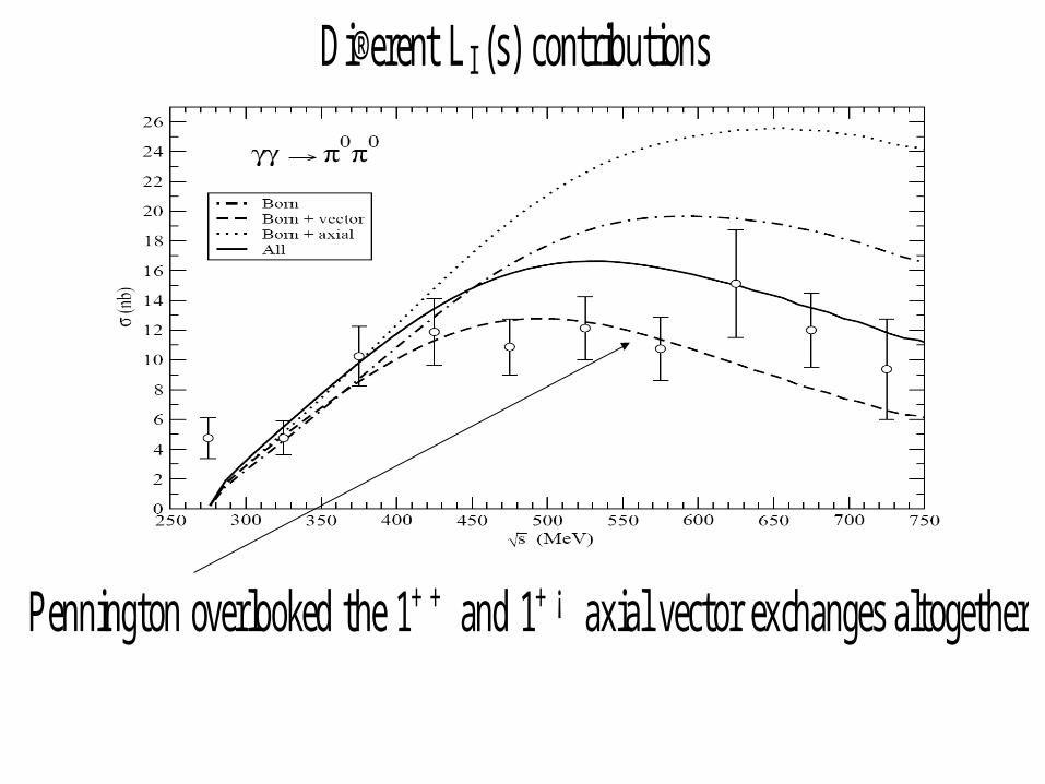
Di®erent L I (s) contributions

Pennington overlooked the1++ and 1+¡ axial vector exchanges altogether

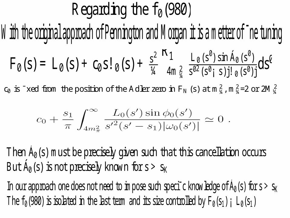
Regarding the f 0(980)

c0 is ¯xed from theposition of theAdler zero in FN (s) at m2¼, m

2¼=2or 2M

2¼

Then Á0(s) must beprecisely given such that this cancellation occursBut Á0(s) is not precisely known for s > sK

With theoriginal approach of Pennington and Morgan it is ametter of ¯ne tuning

F0(s) = L0(s) +c0s! 0(s) + s2

¼

R14m2

¼

L 0(s0) sin Á0(s

0)s02(s0¡ s)j! 0(s0)j

ds0

In our approach onedoes not need to impose such speci¯c knowledgeof Á0(s) for s > sKThe f 0(980) is isolated in the last termand its size controlled by F0(s1) ¡ L0(s1)

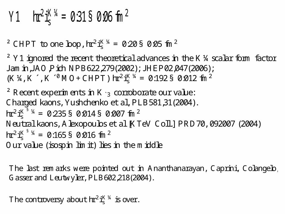
² CHPT to one loop, hr2iK ¼s =0:20§ 0:05 fm2

² Y1 ignored the recent theoretical advances in theK ¼scalar form factorJ amin,J AO,Pich NPB622,279(2002); J HEP02,047(2006);(K ¼, K ´, K ´0MO+CHPT) hr2iK ¼

s =0:192§ 0:012 fm2

² Recent experiments in K `3 corroborateour value:Charged kaons, Yushchenko et al, PLB581,31(2004).hr2iK

§ ¼s =0:235§ 0:014§ 0:007 fm2

Neutral kaons, Alexopoulos et al [KTeV Coll.] PRD70, 092007 (2004)hr2iK

§ ¼s =0:165§ 0:016 fm2

Our value (isospin limit) lies in themiddle

The last remarks were pointed out in Ananthanarayan, Caprini, Colangelo,Gasser and Leutwyler, PLB602,218(2004).

Thecontroversy about hr2iK ¼s is over.

Y1 hr2iK ¼s =0:31§ 0:06 fm2

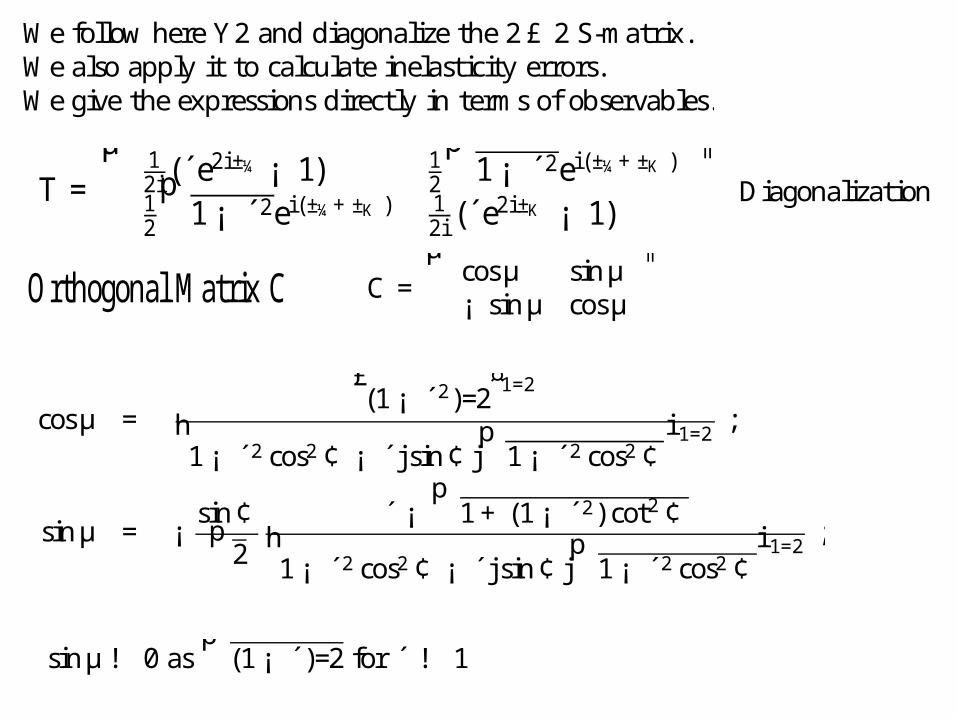
Wefollow hereY2 and diagonalize the2£ 2 S-matrix.Wealso apply it to calculate inelasticity errors.Wegive theexpressions directly in terms of observables.

T =µ

12i (´e

2i±¼ ¡ 1) 12

p1¡ ´2ei (±¼+±K )

12

p1¡ ´2ei (±¼+±K ) 1

2i (´e2i±K ¡ 1)

¶

Orthogonal Matrix C C =µcosµ sinµ¡ sinµ cosµ

¶

Diagonalization

cosµ =

£(1¡ ´2)=2

¤1=2

h1¡ ´2 cos2¢ ¡ ´j sin¢ j

p1¡ ´2 cos2¢

i 1=2 ;

sinµ = ¡sin¢p2

´ ¡p1+(1¡ ´2) cot2¢

h1¡ ´2 cos2¢ ¡ ´j sin¢ j

p1¡ ´2 cos2¢

i 1=2 ;

sinµ! 0 asp(1¡ ´)=2 for ´ ! 1

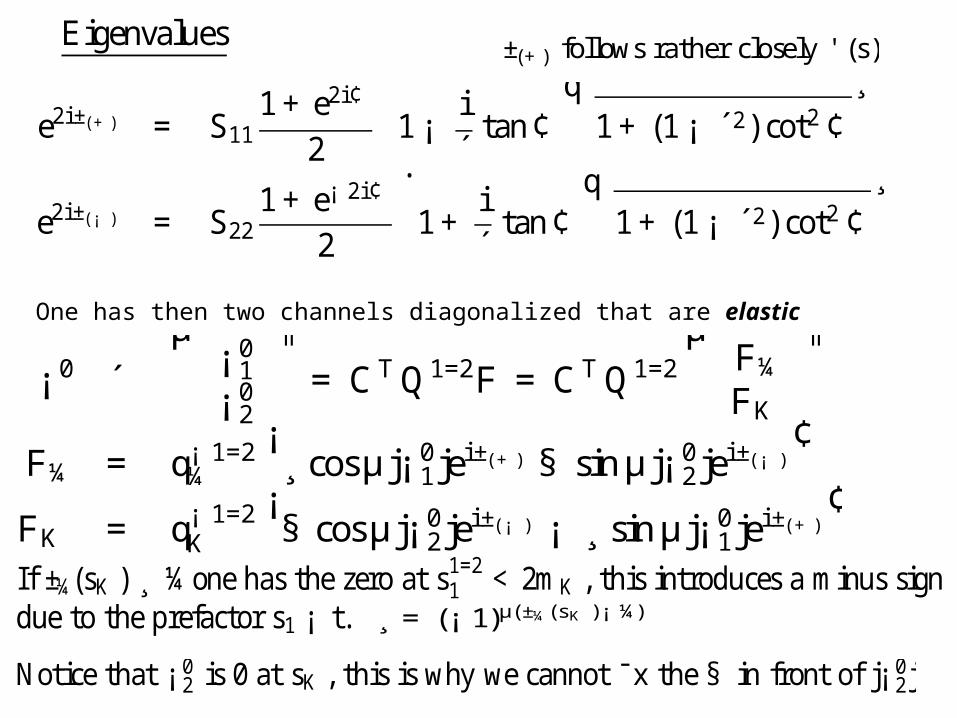
If ±¼(sK ) ¸ ¼onehas thezero at s1=21 <2mK , this introduces aminus signdue to theprefactor s1 ¡ t.

Eigenvalues

¸ = (¡ 1)µ(±¼(sK )¡ ¼)

e2i±(+ ) = S111+e2i¢

2

·1¡

i´tan¢

q1+(1¡ ´2) cot2¢

¸

e2i±( ¡ ) = S221+e¡ 2i¢

2

·1+

i´tan¢

q1+(1¡ ´2) cot2¢

¸

One has then two channels diagonalized that are elastic

Notice that ¡ 02 is 0 at sK , this is why wecannot ¯x the§ in front of j¡ 02j

¡ 0 ´µ¡ 01¡ 02

¶= CTQ1=2F = CTQ1=2

µF¼FK

¶

F¼ = q¡ 1=2¼

¡¸ cosµj¡ 01je

i±(+ ) § sinµj¡ 02jei±( ¡ )

¢

FK = q¡ 1=2K

¡§ cosµj¡ 02je

i±( ¡ ) ¡ ¸ sinµj¡ 01jei±(+ )

¢

±(+) follows rather closely ' (s)

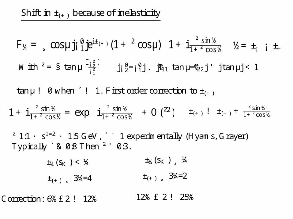
Shift in ±(+) becauseof inelasticity

F¼= ¸ cosµj¡ 01jei±(+ ) (1+² cosµ)

³1+ i ² sin½

1+² cos½

´

With ² = § tanµ¯¯¯¡

02

¡ 01

¯¯¯

tanµ! 0when ´ ! 1. First order correction to ±(+)

j¡ 02=¡01j . jet11 tanµ=et22j ' j tanµj < 1

±(+) ! ±(+) +² sin½

1+² cos½

½=±¡ ¡ ±+

1+ i ² sin½1+² cos½=exp

³i ² sin½1+² cos½

´+O(²2)

±¼(sK ) <¼

±(+) ¸ 3¼=4

Correction: 6%£2! 12%

±¼(sK ) ¸ ¼

±(+) ¸ 3¼=2

12%£ 2! 25%

² 1:1 · s1=2 · 1:5 GeV, ´ ' 1 experimentally (Hyams, Grayer).Typically ´ & 0:8 Then ² ' 0:3.

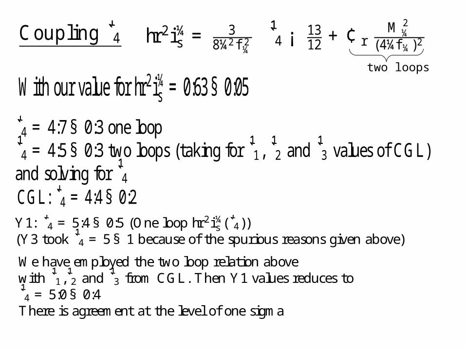
Coupling ¹̀4 hr2i¼s =

38¼2f 2¼

³¹̀4 ¡ 13

12 +¢ rM 2

¼(4¼f ¼)2

´

two loops

With our value for hr2i¼s =0:63§ 0:05¹̀4 = 4:7§ 0:3 one loop¹̀4 = 4:5§ 0:3 two loops (taking for ¹̀1, ¹̀2 and ¹̀

3 values of CGL)and solving for ¹̀4CGL: ¹̀4 =4:4§ 0:2

Wehaveemployed the two loop relation abovewith ¹̀

1,¹̀2 and ¹̀3 fromCGL. Then Y1 values reduces to

¹̀4 =5:0§ 0:4There is agreement at the level of onesigma

Y1: ¹̀4 =5:4§ 0:5 (One loop hr2i¼s (¹̀4))(Y3 took ¹̀4 =5§ 1 becauseof thespurious reasons given above)