Embed Size (px)
Citation preview
Computational and Experimental Modelling of Mooring Line
Dynamics for Offshore Floating Wind Turbines
Jose Azcona Armendariz
Ingeniero Industrial
This dissertation is submitted for the degree of:
Doctor of Philosophy
Ciencias y Tecnologıas Navales y Oceanicas
Departamento de Arquitectura, Construccion, Sistemas Oceanicos y
Navales (DACSON)
Escuela Tecnico Superior de Ingenieros Navales
Universidad Politecnica de Madrid
Defense: February 10th, 2016
(Document revision: February 9th, 2017)
Director: Dr. Leo Miguel Gonzalez Gutierrez
Co-Director: Dr. Xabier Munduate Echarri

i
Declaration
I hereby declare that except where specific reference is made to the work of others, thecontents of this dissertation are original and have not been submitted in whole or in partfor consideration for any other degree or qualification in this, or any other University. Thisdissertation is the result of my own work and includes nothing which is the outcome ofwork done in collaboration, except where specifically indicated in the text. This dissertationcontains fewer than 65,000 words including appendices, bibliography, footnotes, tables andequations and has fewer than 150 figures.
Jose Azcona ArmendarizFebruary 2016

ii
To my parents and my brother
iii
Acknowledgments
I want to acknowledge my supervisors Leo Gonzalez from the Universidad Politecnica deMadrid (UPM) and Xabier Munduate from Centro Nacional de Energıas Renovables (CENER)for their orientation and advice during my research. Leo has encouraged me in all the stepsof this research and has provided a great scientific support to this work. Xabier, who hasadvised me in my professional career since I work at CENER, greatly helped me to startthis adventure and to define the scope of the investigation.I also feel in great debt with Tor Anders Nygaard for his wise guidance in this research, forthe revision of my work and for his dedication and availability every time I needed him.Thank you to Antonio Ugarte, head of the Wind Energy Department at CENER, for hissupport during these years and for facilitating my dedication to this Ph.D. in conjunctionwith my work. Thank you also to Jorge Biera for his advice as current responsible of theAnalysis and Design of Wind Turbines service (ADA). The research in offshore wind energyrequires knowledge in many different fields of engineering. I have found a great support andavailability to solve technical doubts in all my colleagues from ADA. In particular, I have toacknowledge Joseba Garciandıa for his help with the mooring line code implementation andfor the setup of the scripts to launch the integrated simulations of floating wind turbines;Alfredo Martınez, Alvaro Gonzalez and Ainara Irisarri for assisting me in the computationof the wind turbine loads and Mikel Iribas for answering my questions relating the windturbine control. I am very grateful to Inaki Nuin, Roberto Montejo and Javier Estarriagafor our clarifying discussions on the structural models, fatigue analysis and for helping mein the meshing of the floaters for the hydrodynamic analysis. I have to recognize DavidPalacio for his collaboration on the launching and postprocessing of the simulation cases forthe analysis of the importance of mooring dynamics, and to my colleagues from the Evalua-tion and Prediction of Resource service (EPR) Elena Cantero, Pedro Miguel Fernandes andSergio Lozano for their help in the site selection for the floating wind turbine models andfor calculating the environmental wind and wave conditions for this study. Many thanks tothe colleagues with whom I have shared the office since many years ago: Beatriz Mendez,Mercedes Sanz, Ana Belen Farinas, Cristina San Bruno, Sugoi Gomez, Oscar Pires, Car-los Amezqueta, Ernesto Saenz, Marcos del Rıo, Javier San Miguel and also to all the newcolleagues that joined ADA more recently. I also have to mention Belen Arbaizar, fromCENER’s Library Service, for her great (and quick) work searching the references I needed.I have to remember Mikel Lasa, who was the responsible of the ADA service at CENER

iv
when I was starting my thesis and who supported me in my first steps, and Pablo Ayesa,who has been head of the Wind Energy Department at CENER during part of the time thatI have been working on my Ph.D. Pablo is now the General Director of CENER, institutionthat has funded part of the costs of my Ph.D., and I feel deeply indebted to.I have to mention with gratitude Jason Jonkman, who hosted me during my stay at the Na-tional Renewable Energy Laboratory (NREL), where I learned a lot relating floating windturbines, I defined the scope of my Ph.D. and started my research. He has also answeredmany of my questions relating the FAST code and the dynamics of floating wind turbines. Ialso remember with acknowledge Denis Matha, from the University of Stuttgart, with whomI worked together during my stay at NREL and shared a lot of experiences. I have to recog-nize Amy Robertson and Marco Masciola, both from NREL. Amy has facilitated my workbuilding the floating models. With Marco I had a fruitful conversation by mail that allowedme to identify important bibliographic sources and also future lines of research. Thank youalso to Ingemar Carlen, from Teknikgruppen for providing very valuable information for thesetting up of my computational mooring lines dynamic model and to Jean Marc Rousset,Sylvain Bourdier and Laurent Davoust, from the Ecole Centrale de Nantes (ECN), for theirassistance and experienced work during the execution of the tests. I feel very grateful toAntonio Souto Iglesias, from the Universidad Politecnica de Madrid, for the revision of mywork and his comments.I am very thankful to many people from the industry and from different international projectswhere I have taken part. In particular, I have to remember Carlos Lopez, Javier Vergara,Daniel Merino and Raul Manzanas, from Acciona, for so many lessons learnt with themrelating floating wind energy and to all the participants in the International Energy AgencyAnnex 30 (OC5) and in the Work Package 4 of the INNWIND.EU projects.I feel very grateful to all my family. I am in great debt with my parents Marcelino andMaria Rosa for their education and good example and also with my grandfather Eulaliowhose teachings greatly inspire me. Many thanks in particular to my brother Juan Diegofor his advice and experience during all these years performing the Ph.D. and for paving theway in many aspects of the life. I have much to thank to my uncle Paco and my aunt Tereand also to my aunt Vitori, my cousin Ana and Eva for their support. Thank you to Rubenand Teresa, their son Nicolas and his brothers and sister for their friendship. I have a lot tothank to many good friends that I would like to mention here but, fortunately, they are toomany.Finally, and most importantly, I thank God for everything I have.
v
Abstract
The calculation of design loads for floating offshore wind turbines requires time-domain simu-lation tools capable of accounting for all the phenomena that affect the system: aerodynam-ics, structural dynamics, hydrodynamics, control actions and the mooring lines dynamics.These effects present couplings and are mutually influenced. The results provided by inte-grated simulation tools are used to compute the fatigue and ultimate loads needed for thestructural design of the different components of the wind turbine. For this reason, theiraccuracy has an important influence on the optimization of the components and the finalcost of the floating wind turbine.In particular, the mooring system affects the global dynamics of the floater. Many integratedcodes for the simulation of floating wind turbines use simplified approaches that do not con-sider the mooring line dynamics. An accurate simulation of the mooring system within theload calculation codes can be fundamental to obtain reliable results of the system dynamicsand the forces. To date, the impact of taking into account the mooring line dynamics in theintegrated simulation still has not been thoroughly quantified.The main objective of this research consists on the development of an accurate dynamicmodel for the simulation of mooring lines, validate it against wave tank tests and then inte-grate it in a simulation code for floating wind turbines. This experimentally validated tool isfinally used to quantify the impact that dynamic mooring models have on the computationof fatigue and ultimate loads of floating wind turbines in comparison with quasi-static tools.This information will be very useful for future designers to decide which mooring model isadequate depending on the platform type and the expected results.The dynamic mooring line code developed in this research is based on the finite elementmethod and is oriented to the achievement of a computationally efficient code, selecting alumped mass approach. The experimental tests performed for the validation of the codewere carried out at the Ecole Centrale de Nantes (ECN) wave tank in France, consistingof a chain submerged into a water basin, anchored at the bottom of the basin, where thesuspension point of the chain was excited with harmonic motions of different periods. Thecode showed its ability to predict the tension and the motions at several positions alongthe length of the line accurately. The results demonstrated the importance of capturing theevolution of the mooring dynamics for the prediction of the line tension, especially for thehigh frequency motions.Finally, the code was used for an extensive assessment of the effect of mooring dynamics on

vi
the computation of fatigue and ultimate loads for different floating wind turbines. The loadswere computed for three platforms topologies (semisubmersible, spar-buoy and tension legplatform) and compared with the loads provided using a quasi-static mooring model. Morethan 20,000 load cases were launched and postprocessed following the IEC 61400-3 guidelineaccording to the conditions that a certification entity would require to an offshore wind tur-bine designer. The results showed that the impact of mooring dynamics in both fatigue andultimate loads increases as elements located closer to the platform are evaluated; the bladeand the shaft loads are only slightly modified by the mooring dynamics in all the platformdesigns, the tower base loads can be significantly affected depending on the platform conceptand the mooring lines tension strongly depends on the lines dynamics both in fatigue andextreme loads in all the platform concepts evaluated.
vii
Resumen
El calculo de cargas de aerogeneradores flotantes requiere herramientas de simulacion enel dominio del tiempo que consideren todos los fenomenos que afectan al sistema, comola aerodinamica, la dinamica estructural, la hidrodinamica, las estrategias de control y ladinamica de las lıneas de fondeo. Todos estos efectos estan acoplados entre sı y se influyenmutuamente. Las herramientas integradas se utilizan para calcular las cargas extremas y defatiga que son empleadas para dimensionar estructuralmente los diferentes componentes delaerogenerador. Por esta razon, un calculo preciso de las cargas influye de manera importanteen la optimizacion de los componentes y en el coste final del aerogenerador flotante.En particular, el sistema de fondeo tiene impacto en la dinamica global del sistema. Muchoscodigos integrados para la simulacion de aerogeneradores flotantes utilizan modelos simpli-ficados que no consideran los efectos dinamicos de las lıneas de fondeo. Una simulacionfiable de las lıneas de fondeo dentro de los modelos para el calculo de cargas puede resultarfundamental para obtener resultados precisos de la dinamica del sistema y de las fuerzasen los diferentes componentes. Sin embargo, el impacto que la consideracion de los efectosdinamicos de los fondeos tiene en la simulacion integrada y en las cargas todavıa no ha sidocuantificado rigurosamente.El objetivo principal de esta investigacion es el desarrollo de un modelo dinamico para lasimulacion de lıneas de fondeo con precision, validarlo con medidas en un tanque de ensayose integrarlo en un codigo de simulacion para aerogeneradores flotantes. Finalmente, estaherramienta, experimentalmente validada, es utilizada para cuantificar el impacto que losmodelos dinamicos de lıneas de fondeo tienen en la computacion de las cargas de fatiga yextremas de aerogeneradores flotantes en comparacion con un modelo cuasi-estatico. Estaes una informacion muy util para los futuros disenadores a la hora de decidir que modelode lıneas de fondeo es el adecuado, dependiendo del tipo de plataforma y de los resultadosesperados.El codigo dinamico de lıneas de fondeo desarrollado en esta investigacion se basa en el metodode los Elementos Finitos, utilizando en concreto un modelo ”lumped mass” para aumentarsu eficiencia de computacion. Los experimentos para la validacion del codigo se realizaronen el tanque del Ecole Centrale de Nantes (ECN), en Francia, y consistieron en sumergiruna cadena con uno de sus extremos anclados en el fondo del tanque y excitar el extremosuspendido con movimientos armonicos de diferentes periodos. El codigo demostro su ca-pacidad para predecir la tension y los movimientos en diferentes posiciones a lo largo de la
viii
longitud de la lınea con gran precision. Los resultados indicaron la importancia de capturarlos efectos dinamicos de las lıneas de fondeo para la prediccion de la tension especialmenteen movimientos de alta frecuencia.Finalmente, el codigo se utilizo en una exhaustiva evaluacion del efecto que la dinamica delas lıneas de fondeo tiene sobre las cargas extremas y de fatiga de diferentes conceptos deaerogeneradores flotantes. Las cargas se calcularon para tres tipologıas de aerogeneradorflotante (semisumergible, ”spar-buoy” y ”tension leg platform”) y se compararon con lascargas obtenidas utilizando un modelo cuasi-estatico de lıneas de fondeo. Se lanzaron ypostprocesaron mas de 20.000 casos de carga definidos por la norma IEC 61400-3 siguiendolos requerimientos de las entidades certificadoras a los disenadores industriales de aeroge-neradores flotantes. Los resultados mostraron que el impacto de la dinamica de las lıneasde fondeo, tanto en las cargas de fatiga como en las extremas, se incrementa conforme seconsideran elementos situados mas cerca de la plataforma: las cargas en la pala y en eleje solo son ligeramente modificadas por la dinamica de las lıneas, las cargas en la basede la torre pueden cambiar significativamente dependiendo del tipo de plataforma y, final-mente, la tension en las lıneas de fondeo depende fuertemente de la dinamica de las lıneas,tanto en fatiga como en extremas, en todos los conceptos de plataforma que se han evaluado.

ix
Thesis publications and fundingprojects
Refereed papers
• Azcona, J., Munduate, X., Gonzalez, L. and Nygaard, T.A. Experimental Validationof a Dynamic Mooring Lines Code with Tension and Motion Measurements of a Sub-merged Chain. In: Ocean Engineering (2016). Vol. 129(2017), pp. 415-427. DOI:10.1016/j.oceaneng.2016.10.051.
• Azcona, J., Palacio, D., Munduate, X., Gonzalez, L. and Nygaard, T.A. Impact ofMooring Dynamics on the Fatigue and Ultimate Loads of Three Offshore FloatingWind Turbines Computed with IEC 61400-3 Guideline. In: Wind Energy (2016). DOI:10.1002/we.2064
Conference papers
• Azcona, J., Munduate, X., Merino, D. and Nygaard, T.A. Dynamic Simulation ofMooring Lines for Floating Wind Turbines. In: EAWE PhD Seminar on Wind Energyin Europe. Delft, The Netherlands, 2011.
• Azcona, J., Munduate, X., Nygaard, T.A. and Merino, D. Development of OPASSCode for Dynamic Simulation of Mooring Lines in Contact with Seabed. In: EWEAOffshore 2011. Amsterdam, The Netherlands, 2011.
• Robertson, A., Jonkman, J.M., Vorpahl, F., Wojciech, P., Qvist, J., Fryd, L., Chen,X., Azcona, J., Uzunoglu, E., Guedes Soares, C., Luan, C., Yutong, H., Pengcheng,F., Yde, A., Larsen, T., Nichols, J., Buils, R., Lei, L., Nygaard, T.A., Manolas,D., Heege, A., Vatne, S.R., Ormberg, H., Duarte, T., Godreau, C., Hansen, H.F.,Nielsen, A.W., Riber, H., Le Cunff, C., Beyer, F., Yamaguchi, A., Jung, K.J., Shin,H., Shi, W., Park, H., Alves, M. and Guerinel, M. Offshore Code Comparison Collabo-ration Continuation Within IEA Wind Task 30: Phase II Results Regarding a FloatingSemisumersible Wind System. In: 33rd International Conference on Ocean, Offshore
x
and Arctic Engineering. Vol. 9B. American Society of Mechanical Engineers, 2014.DOI: 10.1115/OMAE2014-24040.
• Azcona, J. and Nygaard, T.A. Mooring Line Dynamics Experiments and Computa-tions. Effects on Floating Wind Turbine Fatigue Life and Extreme Loads. In: EERADeepWind’2016, 13th DeepSea Offshore Wind R&D Conference. Trondheim, Norway,2016.
• Azcona, J., Munduate, X., Gonzalez, L. and Nygaard, T.A. Computational and Ex-perimental Modelling of Mooring Line Dynamics for Offshore Floating Wind Turbines.In: EAWE PhD Seminar on Wind Energy in Europe. Lyngby, Denmark, 2016.
Funding projects
The research carried out in this Ph.D. thesis has received support and funding from severalprojects of the European Community.
• The testing leading to these results was possible thanks to the free access to the EcoleCentrale de Nantes (ECN) wave tank granted by MARINET, a European Community-Research Infraestructure Action under the FP7 ”Capacities” Specific Programme.
• Part of the work of development of the mooring line dynamic code and the valida-tion against experimental data was funded by the European Community’s FP7 INN-WIND.EU project, under grant agreement number 308974.
• The evaluation of the impact of mooring dynamics on the floating wind turbines fatigueand ultimate loads has been funded by the European Community’s FP7 IRPWindproject, under grant agreement number 609795.

xi
Contents
Acknowledgments iii
Abstract v
Resumen vii
Thesis Publications and Funding Projects ix
Contents xi
List of Figures xiii
List of Tables xvi
Nomenclature xvii
1 Introduction 11.1 Offshore wind energy . . . . . . . . . . . . . . . . . . . . . . . . . . . . . . . 11.2 Topologies of offshore wind turbines substructures . . . . . . . . . . . . . . . 31.3 Mooring lines topologies . . . . . . . . . . . . . . . . . . . . . . . . . . . . . 51.4 Reference system and motions of a floating platform . . . . . . . . . . . . . . 71.5 Current operational and planned floating wind turbines . . . . . . . . . . . . 81.6 Design standards for floating structures . . . . . . . . . . . . . . . . . . . . . 101.7 Integrated codes for offshore wind turbines . . . . . . . . . . . . . . . . . . . 111.8 Motivation for this research . . . . . . . . . . . . . . . . . . . . . . . . . . . 11
2 Objectives and methodology 132.1 Objectives . . . . . . . . . . . . . . . . . . . . . . . . . . . . . . . . . . . . . 132.2 Methodology . . . . . . . . . . . . . . . . . . . . . . . . . . . . . . . . . . . 14
3 State of the art 153.1 Overview on integrated codes for floating wind turbines . . . . . . . . . . . . 153.2 Revision of mooring line models in simulation codes . . . . . . . . . . . . . . 18

xii
3.3 Revision of previous experimental validations of dynamic mooring line codes 243.4 Revision of previous research on the importance of mooring dynamics on floa-
ting wind turbine systems . . . . . . . . . . . . . . . . . . . . . . . . . . . . 253.5 Concluding remarks . . . . . . . . . . . . . . . . . . . . . . . . . . . . . . . . 26
4 Dynamic simulation code for mooring lines 284.1 Abstract . . . . . . . . . . . . . . . . . . . . . . . . . . . . . . . . . . . . . . 284.2 Basic dynamic equations . . . . . . . . . . . . . . . . . . . . . . . . . . . . . 284.3 The finite element equations . . . . . . . . . . . . . . . . . . . . . . . . . . . 324.4 Code implementation of the mooring lines dynamics . . . . . . . . . . . . . . 434.5 Verification of the OPASS code . . . . . . . . . . . . . . . . . . . . . . . . . 474.6 Concluding remarks . . . . . . . . . . . . . . . . . . . . . . . . . . . . . . . . 47
5 Experimental validation of the code 485.1 Abstract . . . . . . . . . . . . . . . . . . . . . . . . . . . . . . . . . . . . . . 485.2 Description of the experiments . . . . . . . . . . . . . . . . . . . . . . . . . . 485.3 Parameters of the computational model . . . . . . . . . . . . . . . . . . . . . 525.4 Comparison of computational and experimental results . . . . . . . . . . . . 535.5 Concluding remarks . . . . . . . . . . . . . . . . . . . . . . . . . . . . . . . . 68
6 Mooring dynamics on fatigue and ultimate loads 696.1 Abstract . . . . . . . . . . . . . . . . . . . . . . . . . . . . . . . . . . . . . . 696.2 Floating wind turbines models . . . . . . . . . . . . . . . . . . . . . . . . . . 706.3 Environmental conditions . . . . . . . . . . . . . . . . . . . . . . . . . . . . 746.4 Design load cases simulated for the fatigue and ultimate loads . . . . . . . . 756.5 Impact of mooring lines dynamics on fatigue loads . . . . . . . . . . . . . . . 796.6 Impact of mooring lines dynamics on ultimate loads . . . . . . . . . . . . . . 886.7 Concluding remarks . . . . . . . . . . . . . . . . . . . . . . . . . . . . . . . . 98
7 Conclusions and future lines of research 1007.1 Conclusions . . . . . . . . . . . . . . . . . . . . . . . . . . . . . . . . . . . . 1007.2 Future lines of research . . . . . . . . . . . . . . . . . . . . . . . . . . . . . . 102
Bibliography 104
xiii
List of Figures
1.1 Cumulative and annual offshore wind installations in Europe (MW) [19] . . . . . 21.2 Sea depth around Europe [97] . . . . . . . . . . . . . . . . . . . . . . . . . . . . 31.3 Wind turbine fixed substructures main concepts. From left: monopile, gravity
base, tripod and jacket [6] . . . . . . . . . . . . . . . . . . . . . . . . . . . . . . 41.4 Wind turbine floating platforms main concepts: spar (left), semisubmersible (cen-
ter) and TLP (right). Source: DNV GL . . . . . . . . . . . . . . . . . . . . . . 51.5 Mooring systems types according the lines distribution: equally spread (left),
grouped spread (center) and single point (right) . . . . . . . . . . . . . . . . . . 71.6 Floating platform degrees of freedom (modified from [60]) . . . . . . . . . . . . 81.7 Platform topologies in demonstrative full scale floating wind turbine projects . . 10
4.1 Mooring line and reference length along it . . . . . . . . . . . . . . . . . . . . . 294.2 Forces acting on an infinitesimal length of line . . . . . . . . . . . . . . . . . . . 304.3 Tangential drag, normal drag and added mass force along the line . . . . . . . . 314.4 Element i local coordinate . . . . . . . . . . . . . . . . . . . . . . . . . . . . . . 334.5 Discretized line . . . . . . . . . . . . . . . . . . . . . . . . . . . . . . . . . . . . 344.6 Global and element local reference systems . . . . . . . . . . . . . . . . . . . . . 364.7 Line-seabed contact model . . . . . . . . . . . . . . . . . . . . . . . . . . . . . . 454.8 Friction model implemented in all the nodes in contact with the seabed in the
directions normal and tangential to the line . . . . . . . . . . . . . . . . . . . . 46
5.1 Configuration of the experiment . . . . . . . . . . . . . . . . . . . . . . . . . . . 495.2 Load cell for the measurement of the tension . . . . . . . . . . . . . . . . . . . . 515.3 Chain with markers to measure the motions . . . . . . . . . . . . . . . . . . . . 515.4 Comparison of the computed and experimental static shapes for both line confi-
gurations . . . . . . . . . . . . . . . . . . . . . . . . . . . . . . . . . . . . . . . 545.5 Fairlead dynamic tensions for Configuration 1. The initial static tension (red
circle) and the quasi-static tension (gray line) are also represented. . . . . . . . 565.6 Fairlead dynamic tensions for Configuration 2. The initial static tension (red
circle) and the quasi-static tension (gray line) are also represented. . . . . . . . 565.7 Effect of seabed friction on the fairlead tension computed with OPASS for 1.58s
period and Configuration 2 . . . . . . . . . . . . . . . . . . . . . . . . . . . . . . 58
xiv
5.8 Effect of seabed damping on the fairlead tension computed with 3DFloat for 1.58speriod and Configuration 2 . . . . . . . . . . . . . . . . . . . . . . . . . . . . . . 59
5.9 Comparison of 3DFloat and OPASS tension computations for Configuration 2 . 605.10 Sensitivity of the fairlead tension to changes in the drag coefficients. Computa-
tions increasing and decreasing 20% the baseline DNV values for the drag coeffi-cients are shown in gray colour. . . . . . . . . . . . . . . . . . . . . . . . . . . . 61
5.11 Trajectory described by the marker 1 (C1) . . . . . . . . . . . . . . . . . . . . . 635.12 Trajectory described by the marker 1 (C2) . . . . . . . . . . . . . . . . . . . . . 635.13 Trajectory described by the marker 2 (C1) . . . . . . . . . . . . . . . . . . . . . 635.14 Trajectory described by the marker 2 (C2) . . . . . . . . . . . . . . . . . . . . . 635.15 Trajectory described by the marker 3 (C1) . . . . . . . . . . . . . . . . . . . . . 635.16 Trajectory described by the marker 3 (C2) . . . . . . . . . . . . . . . . . . . . . 635.17 Trajectory described by the marker 4 (C1) . . . . . . . . . . . . . . . . . . . . . 645.18 Trajectory described by the marker 4 (C2) . . . . . . . . . . . . . . . . . . . . . 645.19 Trajectory described by the marker 5 (C1) . . . . . . . . . . . . . . . . . . . . . 645.20 Trajectory described by the marker 5 (C2) . . . . . . . . . . . . . . . . . . . . . 645.21 Trajectory described by the marker 6 (C1) . . . . . . . . . . . . . . . . . . . . . 645.22 Trajectory described by the marker 6 (C2) . . . . . . . . . . . . . . . . . . . . . 645.23 Trajectory described by the marker 7 (C1) . . . . . . . . . . . . . . . . . . . . . 655.24 Trajectory described by the marker 7 (C2) . . . . . . . . . . . . . . . . . . . . . 655.25 Trajectory described by the marker 8 (C1) . . . . . . . . . . . . . . . . . . . . . 655.26 Trajectory described by the marker 8 (C2) . . . . . . . . . . . . . . . . . . . . . 655.27 X position and tension for marker 5 (Conf. 2, period 1.58s) . . . . . . . . . . . . 675.28 Z position and tension for marker 5 (Conf. 2, period 1.58s) . . . . . . . . . . . . 67
6.1 Sketch of the three platform concepts: UMaine Hywind spar (left), OC4 DeepCwindsemisubmersible (center) and UMaine TLP (right) [89] . . . . . . . . . . . . . . 71
6.2 Theoretical location selected (Source: Google Maps) . . . . . . . . . . . . . . . 746.3 Reference system for the loads at the different wind turbine components: blade
root (left), rotating low speed shaft (center) and tower base (right) (Source: GL[34]) . . . . . . . . . . . . . . . . . . . . . . . . . . . . . . . . . . . . . . . . . . 78
6.4 Spar combined blade root fatigue equivalent loads . . . . . . . . . . . . . . . . . 806.5 Spar low speed shaft fatigue equivalent loads . . . . . . . . . . . . . . . . . . . . 806.6 Spar tower base fatigue equivalent loads . . . . . . . . . . . . . . . . . . . . . . 806.7 Spar moorings equivalent tension at anchor . . . . . . . . . . . . . . . . . . . . . 806.8 Semisubmersible combined blade root fatigue equivalent loads . . . . . . . . . . 816.9 Semisubmersible low speed shaft fatigue equivalent loads . . . . . . . . . . . . . 816.10 Semisubmersible tower base fatigue equivalent loads . . . . . . . . . . . . . . . . 826.11 Semisubmersible moorings equivalent tension at the anchors . . . . . . . . . . . 826.12 PSD of the semisubmersible heave displacement with different Tp using dynamic
mooring model . . . . . . . . . . . . . . . . . . . . . . . . . . . . . . . . . . . . 83

xv
6.13 PSD of the semisubmersible line 2 tension with different Tp using dynamic mooringmodel . . . . . . . . . . . . . . . . . . . . . . . . . . . . . . . . . . . . . . . . . 83
6.14 Heave displacement computed with dynamic and quasi-static models in a casewith Hs = 7.97 m, Tp = 17.5 s and Vw = 12.1 m/s . . . . . . . . . . . . . . . . 84
6.15 Fairlead 2 tension computed with dynamic and quasi-static models in a case withHs = 7.97 m, Tp = 17.5 s and Vw = 12.1 m/s . . . . . . . . . . . . . . . . . . . 84
6.16 TLP combined blade root fatigue equivalent loads . . . . . . . . . . . . . . . . . 856.17 TLP low speed shaft fatigue equivalent loads . . . . . . . . . . . . . . . . . . . . 856.18 TLP tower base fatigue equivalent loads . . . . . . . . . . . . . . . . . . . . . . 856.19 TLP moorings equivalent tension at the anchors . . . . . . . . . . . . . . . . . . 856.20 Differences in the blade fatigue loads computed with moorings dynamics vs.
quasi-static . . . . . . . . . . . . . . . . . . . . . . . . . . . . . . . . . . . . . . 876.21 Differences in the shaft fatigue loads computed with moorings dynamics vs. quasi-
static . . . . . . . . . . . . . . . . . . . . . . . . . . . . . . . . . . . . . . . . . . 876.22 Differences in the tower base fatigue loads computed with moorings dynamics vs.
quasi-static . . . . . . . . . . . . . . . . . . . . . . . . . . . . . . . . . . . . . . 876.23 Differences in the lines anchor fatigue equivalent tension computed with moorings
dynamics vs. quasi-static . . . . . . . . . . . . . . . . . . . . . . . . . . . . . . . 876.24 Ultimate loads at blade root for the spar platform . . . . . . . . . . . . . . . . . 896.25 Ultimate loads at the low speed shaft for the spar platform . . . . . . . . . . . . 896.26 Ultimate loads at tower base for the spar platform . . . . . . . . . . . . . . . . . 906.27 Ultimate tension at the lines anchors for the spar platform . . . . . . . . . . . . 906.28 Ultimate loads at blade root for the semisubmersible . . . . . . . . . . . . . . . 916.29 Ultimate loads at the low speed shaft for the semisubmersible . . . . . . . . . . 926.30 Ultimate loads at tower base for the semisubmersible . . . . . . . . . . . . . . . 926.31 Ultimate tension at the lines anchors for the semisubmersible . . . . . . . . . . . 936.32 Ultimate loads at blade root for the TLP platform . . . . . . . . . . . . . . . . 946.33 Ultimate loads at the low speed shaft for the TLP platform . . . . . . . . . . . 956.34 Ultimate loads at tower base for the TLP platform . . . . . . . . . . . . . . . . 956.35 Ultimate tension at the lines anchors for the TLP platform . . . . . . . . . . . . 966.36 Differences in the blade ultimate loads computed with moorings dynamics vs.
quasi-static . . . . . . . . . . . . . . . . . . . . . . . . . . . . . . . . . . . . . . 976.37 Differences in the shaft ultimate loads computed with moorings dynamics vs.
quasi-static . . . . . . . . . . . . . . . . . . . . . . . . . . . . . . . . . . . . . . 976.38 Differences in the tower base ultimate loads computed with moorings dynamics
vs. quasi-static . . . . . . . . . . . . . . . . . . . . . . . . . . . . . . . . . . . . 976.39 Differences in the lines anchor ultimate tension computed with moorings dynamics
vs. quasi-static . . . . . . . . . . . . . . . . . . . . . . . . . . . . . . . . . . . . 97

xvi
List of Tables
1.1 Number of offshore wind farms, turbines and MW fully connected to the grid atthe end of 2014 [19] . . . . . . . . . . . . . . . . . . . . . . . . . . . . . . . . . . 3
1.2 List of operational and planned floating wind turbines [46] and [86] . . . . . . . 9
3.1 Summary of floating wind turbines simulation tools including mooring dynamics 21
5.1 Description of the test cases . . . . . . . . . . . . . . . . . . . . . . . . . . . . . 505.2 Position of the markers . . . . . . . . . . . . . . . . . . . . . . . . . . . . . . . . 515.3 Characteristics of the chain . . . . . . . . . . . . . . . . . . . . . . . . . . . . . 525.4 Characteristics of the line-seabed contact and friction models. The stiffness and
damping values are per unit length of the line. . . . . . . . . . . . . . . . . . . . 535.5 Comparison of static fairlead tension expressed in Newtons. . . . . . . . . . . . 54
6.1 Main parameters of the three platforms . . . . . . . . . . . . . . . . . . . . . . . 716.2 Additional linear damping for the spar platform . . . . . . . . . . . . . . . . . . 726.3 Viscous drag damping coefficients in the semisubmersible platform elements . . 726.4 Main parameters of the three mooring systems . . . . . . . . . . . . . . . . . . . 736.5 Additional parameters of the three mooring systems used in the dynamic model 736.6 Main parameters of the NREL 5MW baseline wind turbine . . . . . . . . . . . . 746.7 Summary of the location metoceanic data . . . . . . . . . . . . . . . . . . . . . 756.8 Fatigue load cases definition . . . . . . . . . . . . . . . . . . . . . . . . . . . . . 766.9 Ultimate load cases definition . . . . . . . . . . . . . . . . . . . . . . . . . . . . 77

xvii
Nomenclature
X Mean value of the data
Zi Vertical velocity of the node i
A Line section area
Ai Adjacency matrix for the element i
B Derivative of matrix N
Bg i Derivative of matrix Ng i
C Structural damping matrix of the complete FEM system
C2 Constant for the calculation of tangential drag force
C3 Constant for the calculation of normal drag force
C4 Constant for the calculation of added mass force
Cdn Normal drag coefficient
Cdt Tangential drag coefficient
Cfn Line seabed friction coefficients in the normal direction
Cft Line seabed friction coefficients in the tangential direction
Ci Element structural damping matrix in the global reference system
ci Element structural damping matrix in the local reference system
Cmn Normal added mass coefficient
D Diameter of the line for hydrodynamic calculations
d Horizontal distance between the anchor and the mean fairlead position during thewave tank tests
xviii
Dsc Damping of the seabed per unit length used in the line-seabed contact model
dw Water depth
dw Wire diameter of the chain link in the wave tank tests
dl Infinitesimal length of line
E Line material Young’s modulus
EA Axial stiffness
f Frequency of the equivalent fatigue load
FD Module of the structural damping force
Fequivalent Fatigue equivalent load
Ffn Static friction force normal to the line
Fmax,ifn Maximum static friction force before the node i starts sliding in the direction
normal to the line
Fft Static friction force tangential to the line
Fmax,ift Maximum static friction force before the node i starts sliding in the direction
tangential to the line
Fx Component x of the force at the component of the floating wind turbine considered
Fy Component y of the force at the component of the floating wind turbine considered
Fz Component z of the force at the component of the floating wind turbine considered
g Gravity constant
Hs Significant wave height
i Element number
j Index
K Stiffness matrix of the complete FEM system
Kfn Stiffness of the spring that represents the normal static friction between the lineand the seabed
Kft Stiffness of the spring that represents the tangential static friction between theline and the seabed

xix
Ki Element stiffness matrix in the global reference system
ki Element stiffness matrix in the local reference system
Ksc Stiffness of the seabed per unit length used in the line-seabed contact model
L Line length
l Distance along the stretched length of the line
l0 i Length along the unstretched line to the initial node of the element i
l0 Distance along the unstretched length of the line
Lf Portion of the line length represented by the node i for the computation of thefriction forces
Li Length of the element i
M Mass matrix of the complete FEM system
m Inverse S-N material slope in the computation of Fequivalent
Mi Element mass matrix in the global reference system
mi Element mass matrix in the local reference system
Mx Component x of the moment at the component of the floating wind turbine con-sidered
My Component y of the moment at the component of the floating wind turbine con-sidered
Mz Component z of the moment at the component of the floating wind turbine con-sidered
N Shape functions matrix
n Number of elements in the data for the computation of σ
N ′ Shape functions matrix with staircase interpolation functions
N ′g i Shape functions matrix with staircase interpolation functions in the global coor-
dinate system
N1 Linear shape function number 1
N2 Linear shape function number 2

xx
Ng i Shape functions matrix in the global coordinate system
ni Number of cycles in the load range Si for the computation of Fequivalent
P Point at the line
pi,0n Position of the origin of the spring associated to node i in the friction model, inthe direction normal to the line
pin Position of the node i in the direction normal to the line for the computation ofthe friction force
pi,0t Position of the origin of the spring associated to node i in the friction model, inthe direction tangential to the line
pit Position of the node i in the direction tangential to the line for the computationof the friction force
R Initial reference configuration of the mooring line
Si ith load range for the computation of Fequivalent
T Line tension
t Time
Th Duration of the original time history for the computation of Fequivalent
TI Element local to global transformation matrix
Ti Local to global transformation matrix
Tp Peak spectral period of the sea
Vw Wind speed
Wdamp Work produced by the structural damping forces
Welastic Work produced by the elastic forces
Wexternal Work produced by the external forces
Winertia Work of the inertial forces
WV Virtual work
x1 Coordinate x in the global reference system of the i element initial node
x2 Coordinate x in the global reference system of the i element final node

xxi
Xi ith element of the data
y1 Coordinate y in the global reference system of the i element initial node
y2 Coordinate y in the global reference system of the i element final node
z1 Coordinate z in the global reference system of the i element initial node
z2 Coordinate z in the global reference system of the i element final node
Zi Vertical position of the node i
Greek Symbols
β Rayleigh damping coefficient proportional to stiffness
γ Line mass per unit of line unstretched length
γr Equivalent mass per unit length of the line submerged in water
σ Standard deviation
δS0 Indentation of the line into the seabed due to self-weight
ε Axial deformation velocity
ε Axial deformation
ξi Element local coordinate
ρc Density of the line material
ρw Density of the water
ξ Structural damping as % of critical
ψ1 Staircase function number 1
ψ2 Staircase function number 2
Vectors
δP Vector with the virtual displacements of the system nodes in the global referenceframe
δPi Element i nodal virtual displacement vector in the global reference system
δpi Element i nodal virtual displacement vector in the element reference system

xxii
δU Virtual displacement vector in the global reference system
δu Virtual displacement vector in the element reference system
e1i Unit vector in the x local axis for element i
e2i Unit vector in the y local axis for element i
e3i Unit vector in the z local axis for element i
F Total external forces of the complete FEM system
F1 i Element i resultant gravity and buoyancy force per unit of unstretched length inthe global reference system
f1 i Element i resultant gravity and buoyancy force per unit of unstretched length inthe local reference system
F1 Resultant gravity and buoyancy force per unit of unstretched length in the globalreference system
F2 i Element i tangential drag force per unit of unstretched length in the global refe-rence system
f2 i Element i tangential drag force per unit of unstretched length in the local referencesystem
F2 Hydrodynamic tangential drag force per unit of unstretched length in the globalreference system
F3 i Element i normal drag force per unit of unstretched length in the global referencesystem
f3 i Element i normal drag force per unit of unstretched length in the local referencesystem
F3 Hydrodynamic normal drag force per unit of unstretched length in the globalreference system
F4 Hydrodynamic inertial force per unit of unstretched length in the global referencesystem
Fi Element total external force vector in the global reference system
fi Element total external force vector in the local reference system
n1 Vector in the x local axis before normalization
xxiii
N2 Vector used in the calculation of the element local reference unit vectors
n2 Vector in the y local axis before normalization
n3 Vector in the z local axis before normalization
Pi Element i nodal displacement vector in the global reference system
pi Element i nodal displacement vector in the element reference system
R Acceleration vector in the global reference system
r Acceleration vector in the element reference system
R Velocity vector in the global reference system
r Velocity vector in the element reference system
R Position vector in the global reference system
r Position vector in the element reference system
R0 Initial position vector of the point P in the global reference system
t Vector tangential to the line at point P
U Displacement vector in the global reference system
u Displacement vector in the element reference system
V Relative velocity of the water with respect to the line in the global referencesystem
v Relative velocity of the water with respect to the line in the local reference system
Vi Element i nodal vector for the relative water velocity in the global referencesystem
vi Element i nodal vector for the relative water velocity in the local reference system
Vn Normal component of the relative velocity between the water and the line in theglobal reference system
Vt Tangential component of the relative velocity between the water and the line inthe global reference system
X Acceleration vector of the complete FEM system in the global reference system

xxiv
Xi Element i nodal acceleration vector in the global reference system
xi Element i nodal acceleration vector in the element reference system
xi Element i nodal velocity vector in the element reference system
X Velocity vector of the complete FEM system in the global reference system
Xi Element i nodal velocity vector in the global reference system
X Position vector of the complete FEM system in the global reference system
Xi Element i nodal position vector in the global reference system
xi Element i nodal position vector in the element reference system

1
Chapter 1
Introduction
1.1 Offshore wind energy
Wind energy has experienced an increasing importance as energy source in Europe since thefirst 80’s of the past century. By 2014, over 240.000 wind turbines were in operation in theworld, providing 4% of the world’s energy and with an installed capacity of more than 336GW, mainly in China, the United States, Germany, Spain and Italy [1].Offshore wind energy started his development in the first 2000’s and this growth was con-solidated at the end of the first decade of the century. An important factor to impulse theinstallation of wind turbines in offshore locations is the increasingly degree of occupation ofthe potentially available onshore locations as wind energy develops. In addition, the insta-llation of offshore wind turbines has several advantages in comparison to onshore locations.The energy yield of a wind turbine installed in open sea is, in general, above the productionof an onshore location due to higher and steadier winds. The visual and audible impact of awind farm is less restrictive for the design in offshore than in onshore wind turbines. Finally,most of the world’s population is located close to the coastline and transmission losses arelow.Figure 1.1 shows the evolution in time of offshore wind installations in Europe. Of the total128.8 GW of installed wind energy capacity in the EU by the end of 2014, only around 8GW are located offshore (6.2%). Nevertheless, the growing tendency is clear and offshorewind energy will play a very important role in the future: around 12.5% of the new windenergy capacity installed during 2014 in Europe was offshore [20].Several studies such as [5] suggest that floating substructures could achieve a Levelized Costof Energy (LCOE) comparable with fixed substructures for water depths greater than 50 m.For higher depths, floating technology would be more competitive. Nowadays, the floatingtechnology is still in its infancy and requires research and investment to be commerciallycompetitive.For these reasons, most of offshore installations use bottom fixed substructures and are lo-cated at shallow waters. Figure 1.2 shows the sea depth around Europe. The North sea, with
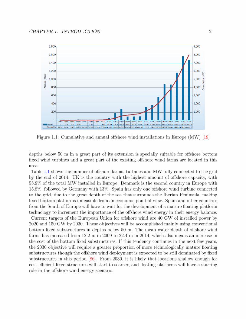
CHAPTER 1. INTRODUCTION 2
Figure 1.1: Cumulative and annual offshore wind installations in Europe (MW) [19]
depths below 50 m in a great part of its extension is specially suitable for offshore bottomfixed wind turbines and a great part of the existing offshore wind farms are located in thisarea.Table 1.1 shows the number of offshore farms, turbines and MW fully connected to the gridby the end of 2014. UK is the country with the highest amount of offshore capacity, with55.9% of the total MW installed in Europe. Denmark is the second country in Europe with15.8%, followed by Germany with 13%. Spain has only one offshore wind turbine connectedto the grid, due to the great depth of the sea that surrounds the Iberian Peninsula, makingfixed bottom platforms unfeasible from an economic point of view. Spain and other countriesfrom the South of Europe will have to wait for the development of a mature floating platformtechnology to increment the importance of the offshore wind energy in their energy balance.Current targets of the European Union for offshore wind are 40 GW of installed power by2020 and 150 GW by 2030. These objectives will be accomplished mainly using conventionalbottom fixed substructures in depths below 50 m. The mean water depth of offshore windfarms has increased from 12.2 m in 2009 to 22.4 m in 2014, which also means an increase inthe cost of the bottom fixed substructures. If this tendency continues in the next few years,the 2030 objective will require a greater proportion of more technologically mature floatingsubstructures though the offshore wind deployment is expected to be still dominated by fixedsubstructures in this period [86]. From 2030, it is likely that locations shallow enough forcost efficient fixed structures will start to scarcer, and floating platforms will have a starringrole in the offshore wind energy scenario.
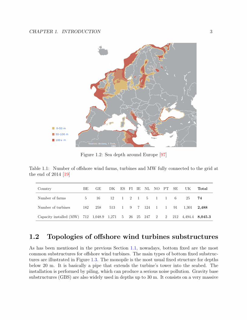
CHAPTER 1. INTRODUCTION 3
Figure 1.2: Sea depth around Europe [97]
Table 1.1: Number of offshore wind farms, turbines and MW fully connected to the grid atthe end of 2014 [19]
Country BE GE DK ES FI IE NL NO PT SE UK Total
Number of farms 5 16 12 1 2 1 5 1 1 6 25 74
Number of turbines 182 258 513 1 9 7 124 1 1 91 1,301 2,488
Capacity installed (MW) 712 1,048.9 1,271 5 26 25 247 2 2 212 4,494.4 8,045.3
1.2 Topologies of offshore wind turbines substructures
As has been mentioned in the previous Section 1.1, nowadays, bottom fixed are the mostcommon substructures for offshore wind turbines. The main types of bottom fixed substruc-tures are illustrated in Figure 1.3. The monopile is the most usual fixed structure for depthsbelow 20 m. It is basically a pipe that extends the turbine’s tower into the seabed. Theinstallation is performed by piling, which can produce a serious noise pollution. Gravity basesubstructures (GBS) are also widely used in depths up to 30 m. It consists on a very massive

CHAPTER 1. INTRODUCTION 4
Figure 1.3: Wind turbine fixed substructures main concepts. From left: monopile, gravitybase, tripod and jacket [6]
base that rests on the seabed providing stability to the structure connected to it. The mainadvantage of this structure is that it can be built at land and then towed to the locationand submerged by adding ballast. For depths higher than 30 m space frame substructures astripods or jackets are usually more cost efficient. These kind of substructures are composedof steel pipes. Tripods have a main central column with three legs that are driven into theseabed. Jackets are more transparent structures because there is no central column and,consequently, less steel is needed.Relating the floating wind turbines, three main topologies exist depending on how the
system stability is achieved. These three concepts are illustrated in Figure 1.4. In the spardesign, ballast is located in the lower part of the platform to bring down the center of gravityof the system below the center of buoyancy. If the platform is displaced from the verticalposition, a restoring moment created by gravity and buoyancy forces provides stability. Inthis type of platforms, the area that pierces the water surface is minimized to decrease theinteraction with the waves. Spars are typically easy to manufacture, but the large draft (canbe more than 100 m) can create logistic problems. In the semisubmersible concept, there isan important amount of volume of the platform at the water surface level. These volumesare clearly displaced from the platform center increasing the moment created by buoyancyforces and giving stability to the platform. The low draft of semisubmersibles simplifies theinstallation process. Finally, tension leg platforms (TLP’s) are relatively light platforms withrespect to its volume with an excess of buoyancy force that is compensated by the tensionof the mooring lines. TLP’s usually have a shallow draft and require less material to beconstructed, but the lines and the anchors experiment very high tensions. In addition, theinstallation process can be challenging and the failure of a tendon during the wind turbineoperation represents a critical incident.

CHAPTER 1. INTRODUCTION 5
Figure 1.4: Wind turbine floating platforms main concepts: spar (left), semisubmersible(center) and TLP (right). Source: DNV GL
1.3 Mooring lines topologies
Mooring systems are composed of mooring lines that are attached to the platform at a pointcalled fairlead and have the lower ends anchored to the seabed. Mooring systems are respon-sible of the station keeping of floating platforms, contributing to the stability in the case ofTLP designs.The lines can be made up of chain, wire or synthetic rope. The chain is the most commonmaterial in depths up to 300 m. For higher depths, wire rope can be more adequate becauseit is lighter and more flexible. The synthetic fiber rope is lighter than chain or wire, andis typically used in combination with them for mooring systems at deep waters (2000 m ormore).Basically, two main mooring configurations for the mooring systems exist: the catenarymooring systems, used in spar and semisubmersible concepts, and the taut-leg mooring sys-tems, used in TLP designs (see Figure 1.4). In addition, some platforms have adopted asemi-taut mooring system, which is a hybrid between the taut and the catenary moorings.The catenary is the most common mooring configuration and receives this name from theshape that a hanging chain or cable assumes under its own weight when it is supported

CHAPTER 1. INTRODUCTION 6
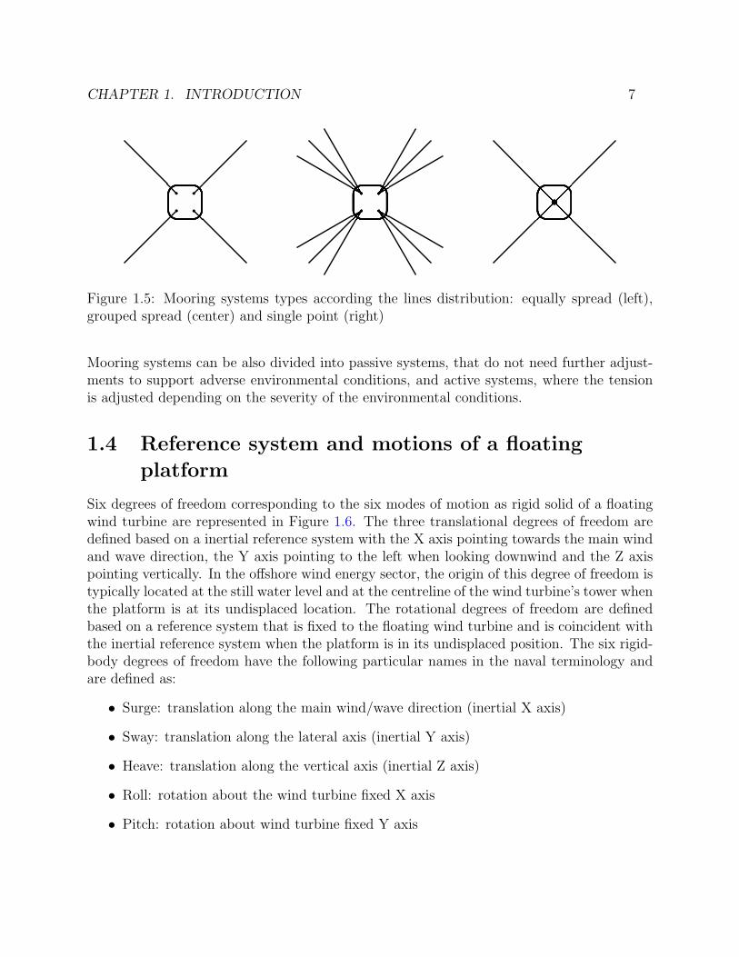
only at its ends. In catenary mooring systems, the lines are relatively long in comparisonwith the water depth and part of them are lying in the seabed. In consequence, the anchoronly experiments horizontal forces. The restoring forces in the catenary mooring systemsare generated by the gravity force acting on the suspended portion of the lines and by thechanges in the line shape due to the platform motion. As the water depth increases, thelength and the weight of the lines increases rapidly, becoming excessive for deep waters.In taut mooring systems, the lines are pre-tensioned and the restoring forces are generatedmainly through the axial stiffness of the mooring lines rather than by geometry changes.The stiffness of taut mooring systems is more linear than in catenary systems and allows abetter platform offset control under mean load. In addition, the mooring lines have to beelastic enough not to suffer overloading under the platform motions induced by the waves.Semi-taut mooring lines are a combination of taut moorings with catenaries. Semi-taut andtaut mooring systems require less seabed space and shorter lines than the catenary, resultingin material saving and smaller footprint. Although they need more expensive anchors dueto the high vertical loads and the installation procedure is challenging, it could be a morecost-efficient solution than the catenary system for high depth locations.Mooring systems can also be classified depending on the number of lines and their dis-tribution. Figure 1.5 represents the different types of mooring systems according to thedistribution of the lines. Most of the floating wind turbines designs use spread mooringsystems, that consist of multiple lines attached to the platform on several locations, usuallywith a symmetrical distribution. This configuration restricts the rotation of the structure inthe horizontal plane due to wind, waves and currents, providing an almost constant headingto the structure. The lines of a spread mooring system can be equally spread around thefloating structure or grouped. The grouped moorings provide better redundancy against thefailure of a line. Some floating wind turbines designs, in particular spars, have proposeda single point mooring system, where all the lines are connected to the same point of theplatform that is free to rotate in horizontal plane. In these cases the lines are sometimes at-tached to a turret with bearings to allow the structure rotation. This configuration allows thesystem to adjust to the prevailing environment, minimizing loads in harsh multi-directionalenvironments.
CHAPTER 1. INTRODUCTION 7
Figure 1.5: Mooring systems types according the lines distribution: equally spread (left),grouped spread (center) and single point (right)
Mooring systems can be also divided into passive systems, that do not need further adjust-ments to support adverse environmental conditions, and active systems, where the tensionis adjusted depending on the severity of the environmental conditions.
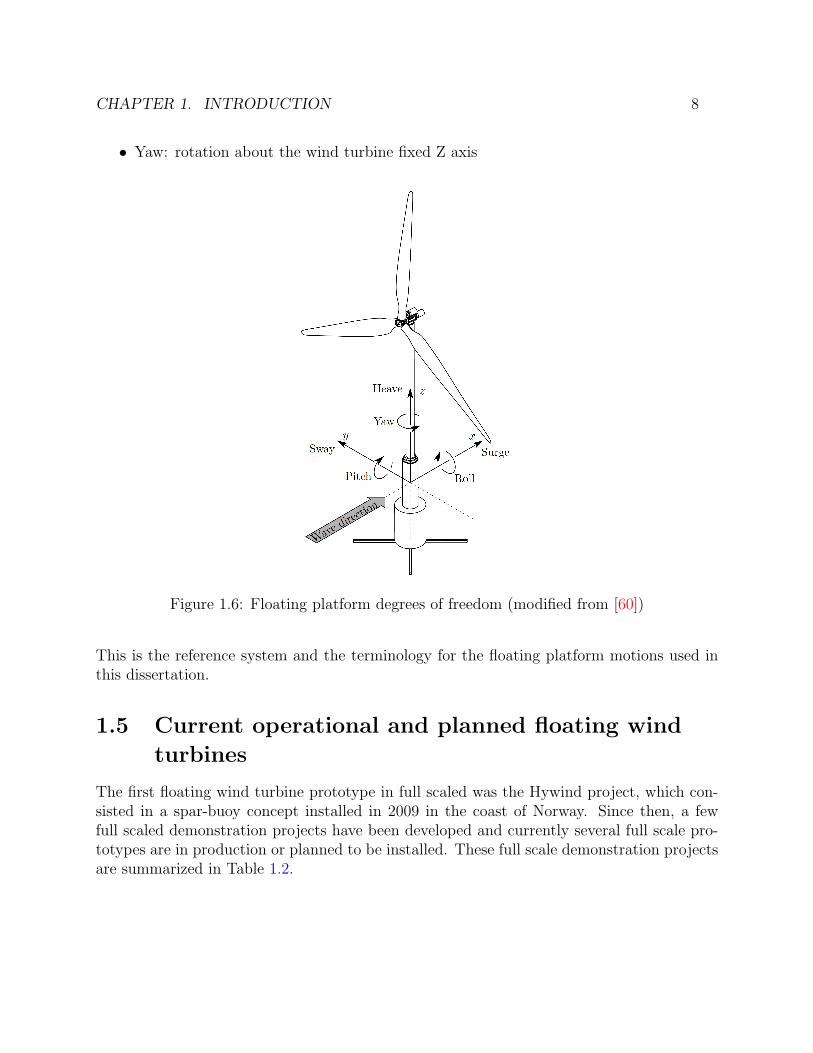
1.4 Reference system and motions of a floating
platform
Six degrees of freedom corresponding to the six modes of motion as rigid solid of a floatingwind turbine are represented in Figure 1.6. The three translational degrees of freedom aredefined based on a inertial reference system with the X axis pointing towards the main windand wave direction, the Y axis pointing to the left when looking downwind and the Z axispointing vertically. In the offshore wind energy sector, the origin of this degree of freedom istypically located at the still water level and at the centreline of the wind turbine’s tower whenthe platform is at its undisplaced location. The rotational degrees of freedom are definedbased on a reference system that is fixed to the floating wind turbine and is coincident withthe inertial reference system when the platform is in its undisplaced position. The six rigid-body degrees of freedom have the following particular names in the naval terminology andare defined as:
• Surge: translation along the main wind/wave direction (inertial X axis)
• Sway: translation along the lateral axis (inertial Y axis)
• Heave: translation along the vertical axis (inertial Z axis)
• Roll: rotation about the wind turbine fixed X axis
• Pitch: rotation about wind turbine fixed Y axis
CHAPTER 1. INTRODUCTION 8
• Yaw: rotation about the wind turbine fixed Z axis
Figure 1.6: Floating platform degrees of freedom (modified from [60])
This is the reference system and the terminology for the floating platform motions used inthis dissertation.
1.5 Current operational and planned floating wind
turbines
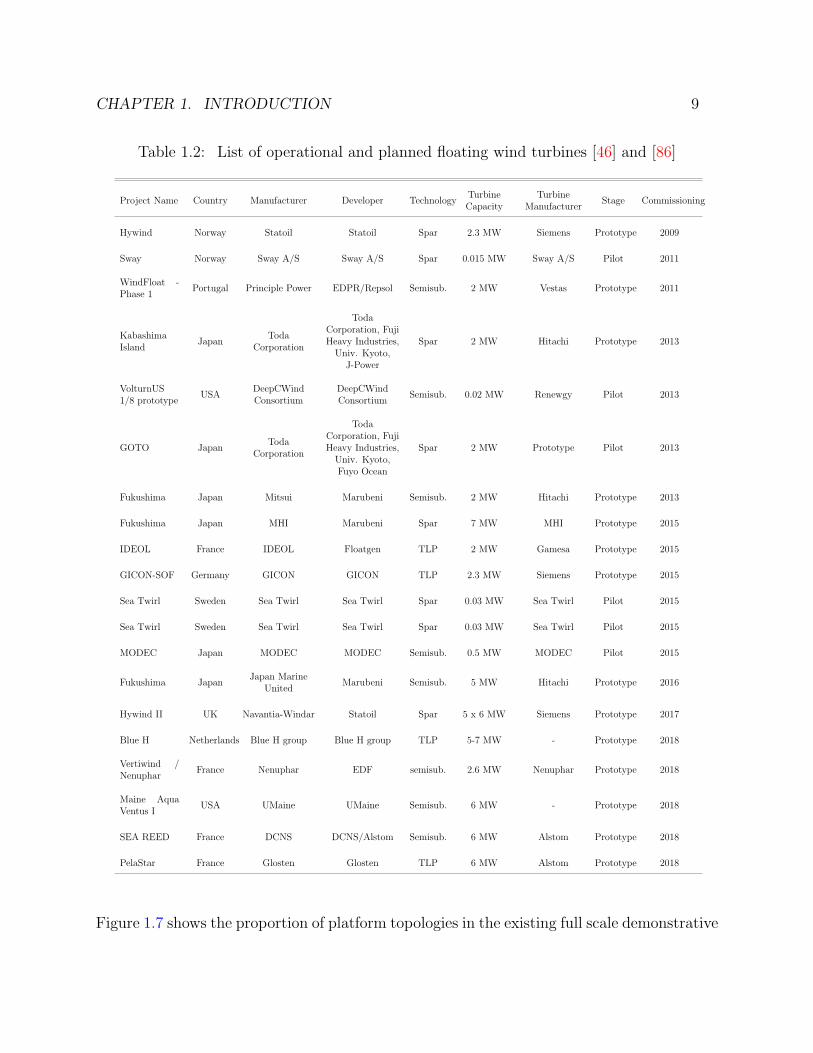
The first floating wind turbine prototype in full scaled was the Hywind project, which con-sisted in a spar-buoy concept installed in 2009 in the coast of Norway. Since then, a fewfull scaled demonstration projects have been developed and currently several full scale pro-totypes are in production or planned to be installed. These full scale demonstration projectsare summarized in Table 1.2.
CHAPTER 1. INTRODUCTION 9
Table 1.2: List of operational and planned floating wind turbines [46] and [86]
Project Name Country Manufacturer Developer TechnologyTurbineCapacity
TurbineManufacturer
Stage Commissioning
Hywind Norway Statoil Statoil Spar 2.3 MW Siemens Prototype 2009
Sway Norway Sway A/S Sway A/S Spar 0.015 MW Sway A/S Pilot 2011
WindFloat -Phase 1
Portugal Principle Power EDPR/Repsol Semisub. 2 MW Vestas Prototype 2011
KabashimaIsland
JapanToda
Corporation
TodaCorporation, FujiHeavy Industries,Univ. Kyoto,
J-Power
Spar 2 MW Hitachi Prototype 2013
VolturnUS1/8 prototype
USADeepCWindConsortium
DeepCWindConsortium
Semisub. 0.02 MW Renewgy Pilot 2013
GOTO JapanToda
Corporation
TodaCorporation, FujiHeavy Industries,Univ. Kyoto,Fuyo Ocean
Spar 2 MW Prototype Pilot 2013
Fukushima Japan Mitsui Marubeni Semisub. 2 MW Hitachi Prototype 2013
Fukushima Japan MHI Marubeni Spar 7 MW MHI Prototype 2015
IDEOL France IDEOL Floatgen TLP 2 MW Gamesa Prototype 2015
GICON-SOF Germany GICON GICON TLP 2.3 MW Siemens Prototype 2015
Sea Twirl Sweden Sea Twirl Sea Twirl Spar 0.03 MW Sea Twirl Pilot 2015
Sea Twirl Sweden Sea Twirl Sea Twirl Spar 0.03 MW Sea Twirl Pilot 2015
MODEC Japan MODEC MODEC Semisub. 0.5 MW MODEC Pilot 2015
Fukushima JapanJapan Marine
UnitedMarubeni Semisub. 5 MW Hitachi Prototype 2016
Hywind II UK Navantia-Windar Statoil Spar 5 x 6 MW Siemens Prototype 2017
Blue H Netherlands Blue H group Blue H group TLP 5-7 MW - Prototype 2018
Vertiwind /Nenuphar
France Nenuphar EDF semisub. 2.6 MW Nenuphar Prototype 2018
Maine AquaVentus I
USA UMaine UMaine Semisub. 6 MW - Prototype 2018
SEA REED France DCNS DCNS/Alstom Semisub. 6 MW Alstom Prototype 2018
PelaStar France Glosten Glosten TLP 6 MW Alstom Prototype 2018
Figure 1.7 shows the proportion of platform topologies in the existing full scale demonstrative

CHAPTER 1. INTRODUCTION 10
projects. The distribution between the three main topologies is balanced, with a slightprevalence of semisubmersibles.
Spar 33%
Semisubmersible 44%
TLP 23%
Figure 1.7: Platform topologies in demonstrative full scale floating wind turbine projects
1.6 Design standards for floating structures
The companies that develop new technologies as floating wind turbines are usually reluc-tant to share sensitive information or lessons learned. The development of standards forthe design of offshore floating structures allows to establish a consensus in the industry ondesign principles that considers the experience of engineers and companies. The applicationof the guidelines that consider the particular aspects of floating wind turbines facilitates theeconomical optimization of the designs.DNV GL has developed the DNV-OS-J103 standard [27] that is specific for the design offloating wind turbines. This guideline was defined within an industry joint project between2011 and 2013 with the participation of some of the most relevant actors of the sector suchas: Alstom, Gamesa, Statoil-Hydro, Glosten Associates, Sasebo Heavy Industries, Princi-ple Power, Iberdrola, Navantia, STX Offshore & Shipbuilding, and Sumitomo Metal. Thisstandard has to be complemented with the more general guideline DNV-OS-J101 [26] andtogether provide a set of principles, technical requirements and guidance for the design, theconstruction, the inspection during the service and the transportation. In addition, specificstandards exist for the design of tendons [24] and mooring lines [25].DNV GL standards are mainly used in Europe. In America, an equivalent set of guidelineshas been developed by the American Bureau of Shipping (ABS), providing guidance in si-milar aspects of the design process.The IEC 61400 standards are published by the International Electrotechnical Commission(IEC), regarding wind turbines. They define the design requirements to ensure that windturbines are correctly engineered against damage from hazards during their lifetime. The

CHAPTER 1. INTRODUCTION 11
IEC 61400-3 Edition 1 [47] is the most commonly used standard for the calculation of loadsfor offshore wind turbines. Nevertheless, this guideline states that the loadcases describedmay not be sufficient for the design of floating wind turbines. IEC has been working on theIEC 61400-3 Edition 2 guideline that will include more specific load cases for floating windturbines including damage stability (flooded compartment), line loss, second-order hydrody-namics, etc.
1.7 Integrated codes for offshore wind turbines
The load calculation of floating offshore wind turbines requires time-domain simulation toolscapable of accounting for all the phenomena that affect the system: aerodynamics, structuraldynamics, hydrodynamics, control actions and the mooring lines dynamics. These effectspresent couplings and are mutually influenced. The computational tools able to computethese coupled effects are called integrated or coupled codes. Some literature also refers tothese tools as aero-hidro-servo-elastic codes.The integrated codes for the simulation of floating wind turbines use different approachesto describe the mooring system behaviour coupled with the platform motions. Some ofthem are simplified methods, such as the quasi-static approach or the force-displacementrelationships. Other models represent the full dynamics equations of the lines, consideringeffects as inertia, added mass or the water-line drag that are not captured by the simplifiedmethods, though this means a higher computational effort. A more detailed description ofthe integrated codes and mooring models is provided in Chapter 3.
1.8 Motivation for this research
Several studies have pointed out the need of dedicated and comprehensive studies of thedynamics of mooring lines specifically focusing on coupled codes for floating wind turbines,see for example [72] and [70]. The fatigue and ultimate loads provided by integrated tools areused for the structural design of the different components of the wind turbine, consequentlytreated as inputs for the structural computation performed by finite element method (FEM).The level of loads has a great influence on the design of the components. For this reason,the accuracy and reliability of the integrated simulation codes, including the mooring systemmodels, are important to achieve optimized and cost-effective floating wind turbine designsthat can make possible the objectives of the European Union for offshore wind energy for2030. Nevertheless, it has to be kept in mind that the accuracy of the tools has to bebalanced with a reasonable computational cost of the simulation tools to have an efficientdesign procedure.In this context, this research will be focused on how dynamics of the mooring lines can be

CHAPTER 1. INTRODUCTION 12
considered in the integrated simulations for the design of offshore wind turbines and if theinclusion of these dynamic effects is relevant for the computation of the fatigue and extremeloads.
13
Chapter 2
Objectives and methodology
2.1 Objectives
The objective of this dissertation is to investigate computational and experimental metho-dologies to evaluate mooring dynamics and implement them in integrated codes for thesimulation of floating wind turbines. With these tools, conclusions on the applicability ofmooring dynamics to the design of floating wind turbines will be obtained.In particular, the following goals are pursued in this research:
• Improvement of integrated simulation tools for floating wind turbines by developingdynamic mooring lines models
• Development, implementation and verification of mooring lines testing methodologies
• Validation of simulation tools for mooring dynamics against experimental data
• Validation of the coefficients for computation of drag forces in chains provided by theguidelines
• Evaluation of the influence of mooring dynamics on the fatigue and ultimate loads cal-culated for different floating wind turbine concepts according to certification guidelines
The development of accurate and verified simulation tools will provide more exact loadsto design the floating wind turbine components, contributing to the optimization of thestructure and to the cost reduction. In addition, the characterization of the impact of themooring dynamics on the results of the simulation tools will allow designers to choose whenthese effects should be considered or when lower complexity tools can be used, thus savingcomputational time.

CHAPTER 2. OBJECTIVES AND METHODOLOGY 14
2.2 Methodology
The following tasks, that will be described in the next chapters, have been performed tofulfill the objectives enumerated in the previous Section 2.1:
• In Chapter 3 a revision on the current state of development of integrated codes forfloating wind turbines is provided with particular attention to their capabilities on thesimulation of mooring dynamics. The existing studies performed on the experimentalvalidation of mooring line codes are also reviewed. Finally, past studies on the influ-ence of mooring dynamics on the loads of floating wind turbines are examined. Thisbibliographic revision served as a starting point for this research, identifying the needsof development and research that are subsequently carried out in Chapters 4, 5 and 6.
• In Chapter 4 a dynamic mooring line code based on a lumped mass formulation isdeveloped. The non linear equations of motion of a line are discretized using the finiteelement method and solved in the time domain. The equations are implemented in acode called OPASS (Offshore Platforms Anchorage System Simulator). The OPASScode is coupled with the FAST code [50] for integrated simulations of floating windturbines.
• The dynamic mooring line code is experimentally validated in Chapter 5. The expe-riment setup consists of a chain submerged with one end anchored at the bottom ofthe basin and the suspension point at the still water level. The suspension point isexcited with a prescribed periodic motion at different frequencies and for two confi-gurations of the line. The tension at the fairlead and the motion at several positionsalong the length of the line are measured and compared with the numerical predictionsof equivalent simulation cases.
• Chapter 6 quantifies the influence that the inclusion of mooring dynamics has onthe calculation of fatigue and ultimate loads for floating wind turbines. The OPASScode coupled with FAST is used to compute the loads including mooring dynamics.These results are compared with the loads calculated also with FAST but using alower complexity quasi-static approach. The computation of the loads is done for thethree main existing floating wind turbines topologies (semisubmersible, spar-buoy andtension leg platform), following the IEC 61400-3 guideline [47] and according to themethodologies required by the certification entities within the offshore wind energyindustry. More than 20,000 simulation cases are launched and postprocessed for thisstudy.
• Finally, the conclusions of this research and the future lines of work are presented inChapter 7.
15
Chapter 3
State of the art
3.1 Overview on integrated codes for floating wind
turbines
The introductory Chapter 1 highlighted the importance of accurate and reliable integratedsimulation tools for the cost-efficient design of floating wind turbines. The simulation of thedynamics of a floating wind turbine has to integrate all the phenomena that can influencethe behaviour of the system as aerodynamics, hydrodynamics, control, structural dynamics,mooring line dynamics, etc. Each of these effects is mutually influenced and a reliable cal-culation should evaluate them in a coupled way.Several studies relating floating wind turbines reveal that the dynamics of the mooringsgreatly affects the tension of the lines and can influence the fatigue and extreme loads ofthe turbine components (see Section 3.4). An accurate simulation of the mooring systemwithin the integrated codes can be fundamental for the optimization of the final floatingwind turbine design.The aero-servo-hydro-elastic codes are composed of different submodels representing all thephysics that affect the wind turbine dynamics, such as the external conditions (wind andwaves), the aerodynamics, the structural dynamics, the hydrodynamics or the dynamics ofthe mooring lines, taking also into account the wind turbine control strategy. The followingsubsections give an overview of the models used in the integrated codes.
3.1.1 External conditions
The external conditions that affect a floating wind turbine are the wind loading, the wavesand the currents. The codes have to generate the wind inflow including a wide varietyof conditions: steady wind, turbulent winds, gusts, vertical shear, direction changes, etc.Different turbulent models such as Von Karman [29], Kaimal [52] or Mann [67] are usually
CHAPTER 3. STATE OF THE ART 16
available in the codes.For the wave conditions, the codes have to generate regular and irregular waves with differentperiods and heights. Airy theory is widely used to describe linear waves (see, for example,[32] or [77]). It produces sinusoidal sea surface elevation but does not provide any informationabout the kinematics over the medium sea level. Several methods exist to extrapolate thewave kinematics to the actual sea surface called stretching methods (see, for example, [21]).Some codes generate waves including second order effects to describe higher amplitude wavesor low sea depth situations. Stream function is a wave theory that describes highly non-linear waves up to the breaking limit [23].Currents are included in the described models as they could have great influence on thesystem response. These currents can be near-surface or sub-surface and include differentprofiles to define the variation of the velocity with depth.
3.1.2 Aerodynamics models
The most widely used model for the calculation of the aerodynamic loads in integrated codesis the Blade Element Method (BEM) (see for example: [90] or [17]). In this approach, theblade is divided into elements independent from the adjacent elements, where the forcesare calculated using the airfoil lift and drag coefficients. The calculation does not considertri-dimensional effects along the blade. Inertial effects of the flow are not taken into account.To overcome the model limitations, several semi-empirical corrections are typically appliedto the results to take into consideration the hub and the blade tip losses [36], the yaw mis-alignment [35], high induction factors [35] or the effect of unsteady aerodynamics (dynamicstall) [61].Some codes also apply the Generalized Dynamic Wake (GDW) theory [100] that is basedon potential theory and is able to describe the pressure distribution over the rotor includingthree-dimensional and unsteady effects.Free-wake 3D modelling using vortex particle dynamics has been implemented in some in-tegrated tools [3]. This approach assumes a potential flow field around the airfoil that isdescribed through the distribution of discrete sources and vortices. Like BEM, forces arebased on lift and drag coefficients data of the profile that are corrected considering the effectsof blade rotation. It is expected that this theory provides better simulations in conditionswhere the wake dynamics is important or when there is a strong time dependency of theaerodynamic characteristics, as in flow misalignments.
3.1.3 Hydrodynamics models
There are two main hydrodynamic models that can be applied for the computation of theloads in the substructure: models based on the Morison equation and the potential theory.Morison equation [75] is applicable to slender bodies. Basically, this load calculation methodis based on the use of two coefficients: the inertia and the drag coefficients. To achieve a
CHAPTER 3. STATE OF THE ART 17
correct prediction of the loads these coefficients have to be carefully chosen or derived fromavailable experimental data.The linear potential theory (see, for example, [32] or [77]) is a more advanced approachthat can be applied to any geometry, but it neglects the viscous drag effect. From thecomputational point of view, it is more time-consuming than the Morison approach. Themissing part of the damping due to viscous mechanisms can be included in time domain usingthe drag term of the Morison equation or increasing the overall platform damping with linearand quadratic damping matrices derived from experiments. The potential theory implies theresolution of the Laplace equation for the fluid domain. The boundary element method canbe applied to solve the equation both in the frequency domain [103] or in the time domain[108]. The hydrodynamic coefficients provided by the frequency domain solution can be alsoused as inputs for time domain simulations, as in [50]. The potential hydrodynamic problemcan be also directly solved in time domain using the finite element method [93], [92]. Thismethod is more efficient when high number of unknowns are involved as in ocean engineeringproblems with many freely floating bodies. The potential linear theory can be extended totake into account second order hydrodynamic effects [85] that can have an important rolein the dynamics of certain floating platform concepts, particularly semisubmersibles, as it isdemostrated in [66] and [15].
3.1.4 Structural dynamics models
Some codes use a modal approach [104] for the dynamics of the flexible bodies that composethe wind turbine structure. It consists on a reduction of the degrees of freedom of the flexiblebodies to a limited amount of modal degrees of freedom. The motion of the flexible body isobtained by the linear combination of the body modes multiplied by the modal degrees offreedom. This approach is linear and, therefore, it cannot represent large deflections wherenon-linearities arise, such as the ones in the long blades typically used in offshore windturbines.Other approaches as finite element method (FEM) or multi-body systems are able to capturenon-linear effects due to large deflections, though they have a higher computational cost.
3.1.5 Control
Most of the codes allow setting the parameters of very simple pitch control and rotor variablespeed strategies. More advanced control strategies are usually implemented in dynamic linklibraries (DLLs) and interfaced with the code.
3.1.6 Mooring line modeling approaches
The equations of motion of a submerged line are non-linear and cannot be solved analytically.Instead, either simplified approaches or numerical methods are applied. Simplified methods
CHAPTER 3. STATE OF THE ART 18
as the quasi-static approach [50] or the force-displacement relationships (for example in [87])are widely used in integrated codes, because they provide the computational efficiency re-quired for the simulation of the thousands of load cases requested by the guidelines. Theproblem of solving the full dynamic representation of the lines requires a much higher com-putational effort and can be approached using different techniques. The fundamentals of themain mooring line models can be briefly described as:
• Quasi-staticThe static equations of the catenary at every time step of the simulation are solved,given the position of the fairlead where the line is attached to the platform. This modeltypically accounts for weight and buoyancy, axial stiffness, and friction from variablecontact on the seabed, but does not consider the inertial effects, the hydrodynamicdrag from waves, currents or the relative motion of the line within the fluid field.
• Force-displacement relationshipIn this model, non-linear spring stiffnesses are applied to the translational and rota-tional degrees of freedom of the platform. The force-displacement relationship has tobe derived using a line analysis code and the results obtained would be similar to thequasi-static approach.
• Dynamic modelThis approach considers dynamic effects as inertia, added mass or hydrodynamic drag.Several formulations have been developed that can handle the dynamics of the line,such as FEM, finite difference method or multi-body models. The lumped mass modelcan be considered a variation of the FEM approach, where the mass of the elements isconcentrated in the element’s adjacent nodes.
3.2 Revision of mooring line models in simulation
codes
In this Section, the available integrated codes for the simulation of floating wind turbinesare reviewed with particular attention to their mooring line modelling approaches. First,codes with simplified moorings models are described. Second, codes for floating structuresincluding dynamic mooring models with a wind turbine model are discussed analyzing theirfeatures and limitations. Finally, specific codes for mooring lines are also commented.

CHAPTER 3. STATE OF THE ART 19
3.2.1 Codes for the simulation of floating wind turbines withsimplified mooring line models
BLADED [16] is one of the most popular commercial codes for the simulation of wind tur-bines. It has been developed by Garrad Hassan, originally for the simulation of onshorewind turbines. It has been extended to model floating structures using Morison equationfor the computation of the hydrodynamic loading. In BLADED, the mooring lines are in-cluded through non-linear force-displacement relationships applied to the platform degreesof freedom. The aerodynamics of the rotor are based on BEM theory and, for the structuraldynamics, a modal approach has been implemented. The modes of the tower and the bladesare calculated internally using a multi-body model.The HAWC2 code [58] was developed by Risœ-DTU and applies the BEM theory for theaerodynamics and the Morison equation for the hydrodynamics. A multi-body formula-tion is used for the structural dynamics and the mooring lines are represented by a force-displacement relationship.The code FAST [50] is an open-source and free publicly available software developed byNREL. FAST allows the integrated simulation of onshore wind turbines and also offshorewind turbines both with a monopile or a floating substructure. The structural dynamics ismodelled using a combined modal and multi-body approach. The aerodynamics is basedon the BEM theory and is solved by a module called AeroDyn [4]. The hydrodynamics offloating platforms is calculated by the module HydroDyn using potential theory in time do-main. HydroDyn uses the wave forces and radiation coefficients computed by the boundaryelement method code WAMIT [107] in frequency domain as inputs. Quadratic drag basedon the Morison equation can be added to take into account for the viscous forces. A dragcoefficient along the vertical centreline of the platform has to be defined. Until version 7,the mooring lines model is a quasi-static approach. The recently launched version 8 presentsmore advanced mooring models that will be described in the next subsection.
3.2.2 Codes for the simulation of floating wind turbines withdynamic mooring line models
Most of the tools for floating platforms with capabilities for the modelling of mooring dy-namics were originated in the oil and gas industry and do not represent accurately the overallintegrated dynamics of the complete system because they tend to simplify the coupling withthe wind turbine dynamics [72]. On the other hand, many aeroelastic tools created for thesimulation of wind turbines lack of full capabilities for the computation of the different floa-ting platform topologies including the mooring lines dynamics.For this reason, most of the advanced tools for the integrated simulation of floating windturbines with mooring dynamics are the result of coupling between codes independently de-veloped. Each of these codes covers different parts of the complete problem, such as the

CHAPTER 3. STATE OF THE ART 20
hydrodynamics, the mooring dynamics or aerolasticity of the wind turbine.Table 3.1 summarizes the existing codes for the integrated simulation of floating wind tur-bines that include the dynamic simulation of the mooring system. Although most of thesetools are the result of coupling several independent codes, there are also a few tools thathave been developed specifically for the simulation of floating wind turbines.

CHAPTER 3. STATE OF THE ART 21
Table 3.1: Summary of floating wind turbines simulation tools including mooring dynamicsDesign
CodeNam
eCodeDevelop
erMooring
Dynam
ics
Cou
pled
Codes
for
Hydrody-
nam
ics
Hydrodynam
ics
Formulation
Cou
pledCodefor
Aerodynam
ics
Aerodynam
ics
Formulation
Dynam
icStall
Cou
pledCode
forW
TStructural
Dynam
ics
WT
structural
Dynam
ics
Cou
pling
Develop
erReferences
OrcaF
lex
Orcina
FEM
(LM)
-PF+QD+CD/
PF+ME/M
EFAST
BEM/G
DW
yes
FAST
Modal-
MBS
Orcina
[68]
CHARM3D
Texas
A&M
University
&OffshoreDynam
ics
Inc.
FEM
-PF+ME
FAST
BEM/G
DW
yes
FAST
Modal-
MBS
FAST
[94]
SIM
ORIFLEX
Marintek
FEM
-PF+ME
HAWC2
BEM
yes
HAWC2
MBS
Risøe
&Hydro
Oil&
Energy
[59],[96]
SIM
ORIFLEX
Marintek
FEM
-PF+ME
BEM
yes
-MBS
-[ 33]
SIM
ORIFLEX
Marintek
FEM
-PF+ME
AeroD
yn
BEM/G
DW
yes
-MBS
CeSOS&
NTNU
[80]
ANSYS
Aqwa
ANSYS,Inc.
FEM
-PF+ME
FLEX5
BEM
yes
FLEX5
Modal-
MBS
ANSYS,Inc.
-
DeepLines
Principia
FEM
-PF+QD/M
EInternal
DLL
BEM
yes
-FEM
IFPEN
[88]
aNySim
PHATASpro
MARIN
MBS
-PF+ME
PHATAS
BEM
yes
PHATAS
Modal-
MBS
MARIN
&ECN
-
SIM
PACK
SIM
PACK
AG
MBS
HydroDyn
PF+QD
AeroD
yn
BEM/G
DW
yes
-MBS
University
ofStuttgart
[71]
ProteusD
sUniversity
ofVictoria
&Dynam
icSystem
sAnalysisLtd.
FEM
(LM)
FAST
(HydroDyn)
PF+QD
FAST
(AeroD
yn)
BEM/G
DW
yes
FAST
Modal-
MBS
University
ofVictoria
[40]
3DFloat
IFE
FEM
-ME
-BEM
no
-FEM
-[78]
Hydro-
GAST
NTUA
FEM
-PF+ME
-BEM/F
WV
yes
-FEM
-[9]
MLTSIM
Technip
FEM
FAST
(HydroDyn)
PF+QD
FAST
(AeroD
yn)
BEM/G
DW
yes
FAST
Modal-
MBS
-[56]
FAST
v8/
FEAMoor-
ing
Texas
A&M
University
FEM
FAST
(HydroDyn)
PF+QD
FAST
(AeroD
yn)
BEM/G
DW
yes
FAST
Modal-
MBS/
FEM
Texas
A&M
University
[14]
FAST
v8/
MoorDyn
University
ofMaine
FEM
FAST
(HydroDyn)
PF+QD
FAST
(AeroD
yn)
BEM/G
DW
yes
FAST
Modal-
MBS/
FEM
University
ofMaine
[40]
BEM:BladeElementMom
entum
CD:Coeffi
cientof
DragQD:Quad
raticDragGDW
:Generalized
Dynam
icWakeFEM:FiniteElementMethodLM:Lumped
MassPF:Potential
Flow
ME:Morison
Equation
FW
V:FreeWakeVortexMBS:Multi-BodySystem
CHAPTER 3. STATE OF THE ART 22
OrcaFlex [79] is a commercial software developed by Orcina for the dynamic analysis ofoffshore structures, including catenary systems as mooring lines, flexible risers or umbilicalcables. Orcina has coupled OrcaFlex with the FAST code [68]. In the resulting tool, FASTis responsible for the simulation of aerodynamics, the control system and the structuraldynamics of flexible elements, such as the rotor and the tower. OrcaFlex computes the hy-drodynamics of the platform using an analogous approach to HydroDyn and also considersthe dynamics of the mooring system.Similarly, FAST has been used to model the wind turbine in a coupling with the CHARM3Dcode that computes the floating body and the mooring system dynamics [94]. CHARM3Dis a code for purchase developed by Texas A&M and Offshore Dynamics, Inc. for the simu-lation of moored floating structures, but has not capabilities for the coupled aerodynamics,the structural dynamics and the control actions of a wind turbine.SIMO/RIFLEX is one of the leading software for the analysis of offshore structures. Histori-cally, it has been widely used in the oil and gas industry. RIFLEX is a finite element modulefor the dynamic analysis of mooring lines and SIMO is the module that performs the timedomain hydrodynamic analysis of the floating platform, using potential theory. Morisonelements can also be included. A module for the calculation of the aerodynamic forces onthe wind turbine rotor based on the BEM theory has been developed [33]. The forces at theblade elements are integrated and the resulting 3 forces and 3 moments are applied to theSIMO model as a user-specified external load.The SIMO/RIFLEX code has also been coupled with HAWC2 for the inclusion of the windturbine’s aerodynamic loading. This coupling has been implemented by Risœ and Hydro Oil& Energy [59], [96].ANSYS Aqwa is a general purpose software for the analysis of offshore structures. Themooring system can be modeled using finite element theory. ANSYS, Inc. has coupledhis software with the code FLEX5 but neither the tool nor the documentation are publiclyavailable. FLEX5 is a code created by DTU for the aeroelastic computation of onshore windturbines. It is based on the BEM theory and uses a modal representation of the flexiblebodies.DeepLines is a general code for the simulation of offshore structures based on the poten-tial theory or, alternatively, the Morison equation. It includes the dynamic analysis of themooring system. Currently, PRINCIPIA, the company owner of the code, is collaboratingwith IFPEN (Institut Franais du Petrole - Energies Nouvelles) adding to the code capabi-lities for the simulation of floating wind turbines. The rotor aerodynamic model is basedon the BEM theory and is coupled with the DeepLines code through a DLL generated byIFPEN. A preliminary verification of the tool has been performed within the IEA Annex 30(OC4).The integrated tool aNySimPHATASpro, developed by MARIN, is the result of the couplingof the code aNySimpro and PHATAS [65]. aNySim has been developed by MARIN for theanalysis of offshore structures and is able to consider the mooring dynamics using a multi-body formulation. PHATAS is a code developed by ECN for the aeroelastic simulation of
CHAPTER 3. STATE OF THE ART 23
onshore wind turbines.SIMPACK is another commercial software for the dynamic simulation of mechanisms widelyused in many different industrial sectors. It is a general purpose program that has beenapplied by the University of Stuttgart to model the structural dynamics of a floating windturbine, including the mooring lines. The aerodynamics and hydrodynamics have been in-troduced in the model by coupling with SIMPACK the NREL’s AeroDyn and HydroDyncodes [71].ProteusDS [41]is a specific software for the dynamic analysis of mooring lines, using a finiteelement formulation with the mass of the cable lumped at the nodes. It has been develo-ped by the University of Victoria and Dynamic Systems Analysis Ltd. ProteusDS has beencompiled as a DLL and then coupled with the FAST code.The MLTSIM code [56], developed by Technip, is a finite element based code that has beencoupled with FAST. The coupled tool MLTSIM-FAST has been experimentally validatedagainst wave tank tests [57].There are also a few specialized codes that have been originally conceived for the simulationof offshore floating wind turbines including the mooring dynamics.3DFloat is an specific code for the integrated analysis of onshore and offshore wind turbines,including mooring system dynamics. It has been developed by IFE [78] and uses the BEMtheory for the aerodynamics, the finite element method for the structural and mooring linedynamics and the Morison equation for the hydrodynamics.Hydro-GAST is another integrated code developed by NTUA that uses potential theory forthe hydrodynamics, the BEM theory or, alternatively, the Free Wake Vortex theory for theaerodynamics and a finite element formulation for the mooring lines and structural dynamics[3], [9].Recently, NREL has launched the new FAST version 8 that includes the coupling with twodynamic mooring line codes: FEAMooring [14], based on finite element theory, and MoorDyn[40], which is a lumped mass formulation.
3.2.3 Other specific codes for the dynamic analysis of mooringlines
Many other programs specific for the simulation of the dynamics of mooring lines exist, butthey do not have capabilities for the simulation of the rest of components of a floating windturbine and they have neither been coupled with other tools for this purpose, although thiscould be done in the future. Some examples of specific codes for mooring lines based on thefinite element method are: MDD (Mooring Design and Dynamics) (Centre for Earth andOcean Research, University of Victoria) [28], Ariane7 (VeriSTAR) [7], CABLE3D (TexasA&M), Flexcom V8 (MCS Kenny), HYBER (USFOS) [44] and SeaDyn (US Navy) [109].Compass Ingenierıa y Sistemas and CIMNE (Centro Internacional de Metodos Numericosen la Ingenierıa) have developed the SeaFEM code [102], a time domain code for floating
CHAPTER 3. STATE OF THE ART 24
bodies that solves the hydrodynamic potential equations with finite element method. Thiscode has been recently coupled with a finite element dynamic mooring model [39]. Thecode LINES, developed by the Massachusetts Institute of Technology (MIT), is based on amulti-body formulation. The Massachusetts Institute of Technology, together with WoodsHole Oceanographic Institute has also developed the WHOIcable code [37], that is based onthe finite difference method. This code is publicly available.
3.3 Revision of previous experimental validations of
dynamic mooring line codes
The achievement of reliable simulation tools requires the validation of the computationalpredictions with experimental results. An experimental validation of the dynamic mooringline code developed in this research is part of the methodology to achieve the objectives ofthe study. The previous work performed in the past on the validation of dynamic mooringlines is summarized in this section.The lumped mass method was first used to model a mooring line at the end of the 50’s[106], although the model was simple and neglected the elasticity of the material, the hy-drodynamic drag forces or the seabed-line contact and the model was not validated. Thismodel was improved at the beginning of the 80’s including elasticity, seabed-line interactionand drag due to the relative motion of the cable with respect to the water. This methodwas validated with forced harmonic oscillation tests in [110] and [76]. The agreement withcomputational models was good, though the tests only covered a limited set of cases that didnot consider slack conditions. The methodology to perform the experimental tests was basedon the work described a few years before in [84]. During the 80’s decade other lumped massmodels were built as [55] and [64] and new approaches based on finite difference method [91]or finite element method [48] were developed. More recently, other formulations based onlinear finite element methods [2], higher order finite elements [30] and mixed finite elementformulations [73] have been presented. Some research on dynamic finite element models forpolyester mooring lines has also been performed [101].A comparison between a computational lumped mass model and a submerged line with pres-cribed harmonic displacements at the suspension point is described in [105]. This referenceshows a good agreement at the line fairlead tension between the experimental results andthe calculation, but comparisons of the cases including slack condition are not shown.In [99], the experimental results of the different line configurations are classified in four diffe-rent conditions. In the Quasi-Static Condition, the frequency of the excitation is low and thedynamic effects are negligible. The Harmonic Condition appears at a higher frequency andpresents a tension signal in time domain that is close to sinusoidal. In the Snap Condition,the tension drops to zero when the fairlead moves towards the anchor. When the motionreverses, the tension is recovered, and the zero loaded chain links that are falling suddenly
CHAPTER 3. STATE OF THE ART 25
stop and a snap loading is produced. The fourth condition appears when the excitationfrequency increases even more and the upper end of the chain completes a period before thewhole chain is able to respond. In this case, a lower number of chain links loose tensionand the snap load amplitudes start decreasing again. In the same reference, a lumped massmodel is compared with tension experimental results with good agreement for the HarmonicCondition, but presents significant differences when the line loses tension.The importance in the mooring line dynamic modelling of the accurate identification ofthe cable elastic stiffness and the free falling velocity is highlighted in [83]. This work alsopresents a comparison between the experimentally measured tension and numerical computa-tions showing good agreement. In [95], dynamic simulations with Orcaflex [79] are comparedto experimental data of a mooring line with prescribed harmonic motion of the fairlead. Theline tested consisted of a chain - steel wire rope - chain line and the Orcaflex numericalmodel included the bending stiffness for the wire rope. The experiments include cases withand without current. Good agreement between tension in computations and experiments isachieved except for the cases where the line loses tension. The computed results here showspikes of much higher tension than in the experiments due to a numerical perturbation. In[82], the development and the experimental validation of a mixed finite element code forcable dynamics is presented, obtaining a good agreement of the computed tension with theexperiments that include the slack of the line. The tests used for the validation had beenpreviously published by [62], and consisted of a chain submerged in a wave tank with theupper end attached to a circular plate with a fixed rotation speed, that was located over thewater level. Recently, a lumped mass mooring line code has been validated against tensionmeasurements of a floating wind turbine mooring lines obtained with scaled tests in a wavetank [40]. The measured motions of the fairlead were imposed to the computational modeland fairlead tension RAO’s, maximums and fatigue loads were in most cases predicted within10% of the experimental values.
3.4 Revision of previous research on the importance
of mooring dynamics on floating wind turbine
systems
Some studies have been published relating the influence of the mooring dynamics on the loadsof floating wind turbines. One of the most complete is presented in [41], where simulationsusing a quasi-static mooring line model and a dynamic model are compared for three differentfloating wind turbines: the OC3-Hywind spar, the ITI Energy barge and the MIT/NRELTLP. The study concludes that mooring dynamics can affect the fatigue and ultimate loadsand the adequacy of quasi-static model is dependent on the support configuration, beingwell suited for spars with natural periods below the peak wave period. The comparison is
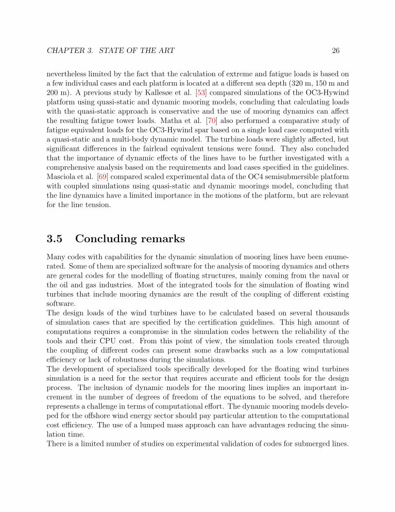
CHAPTER 3. STATE OF THE ART 26
nevertheless limited by the fact that the calculation of extreme and fatigue loads is based ona few individual cases and each platform is located at a different sea depth (320 m, 150 m and200 m). A previous study by Kallesøe et al. [53] compared simulations of the OC3-Hywindplatform using quasi-static and dynamic mooring models, concluding that calculating loadswith the quasi-static approach is conservative and the use of mooring dynamics can affectthe resulting fatigue tower loads. Matha et al. [70] also performed a comparative study offatigue equivalent loads for the OC3-Hywind spar based on a single load case computed witha quasi-static and a multi-body dynamic model. The turbine loads were slightly affected, butsignificant differences in the fairlead equivalent tensions were found. They also concludedthat the importance of dynamic effects of the lines have to be further investigated with acomprehensive analysis based on the requirements and load cases specified in the guidelines.Masciola et al. [69] compared scaled experimental data of the OC4 semisubmersible platformwith coupled simulations using quasi-static and dynamic moorings model, concluding thatthe line dynamics have a limited importance in the motions of the platform, but are relevantfor the line tension.
3.5 Concluding remarks
Many codes with capabilities for the dynamic simulation of mooring lines have been enume-rated. Some of them are specialized software for the analysis of mooring dynamics and othersare general codes for the modelling of floating structures, mainly coming from the naval orthe oil and gas industries. Most of the integrated tools for the simulation of floating windturbines that include mooring dynamics are the result of the coupling of different existingsoftware.The design loads of the wind turbines have to be calculated based on several thousandsof simulation cases that are specified by the certification guidelines. This high amount ofcomputations requires a compromise in the simulation codes between the reliability of thetools and their CPU cost. From this point of view, the simulation tools created throughthe coupling of different codes can present some drawbacks such as a low computationalefficiency or lack of robustness during the simulations.The development of specialized tools specifically developed for the floating wind turbinessimulation is a need for the sector that requires accurate and efficient tools for the designprocess. The inclusion of dynamic models for the mooring lines implies an important in-crement in the number of degrees of freedom of the equations to be solved, and thereforerepresents a challenge in terms of computational effort. The dynamic mooring models develo-ped for the offshore wind energy sector should pay particular attention to the computationalcost efficiency. The use of a lumped mass approach can have advantages reducing the simu-lation time.There is a limited number of studies on experimental validation of codes for submerged lines.

CHAPTER 3. STATE OF THE ART 27
All of them are based on the measurement of the tension of the line, but none has measuredthe motion of the line. The main disagreements with the lumped mass code predictions arereported in situations where the line looses the tension and suddenly recovers producing asnap load. This is a highly dynamic and challenging case that should be included in thevalidation of a mooring line code.The revision of the existing work on the influence of the mooring dynamics on the fatigue andultimate loads reveals that there is a lack of systematic and comprehensive studies. Existingworks have limitations and are based on a reduced number of simulation cases and platformmodels. The bibliographic sources point out the need of studies based on the methodologiesrequired by the certification standards.

28
Chapter 4
Dynamic simulation code for mooringlines
4.1 Abstract
In this chapter, the development of a dynamic computer code for the simulation of mooringlines is described. The code has been called OPASS (Offshore Platform Anchorage SystemSimulator). The basic system of equations that represents the dynamics of a line is deve-loped. These equations are discretized using the finite element method to obtain the setof equations implemented in the OPASS code. The mathematical model has been orientedto the achievement of a computationally efficient code. For this reason, a lumped mass ap-proach has been selected resulting in a global mass matrix composed of 3 x 3 submatrices inthe diagonal, that can be inverted with low computational cost. The code can be run as astandalone tool or coupled with FAST for the simulation of a complete floating wind turbine.
4.2 Basic dynamic equations
A mooring line has one of its ends fixed to the seabed by an anchor and the other end,called fairlead, is attached to the floating platform. The physical model considered in thiscode for the mooring is an slender line with constant circular section and three translationaldegrees of freedom at each node. Inertia, hydrodynamic added mass, gravity, hydrostatics,wave kinematics, tangential and normal hydrodynamic drag, axial elasticity and structuraldamping are considered. The code neglects the bending stiffness, being suitable for the si-mulation of chains. Part of the line can be in contact with the seabed and the line-seabedcontact and friction are included.A coordinate system l0 is defined in the line as the distance along the unstretched length ofthe line, from the anchor to the line section to be considered, as it is shown in Figure 4.1.
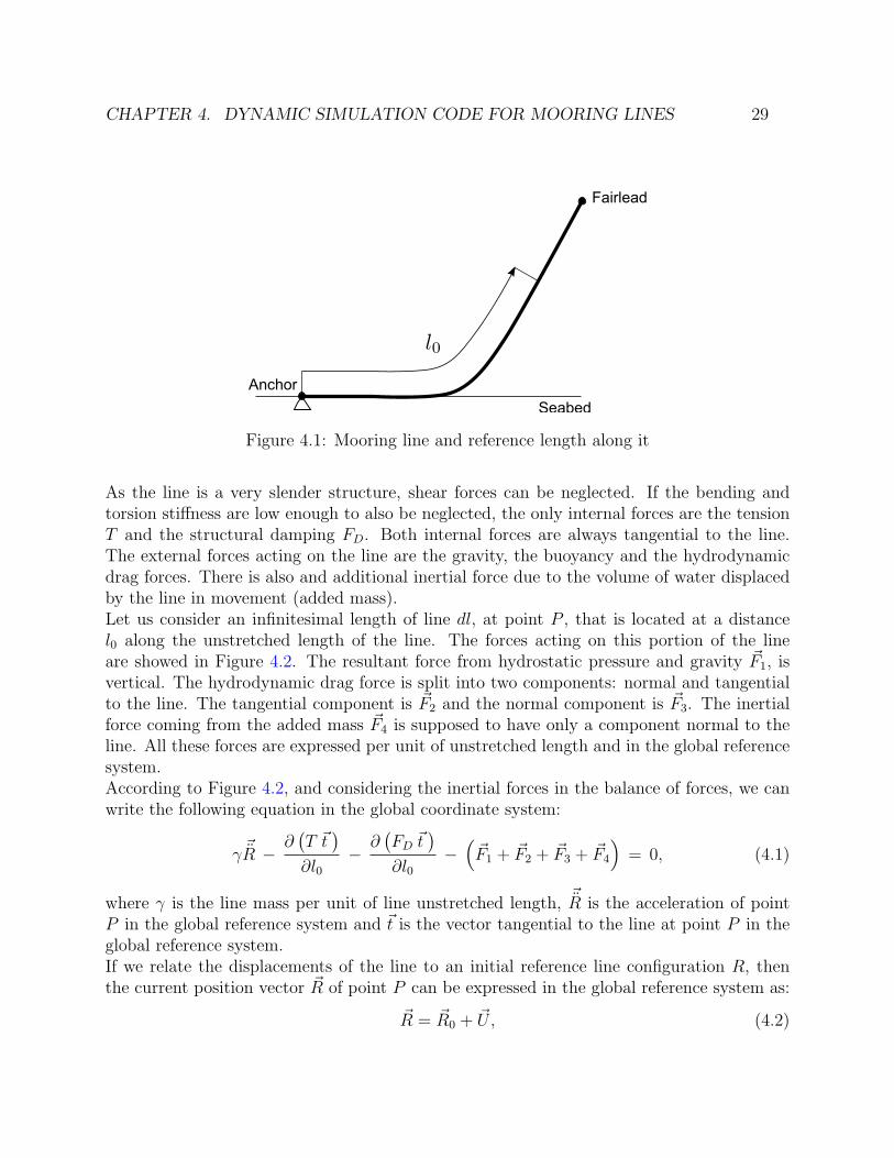
CHAPTER 4. DYNAMIC SIMULATION CODE FOR MOORING LINES 29
Seabed
Anchor
Fairlead
Figure 4.1: Mooring line and reference length along it
As the line is a very slender structure, shear forces can be neglected. If the bending andtorsion stiffness are low enough to also be neglected, the only internal forces are the tensionT and the structural damping FD. Both internal forces are always tangential to the line.The external forces acting on the line are the gravity, the buoyancy and the hydrodynamicdrag forces. There is also and additional inertial force due to the volume of water displacedby the line in movement (added mass).Let us consider an infinitesimal length of line dl, at point P , that is located at a distancel0 along the unstretched length of the line. The forces acting on this portion of the lineare showed in Figure 4.2. The resultant force from hydrostatic pressure and gravity F1, isvertical. The hydrodynamic drag force is split into two components: normal and tangentialto the line. The tangential component is F2 and the normal component is F3. The inertialforce coming from the added mass F4 is supposed to have only a component normal to theline. All these forces are expressed per unit of unstretched length and in the global referencesystem.According to Figure 4.2, and considering the inertial forces in the balance of forces, we canwrite the following equation in the global coordinate system:
γ R −∂(T t)
∂l0−∂(FD t
)∂l0
−(F1 + F2 + F3 + F4
)= 0, (4.1)
where γ is the line mass per unit of line unstretched length, R is the acceleration of pointP in the global reference system and t is the vector tangential to the line at point P in theglobal reference system.If we relate the displacements of the line to an initial reference line configuration R, thenthe current position vector R of point P can be expressed in the global reference system as:
R = R0 + U , (4.2)
CHAPTER 4. DYNAMIC SIMULATION CODE FOR MOORING LINES 30
Figure 4.2: Forces acting on an infinitesimal length of line
where R0 is the initial position vector of point P at the reference line configuration R, andU is the displacement vector. The vector tangential to the line at point P in Equation (4.1)can be calculated as:
t =∂R∂l0∣∣∂R∂l0
∣∣ (4.3)
4.2.1 Elastic forces
For the infinitesimal element that we are considering, the axial deformation ε is defined as:
ε =∂l
∂l0− 1 =
∣∣∣∣∂R∂l0∣∣∣∣− 1, (4.4)
where l is the distance along the stretched length of the line.The tension at point P can be obtained from the constitutive equation:
T = EAε, (4.5)
where E is the material Young’s modulus and A is the section area of the line.
4.2.2 Structural damping forces
The structural damping is based on the Rayleigh model (see, for example, [45]). In general,Rayleigh model assumes the damping to be proportional to the mass and the stiffness. Inthis model, the term proportional to the mass is neglected and the damping force FD atpoint P is considered only proportional to the stiffness EA as it is commonly assumed inthe modelling of mooring lines for integrated codes [64], [87]. The proportionality coefficientis β. Thus, we can formulate:
FD = βEA ε, (4.6)
where ε is the deformation velocity.
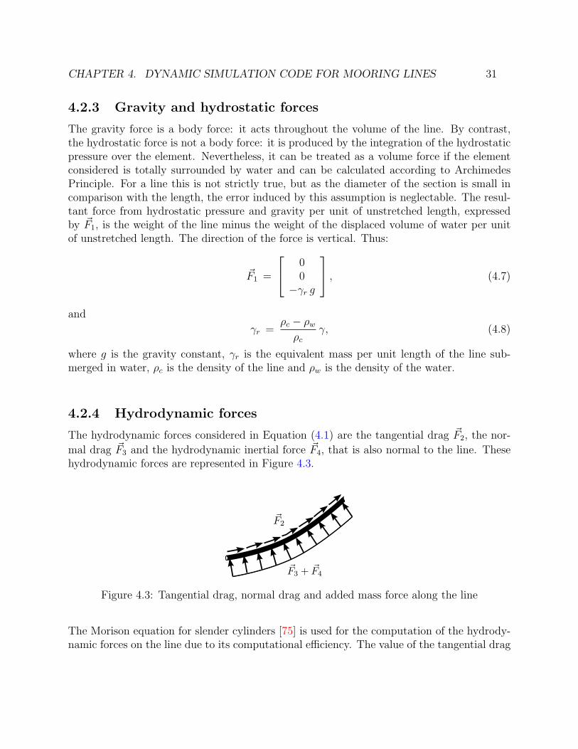
CHAPTER 4. DYNAMIC SIMULATION CODE FOR MOORING LINES 31
4.2.3 Gravity and hydrostatic forces
The gravity force is a body force: it acts throughout the volume of the line. By contrast,the hydrostatic force is not a body force: it is produced by the integration of the hydrostaticpressure over the element. Nevertheless, it can be treated as a volume force if the elementconsidered is totally surrounded by water and can be calculated according to ArchimedesPrinciple. For a line this is not strictly true, but as the diameter of the section is small incomparison with the length, the error induced by this assumption is neglectable. The resul-tant force from hydrostatic pressure and gravity per unit of unstretched length, expressedby F1, is the weight of the line minus the weight of the displaced volume of water per unitof unstretched length. The direction of the force is vertical. Thus:
F1 =
00
−γr g
, (4.7)
and
γr =ρc − ρwρc
γ, (4.8)
where g is the gravity constant, γr is the equivalent mass per unit length of the line sub-merged in water, ρc is the density of the line and ρw is the density of the water.
4.2.4 Hydrodynamic forces
The hydrodynamic forces considered in Equation (4.1) are the tangential drag F2, the nor-
mal drag F3 and the hydrodynamic inertial force F4, that is also normal to the line. Thesehydrodynamic forces are represented in Figure 4.3.
Figure 4.3: Tangential drag, normal drag and added mass force along the line
The Morison equation for slender cylinders [75] is used for the computation of the hydrody-namic forces on the line due to its computational efficiency. The value of the tangential drag

CHAPTER 4. DYNAMIC SIMULATION CODE FOR MOORING LINES 32
force per unit length of the unstretched line can be calculated as:
F2 = C2|Vt|Vt(1 + ε) = C2
(∣∣V · t∣∣ V · t
)(1 + ε) t,
C2 = 12CdtDρw,
(4.9)
where Cdt is the tangential drag coefficient and D is the diameter of the line. The vector Vis the relative velocity between the water and the line and Vt is the component tangential tothe element, both expressed in the global reference system.In a similar way, the drag force normal to the line per unit length can be obtained :
F3 = C3|Vn|Vn (1 + ε) = C3
[V · V −
(V · t
)2] 12 [V −
(V · t
)t](1 + ε),
C3 =1
2CdnDρw,
(4.10)
where Cdn is the normal drag coefficient and Vn is the component normal to the element ofthe relative velocity between the water and the line.The hydrodynamic inertial force per unit of unstretched line length is calculated based on anormal added mass coefficient Cmn as:
F4 = −C4 (1 + ε)[R− ( R · t ) t
]C4 = Cmn
πD2
4ρw
(4.11)
Substituting Equations (4.5), (4.6) and (4.11) into (4.1) finally results in:
γ R + C4 (1 + ε)[R− ( R · t ) t
]− ∂(EAε t )
∂l0− ∂(βEA ε t)
∂l0− F1 − F2 − F3 = 0 (4.12)
4.3 The finite element equations
4.3.1 Virtual Works principle
According to the Virtual Works Principle, if we apply a small (virtual) displacement that
satisfies the boundary conditions, δU , with respect to a certain equilibrium configuration ofthe line at time t, the virtual work WV done by the external and internal forces along theline length must be zero. The virtual work can be obtained by multiplying Equation (4.12)
by the virtual displacement δU and integrating along the line length:
WV =
∫ L
0
{(γ R + C4(1 + ε)
[R− ( R · t ) t
])· δU −
(F1 + F2 + F3
)· δU+
+EAε∂δU
∂l0· t+ βEA ε
∂δU
∂l0· t
}dl0 − [EAεt · δU ] L0 − [βEA εt · δU ] L0 = 0,
(4.13)
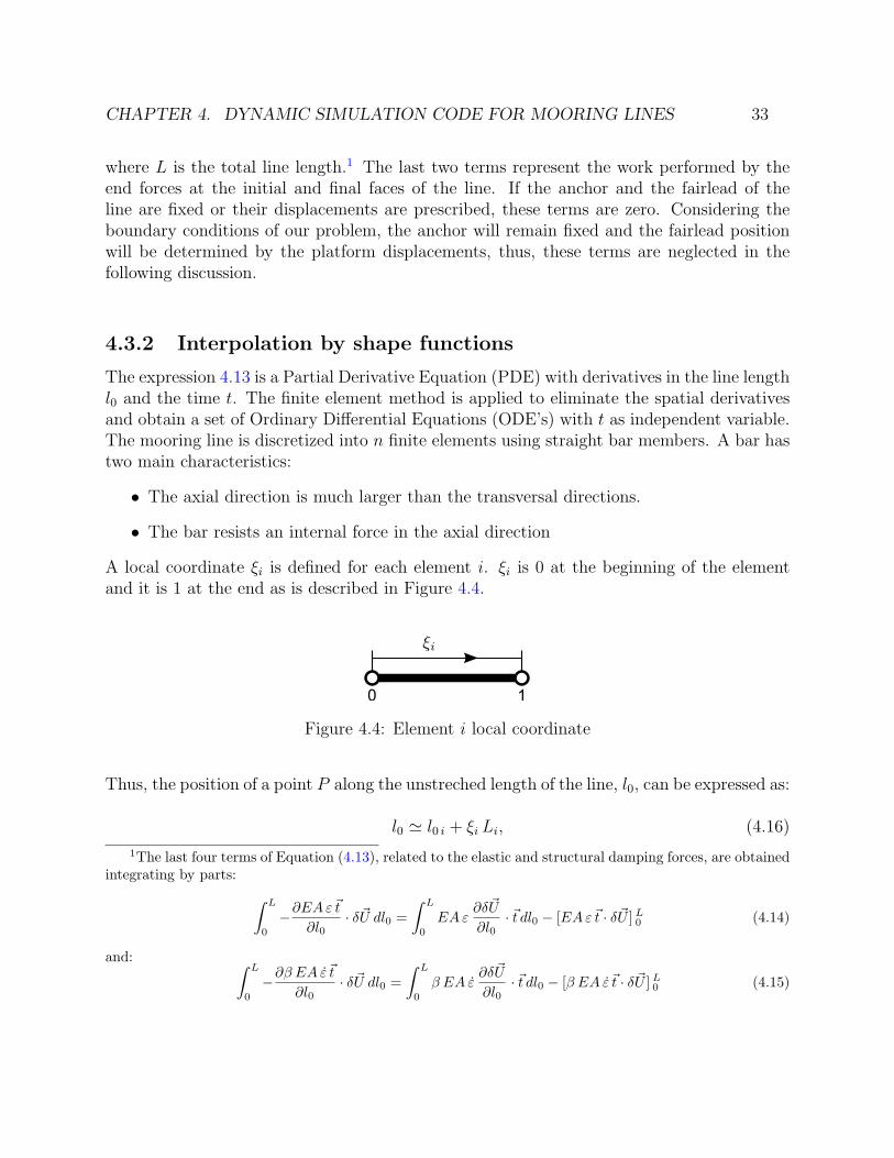
CHAPTER 4. DYNAMIC SIMULATION CODE FOR MOORING LINES 33
where L is the total line length.1 The last two terms represent the work performed by theend forces at the initial and final faces of the line. If the anchor and the fairlead of theline are fixed or their displacements are prescribed, these terms are zero. Considering theboundary conditions of our problem, the anchor will remain fixed and the fairlead positionwill be determined by the platform displacements, thus, these terms are neglected in thefollowing discussion.
4.3.2 Interpolation by shape functions
The expression 4.13 is a Partial Derivative Equation (PDE) with derivatives in the line lengthl0 and the time t. The finite element method is applied to eliminate the spatial derivativesand obtain a set of Ordinary Differential Equations (ODE’s) with t as independent variable.The mooring line is discretized into n finite elements using straight bar members. A bar hastwo main characteristics:
• The axial direction is much larger than the transversal directions.
• The bar resists an internal force in the axial direction
A local coordinate ξi is defined for each element i. ξi is 0 at the beginning of the elementand it is 1 at the end as is described in Figure 4.4.
0 1
Figure 4.4: Element i local coordinate
Thus, the position of a point P along the unstreched length of the line, l0, can be expressed as:
l0 ≃ l0 i + ξi Li, (4.16)
1The last four terms of Equation (4.13), related to the elastic and structural damping forces, are obtainedintegrating by parts: ∫ L
0
−∂EAε t
∂l0· δU dl0 =
∫ L
0
EAε∂δU
∂l0· t dl0 − [EAε t · δU ] L0 (4.14)
and: ∫ L
0
−∂β EA ε t
∂l0· δU dl0 =
∫ L
0
β EA ε∂δU
∂l0· t dl0 − [β EA ε t · δU ] L0 (4.15)
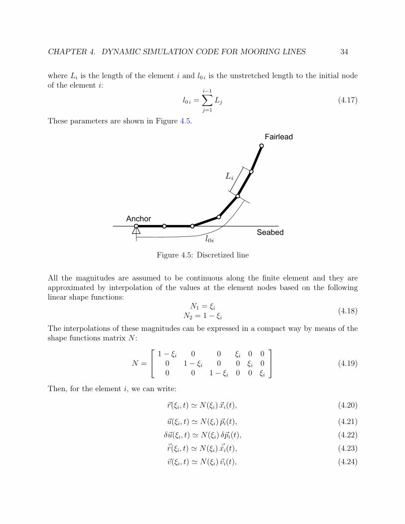
CHAPTER 4. DYNAMIC SIMULATION CODE FOR MOORING LINES 34
where Li is the length of the element i and l0 i is the unstretched length to the initial nodeof the element i:
l0 i =i−1∑j=1
Lj (4.17)
These parameters are shown in Figure 4.5.
Seabed
Anchor
Fairlead
Figure 4.5: Discretized line
All the magnitudes are assumed to be continuous along the finite element and they areapproximated by interpolation of the values at the element nodes based on the followinglinear shape functions:
N1 = ξiN2 = 1− ξi
(4.18)
The interpolations of these magnitudes can be expressed in a compact way by means of theshape functions matrix N :
N =
1− ξi 0 0 ξi 0 00 1− ξi 0 0 ξi 00 0 1− ξi 0 0 ξi
(4.19)
Then, for the element i, we can write:
r(ξi, t) ≃ N(ξi) xi(t), (4.20)
u(ξi, t) ≃ N(ξi) pi(t), (4.21)
δu(ξi, t) ≃ N(ξi) δpi(t), (4.22)
r(ξi, t) ≃ N(ξi) xi(t), (4.23)
v(ξi, t) ≃ N(ξi) vi(t), (4.24)

CHAPTER 4. DYNAMIC SIMULATION CODE FOR MOORING LINES 35
where r and r are the 3 x 1 position and velocity vectors in the element reference system andxi and xi are the 6 x 1 element nodal position and element nodal velocity vectors, both inthe element reference system. The vectors u and δu are the 3 x 1 displacement and virtualdisplacement vectors and pi and δpi are the respective 6 x 1 element i nodal displacement andelement i nodal virtual displacement vectors, all in the element reference system. Finally, vis the relative velocity of the water and vi is the element i nodal vector for the relative watervelocity in the local reference system.For the inertial forces, instead of linear shape functions, discontinuous step functions aredefined, resulting on a lumped mass model. The resulting global mass matrix is composed of3 x 3 submatrices located at the diagonal. This is an important advantage for the inversionof the matrix that can be done with much less computational effort.
N ′ =
ψ1 0 0 ψ2 0 00 ψ1 0 0 ψ2 00 0 ψ1 0 0 ψ2
, (4.25)
where:
ψ1 = 1ψ2 = 0
}ξi ∈ [0, 0.5]
ψ1 = 0ψ2 = 1
}ξi ∈ [0.5, 1]
(4.26)
So, the accelerations within element i are approximated as:
r(ξi, t) ≃ N ′(ξi) xi(t), (4.27)
where r is the acceleration vector and xi is the 6 x 1 element vector with the nodal accele-rations, both in the local element system.Finally, the matrix B is defined as the derivative of N :
B =∂N
∂ξi=
−1 0 0 1 0 00 −1 0 0 1 00 0 −1 0 0 1
(4.28)
4.3.3 Local to global transformation matrix
The magnitudes in the local reference system of the i element and in the global referencesystem can be related through the 3 x 3 local to global transformation matrix Ti. To findthe unit direction vectors, e1i, e2i and e3i, that compose the local reference system attachedto the bar element i, together with the element initial node (node 1) and final node (node2), an additional node has to be defined. The position of this third node is arbitrary, thoughit has to be located out of the element, to define the plane containing the e2i unit vector.
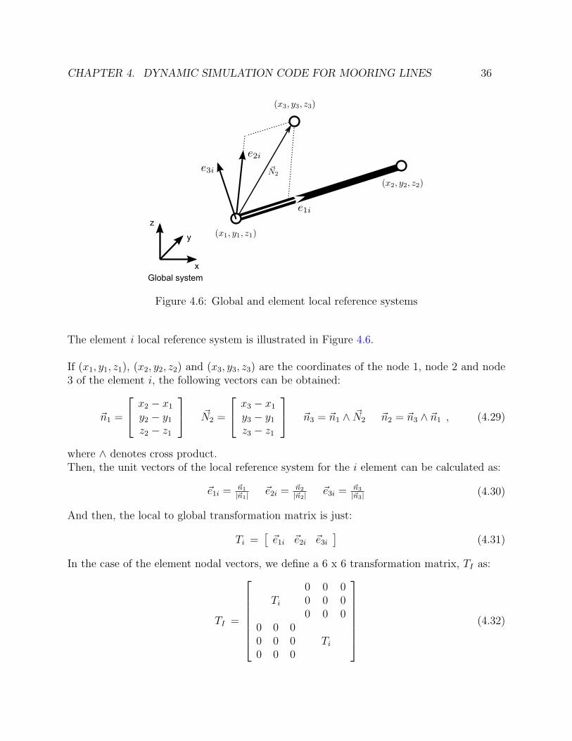
CHAPTER 4. DYNAMIC SIMULATION CODE FOR MOORING LINES 36
x
y
z
Global system
Figure 4.6: Global and element local reference systems
The element i local reference system is illustrated in Figure 4.6.
If (x1, y1, z1), (x2, y2, z2) and (x3, y3, z3) are the coordinates of the node 1, node 2 and node3 of the element i, the following vectors can be obtained:
n1 =
x2 − x1y2 − y1z2 − z1
N2 =
x3 − x1y3 − y1z3 − z1
n3 = n1 ∧ N2 n2 = n3 ∧ n1 , (4.29)
where ∧ denotes cross product.Then, the unit vectors of the local reference system for the i element can be calculated as:
e1i =n1
|n1| e2i =n2
|n2| e3i =n3
|n3| (4.30)
And then, the local to global transformation matrix is just:
Ti =[e1i e2i e3i
](4.31)
In the case of the element nodal vectors, we define a 6 x 6 transformation matrix, TI as:
TI =
0 0 0
Ti 0 0 00 0 0
0 0 00 0 0 Ti0 0 0
(4.32)

CHAPTER 4. DYNAMIC SIMULATION CODE FOR MOORING LINES 37
The matrices N and N ′ interpolate the nodal magnitudes in the element local referencesystem. By means of the transformation matrices, we can define new matrices Ng i, N
′g i and
Bg i to operate with the magnitudes at element i in the global system:
Ng i = TiNTTI (4.33)
N ′g i = TiN
′T TI (4.34)
Bg i = TiBTTI (4.35)
Thus:R(ξi, t) ≃ Ng i(ξi) Xi(t) (4.36)
U(ξi, t) ≃ Ng i(ξi) Pi(t) (4.37)
δU(ξi, t) ≃ Ng i(ξi) δPi(t) (4.38)
R(ξi, t) ≃ Ng i(ξi)Xi(t) (4.39)
R(ξi, t) ≃ N ′g i(ξi)
Xi(t) (4.40)
V (ξi, t) ≃ Ng i(ξi) Vi(t) (4.41)
Where R is the 3 x 1 velocity vector, and Xi,Xi and Xi are the 6 x 1 element i nodal
position, velocity and acceleration vectors, all in the global reference system. Pi and δPi arethe element nodal displacement and virtual displacement vectors, also in the global system.Finally, Vi is the element nodal relative water velocity in the global reference system.
4.3.4 Definition of the adjacency matrix
We define for each element i an adjacency matrix Ai, composed of elements with value 0or 1, that relates the 6 x 1 element i nodal vectors with the whole 6(n+1) x 1 discretizedsystem global vector. So, the dimension of Ai is 6 x 6(n+1). If the nodes are numberedconsecutively, then the adjacency matrix of the element i has the following structure:
0 0 1 0 0 0 0 0 0 00 0 0 1 0 0 0 0 0 00 ... 0 0 0 1 0 0 0 0 ... 00 0 0 0 0 1 0 0 0 00 0 0 0 0 0 1 0 0 00 0 0 0 0 0 0 1 0 0
Index : 1 ... i− 1 i i+ 2 i+ 3 i+ 4 i+ 5 i+ 6 i+ 7 ... 6n+ 6
(4.42)

CHAPTER 4. DYNAMIC SIMULATION CODE FOR MOORING LINES 38
And then:Xi = AiX (4.43)
Xi = AiX (4.44)
Xi = AiX (4.45)
δPi = AiδP (4.46)
This is a mathematical way to express the assembly of the discretized matrices implementedin the code.
4.3.5 Discretization of elastic forces
As we have neglected the elastic forces acting at the end sections of the line, the term forthe work produced by the elastic forces Welastic in Equation (4.13) is:
Welastic =
∫ L
0
EAε∂δU
∂l0· t dl0 (4.47)
The discretized element deformation εi is obtained deriving the expression (4.36) and intro-ducing it into Equation (4.4):
ε =
∣∣∣∣∂R∂l0∣∣∣∣− 1 ≃ εi =
√Bg iXi
Li
· Bg iXi
Li
− 1 =
√XT
i BTg iBg iXi
Li
− 1
i−1∑j=1
jLj < l0 ≤i∑
j=1
jLj
(4.48)
On the other hand, from derivation of Equation (4.38) we have:
∂δU
∂l0≃ Bg i
δPi
Li
i−1∑j=1
jLj < l0 ≤i∑
j=1
jLj (4.49)
And the tangential vector t can be expressed introducing into (4.3) the derivative of theexpression (4.36):
t =∂R∂l0∣∣∂R∂l0
∣∣ ≃ Bg i Xi∣∣Bg i Xi
∣∣ =Bg i Xi
Li (1 + εi)
i−1∑j=1
jLj < l0 ≤i∑
j=1
jLj (4.50)
Introducing into (4.47) the expressions (4.43), (4.46), (4.49) and (4.50), we have:
Welastic ≃n∑
i=1
∫ 1
0
EAεiδP TAT
i BTg iBg iAiX
Li (1 + εi)dξ (4.51)
CHAPTER 4. DYNAMIC SIMULATION CODE FOR MOORING LINES 39
4.3.6 Discretization of structural damping forces
The term in Equation (4.13) for the work produced by the structural damping forces Wdamp
is:
Wdamp =
∫ L
0
βEA ε∂δU
∂l0· t dl0 (4.52)
The element deformation velocity can be obtained by the time derivation of the expression(4.48):
ε ≃ εi =dεidt
=XT
i BTg iBg i
Xi
L2i (1 + εi)
i−1∑j=1
jLj < l0 ≤i∑
j=1
jLj (4.53)
If we follow a parallel reasoning as to discretize the work of the elastic forces, we obtain thefollowing expression:
Wdamp ≃n∑
i=1
∫ 1
0
βEA εiδP TAT
i BTg iBg i Xi
Li (1 + εi)dξ (4.54)
And using (4.44) and (4.53), we have:
Wdamp =n∑
i=1
∫ 1
0
βEAδP TAT
i BTg iBg i XiX
Ti B
Tg iBg iAi
X
L3i (1 + εi)
2 dξ (4.55)
4.3.7 Discretization of external forces
The external forces considered are the gravity and the buoyancy F1, the tangential hy-drodynamic force F2 and the normal hydrodynamic drag F3. The force produced by thehydrodynamic added mass is studied separately, as an inertial force.Thus, the work due to these external forces in Equation (4.13), Wexternal, is:
Wexternal =
∫ L
0
−(F1 + F2 + F3
)· δU dl0 (4.56)
The discretization of the distributed external forces F1, F2 and F3 respectively results in theresultant gravity and buoyancy elemental force: F1 i; the tangential drag elemental force:F2 i and the normal drag elemental force: F3 i.The expression for F1 i can be easily obtained since F1 is constant and does not depend onthe element local coordinate ξ. Thus, the discretized gravity and buoyancy force for theelement i is just:
F1 ≃ F1 i =
0−γr g0
(4.57)
CHAPTER 4. DYNAMIC SIMULATION CODE FOR MOORING LINES 40
F2 i is calculated from expression (4.9), using (4.41) and (4.50):
F2 ≃ F2 i =C2
L3i (1 + εi)2
∣∣V Ti N
Tg iBg iXi
∣∣ (V Ti N
Tg iBg iXi
)Bg iXi
i−1∑j=1
jLj < l0 ≤i∑
j=1
jLj
(4.58)
And in the same way, F3 i is obtained introducing (4.41) and (4.50) in the expression (4.10):
F3 ≃ F3 i = C3(1 + εi)
V Ti N
Tg iNg iVi −
(V Ti N
Tg iBg iXi
)2(1 + εi)2L2
i
12
Ng iVi −
(V Ti N
Tg iBg iXi
)Bg iXi
(1 + εi)2L2i
i−1∑j=1
jLj < l0 ≤i∑
j=1
jLj
(4.59)
Including into (4.56) the expressions (4.38), (4.46), (4.57), (4.58) and (4.57) we have:
Wexternal ≃i−1∑j=1
∫ 1
0
−δP TATi N
Tg i
(F1 i + F2 i + F3 i
)Lidξ (4.60)
4.3.8 Discretization of inertial forces
Finally, the term for the work produced by the inertial forces Winertial in Equation (4.13) is:
Winertia =
∫ L
0
(γ R + C4(1 + ε)
[R− ( R · t ) t
])· δUdl0 (4.61)
If we substitute into (4.61) the expressions (4.38), (4.40), (4.45), (4.46) and (4.50), we have:
Winertia ≃i−1∑j=1
∫ 1
0
δP Ti A
Ti N
′ Tg i
(γ LiN
′g iAi + C4
[Li(1 + εi)N
′g iAi−
−Bg iXiXi
TBT
g iN′g iAi
Li (1 + εi)
Xdξ
(4.62)
4.3.9 Discretized equations of motion
Once we have obtained the discretized expressions for the different terms of work within theEquation (4.13) (Equations (4.51), (4.54), (4.60) and (4.62) ), we can built the following
CHAPTER 4. DYNAMIC SIMULATION CODE FOR MOORING LINES 41
equation for the total virtual work:
WV ≃ δP T
n∑i=1
∫ 1
0
(γ LiA
Ti N
′ Tg i N
′g iAi
X + C4
[Li(1 + εi)A
Ti N
′ Tg i N
′g iAi−
−AT
i N′ Tg i Bg iXiX
Ti B
Tg iN
′g iAi
Li (1 + εi)
]X − LiA
Ti N
Tg i
(F1 i + F2 i + F3 i
)+
+βEAAT
i BTg iBg i XiX
Ti B
Tg iBg iAi
L3i (1 + εi)
2X + EAεi
ATi B
Tg iBg iAi
Li (1 + εi)X
)dξ = 0
(4.63)
The virtual displacement δP can be eliminated from the expression (4.63) since it is anarbitrary displacement. This allow us to finally find the equations of motion of the systemin the following form:
M X + C X +K X − F = 0, (4.64)
where M is the mass matrix of the system:
M =n∑
i=1
ATi
∫ 1
0
(γ LiN
′ Tg i N
′g i + C4
[Li(1 + εi)N
′ Tg i N
′g i−
−N
′ Tg i Bg iXiX
Ti B
Tg iN
′g i
Li (1 + εi)
])dξi Ai
(4.65)
C is the structural damping matrix of the system:
C =n∑
i=1
ATi
∫ 1
0
βEABT
g iBg i Xi XTi B
Tg iBg i
L3i (1 + εi)
2 dξi Ai (4.66)
The stiffness matrix of the system, K is:
K =n∑
i=1
ATi
∫ 1
0
EAεiBT
g iBg i
Li (1 + εi)dξi Ai (4.67)
And F are the external forces of the discretized system:
F =n∑
i=1
ATi
∫ 1
0
LiNTg i
(F1 i + F2 i + F3 i
)dξi (4.68)
4.3.10 Elemental matrices and force vectors
The Equations (4.65), (4.66), (4.67) and (4.68) provide the expressions to build the massmatrix, the structural damping matrix, the stiffness matrix and the external force vector of
CHAPTER 4. DYNAMIC SIMULATION CODE FOR MOORING LINES 42
the complete system in the global reference system. These global matrices and vectors arethe result of the assembly of the elemental matrices and forces. This assembly procedure isexpressed mathematically by the products with the adjacency matrix Ai.It is trivial to derive from these equations the expressions for the elemental mass matrix Mi,the structural damping matrix Ci, the structural stiffness matrix Ki and the force vector Fi
in the global reference system:
Mi =
∫ 1
0
(γ LiN
′ Tg i N
′g i + C4
[Li(1 + εi)N
′ Tg i N
′g i −
N′ Tg i Bg iXiX
Ti B
Tg iN
′g i
Li (1 + εi)
])dξi (4.69)
Ci =
∫ 1
0
βEABT
g iBg i Xi XTi B
Tg iBg i
L3i (1 + εi)
2 dξi (4.70)
Ki =
∫ 1
0
EAεiBT
g iBg i
Li (1 + εi)dξi (4.71)
Fi =
∫ 1
0
LiNTg i
(F1 i + F2 i + F3 i
)dξi (4.72)
These elemental matrices and forces can also be expressed in the elemental reference system:
mi =
∫ 1
0
(γ LiN
′ TN ′ + C4
[Li(1 + εi)N
′ TN ′ − N′ TBXiX
Ti B
TN ′
Li (1 + εi)
])dξi (4.73)
ci =
∫ 1
0
βEABT B Xi X
Ti B
TB
L3i (1 + εi)
2 dξi (4.74)
ki =
∫ 1
0
EAεiBT B
Li (1 + εi)dξi (4.75)
fi =
∫ 1
0
LiNT(f1 i + f2 i + f3 i
)dξi, (4.76)
where:
f1 i = T Ti
0−γr g0
(4.77)

CHAPTER 4. DYNAMIC SIMULATION CODE FOR MOORING LINES 43
f2 i =C2
L3i (1 + εi)2
∣∣vTi NTBxi∣∣ (vTi NTBxi
)Bxi (4.78)
f3 i = C3(1 + εi)
[vTi N
TNvi −(vTi N
TBxi)2
(1 + εi)2L2i
] 12[Nvi −
(vTi N
TBxi)Bxi
(1 + εi)2L2i
](4.79)
4.4 Code implementation of the mooring lines
dynamics
A computer program in Fortran 90 based on the theoretical development described in Section4.3, has been developed with the capability of simulating the dynamics of a mooring linesubmerged in water, under the action of waves and in contact with the seabed. The codehas been named OPASS (”Offshore Platform Anchorage System Simulator”).
4.4.1 Implementation of the finite element method
The equation of motion of the system (4.64) is built according to the classical steps of thefinite element method:
1. Discretize the line in a finite number of bar elements.
2. Built the elemental mass, damping and stiffness matrices using Equations (4.73), (4.74),(4.75) and the external force vectors according to (4.76).
3. Transform the elemental matrices and force vectors into the global coordinate systemusing the local to global transformation matrix (4.32).
4. Assembly the global mass, damping and stiffness matrices and the global externalforces vector using the adjacency matrices (4.42).
The resultant system of equations of motion are ordinary differential equations.Alternatively, the steps 2 and 3 can be performed in only one step using the Equations(4.69), (4.70), (4.71) and (4.72). These are the expressions that have been implemented inthe code, providing a better computational efficiency.As has been explained in Subsection 4.3.2, the interpolation function chosen for the inertialforces are step functions instead of linear functions. This results in a mass matrix composedof 3 x 3 submatrices around the diagonal. Thus, the assembly of the matrices and forcevector (step 4) can be simplified and the inversion of the mass matrix is performed withmuch lower computational cost.The efficiency in the computation of the matrices and also in the inversion of the mass matrixis important to obtain a fast simulation code, because matrices are calculated at every time
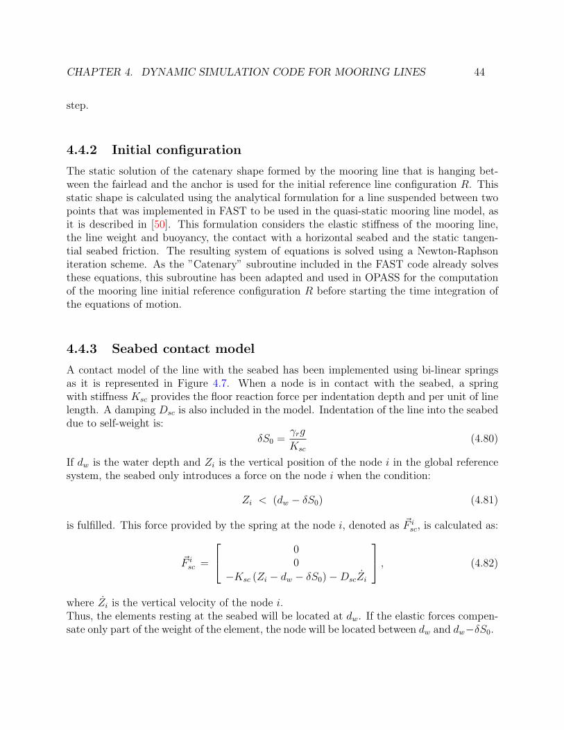
CHAPTER 4. DYNAMIC SIMULATION CODE FOR MOORING LINES 44
step.
4.4.2 Initial configuration
The static solution of the catenary shape formed by the mooring line that is hanging bet-ween the fairlead and the anchor is used for the initial reference line configuration R. Thisstatic shape is calculated using the analytical formulation for a line suspended between twopoints that was implemented in FAST to be used in the quasi-static mooring line model, asit is described in [50]. This formulation considers the elastic stiffness of the mooring line,the line weight and buoyancy, the contact with a horizontal seabed and the static tangen-tial seabed friction. The resulting system of equations is solved using a Newton-Raphsoniteration scheme. As the ”Catenary” subroutine included in the FAST code already solvesthese equations, this subroutine has been adapted and used in OPASS for the computationof the mooring line initial reference configuration R before starting the time integration ofthe equations of motion.
4.4.3 Seabed contact model
A contact model of the line with the seabed has been implemented using bi-linear springsas it is represented in Figure 4.7. When a node is in contact with the seabed, a springwith stiffness Ksc provides the floor reaction force per indentation depth and per unit of linelength. A damping Dsc is also included in the model. Indentation of the line into the seabeddue to self-weight is:
δS0 =γrg
Ksc
(4.80)
If dw is the water depth and Zi is the vertical position of the node i in the global referencesystem, the seabed only introduces a force on the node i when the condition:
Zi < (dw − δS0) (4.81)
is fulfilled. This force provided by the spring at the node i, denoted as F isc, is calculated as:
F isc =
00
−Ksc (Zi − dw − δS0)−DscZi
, (4.82)
where Zi is the vertical velocity of the node i.Thus, the elements resting at the seabed will be located at dw. If the elastic forces compen-sate only part of the weight of the element, the node will be located between dw and dw−δS0.
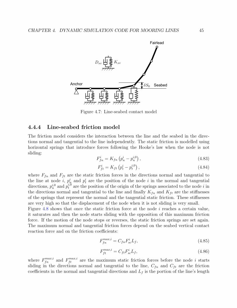
CHAPTER 4. DYNAMIC SIMULATION CODE FOR MOORING LINES 45
Anchor Seabed
Fairlead
Figure 4.7: Line-seabed contact model
4.4.4 Line-seabed friction model
The friction model considers the interaction between the line and the seabed in the direc-tions normal and tangential to the line independently. The static friction is modelled usinghorizontal springs that introduce forces following the Hooke’s law when the node is notsliding:
F ifn = Kfn
(pin − pi,0n
), (4.83)
F ift = Kft
(pit − pi,0t
), (4.84)
where Ffn and Fft are the static friction forces in the directions normal and tangential tothe line at node i, pin and pit are the position of the node i in the normal and tangentialdirections, pi,0n and pi,0t are the position of the origin of the springs associated to the node i inthe directions normal and tangential to the line and finally Kfn and Kft are the stiffnessesof the springs that represent the normal and the tangential static friction. These stiffnessesare very high so that the displacement of the node when it is not sliding is very small.Figure 4.8 shows that once the static friction force at the node i reaches a certain value,it saturates and then the node starts sliding with the opposition of this maximum frictionforce. If the motion of the node stops or reverses, the static friction springs are set again.The maximum normal and tangential friction forces depend on the seabed vertical contactreaction force and on the friction coefficients:
Fmax,ifn = CfnF
iscLf , (4.85)
Fmax,ift = CftF
iscLf , (4.86)
where Fmax,ifn and Fmax,i
ft are the maximum static friction forces before the node i startssliding in the directions normal and tangential to the line, Cfn and Cft are the frictioncoefficients in the normal and tangential directions and Lf is the portion of the line’s length

CHAPTER 4. DYNAMIC SIMULATION CODE FOR MOORING LINES 46
that is represented by the node i for the computation of the friction forces.
Figure 4.8: Friction model implemented in all the nodes in contact with the seabed in thedirections normal and tangential to the line
4.4.5 Time integration of the equations
The system of equations (4.64) that we have obtained through the finite element methodcan be rewritten as:
X =M−1(F − C X −K X
)(4.87)
To integrate this equation in time, three different integration schemes were implemented.The first one is a simple explicit scheme described in [63] and [64], based on the centraldifference formula.The second integrator is the Runge-Kutta-Nystrom scheme described in [42]. This methodrequires four evaluations of the equations of the lines (4.87) per time step, increasing thecomputational effort, but, on the other hand, it allows to increase the size of the time step.Finally, the third integrator is the Adams-Moulton-Bashforth predictor-corrector scheme[31], where the solution at each time step is achieved by evaluating twice the equations ofmotion (4.87). In the first evaluation, called predictor stage, the accelerations are obtainedfrom the equations of motion of the system and they are used to calculate the positions andvelocities of the line’s degrees of freedom at the next time step. In a second stage, calledcorrector, this solution is refined using the next time step positions and velocities to obtainmore accurate accelerations for the next step. A final estimation of positions and velocitiesfrom these accelerations is performed and one time step is advanced.

CHAPTER 4. DYNAMIC SIMULATION CODE FOR MOORING LINES 47
4.5 Verification of the OPASS code
The OPASS code has been successfully verified against computations with the 3DFloat code[22], [12], [11].In addition, OPASS has been coupled with the FAST code [50], whose original FAST mooringlines model is a quasi-static approach, expanding its capabilities for the integrated simula-tion of floating offshore wind turbines. A verification of OPASS coupled with FAST wassatisfactorily carried out within the IEA Annex 30 benchmark (OC4) [88], [9]. This coupledversion will be used in the research carried out in Chapter 6.
4.6 Concluding remarks
The equations of motion of a submerged line are set and solved using a FEM technique. Alumped mass formulation oriented to achieve high computational efficiency has been adopted.The global mass matrix is composed of 3 x 3 submatrices in the diagonal resulting in easilyinvertible matrix with low CPU cost. The code has been verified against computations withother existing tools for mooring lines and also, coupled with FAST, by taking part in theIEA Annex 30 (OC4) international simulation codes benchmark.

48
Chapter 5
Experimental validation of the code
5.1 Abstract
In this chapter, the OPASS numerical simulation code developed in Chapter 4 is experimen-tally validated against a set of tests performed at the Ecole Centrale de Nantes (ECN) wavetank in France. The tests consist of a suspended chain submerged into a water basin, wherethe suspension point of the chain is excited with horizontal harmonic motions of differentperiods in the plane of the catenary. Equivalent simulations of the chain setup are launchedto compare against the experimental results. The description of the tests, the results and theconclusions presented in this chapter have been published in [10] and [8]. The code is ableto predict the tension at the suspension point and the motions at several positions of theline with high accuracy. Even for those cases where the line loses and subsequently recoverstension, the resulting snap load and motions are well captured with a slight overpredictionof the maximum tension. The drag coefficients for chains used in the computations havebeen taken from the DNV guidelines and, in general, predict correctly the hydrodynamicloads. In addition, sensitivity studies and verification against another code show that highlydynamic cases are sensitive to the seabed-cable contact and friction models. The resultsshow the importance of capturing the evolution of the mooring dynamics for the predictionof the line tension, especially for the high frequency motions.
5.2 Description of the experiments
The dimensions of the Ecole Centrale de Nantes wave tank are 50m length, 30m width and5m depth. The chain was submerged into the water basin, forming a catenary shape with thebottom end anchored to the tank floor. The suspension point was connected through a loadcell to a mechanical actuator with the capability of reproducing a prescribed motion thatwas located at the water free surface. Figure 5.1 shows the configuration of the experiment.The fairlead, located at the water plane, was excited by the mechanical actuator with a si-
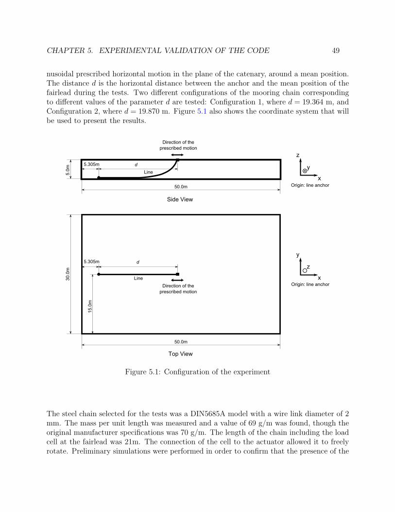
CHAPTER 5. EXPERIMENTAL VALIDATION OF THE CODE 49
nusoidal prescribed horizontal motion in the plane of the catenary, around a mean position.The distance d is the horizontal distance between the anchor and the mean position of thefairlead during the tests. Two different configurations of the mooring chain correspondingto different values of the parameter d are tested: Configuration 1, where d = 19.364 m, andConfiguration 2, where d = 19.870 m. Figure 5.1 also shows the coordinate system that willbe used to present the results.
Direction of the
prescribed motion
d
Line
50.0m
30.0
m
x
z
y
Origin: line anchor
15.0
m
5.305m
Top View
d
Line
50.0m
5.0
m
x
y
z
Origin: line anchor
5.305m
Side View
Direction of the
prescribed motion
Figure 5.1: Configuration of the experiment
The steel chain selected for the tests was a DIN5685A model with a wire link diameter of 2mm. The mass per unit length was measured and a value of 69 g/m was found, though theoriginal manufacturer specifications was 70 g/m. The length of the chain including the loadcell at the fairlead was 21m. The connection of the cell to the actuator allowed it to freelyrotate. Preliminary simulations were performed in order to confirm that the presence of the
CHAPTER 5. EXPERIMENTAL VALIDATION OF THE CODE 50
load cell has not an important impact on the dynamics of the chain. It was confirmed thatit has a neglectable impact on the computed tensions.This chain model was chosen because if a scale factor of 1/40 is considered, the 5 m depth ofthe basin represents a 200m depth sea location, and the resulting chain full scale propertiesare close to the OC4 floating model mooring lines [87]. Therefore, this chain represents atypical scaled mooring line used in wave tank tests for floating wind turbines.First, two static cases with the chain suspension point fixed corresponding to Configuration1 and Configuration 2 were studied. In addition, 6 dynamic cases were simulated combiningthe 2 chain configurations with three different oscillation periods of the motion imposed atthe fairlead. Similar criteria based on scale factors used for the chain dimensions were alsoused in the selection of the excitation periods of 1.58 s, 3.16 s and 4.74 s. These periodscorrespond to oscillation periods of 10 s, 20 s and 30 s in full scale when a 1/40 scale factoris used. As a matter of fact, a typical surge period of a moored platform is 10 s or higher.The amplitude of the motions was 0.25 m, which corresponds to 10 m if a 1/40 scale factor isassumed and was the maximum amplitude provided by the actuator. The cases consideredare described in Table 5.1.
Table 5.1: Description of the test cases
Case Configuration Anchor − Fairlead Amplitude PeriodID MeanDistance d (m) (m) (s)1 1 19.364 Static2 2 19.872 Static3 1 19.364 0.25 1.584 1 19.364 0.25 3.165 1 19.364 0.25 4.746 2 19.872 0.25 1.587 2 19.872 0.25 3.168 2 19.872 0.25 4.74
During the dynamic tests, the tension at the fairlead of the chain and the position of 8reflecting markers located at different chain positions were measured. The load cell used tomeasure the tension at the fairlead was a submersible DDEN model with a range of 0-500Nand an accuracy of ±0.25%. The motion tracking system that captured the motion of thereflecting markers was composed of 6 Qualisys underwater cameras, type Oqus 3+, with1296x1024 pixels. The lenses had 20mm and 24mm of focal length with an averaged residualof 2mm. This resulted in an uncertainty of the marker position of approximately 2mm. Thedistance between two adjacent reflecting markers along the chain is approximately 0.5m.The exact position of these markers is provided in Table 5.2.

CHAPTER 5. EXPERIMENTAL VALIDATION OF THE CODE 51
Table 5.2: Position of the markers
Marker Position along theLineNumber from theFairlead (m)
1 0.6562 1.1553 1.6554 2.1495 2.6466 3.1527 3.6558 4.164
For the static cases (cases 1 and 2), in addition to the markers in Table 5.2, the positions of4 additional reflecting markers located at the lower part of the chain every 0.5m were alsomonitored and the fairlead static tension was measured.Figure 5.2 shows the load cell connecting the line and the mechanical actuator that excitedthe line fairlead. The photograph shows the cell before being totally submerged. Duringthe tests the cell was submerged with the upper end connected to the actuator and locatedat the water level. Figure 5.3 shows a portion of the submerged chain with the markersused to capture the motion. The image was taken with a submerged camera and poor lightconditions.
Figure 5.2: Load cell for themeasurement of the tension
Figure 5.3: Chain with markersto measure the motions

CHAPTER 5. EXPERIMENTAL VALIDATION OF THE CODE 52
5.3 Parameters of the computational model
As has been mentioned in Section 5.2, the measured weight per unit length of the chain is69 g/m and the length is 21 m. As the computational model assumes that the chain is a linewith a constant circular section, an equivalent hydrodynamic diameter has to be determined.To do this, the volume of the total length of the chain was measured and the diameter ofthe circular section that provides that volume for the same length was calculated.The hydrodynamic coefficients, in particular the drag coefficients, have a great influence onthe mooring line dynamics, therefore a realistic selection of the values is critical to obtainaccurate simulation results. An added mass coefficient Cmn of 1 was chosen according toBureau Veritas [18]. The normal drag coefficient Cdn and the tangential drag coefficient Cdt
were obtained following the indications of DNV [25]. For a studless chain, this guidelineprovides a value for Cdn of 2.4 and for Cdt of 1.15. These values are referred to the wirediameter of the chain link. For the implementation in the code, the value has to be referredto the equivalent hydrodynamic diameter, resulting in values of 1.4 and 0.67, respectively.The axial stiffness of the chain has been estimated based on the link diameter according toEquation (5.1), see [79]:
EA = 0.854 · 108d2w (kN), (5.1)
Where dw is the wire diameter of the chain link in meters.The characteristics of the chain are summarized in Table 5.3:
Table 5.3: Characteristics of the chain
Parameters UnitsLength (L) 21 mMass per unit length (γ) 0.069 kg/mDensity (ρc) 7850 kg/m3
Axial stiffness (EA) 3.4E5 NStructural damping as % of critical (ξ) 0.1 %Equivalent hydrodynamic diameter (D) 0.0034 mAdded mass coefficient (Cmn) 1.0 -Normal drag coefficient(Cdn) 1.4 -Tangential drag coefficient (Cdt) 0.67 -
A line-seabed contact model has been defined, including the friction of the chain with theseabed. The parameters related to this model are collected in Table 5.4.
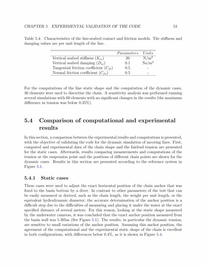
CHAPTER 5. EXPERIMENTAL VALIDATION OF THE CODE 53
Table 5.4: Characteristics of the line-seabed contact and friction models. The stiffness anddamping values are per unit length of the line.
Parameters UnitsVertical seabed stiffness (Ksc) 20 N/m2
Vertical seabed damping (Dsc) 0.1 Ns/m2
Tangential friction coefficient (Cft) 0.5 -Normal friction coefficient (Cfn) 0.5 -
For the computations of the line static shape and the computation of the dynamic cases,30 elements were used to discretize the chain. A sensitivity analysis was performed runningseveral simulations with 60 elements with no significant changes in the results (the maximumdifference in tension was below 0.35%).
5.4 Comparison of computational and experimental
results
In this section, a comparison between the experimental results and computations is presented,with the objective of validating the code for the dynamic simulation of mooring lines. First,computed and experimental data of the chain shape and the fairlead tension are presentedfor the static cases. Afterwards, results comparing measurements and computations of thetension at the suspension point and the positions of different chain points are shown for thedynamic cases. Results in this section are presented according to the reference system inFigure 5.1.
5.4.1 Static cases
These cases were used to adjust the exact horizontal position of the chain anchor that wasfixed to the basin bottom by a diver. In contrast to other parameters of the test that canbe easily measured or derived, such as the chain length, the weight per unit length, or theequivalent hydrodynamic diameter; the accurate determination of the anchor position is adifficult step due to the difficulties of measuring and placing it under the water at the exactspecified distance of several meters. For this reason, looking at the static shape measuredby the underwater cameras, it was concluded that the exact anchor position measured fromthe basin wall was 5.305m (See Figure 5.1). The results, in particular the dynamic tension,are sensitive to small variations of the anchor position. Assuming this anchor position, theagreement of the computational and the experimental static shape of the chain is excellentin both configurations, with differences below 0.4%, as it is shown in Figure 5.4.

CHAPTER 5. EXPERIMENTAL VALIDATION OF THE CODE 54
Figure 5.4: Comparison of the computed and experimental static shapes for bothline configurations
Table 5.5 shows the difference between the computed tension at the fairlead and the exper-imental measurement for both configurations. The error in the predicted static tension isbelow 2%.
Table 5.5: Comparison of static fairlead tension expressed in Newtons.
Configuration 1 Configuration 2Experimental 8.13 14.48Computation 8.10 14.70Difference 0.37% 1.52%
5.4.2 Dynamic cases: tension at the fairlead
Figures 5.5 and 5.6 show the comparison between the numerical predictions and the ex-periments for the different periods of the motion prescribed at the fairlead of the chain forConfiguration 1 and Configuration 2, respectively. The plots show the fairlead tension ofthe chain against the fairlead position. The initial transients have been eliminated and thedata are plotted once the stationary state has been reached. The arrows represent the senseof the dynamic loop: higher tensions are achieved when the fairlead of the chain is moving
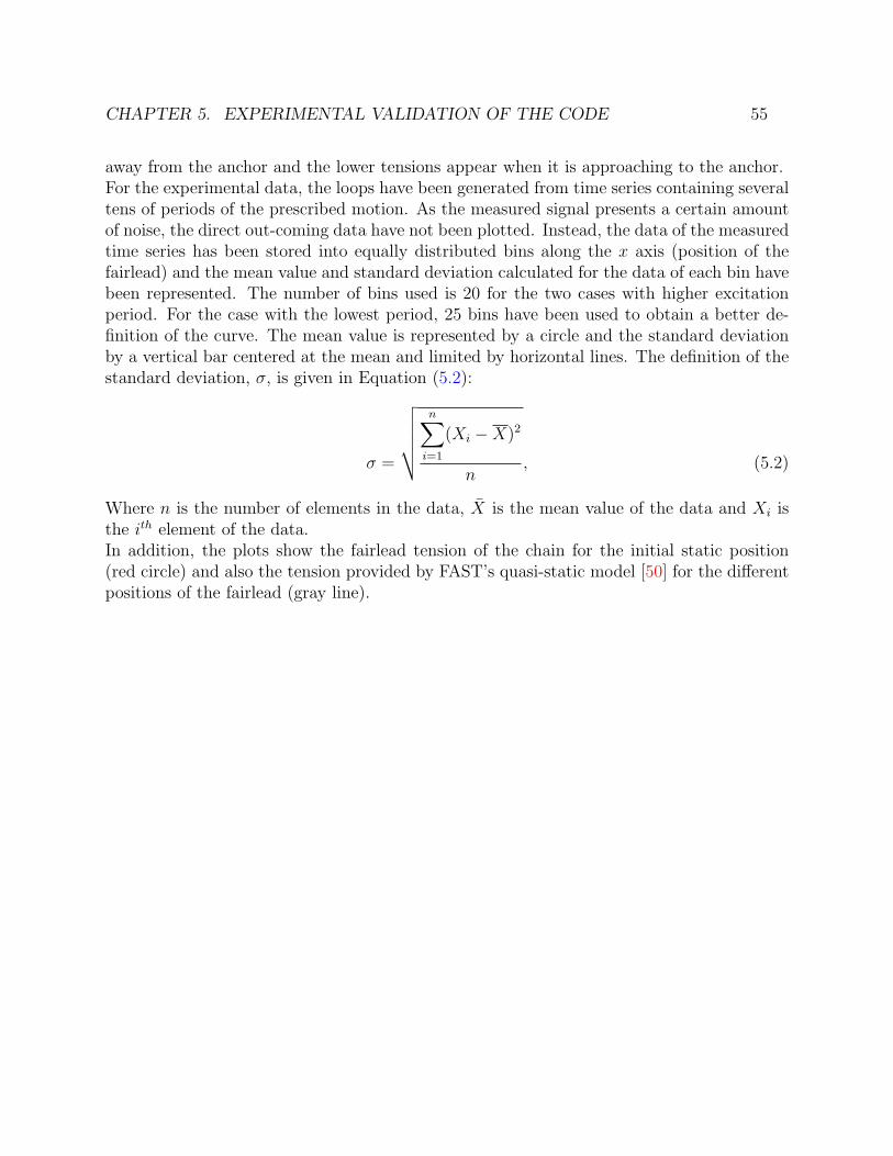
CHAPTER 5. EXPERIMENTAL VALIDATION OF THE CODE 55
away from the anchor and the lower tensions appear when it is approaching to the anchor.For the experimental data, the loops have been generated from time series containing severaltens of periods of the prescribed motion. As the measured signal presents a certain amountof noise, the direct out-coming data have not been plotted. Instead, the data of the measuredtime series has been stored into equally distributed bins along the x axis (position of thefairlead) and the mean value and standard deviation calculated for the data of each bin havebeen represented. The number of bins used is 20 for the two cases with higher excitationperiod. For the case with the lowest period, 25 bins have been used to obtain a better de-finition of the curve. The mean value is represented by a circle and the standard deviationby a vertical bar centered at the mean and limited by horizontal lines. The definition of thestandard deviation, σ, is given in Equation (5.2):
σ =
√√√√√ n∑i=1
(Xi −X)2
n, (5.2)
Where n is the number of elements in the data, X is the mean value of the data and Xi isthe ith element of the data.In addition, the plots show the fairlead tension of the chain for the initial static position(red circle) and also the tension provided by FAST’s quasi-static model [50] for the differentpositions of the fairlead (gray line).
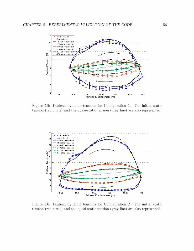
CHAPTER 5. EXPERIMENTAL VALIDATION OF THE CODE 56
Figure 5.5: Fairlead dynamic tensions for Configuration 1. The initial statictension (red circle) and the quasi-static tension (gray line) are also represented.
Figure 5.6: Fairlead dynamic tensions for Configuration 2. The initial statictension (red circle) and the quasi-static tension (gray line) are also represented.
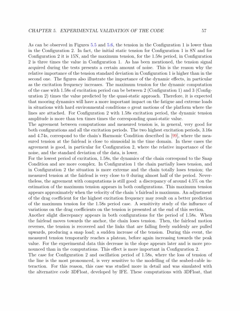
CHAPTER 5. EXPERIMENTAL VALIDATION OF THE CODE 57
As can be observed in Figures 5.5 and 5.6, the tension in the Configuration 1 is lower thanin the Configuration 2. In fact, the initial static tension for Configuration 1 is 8N and forConfiguration 2 it is 15N, and the maximum tension, for the 1.58s period, in Configuration2 is three times the value in Configuration 1. As has been mentioned, the tension signalacquired during the tests presents a certain amount of noise. This is the reason why therelative importance of the tension standard deviation in Configuration 1 is higher than in thesecond one. The figures also illustrate the importance of the dynamic effects, in particularas the excitation frequency increases. The maximum tension for the dynamic computationof the case with 1.58s of excitation period can be between 2 (Configuration 1) and 3 (Config-uration 2) times the value predicted by the quasi-static approach. Therefore, it is expectedthat mooring dynamics will have a more important impact on the fatigue and extreme loadsin situations with hard environmental conditions o great motions of the platform where thelines are attached. For Configuration 2 with 1.58s excitation period, the dynamic tensionamplitude is more than ten times times the corresponding quasi-static value.The agreement between computations and measured tension is, in general, very good forboth configurations and all the excitation periods. The two highest excitation periods, 3.16sand 4.74s, correspond to the chain’s Harmonic Condition described in [99], where the mea-sured tension at the fairlead is close to sinusoidal in the time domain. In these cases theagreement is good, in particular for Configuration 2, where the relative importance of thenoise, and the standard deviation of the data, is lower.For the lowest period of excitation, 1.58s, the dynamics of the chain correspond to the SnapCondition and are more complex. In Configuration 1 the chain partially loses tension, andin Configuration 2 the situation is more extreme and the chain totally loses tension; themeasured tension at the fairlead is very close to 0 during almost half of the period. Never-theless, the agreement with computations is still good: a discrepancy of around 4.5% on theestimation of the maximum tension appears in both configurations. This maximum tensionappears approximately when the velocity of the chain ’s fairlead is maximum. An adjustmentof the drag coefficient for the highest excitation frequency may result on a better predictionof the maximum tension for the 1.58s period case. A sensitivity study of the influence ofvariations on the drag coefficients on the tension is presented at the end of this section.Another slight discrepancy appears in both configurations for the period of 1.58s. Whenthe fairlead moves towards the anchor, the chain loses tension. Then, the fairlead motionreverses, the tension is recovered and the links that are falling freely suddenly are pulledupwards, producing a snap load; a sudden increase of the tension. During this event, themeasured tension temporarily reaches a plateau, before again increasing towards the peakvalue. For the experimental data this decrease in the slope appears later and is more pro-nounced than in the computations. This effect is more important in Configuration 2.The case for Configuration 2 and oscillation period of 1.58s, where the loss of tension ofthe line is the most pronounced, is very sensitive to the modelling of the seabed-cable in-teraction. For this reason, this case was studied more in detail and was simulated withthe alternative code 3DFloat, developed by IFE. These computations with 3DFloat, that
CHAPTER 5. EXPERIMENTAL VALIDATION OF THE CODE 58
are shown in the following discussion, were computed by Tor Anders Nygaard, from IFE.3DFloat [22] is based on a nonlinear co-rotated FEM approach, with three translational andthree rotational DOFs at each node. The cable elements are Euler-Bernoulli beams, wherethe bending stiffness is turned off for chain mooring lines. Both codes, 3DFloat and OPASS,have elements that maintain axial stiffness also when tension is lost, in contrast to the realchain. This fact can affect the behaviour for the part of the chain resting on the seafloor.Both models take the seafloor into account with a seabed contact model. Nodes that dropbelow the defined seafloor, get an applied vertical force that is proportional to the verticaldistance to the seafloor. In addition, linear damping is applied to nodes below the seafloorin the vertical direction. Both codes scale the linear damping with the distance up to theseafloor. 3DFloat also applies a limiter to the damping. In contrast with OPASS, 3DFloatuses no friction for the computations, but applies a horizontal damping to the nodes in con-tact with the seabed, that is not present in OPASS.Figure 5.7 shows the effect of eliminating the seabed-cable friction on the tension computedwith OPASS for the mentioned sensitive case of period 1.58s and Configuration 2. Aftera few periods of excitation, an oscillation is generated in the part of the loop where thesuspension point moves from the minimum position towards the maximum position and thechain is being lifted quickly off the seafloor. This effect does not arise in any of the othercases studied in this work when the seabed friction model is disabled.
Figure 5.7: Effect of seabed friction on the fairlead tension computed withOPASS for 1.58s period and Configuration 2

CHAPTER 5. EXPERIMENTAL VALIDATION OF THE CODE 59
When the considered case is simulated with 3DFloat, a similar effect arise (see Figure 5.8);if no damping is applied to the nodes in contact with the seabed, an oscillation appearswhen the line is recovering the tension. But if enough damping is applied in the vertical andhorizontal direction to the nodes in contact with the seabed, this dynamics disappears.
Figure 5.8: Effect of seabed damping on the fairlead tension computed with3DFloat for 1.58s period and Configuration 2
Apparently, these dynamics are caused by small motions of the nodes of the line resting onthe seabed during the tension-less portion of the dynamic loop. The introduction of seabedfriction in the OPASS model or seabed damping in the 3DFloat model avoid these smallnodal displacements and, consequently, the oscillations are not generated. These dynamicsare not present in the experimental results, due to the friction of the chain with the bottomof the basin. This case highlights the importance of a correct modelling of the line-seabedinteraction to avoid the generation of instabilities in highly dynamic situations with pro-nounced loss of tension in the chain.Figure 5.9 shows how the two models agree well for the 1.58s period case, considering themodelling differences, once the friction is included in OPASS and the seabed damping isincluded in 3DFloat. The results are not sensitive to further increases of friction or dampinglevels beyond damping the oscillations seen in the Figure 5.7 and Figure 5.8. For the largerperiods the results are not sensitive to the seabed model and both tools provide almostidentical tension.
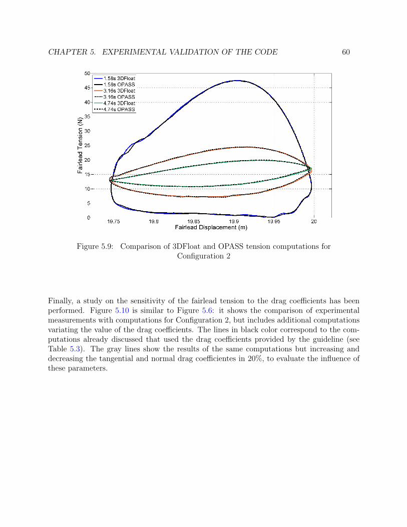
CHAPTER 5. EXPERIMENTAL VALIDATION OF THE CODE 60
Figure 5.9: Comparison of 3DFloat and OPASS tension computations forConfiguration 2
Finally, a study on the sensitivity of the fairlead tension to the drag coefficients has beenperformed. Figure 5.10 is similar to Figure 5.6: it shows the comparison of experimentalmeasurements with computations for Configuration 2, but includes additional computationsvariating the value of the drag coefficients. The lines in black color correspond to the com-putations already discussed that used the drag coefficients provided by the guideline (seeTable 5.3). The gray lines show the results of the same computations but increasing anddecreasing the tangential and normal drag coefficientes in 20%, to evaluate the influence ofthese parameters.
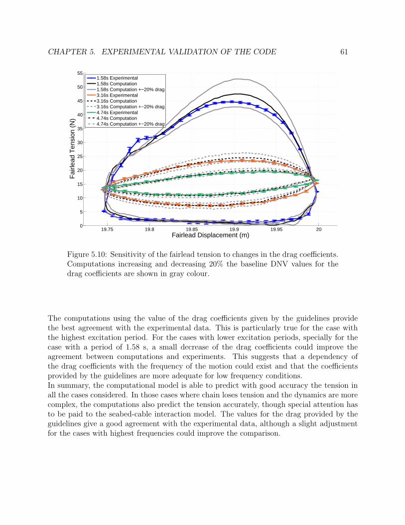
CHAPTER 5. EXPERIMENTAL VALIDATION OF THE CODE 61
19.75 19.8 19.85 19.9 19.95 200
5
10
15
20
25
30
35
40
45
50
55
Fairlead Displacement (m)
Fai
rlead
Ten
sion
(N
)
1.58s Experimental1.58s Computation1.58s Computation +−20% drag3.16s Experimental3.16s Computation3.16s Computation +−20% drag4.74s Experimental4.74s Computation4.74s Computation +−20% drag
Figure 5.10: Sensitivity of the fairlead tension to changes in the drag coefficients.Computations increasing and decreasing 20% the baseline DNV values for thedrag coefficients are shown in gray colour.
The computations using the value of the drag coefficients given by the guidelines providethe best agreement with the experimental data. This is particularly true for the case withthe highest excitation period. For the cases with lower excitation periods, specially for thecase with a period of 1.58 s, a small decrease of the drag coefficients could improve theagreement between computations and experiments. This suggests that a dependency ofthe drag coefficients with the frequency of the motion could exist and that the coefficientsprovided by the guidelines are more adequate for low frequency conditions.In summary, the computational model is able to predict with good accuracy the tension inall the cases considered. In those cases where chain loses tension and the dynamics are morecomplex, the computations also predict the tension accurately, though special attention hasto be paid to the seabed-cable interaction model. The values for the drag provided by theguidelines give a good agreement with the experimental data, although a slight adjustmentfor the cases with highest frequencies could improve the comparison.
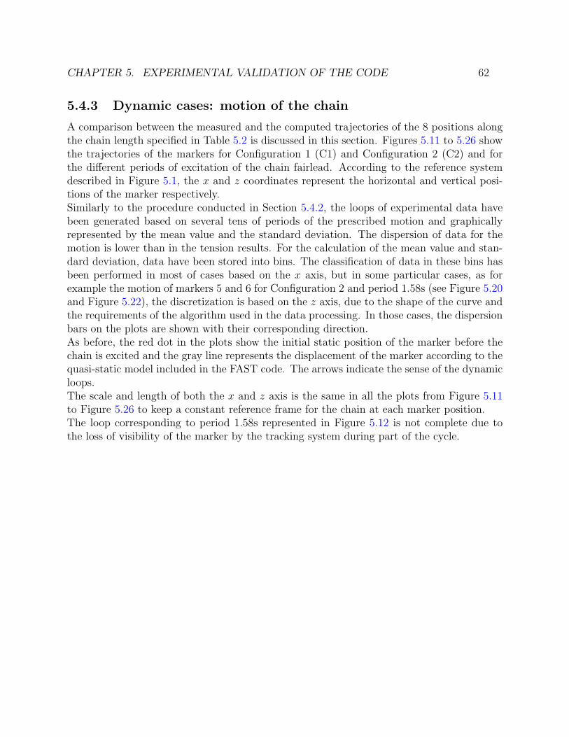
CHAPTER 5. EXPERIMENTAL VALIDATION OF THE CODE 62
5.4.3 Dynamic cases: motion of the chain
A comparison between the measured and the computed trajectories of the 8 positions alongthe chain length specified in Table 5.2 is discussed in this section. Figures 5.11 to 5.26 showthe trajectories of the markers for Configuration 1 (C1) and Configuration 2 (C2) and forthe different periods of excitation of the chain fairlead. According to the reference systemdescribed in Figure 5.1, the x and z coordinates represent the horizontal and vertical posi-tions of the marker respectively.Similarly to the procedure conducted in Section 5.4.2, the loops of experimental data havebeen generated based on several tens of periods of the prescribed motion and graphicallyrepresented by the mean value and the standard deviation. The dispersion of data for themotion is lower than in the tension results. For the calculation of the mean value and stan-dard deviation, data have been stored into bins. The classification of data in these bins hasbeen performed in most of cases based on the x axis, but in some particular cases, as forexample the motion of markers 5 and 6 for Configuration 2 and period 1.58s (see Figure 5.20and Figure 5.22), the discretization is based on the z axis, due to the shape of the curve andthe requirements of the algorithm used in the data processing. In those cases, the dispersionbars on the plots are shown with their corresponding direction.As before, the red dot in the plots show the initial static position of the marker before thechain is excited and the gray line represents the displacement of the marker according to thequasi-static model included in the FAST code. The arrows indicate the sense of the dynamicloops.The scale and length of both the x and z axis is the same in all the plots from Figure 5.11to Figure 5.26 to keep a constant reference frame for the chain at each marker position.The loop corresponding to period 1.58s represented in Figure 5.12 is not complete due tothe loss of visibility of the marker by the tracking system during part of the cycle.
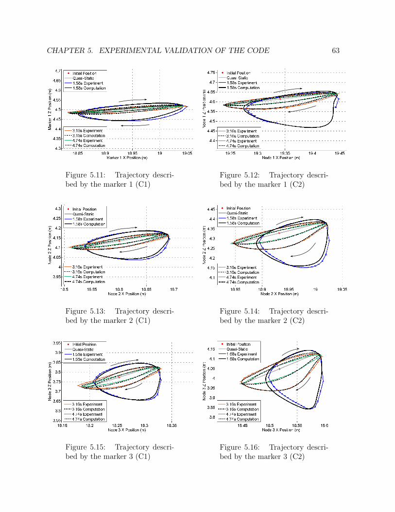
CHAPTER 5. EXPERIMENTAL VALIDATION OF THE CODE 63
Figure 5.11: Trajectory descri-bed by the marker 1 (C1)
Figure 5.12: Trajectory descri-bed by the marker 1 (C2)
Figure 5.13: Trajectory descri-bed by the marker 2 (C1)
Figure 5.14: Trajectory descri-bed by the marker 2 (C2)
Figure 5.15: Trajectory descri-bed by the marker 3 (C1)
Figure 5.16: Trajectory descri-bed by the marker 3 (C2)

CHAPTER 5. EXPERIMENTAL VALIDATION OF THE CODE 64
Figure 5.17: Trajectory descri-bed by the marker 4 (C1)
Figure 5.18: Trajectory descri-bed by the marker 4 (C2)
Figure 5.19: Trajectory descri-bed by the marker 5 (C1)
Figure 5.20: Trajectory descri-bed by the marker 5 (C2)
Figure 5.21: Trajectory descri-bed by the marker 6 (C1)
Figure 5.22: Trajectory descri-bed by the marker 6 (C2)
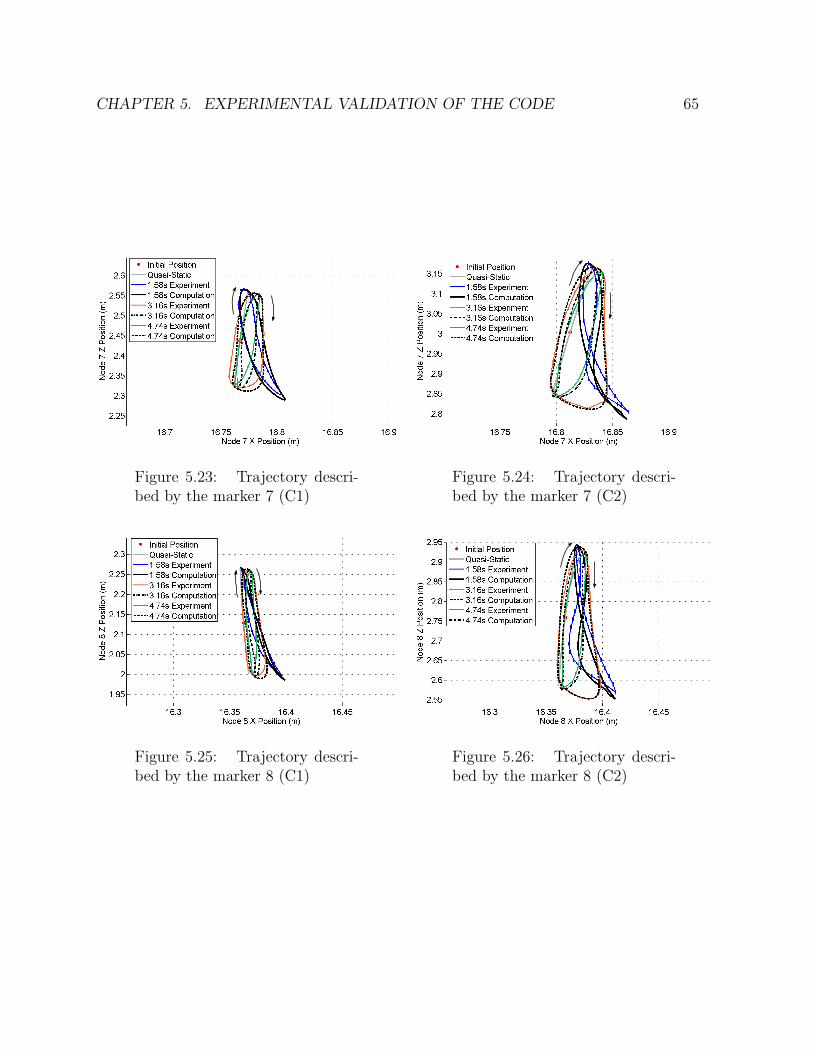
CHAPTER 5. EXPERIMENTAL VALIDATION OF THE CODE 65
Figure 5.23: Trajectory descri-bed by the marker 7 (C1)
Figure 5.24: Trajectory descri-bed by the marker 7 (C2)
Figure 5.25: Trajectory descri-bed by the marker 8 (C1)
Figure 5.26: Trajectory descri-bed by the marker 8 (C2)
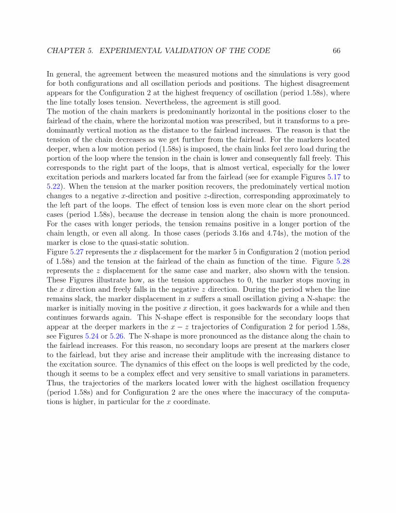
CHAPTER 5. EXPERIMENTAL VALIDATION OF THE CODE 66
In general, the agreement between the measured motions and the simulations is very goodfor both configurations and all oscillation periods and positions. The highest disagreementappears for the Configuration 2 at the highest frequency of oscillation (period 1.58s), wherethe line totally loses tension. Nevertheless, the agreement is still good.The motion of the chain markers is predominantly horizontal in the positions closer to thefairlead of the chain, where the horizontal motion was prescribed, but it transforms to a pre-dominantly vertical motion as the distance to the fairlead increases. The reason is that thetension of the chain decreases as we get further from the fairlead. For the markers locateddeeper, when a low motion period (1.58s) is imposed, the chain links feel zero load during theportion of the loop where the tension in the chain is lower and consequently fall freely. Thiscorresponds to the right part of the loops, that is almost vertical, especially for the lowerexcitation periods and markers located far from the fairlead (see for example Figures 5.17 to5.22). When the tension at the marker position recovers, the predominately vertical motionchanges to a negative x-direction and positive z-direction, corresponding approximately tothe left part of the loops. The effect of tension loss is even more clear on the short periodcases (period 1.58s), because the decrease in tension along the chain is more pronounced.For the cases with longer periods, the tension remains positive in a longer portion of thechain length, or even all along. In those cases (periods 3.16s and 4.74s), the motion of themarker is close to the quasi-static solution.Figure 5.27 represents the x displacement for the marker 5 in Configuration 2 (motion periodof 1.58s) and the tension at the fairlead of the chain as function of the time. Figure 5.28represents the z displacement for the same case and marker, also shown with the tension.These Figures illustrate how, as the tension approaches to 0, the marker stops moving inthe x direction and freely falls in the negative z direction. During the period when the lineremains slack, the marker displacement in x suffers a small oscillation giving a N-shape: themarker is initially moving in the positive x direction, it goes backwards for a while and thencontinues forwards again. This N-shape effect is responsible for the secondary loops thatappear at the deeper markers in the x − z trajectories of Configuration 2 for period 1.58s,see Figures 5.24 or 5.26. The N-shape is more pronounced as the distance along the chain tothe fairlead increases. For this reason, no secondary loops are present at the markers closerto the fairlead, but they arise and increase their amplitude with the increasing distance tothe excitation source. The dynamics of this effect on the loops is well predicted by the code,though it seems to be a complex effect and very sensitive to small variations in parameters.Thus, the trajectories of the markers located lower with the highest oscillation frequency(period 1.58s) and for Configuration 2 are the ones where the inaccuracy of the computa-tions is higher, in particular for the x coordinate.

CHAPTER 5. EXPERIMENTAL VALIDATION OF THE CODE 67
Figure 5.27: X position and tension for marker 5 (Conf. 2, period 1.58s)
Figure 5.28: Z position and tension for marker 5 (Conf. 2, period 1.58s)
CHAPTER 5. EXPERIMENTAL VALIDATION OF THE CODE 68
5.5 Concluding remarks
The dynamic mooring line code developed in this research has been successfully validatedagainst experimental data for static and dynamic conditions. Two configurations of thechain have been studied, with different tension levels. The agreement between computationsand experimental results is very good for the chain fairlead tension and also for the motionof the chain at the diverse positions considered.In the static cases, both the shape of the line and the tension at the suspension point comparevery well between the computations and the experiments.For the dynamic validation, the chain has been excited with a prescribed motion at thefairlead with three oscillation periods, producing different dynamic conditions, includingharmonic response, loss of tension and snap loading. The code is able to predict the motionof the chain and the tension with precision in all these conditions.The added mass and drag coefficients for the chain, that have been chosen from guidelines,in general, represent with accuracy the hydrodynamic loads.The importance of including dynamic effects on the prediction of the mooring line loads hasbeen shown; the maximum tension can be between 2 and 3 times the value computed bythe quasi-static approach when high excitation frequency is imposed. The tension amplitudecan be more than ten times times the corresponding quasi-static value.For the cases with the lowest excitation period, where the line slacks, the computed andmeasured tension agree well, although a slight difference appears during the snap loads oncetension recovers. In these cases, the maximum tension is overpredicted by the code by around4.5%. These differences could be due to the fact that the drag coefficients could present adependency with the motion frequency and the values from guidelines could be tuned for thecases with the low excitation frequencies. Regarding the chain motions, those cases wherethe chain loses tension present the highest inaccuracies in the numerical results, especiallyin the lowest part of the chain, though the results are still good.In the cases with higher tension level and higher excitation frequency, the simulation resultsare particularly sensitive to the cable-seabed interaction model. This was confirmed also byverification against the 3DFloat code of IFE. The computational model is able to predictthe tension with accuracy, but the modelling of the seabed friction should not be neglected.
69
Chapter 6
Mooring dynamics on fatigue andultimate loads
6.1 Abstract
In this chapter, the OPASS code, developed and experimentally validated in previous chap-ters, is used for an extensive assessment of the effect of mooring dynamics on the fatigueand ultimate loads of different floating wind turbines. The loads were computed followingthe floating wind turbines IEC 61400-3 Edition 1 guideline [47].Three platforms topologies (semisubmersible, spar-buoy and TLP), representing the threemain methods to achieve the stability, are assumed to be installed at the same 200 m depthlocation in the Irish coast supporting the same 5 MW wind turbine.For each platform, the fatigue and ultimate loads are computed with the FAST integratedfloating wind turbine simulation code using both, a quasi-static and the OPASS fully dynamicmoorings model. More than 20,000 load cases are launched and postprocessed following theIEC 61400-3 guideline. The methodology and results presented in this chapter, have beenpublished in [13] and [8].As Chapter 3 discussed, several authors have compared coupled simulations using a quasi-static and a dynamic model for different floating platforms, having most of these studiesimportant limitations. The following aspects of the research described in this chapter haveto be highlighted, because they contribute to overcome the weaknesses of the previous stu-dies:
1. Fatigue equivalent loads are computed based on all the load case groups requested bythe guideline, not only in individual cases, and are weighted based on their importanceon the turbine lifetime.
2. Extreme loads are also calculated based on all the load case groups requested by theguideline (with the exception of the group 8 that is usually considered benign) and notonly in a limited number of cases.
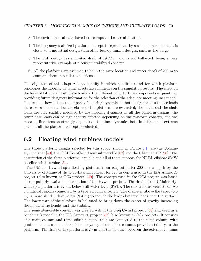
CHAPTER 6. MOORING DYNAMICS ON FATIGUE AND ULTIMATE LOADS 70
3. The environmental data have been computed for a real location.
4. The buoyancy stabilized platform concept is represented by a semisubmersible, that iscloser to a industrial design than other less optimized designs, such as the barge.
5. The TLP design has a limited draft of 19.72 m and is not ballasted, being a veryrepresentative example of a tension stabilized concept.
6. All the platforms are assumed to be in the same location and water depth of 200 m tocompare them in similar conditions.
The objective of this chapter is to identify in which conditions and for which platformtopologies the mooring dynamic effects have influence on the simulation results. The effect onthe level of fatigue and ultimate loads of the different wind turbine components is quantifiedproviding future designers information for the selection of the adequate mooring lines model.The results showed that the impact of mooring dynamics in both fatigue and ultimate loadsincreases as elements located closer to the platform are evaluated; the blade and the shaftloads are only slightly modified by the mooring dynamics in all the platform designs, thetower base loads can be significantly affected depending on the platform concept, and themooring lines tension strongly depends on the lines dynamics both in fatigue and extremeloads in all the platform concepts evaluated.
6.2 Floating wind turbines models
The three platform designs selected for this study, shown in Figure 6.1, are the UMaineHywind spar [49], the OC4 DeepCwind semisubmersible [87] and the UMaine TLP [98]. Thedescription of the three platforms is public and all of them support the NREL offshore 5MWbaseline wind turbine [51].The UMaine Hywind spar floating platform is an adaptation for 200 m sea depth by the
University of Maine of the OC3-Hywind concept for 320 m depth used in the IEA Annex 23project (also known as OC3 project) [49]. The concept used in the OC3 project was basedon the publicly available information of the Hywind project. The draft of the UMaine Hy-wind spar platform is 120 m below still water level (SWL). The substructure consists of twocylindrical regions connected by a tapered conical region. The diameter above the taper (6.5m) is more slender than below (9.4 m) to reduce the hydrodynamic loads near the surface.The lower part of the platform is ballasted to bring down the center of gravity increasingthe metacentric height and the stability.The semisubmersible concept was created within the DeepCwind project [38] and used as abenchmark model in the IEA Annex 30 project [87] (also known as OC4 project). It consistsof a main column and three offset columns that are connected to the main column withpontoons and cross members. The buoyancy of the offset columns provides stability to theplatform. The draft of the platform is 20 m and the distance between the external columns
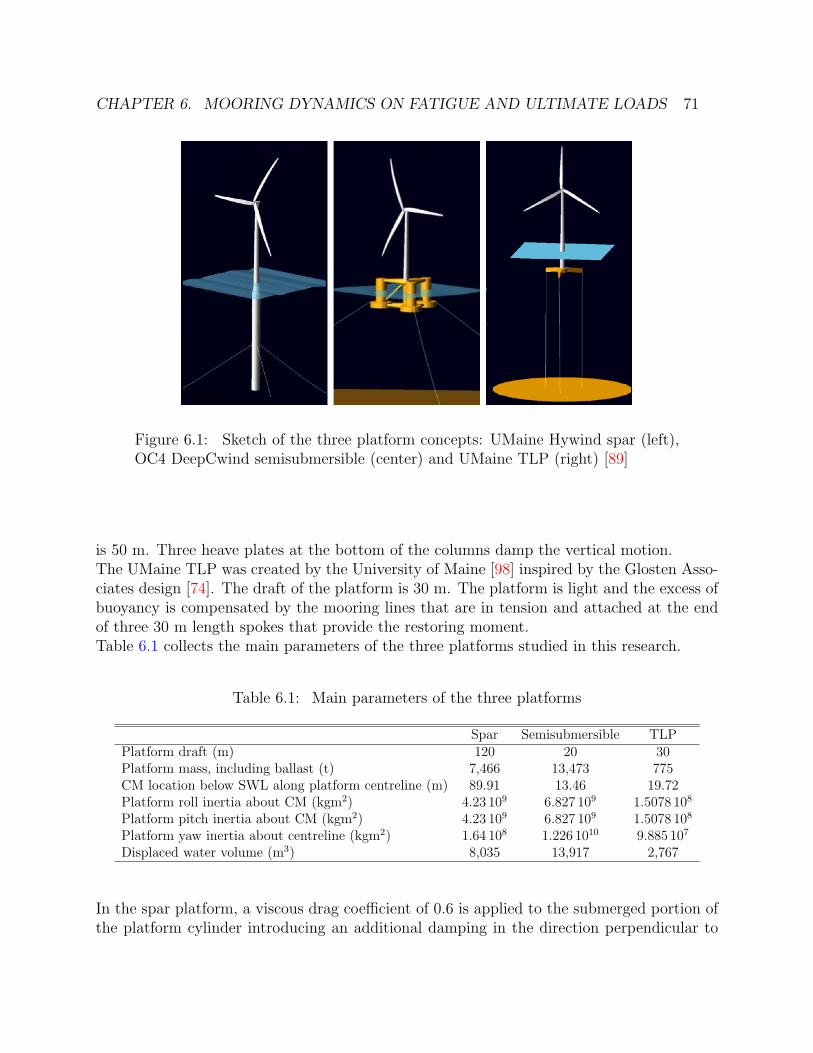
CHAPTER 6. MOORING DYNAMICS ON FATIGUE AND ULTIMATE LOADS 71
Figure 6.1: Sketch of the three platform concepts: UMaine Hywind spar (left),OC4 DeepCwind semisubmersible (center) and UMaine TLP (right) [89]
is 50 m. Three heave plates at the bottom of the columns damp the vertical motion.The UMaine TLP was created by the University of Maine [98] inspired by the Glosten Asso-ciates design [74]. The draft of the platform is 30 m. The platform is light and the excess ofbuoyancy is compensated by the mooring lines that are in tension and attached at the endof three 30 m length spokes that provide the restoring moment.Table 6.1 collects the main parameters of the three platforms studied in this research.
Table 6.1: Main parameters of the three platforms
Spar Semisubmersible TLPPlatform draft (m) 120 20 30Platform mass, including ballast (t) 7,466 13,473 775CM location below SWL along platform centreline (m) 89.91 13.46 19.72Platform roll inertia about CM (kgm2) 4.23 109 6.827 109 1.5078 108
Platform pitch inertia about CM (kgm2) 4.23 109 6.827 109 1.5078 108
Platform yaw inertia about centreline (kgm2) 1.64 108 1.226 1010 9.885 107
Displaced water volume (m3) 8,035 13,917 2,767
In the spar platform, a viscous drag coefficient of 0.6 is applied to the submerged portion ofthe platform cylinder introducing an additional damping in the direction perpendicular to
CHAPTER 6. MOORING DYNAMICS ON FATIGUE AND ULTIMATE LOADS 72
the cylinder axis. Following the model description in [49], additional linear damping coeffi-cient in the surge, sway, heave and yaw degrees of freedom was applied to capture accuratelythe platform dynamics. This additional damping is provided in Table 6.2.
Table 6.2: Additional linear damping for the spar platform
Surge 100 kNs/mSway 100 kNs/mHeave 130 kNs/mYaw 13,000 kNms/rad
For the semisubmersible platform, a viscous drag coefficient was also applied in the cylin-drical elements. The value of the coefficient depends on the element diameter and is shownin Table 6.3. For the heave plates a coefficient of 4.8 was defined, using the diameter of theplates as reference length.
Table 6.3: Viscous drag damping coefficients in the semisubmersible platform elements
Main column 0.56Upper columns 0.61Base columns 0.68Pontoons and cross members 0.63Heave plates 4.80
For the TLP, a viscous drag coefficient of 0.6 was defined for the three spokes and for thesubmerged portion of tower. In addition, the surface at the platform keel was considered asa heave plate with a drag coefficient of 4.8 and a effective radius of 7.5 m.The mooring system of the three platforms is composed of three lines. The spar design hasone downwind line aligned with the nominal wind direction (line 1) and two upwind linesforming 60◦ with the wind direction (lines 2 and 3). For the semisubmersible and the TLP,the configuration is the opposite: one line is upwind and parallel to the nominal wind direc-tion (line 2) and the other two are downwind forming 60◦ with the wind direction (lines 1and 3).The characteristics of the mooring systems are summarized in Table 6.4. A line-seabed con-tact model with no friction was included.

CHAPTER 6. MOORING DYNAMICS ON FATIGUE AND ULTIMATE LOADS 73
Table 6.4: Main parameters of the three mooring systems
Spar Semisubmersible TLPNumber of mooring lines 3 3 3Angle between adjacent lines 120◦ 120◦ 120◦
Depth to anchors below SWL (m) 200 200 200Depth to fairleads below SWL (m) 70.0 14.0 28.5Radius to anchors from platform centreline (m) 445 837.6 30.0Radius to fairleads from platform centreline (m) 5.2 40.868 30.0Unstretched length (m) 468 835.5 171.399Line diameter (m) 0.09 0.0766 0.2216Equivalent mass density (kg/m) 145 113.35 302.89Equivalent extensional stiffness (kN) 384,243 753,600 7,720,000
Parameters in Table 6.4 are sufficient for the construction of a quasi-static mooring model,while for the dynamic model the additional parameters presented in Table 6.5 are required.According to [18] the added mass coefficient was set to 1. A normal drag coefficient of 1.6and no tangential drag were set for all lines based on [25]. A seabed vertical stiffness anddamping were defined for the dynamic line-seabed contact model. The number of elementsof each line were selected after performing a sensitivity study running several simulationswith double number of elements with no significant changes.
Table 6.5: Additional parameters of the three mooring systems used in the dynamic model
Spar Semisubmersible TLPAdded mass coefficient 1.0 1.0 1.0Normal drag coefficient 1.6 1.6 1.6Tangential drag coefficient 0.0 0.0 0.0Structural damping (%) 1.0 1.0 1.0Seabed vertical stiffness (N/m2) 500,000 500,000 500,000Seabed vertical damping (Ns/m2) 30,000 30,000 30,000Number of elements of the line 45 80 40
Finally, for the spar design the lines are attached to the platform using a delta connectionto increase the mooring system stiffness in yaw. Instead of modelling the delta connection,the platform yaw stiffness of the platform was increased with 98340 kNm/rad, as indicatedin [49].The wind turbine supported by the three platforms is the NREL offshore 5 MW baseline,
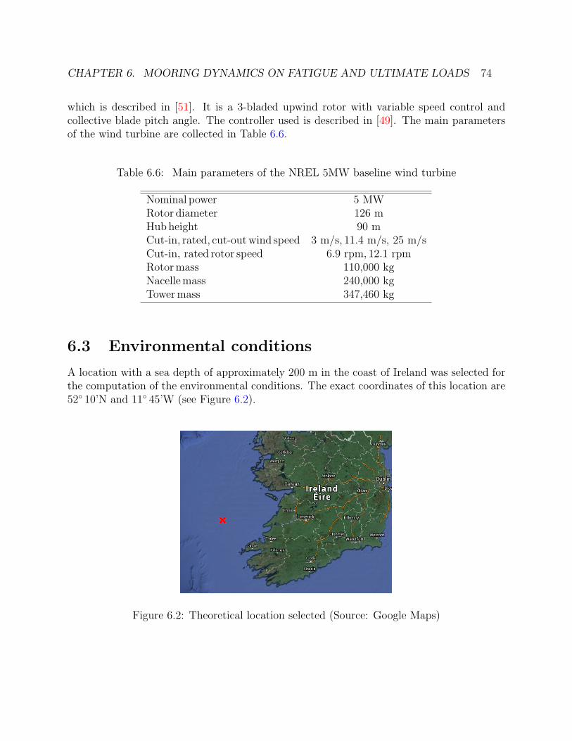
CHAPTER 6. MOORING DYNAMICS ON FATIGUE AND ULTIMATE LOADS 74
which is described in [51]. It is a 3-bladed upwind rotor with variable speed control andcollective blade pitch angle. The controller used is described in [49]. The main parametersof the wind turbine are collected in Table 6.6.
Table 6.6: Main parameters of the NREL 5MW baseline wind turbine
Nominal power 5 MWRotor diameter 126 mHubheight 90 mCut-in, rated, cut-outwind speed 3 m/s, 11.4 m/s, 25 m/sCut-in, rated rotor speed 6.9 rpm, 12.1 rpmRotormass 110,000 kgNacellemass 240,000 kgTowermass 347,460 kg
6.3 Environmental conditions
A location with a sea depth of approximately 200 m in the coast of Ireland was selected forthe computation of the environmental conditions. The exact coordinates of this location are52◦ 10’N and 11◦ 45’W (see Figure 6.2).
Figure 6.2: Theoretical location selected (Source: Google Maps)

CHAPTER 6. MOORING DYNAMICS ON FATIGUE AND ULTIMATE LOADS 75
An hourly wind and wave database between 2004 to 2011 was generated using the Skiron[54] and the WAM [43] models for the wind and the wave respectively. These data were usedto generate the scatter tables that determine the significant wave height (Hs) and referencepeak spectral period (Tp) as function of the wind speed (Vw) required for the definition ofeach particular simulation load case according to the guideline. A Pierson-Moskowitz spec-trum was assumed to represent the wave energy distribution. As the metoceanic model useddid not include surface current data, a 1-year surface current velocity of 0.609 m/s and a50-year surface current velocity of 1.31 m/s were assumed. A summary of the environmentalparameters is provided in Table 6.7.
Table 6.7: Summary of the location metoceanic data
Sea depth 200 mMean significant wave height 2.98 mMean peak spectral period 9.58 s1-year significant wave height 9.82 m1-year peak spectral period 14.30 s50-year significant wave height 11.50 m50-year peak spectral period 15.48 sMean wind speed 10.6 m/sHub height 50-year extreme wind speed (10 minutes mean) 42.5 m/sCharacteristic turbulence intensity at 15 m/s 0.16
6.4 Design load cases simulated for the fatigue and
ultimate loads
The computation of the fatigue and the ultimate loads followed the requirements of the IEC61400-3 guideline [47]. This guideline defines design load cases (DLC) covering all the sig-nificant conditions that an offshore wind turbine may experience. The guideline combinesthe wind turbine operational modes or design situations with external conditions includingthe control actions and the protection system. The load cases are divided into fatigue andultimate cases. The corresponding safety factor was applied to the ultimate loads accordingto the guideline specifications. For the fatigue cases, it has been assumed that wind andwaves are always co-directional to facilitate the postprocessing. This is a simplification ofthe typical definition of the cases, that requires waves and wind with different directions,but does not affect to the conclusions on the effect of mooring dynamics. Yaw errors areincluded in the required load cases. No changes in the sea water level due to tides have beentaken into consideration.
CHAPTER 6. MOORING DYNAMICS ON FATIGUE AND ULTIMATE LOADS 76
The fatigue cases recreate different scenarios, such as power production, power productionfollowed by grid loss, normal shut down and parked. Table 6.8 shows a description of thefatigue load cases. Cases of start-up, parked and fault and installation are usually consideredwith low impact on fatigue loads and were not included in the equivalent loads computation.
Table 6.8: Fatigue load cases definition
Design situation DLCWind
ConditionWaves
Wind-Wavesdirectionality
Seacurrents
Other
Power production 1.2 NTM NSS COD No
Power production+ fault
2.4 NTM NSS COD, UNI NoControl, protection orelectrical faults
Normal shut down 4.1 NWP NSS COD, UNI No
Parked (standingstill/idling)
6.4 NTM NSS COD No
COD: Co-Directional NSS: Normal Sea State NTM: Normal Turbulence Model NWP: Normal Wind Profile
UNI: Uni-Directional
The Rainflow cycle counting method was applied to the fatigue load cases time series toobtain the number and range of cycles. For the calculation of the fatigue equivalent loads,the cycles of each load case are weighted according to the relative importance of the case inthe turbine lifetime. The fatigue equivalent loads were calculated based on 107 cycles in 20years of lifetime with the expression:
Fequivalent =
(∑i niS
mi
Thf
) 1m
(6.1)
where ni is the number of cycles in the load range Si, Th is the duration of the original timehistory, f is the frequency of the equivalent load and m is the inverse S-N material slope.The ultimate load cases recreate extreme scenarios as emergency shutdowns, parked andfault conditions and extreme environmental conditions. Table 6.9 gives a description of theultimate load cases. Details can be found in the guideline [47]. All the load cases requested bythe guideline were computed, with the exception of the case group 8 and a certain number ofsubcases of the 2.2 group. The case group 8 simulates transport, assembly, maintenance andrepair and are usually considered benign. The discarded subcases of the 2.2 group simulate afault in the nacelle yaw angle control, provoking a yaw rotation of the nacelle (yaw runaway)
CHAPTER 6. MOORING DYNAMICS ON FATIGUE AND ULTIMATE LOADS 77
of 360◦. When the yaw angle of the nacelle reaches 180◦, the wind attacks the rotor from adirection opposite to the design condition, and the wind turbine behaviour is very sensitiveto the control design. The controller used is a baseline controller that does not take intoaccount such specific conditions, consequently not being representative of the real conditions.
Table 6.9: Ultimate load cases definition
Design situation DLCWind
ConditionWaves
Wind-Wavesdirectionality
Sea currents Water level Other
Powerproduction
1.1 NTM NSS COD, UNI NCM MSL
1.3 ETM NSS COD, UNI NCM MSL
1.4 ECDNSS orNWH
MIS, wind directionchange
NCM MSL
1.5 EWS NSS COD, UNI NCM MSL
1.6 NTM SSS COD, UNI NCM NWLR
Powerproduction+ fault
2.1 NTM NSS COD, UNI NCM MSL Control fault or loss of network
2.2 NTM NSS COD, UNI NCM MSLProtection system or internal elec-trical fault
2.3 EOGNSS orNWH
COD, UNI NCM MSL Electrical fault, loss of network
Normal shut down 4.2 EOGNSS orNWH
COD, UNI NCM MSL
Emergency shut down 5.1 NTMNSS orNWH
COD, UNI NCM MSL
Parked(standingstill/idling)
6.1EWM
(Turbulent)ESS MIS, MUL ECM EWLR
6.2EWM
(Turbulent)ESS MIS, MUL ECM EWLR Loss of network
6.3EWM
(Turbulent)ESS MIS, MUL ECM EWLR Extreme yaw misalignement
Parked + fault 7.1EWM
(Turbulent)ESS MIS, MUL ECM EWLR
COD: Co-Directional ECD: Extreme Coherent gust with Direction change ECM: Extreme Current Model EOG: Extreme Operating Gust ESS: Extreme Sea State ETM: Extreme Turbulent Model
EWLR: Extreme Water Level Range EWM: Extreme Wind Model EWS: Extreme Wind Shear MIS: Misaligned MSL: Mean Sea Level MUL: Multi-Directional NCM: Normal Current Model
NSS: Normal Sea State NTM: Normal Turbulence Model NWH: Normal Wave Height NWLR: Normal Water Level Range RWM: Reduced Wind speed Model SSS: Severe Sea State
More than 3.500 load cases were simulated for each platform and for each mooring mode-lling approach (around 400 fatigue cases and 3.100 extreme cases). In total more than 20,000cases were computed. The cases were launched in a cluster with 450 cores, taking around 5days the simulation of the whole set. The FAST and OPASS output files were converted toBLADED binary format and BLADED postprocessing tools were used for the computationof the fatigue and ultimate loads.Figure 6.3 shows the reference system for the loads at the different wind turbine components:
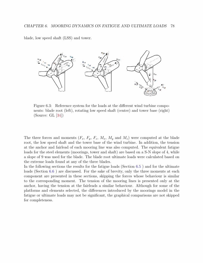
CHAPTER 6. MOORING DYNAMICS ON FATIGUE AND ULTIMATE LOADS 78
blade, low speed shaft (LSS) and tower.
Figure 6.3: Reference system for the loads at the different wind turbine compo-nents: blade root (left), rotating low speed shaft (center) and tower base (right)(Source: GL [34])
The three forces and moments (Fx, Fy, Fz, Mx, My and Mz) were computed at the bladeroot, the low speed shaft and the tower base of the wind turbine. In addition, the tensionat the anchor and fairlead of each mooring line was also computed. The equivalent fatigueloads for the steel elements (moorings, tower and shaft) are based on a S-N slope of 4, whilea slope of 9 was used for the blade. The blade root ultimate loads were calculated based onthe extreme loads found at any of the three blades.In the following sections the results for the fatigue loads (Section 6.5 ) and for the ultimateloads (Section 6.6 ) are discussed. For the sake of brevity, only the three moments at eachcomponent are presented in these sections, skipping the forces whose behaviour is similarto the corresponding moment. The tension of the mooring lines is presented only at theanchor, having the tension at the fairleads a similar behaviour. Although for some of theplatforms and elements selected, the differences introduced by the moorings model in thefatigue or ultimate loads may not be significant, the graphical comparisons are not skippedfor completeness.

CHAPTER 6. MOORING DYNAMICS ON FATIGUE AND ULTIMATE LOADS 79
6.5 Impact of mooring lines dynamics on fatigue loads
6.5.1 Spar fatigue loads
The pitch and roll motions have a great impact on the level of loads of the wind turbinecomponents. The simulations using the quasi-static and the dynamic moorings models pro-vide very similar pitch and roll motions for the spar concept because the fairleads are locatedvery close to the center of rotation of the system. The fatigue analysis reveals no significantdifferences (below 1%) in the equivalent loads obtained with the two mooring models for thewind turbine components (blades, shaft and tower), see Figures 6.4, 6.5 and 6.6.On the other hand, the additional drag introduced by the dynamic model of the lines slightlyreduces the translational surge and sway motions of the platform in comparison with thequasi-static model. Although this implies opposite effects on the tension of the lines (thedrag would increase the line tension for a prescribed movement, but the additional dampingreduces the motions of the line fairlead decreasing the peaks of tension), the combined effectresults in a reduction on the tension peaks. Figure 6.7 shows significant differences for thefatigue equivalent tension of the moorings computed with the quasi-static and the dynamicmodels. The quasi-static model provides up to 8% higher tensions than the dynamic.As the environmental conditions of the fatigue cases are moderate, the accelerations of theplatform are not high and the inertial effect of the lines does not have an important impacton the computation of the spar fatigue loads.
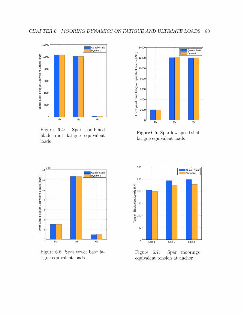
CHAPTER 6. MOORING DYNAMICS ON FATIGUE AND ULTIMATE LOADS 80
Mx My Mz0
2000
4000
6000
8000
10000
12000
Bla
de R
oot F
atig
ue E
quiv
alen
t Loa
ds (
kNm
)
Quasi−StaticDynamic
Figure 6.4: Spar combinedblade root fatigue equivalentloads
Mx My Mz0
2000
4000
6000
8000
10000
12000
14000
Low
Spe
ed S
haft
Fat
igue
Equ
ival
ent L
oads
(kN
m)
Quasi−StaticDynamic
Figure 6.5: Spar low speed shaftfatigue equivalent loads
Mx My Mz0
2
4
6
8
10
12
14x 10
4
Tow
er B
ase
Fat
igue
Equ
ival
ent L
oads
(kN
m)
Quasi−StaticDynamic
Figure 6.6: Spar tower base fa-tigue equivalent loads
Line 1 Line 2 Line 30
50
100
150
200
250
300
Ten
sion
Equ
ival
ent L
oads
(kN
)
Quasi−StaticDynamic
Figure 6.7: Spar mooringsequivalent tension at anchor
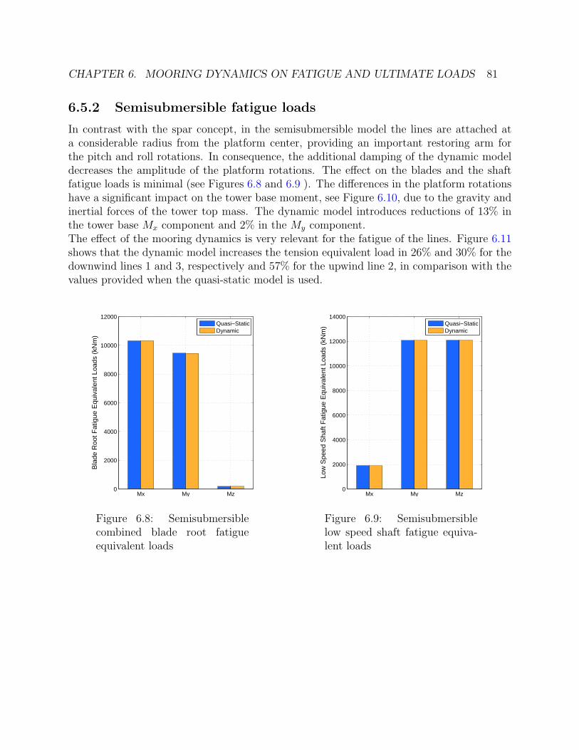
CHAPTER 6. MOORING DYNAMICS ON FATIGUE AND ULTIMATE LOADS 81
6.5.2 Semisubmersible fatigue loads
In contrast with the spar concept, in the semisubmersible model the lines are attached ata considerable radius from the platform center, providing an important restoring arm forthe pitch and roll rotations. In consequence, the additional damping of the dynamic modeldecreases the amplitude of the platform rotations. The effect on the blades and the shaftfatigue loads is minimal (see Figures 6.8 and 6.9 ). The differences in the platform rotationshave a significant impact on the tower base moment, see Figure 6.10, due to the gravity andinertial forces of the tower top mass. The dynamic model introduces reductions of 13% inthe tower base Mx component and 2% in the My component.The effect of the mooring dynamics is very relevant for the fatigue of the lines. Figure 6.11shows that the dynamic model increases the tension equivalent load in 26% and 30% for thedownwind lines 1 and 3, respectively and 57% for the upwind line 2, in comparison with thevalues provided when the quasi-static model is used.
Mx My Mz0
2000
4000
6000
8000
10000
12000
Bla
de R
oot F
atig
ue E
quiv
alen
t Loa
ds (
kNm
)
Quasi−StaticDynamic
Figure 6.8: Semisubmersiblecombined blade root fatigueequivalent loads
Mx My Mz0
2000
4000
6000
8000
10000
12000
14000Lo
w S
peed
Sha
ft F
atig
ue E
quiv
alen
t Loa
ds (
kNm
)
Quasi−StaticDynamic
Figure 6.9: Semisubmersiblelow speed shaft fatigue equiva-lent loads
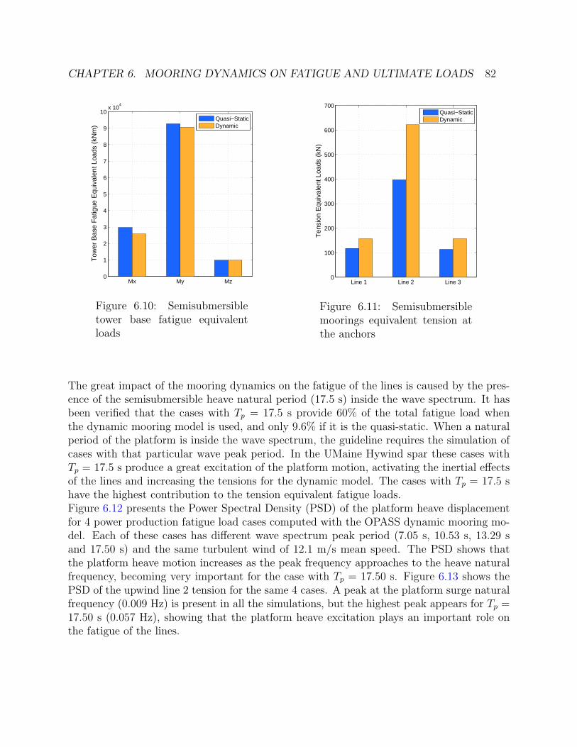
CHAPTER 6. MOORING DYNAMICS ON FATIGUE AND ULTIMATE LOADS 82
Mx My Mz0
1
2
3
4
5
6
7
8
9
10x 10
4
Tow
er B
ase
Fat
igue
Equ
ival
ent L
oads
(kN
m)
Quasi−StaticDynamic
Figure 6.10: Semisubmersibletower base fatigue equivalentloads
Line 1 Line 2 Line 30
100
200
300
400
500
600
700
Ten
sion
Equ
ival
ent L
oads
(kN
)
Quasi−StaticDynamic
Figure 6.11: Semisubmersiblemoorings equivalent tension atthe anchors
The great impact of the mooring dynamics on the fatigue of the lines is caused by the pres-ence of the semisubmersible heave natural period (17.5 s) inside the wave spectrum. It hasbeen verified that the cases with Tp = 17.5 s provide 60% of the total fatigue load whenthe dynamic mooring model is used, and only 9.6% if it is the quasi-static. When a naturalperiod of the platform is inside the wave spectrum, the guideline requires the simulation ofcases with that particular wave peak period. In the UMaine Hywind spar these cases withTp = 17.5 s produce a great excitation of the platform motion, activating the inertial effectsof the lines and increasing the tensions for the dynamic model. The cases with Tp = 17.5 shave the highest contribution to the tension equivalent fatigue loads.Figure 6.12 presents the Power Spectral Density (PSD) of the platform heave displacementfor 4 power production fatigue load cases computed with the OPASS dynamic mooring mo-del. Each of these cases has different wave spectrum peak period (7.05 s, 10.53 s, 13.29 sand 17.50 s) and the same turbulent wind of 12.1 m/s mean speed. The PSD shows thatthe platform heave motion increases as the peak frequency approaches to the heave naturalfrequency, becoming very important for the case with Tp = 17.50 s. Figure 6.13 shows thePSD of the upwind line 2 tension for the same 4 cases. A peak at the platform surge naturalfrequency (0.009 Hz) is present in all the simulations, but the highest peak appears for Tp =17.50 s (0.057 Hz), showing that the platform heave excitation plays an important role onthe fatigue of the lines.
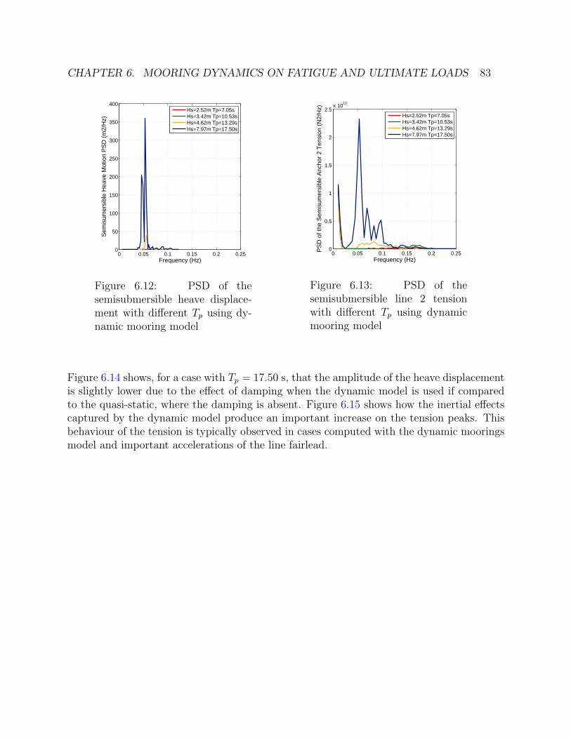
CHAPTER 6. MOORING DYNAMICS ON FATIGUE AND ULTIMATE LOADS 83
0 0.05 0.1 0.15 0.2 0.250
50
100
150
200
250
300
350
400S
emis
umer
sibl
e H
eave
Mot
ion
PS
D (
m2/
Hz)
Frequency (Hz)
Hs=2.52m Tp=7.05sHs=3.42m Tp=10.53sHs=4.62m Tp=13.29sHs=7.97m Tp=17.50s
Figure 6.12: PSD of thesemisubmersible heave displace-ment with different Tp using dy-namic mooring model
0 0.05 0.1 0.15 0.2 0.250
0.5
1
1.5
2
2.5x 10
12
PS
D o
f the
Sem
isum
ersi
ble
Anc
hor
2 T
ensi
on (
N2/
Hz)
Frequency (Hz)
Hs=2.52m Tp=7.05sHs=3.42m Tp=10.53sHs=4.62m Tp=13.29sHs=7.97m Tp=17.50s
Figure 6.13: PSD of thesemisubmersible line 2 tensionwith different Tp using dynamicmooring model
Figure 6.14 shows, for a case with Tp = 17.50 s, that the amplitude of the heave displacementis slightly lower due to the effect of damping when the dynamic model is used if comparedto the quasi-static, where the damping is absent. Figure 6.15 shows how the inertial effectscaptured by the dynamic model produce an important increase on the tension peaks. Thisbehaviour of the tension is typically observed in cases computed with the dynamic mooringsmodel and important accelerations of the line fairlead.
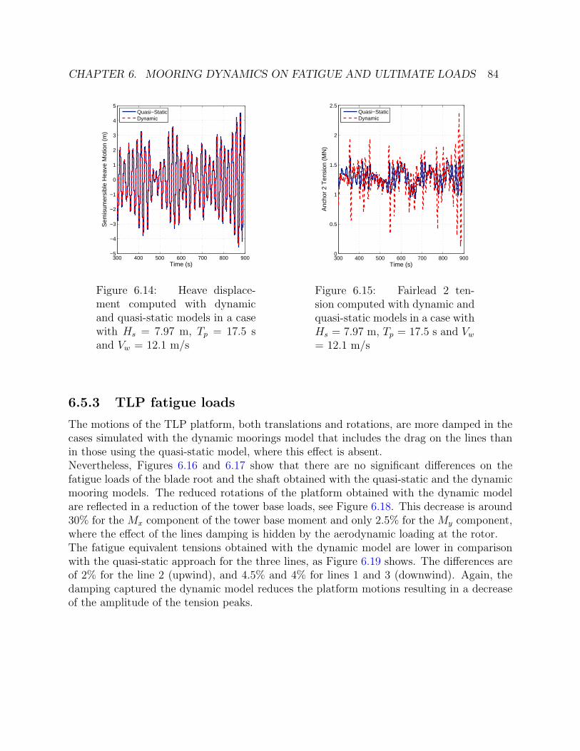
CHAPTER 6. MOORING DYNAMICS ON FATIGUE AND ULTIMATE LOADS 84
300 400 500 600 700 800 900−5
−4
−3
−2
−1
0
1
2
3
4
5S
emis
umer
sibl
e H
eave
Mot
ion
(m)
Time (s)
Quasi−StaticDynamic
Figure 6.14: Heave displace-ment computed with dynamicand quasi-static models in a casewith Hs = 7.97 m, Tp = 17.5 sand Vw = 12.1 m/s
300 400 500 600 700 800 9000
0.5
1
1.5
2
2.5
Anc
hor
2 T
ensi
on (
MN
)
Time (s)
Quasi−StaticDynamic
Figure 6.15: Fairlead 2 ten-sion computed with dynamic andquasi-static models in a case withHs = 7.97 m, Tp = 17.5 s and Vw= 12.1 m/s
6.5.3 TLP fatigue loads
The motions of the TLP platform, both translations and rotations, are more damped in thecases simulated with the dynamic moorings model that includes the drag on the lines thanin those using the quasi-static model, where this effect is absent.Nevertheless, Figures 6.16 and 6.17 show that there are no significant differences on thefatigue loads of the blade root and the shaft obtained with the quasi-static and the dynamicmooring models. The reduced rotations of the platform obtained with the dynamic modelare reflected in a reduction of the tower base loads, see Figure 6.18. This decrease is around30% for the Mx component of the tower base moment and only 2.5% for the My component,where the effect of the lines damping is hidden by the aerodynamic loading at the rotor.The fatigue equivalent tensions obtained with the dynamic model are lower in comparisonwith the quasi-static approach for the three lines, as Figure 6.19 shows. The differences areof 2% for the line 2 (upwind), and 4.5% and 4% for lines 1 and 3 (downwind). Again, thedamping captured the dynamic model reduces the platform motions resulting in a decreaseof the amplitude of the tension peaks.
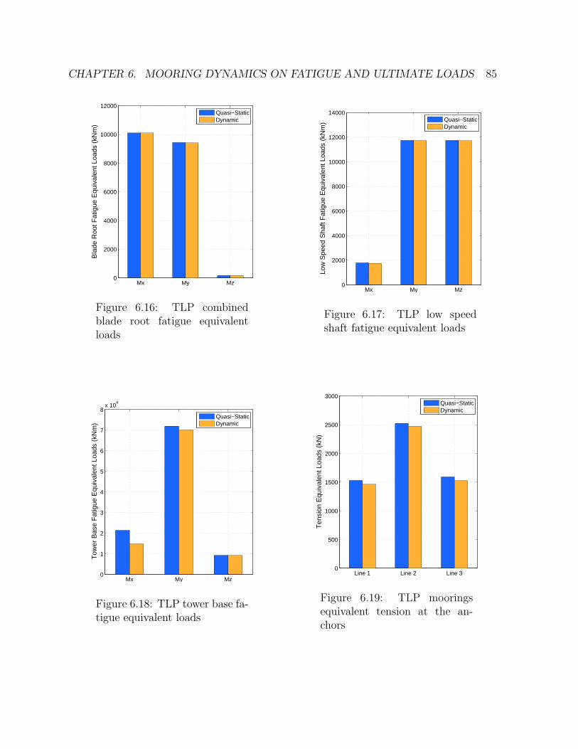
CHAPTER 6. MOORING DYNAMICS ON FATIGUE AND ULTIMATE LOADS 85
Mx My Mz0
2000
4000
6000
8000
10000
12000
Bla
de R
oot F
atig
ue E
quiv
alen
t Loa
ds (
kNm
)
Quasi−StaticDynamic
Figure 6.16: TLP combinedblade root fatigue equivalentloads
Mx My Mz0
2000
4000
6000
8000
10000
12000
14000
Low
Spe
ed S
haft
Fat
igue
Equ
ival
ent L
oads
(kN
m)
Quasi−StaticDynamic
Figure 6.17: TLP low speedshaft fatigue equivalent loads
Mx My Mz0
1
2
3
4
5
6
7
8x 10
4
Tow
er B
ase
Fat
igue
Equ
ival
ent L
oads
(kN
m)
Quasi−StaticDynamic
Figure 6.18: TLP tower base fa-tigue equivalent loads
Line 1 Line 2 Line 30
500
1000
1500
2000
2500
3000
Ten
sion
Equ
ival
ent L
oads
(kN
)
Quasi−StaticDynamic
Figure 6.19: TLP mooringsequivalent tension at the an-chors

CHAPTER 6. MOORING DYNAMICS ON FATIGUE AND ULTIMATE LOADS 86
6.5.4 Summary of the effect of mooring lines dynamics on thefatigue loads of the three platforms
In this Subsection, the relative differences between the loads computed using the quasi-staticand the dynamic moorings model are compared for the three platforms to identify in whichcomponents and platform designs the effect of the lines dynamics is more important. Apositive value in the differences means higher loads calculated using dynamic lines modeland a negative value means lower loads calculated by the dynamic model. The referencevalue for the calculation of the percentages of difference is the quasi-static.Figures 6.20 and 6.21 show that the effect of the lines dynamics only slightly affects theequivalent fatigue loads at the blade root and the shaft for any of the three platforms, withdifferences below 0.3% in the blade root and 2% in the shaft. Nevertheless, small differencesin fatigue loads of an element can have an impact on the design.The mooring lines dynamic model produces a decrease in the tower fatigue loads (Figure6.22) for the three platform designs. This decrease is higher for the component Mx of thetower base moment, in particular for the TLP platform (31%), being also important for thesemisubmersible (13%). The decrease in the My component is lower due to the effect ofthe rotor aerodynamic thrust: around 2% and 2.5% for the semisubmersible and the TLP,respectively. For the spar, the reduction in the tower base moment is very small due to thereduced influence of the mooring system on the rotations.Figure 6.23 shows that the effect of dynamics is very important on the line tension, reducingthe fatigue loads for the spar and the TLP due to the extra damping not captured by thequasi-static approach. For the spar, the decrease is around 8% for the upwind lines 2 and 3,and 2% for the downwind line. For the TLP the mooring approach is not so critical: usingthe dynamic model decreases less than 5% the equivalent tension in the upwind lines andaround 2% in the downwind line. For the semisubmersible platform, where the heave naturalfrequency is inside the wave spectrum, the effect of the mooring dynamics is different than inthe other two platforms. The excitation of the platform’s heave displacement produces highvelocities and accelerations in the lines increasing the loads due to the drag and inertia. Inthis case, the dynamic model provides 57% higher equivalent tension loads for the upwindline (line 2) with respect to the quasi-static, and between 25% - 30% for the downwind lines(lines 1 and 3).
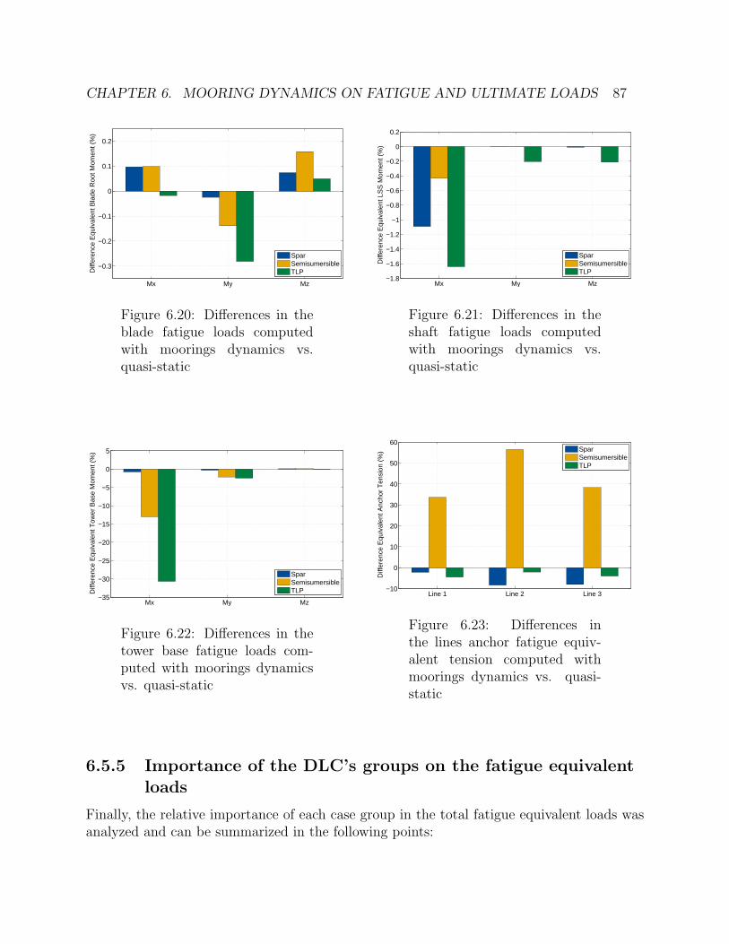
CHAPTER 6. MOORING DYNAMICS ON FATIGUE AND ULTIMATE LOADS 87
Mx My Mz
−0.3
−0.2
−0.1
0
0.1
0.2
Diff
eren
ce E
quiv
alen
t Bla
de R
oot M
omen
t (%
)
SparSemisumersibleTLP
Figure 6.20: Differences in theblade fatigue loads computedwith moorings dynamics vs.quasi-static
Mx My Mz−1.8
−1.6
−1.4
−1.2
−1
−0.8
−0.6
−0.4
−0.2
0
0.2
Diff
eren
ce E
quiv
alen
t LS
S M
omen
t (%
)
SparSemisumersibleTLP
Figure 6.21: Differences in theshaft fatigue loads computedwith moorings dynamics vs.quasi-static
Mx My Mz−35
−30
−25
−20
−15
−10
−5
0
5
Diff
eren
ce E
quiv
alen
t Tow
er B
ase
Mom
ent (
%)
SparSemisumersibleTLP
Figure 6.22: Differences in thetower base fatigue loads com-puted with moorings dynamicsvs. quasi-static
Line 1 Line 2 Line 3−10
0
10
20
30
40
50
60
Diff
eren
ce E
quiv
alen
t Anc
hor
Ten
sion
(%
)
SparSemisumersibleTLP
Figure 6.23: Differences inthe lines anchor fatigue equiv-alent tension computed withmoorings dynamics vs. quasi-static
6.5.5 Importance of the DLC’s groups on the fatigue equivalentloads
Finally, the relative importance of each case group in the total fatigue equivalent loads wasanalyzed and can be summarized in the following points:

CHAPTER 6. MOORING DYNAMICS ON FATIGUE AND ULTIMATE LOADS 88
• DLC 1.2 provides around 99% of the fatigue load for almost all the wind turbinecomponents in the three platforms. The only exception is the tower base load in theTLP, where DLC 6.4 contributes with 3-5% of the load. The importance of DLC 2.4and DLC 4.1 is neglectable.
• For the equivalent fatigue tension of the lines, the role of DLC 6.4 is higher than inthe wind turbine components, specially when dynamic mooring model is used. DLC2.4 and DLC 4.1 are also neglectable.
• For the spar, DLC 6.4 provides 6% of the fatigue load in the downwind line with thedynamic model, but less than 1% with the quasi-static.
• For the semisubmersible, if the dynamic model is used, DLC 6.4 contributes with 14%of the fatigue load in the two downwind lines and around 7% in the upwind line. Butif the quasi-static model is used, the contribution of DLC 6.4 is reduced to 3% for thedownwind lines and below 1% for the upwind.
• Finally, for the TLP, the relative importance of the DLC’s in the fatigue calculation issimilar for both mooring models; DLC 6.4 contributes with 6-7% of the total fatiguedamage in the downwind lines and 3.6% in the upwind line, no matter which model isused. The rest of the fatigue load is provided by DLC 1.2.
6.6 Impact of mooring lines dynamics on ultimate
loads
In this section, the ultimate loads are presented in bar diagrams, and at the top of each bar,the load case group providing each ultimate load is indicated for information. A discussionon the importance of the different load case groups is given at the end of the section.
6.6.1 Spar ultimate loads
The effect of the mooring line dynamics on the ultimate loads of the wind turbine componentsis very low for the spar, see Figures 6.24 (blade root), 6.25 (shaft) and 6.26 (tower base).The differences on the modelling of the lines does not affect the platform motions in roll andpitch due to the position of the fairleads close to the platform rotation center.The lines extreme tensions are sensitive to the lines model, as it is appreciated in Figure6.27. The extreme environmental conditions defined for the simulation of the ultimate loadscases induce higher velocities and accelerations to the platform than in the fatigue cases.This leads to higher loads in the lines when the dynamic model is used, due to the drag and

CHAPTER 6. MOORING DYNAMICS ON FATIGUE AND ULTIMATE LOADS 89
the inertial effects. The maximum tension of the lines is increased by 11% for line 1 and by15% for the lines 2 and 3. The minimum tensions are also decreased by the dynamic model.
−2
−1.5
−1
−0.5
0
0.5
1
1.5
2
2.5
3
x 104
dlc6
1
dlc6
2
dlc1
6
dlc1
6
dlc6
2
dlc6
2
dlc6
1
dlc6
2
dlc1
6
dlc1
6
dlc6
2
dlc6
2
Max
Mx
Min
Mx
Max
My
Min
My
Max
Mz
Min
Mz
Bla
de R
oot M
omen
tum
(kN
m)
Quasi−StaticDynamic
Figure 6.24: Ultimate loads at blade root for the spar platform
−2.5
−2
−1.5
−1
−0.5
0
0.5
1
1.5
2
2.5
x 104
dlc5
1
dlc5
1
dlc1
3
dlc1
3
dlc1
6
dlc1
6
dlc5
1
dlc5
1
dlc1
3
dlc1
3
dlc1
6
dlc1
6
Max
Mx
Min
Mx
Max
My
Min
My
Max
Mz
Min
Mz
Ulti
mat
e Lo
w S
peed
Sha
ft M
omen
tum
(kN
m)
Quasi−StaticDynamic
Figure 6.25: Ultimate loads at the low speed shaft for the spar platform
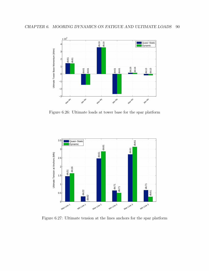
CHAPTER 6. MOORING DYNAMICS ON FATIGUE AND ULTIMATE LOADS 90
−3
−2
−1
0
1
2
3
4
x 105
dlc6
1
dlc6
1
dlc1
6
dlc6
1
dlc1
6
dlc1
3
dlc6
1
dlc6
1
dlc1
6
dlc6
1
dlc1
6
dlc1
3
Max
Mx
Min
Mx
Max
My
Min
My
Max
Mz
Min
Mz
Ulti
mat
e T
ower
Bas
e M
omen
tum
(kN
m)
Quasi−StaticDynamic
Figure 6.26: Ultimate loads at tower base for the spar platform
0
0.5
1
1.5
2
2.5
3
3.5
dlc5
1
dlc2
2
dlc6
1
dlc7
1
dlc6
1
dlc7
1
dlc1
6
dlc6
2
dlc6
1
dlc7
1
dlc6
1
dlc6
1
Ulti
mat
e T
ensi
on a
t Anc
hors
(M
N)
Max Line 1
Min Line 1
Max Line 2
Min Line 2
Max Line 3
Min Line 3
Quasi−StaticDynamic
Figure 6.27: Ultimate tension at the lines anchors for the spar platform
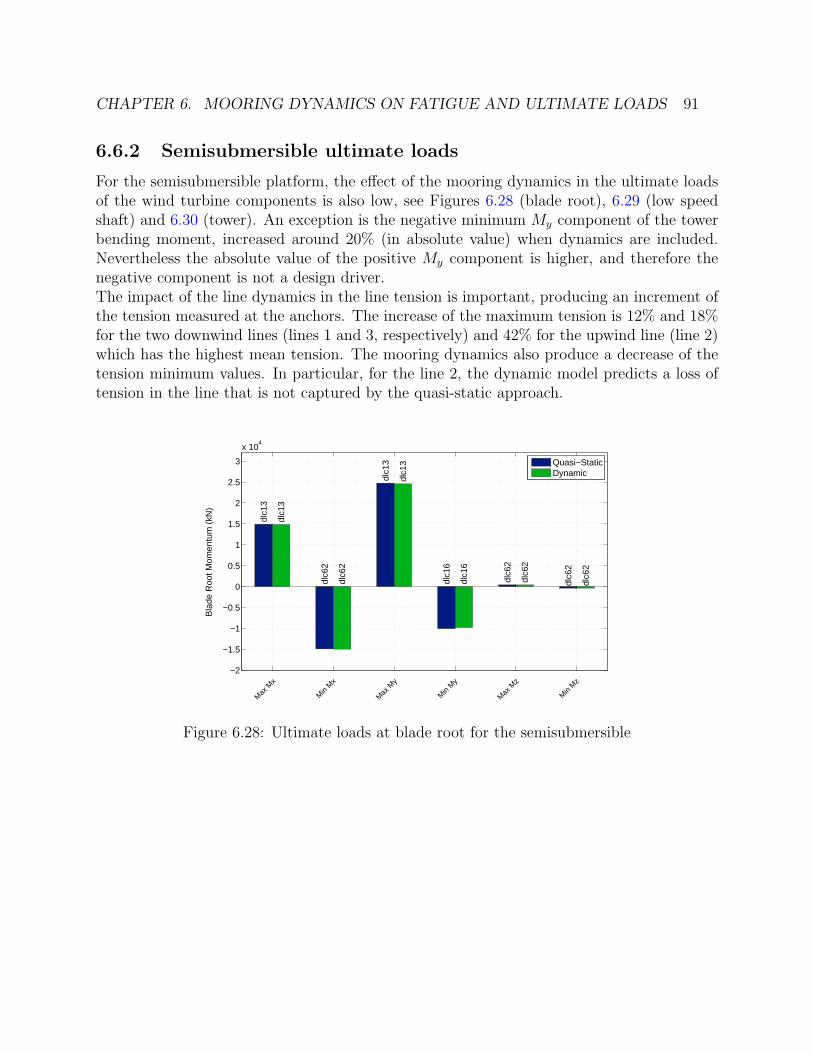
CHAPTER 6. MOORING DYNAMICS ON FATIGUE AND ULTIMATE LOADS 91
6.6.2 Semisubmersible ultimate loads
For the semisubmersible platform, the effect of the mooring dynamics in the ultimate loadsof the wind turbine components is also low, see Figures 6.28 (blade root), 6.29 (low speedshaft) and 6.30 (tower). An exception is the negative minimum My component of the towerbending moment, increased around 20% (in absolute value) when dynamics are included.Nevertheless the absolute value of the positive My component is higher, and therefore thenegative component is not a design driver.The impact of the line dynamics in the line tension is important, producing an increment ofthe tension measured at the anchors. The increase of the maximum tension is 12% and 18%for the two downwind lines (lines 1 and 3, respectively) and 42% for the upwind line (line 2)which has the highest mean tension. The mooring dynamics also produce a decrease of thetension minimum values. In particular, for the line 2, the dynamic model predicts a loss oftension in the line that is not captured by the quasi-static approach.
−2
−1.5
−1
−0.5
0
0.5
1
1.5
2
2.5
3
x 104
dlc1
3
dlc6
2
dlc1
3
dlc1
6
dlc6
2
dlc6
2
dlc1
3
dlc6
2
dlc1
3
dlc1
6
dlc6
2
dlc6
2
Max
Mx
Min
Mx
Max
My
Min
My
Max
Mz
Min
Mz
Bla
de R
oot M
omen
tum
(kN
)
Quasi−StaticDynamic
Figure 6.28: Ultimate loads at blade root for the semisubmersible
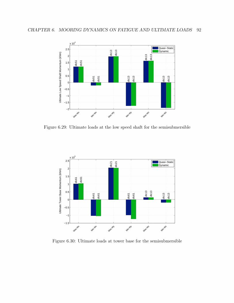
CHAPTER 6. MOORING DYNAMICS ON FATIGUE AND ULTIMATE LOADS 92
−2
−1.5
−1
−0.5
0
0.5
1
1.5
2
2.5
x 104
dlc5
1
dlc5
1
dlc1
3
dlc1
3
dlc1
3
dlc1
3
dlc5
1
dlc5
1
dlc1
3
dlc1
3
dlc1
3
dlc1
3
Max
Mx
Min
Mx
Max
My
Min
My
Max
Mz
Min
Mz
Ulti
mat
e Lo
w S
peed
Sha
ft M
omen
tum
(kN
m)
Quasi−StaticDynamic
Figure 6.29: Ultimate loads at the low speed shaft for the semisubmersible
−1.5
−1
−0.5
0
0.5
1
1.5
2
2.5x 10
5
dlc6
1
dlc6
1
dlc2
1
dlc6
1
dlc1
3
dlc1
3
dlc6
1
dlc6
1
dlc2
1
dlc6
1
dlc1
3
dlc1
3
Max
Mx
Min
Mx
Max
My
Min
My
Max
Mz
Min
Mz
Ulti
mat
e T
ower
Bas
e M
omen
tum
(kN
m)
Quasi−StaticDynamic
Figure 6.30: Ultimate loads at tower base for the semisubmersible
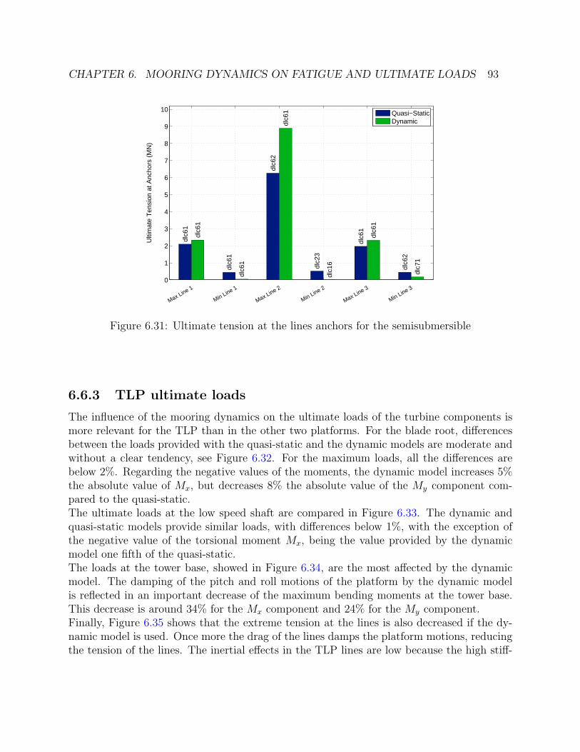
CHAPTER 6. MOORING DYNAMICS ON FATIGUE AND ULTIMATE LOADS 93
0
1
2
3
4
5
6
7
8
9
10
dlc6
1
dlc6
1
dlc6
2
dlc2
3
dlc6
1
dlc6
2
dlc6
1
dlc6
1
dlc6
1
dlc1
6
dlc6
1
dlc7
1
Ulti
mat
e T
ensi
on a
t Anc
hors
(M
N)
Max Line 1
Min Line 1
Max Line 2
Min Line 2
Max Line 3
Min Line 3
Quasi−StaticDynamic
Figure 6.31: Ultimate tension at the lines anchors for the semisubmersible
6.6.3 TLP ultimate loads
The influence of the mooring dynamics on the ultimate loads of the turbine components ismore relevant for the TLP than in the other two platforms. For the blade root, differencesbetween the loads provided with the quasi-static and the dynamic models are moderate andwithout a clear tendency, see Figure 6.32. For the maximum loads, all the differences arebelow 2%. Regarding the negative values of the moments, the dynamic model increases 5%the absolute value of Mx, but decreases 8% the absolute value of the My component com-pared to the quasi-static.The ultimate loads at the low speed shaft are compared in Figure 6.33. The dynamic andquasi-static models provide similar loads, with differences below 1%, with the exception ofthe negative value of the torsional moment Mx, being the value provided by the dynamicmodel one fifth of the quasi-static.The loads at the tower base, showed in Figure 6.34, are the most affected by the dynamicmodel. The damping of the pitch and roll motions of the platform by the dynamic modelis reflected in an important decrease of the maximum bending moments at the tower base.This decrease is around 34% for the Mx component and 24% for the My component.Finally, Figure 6.35 shows that the extreme tension at the lines is also decreased if the dy-namic model is used. Once more the drag of the lines damps the platform motions, reducingthe tension of the lines. The inertial effects in the TLP lines are low because the high stiff-
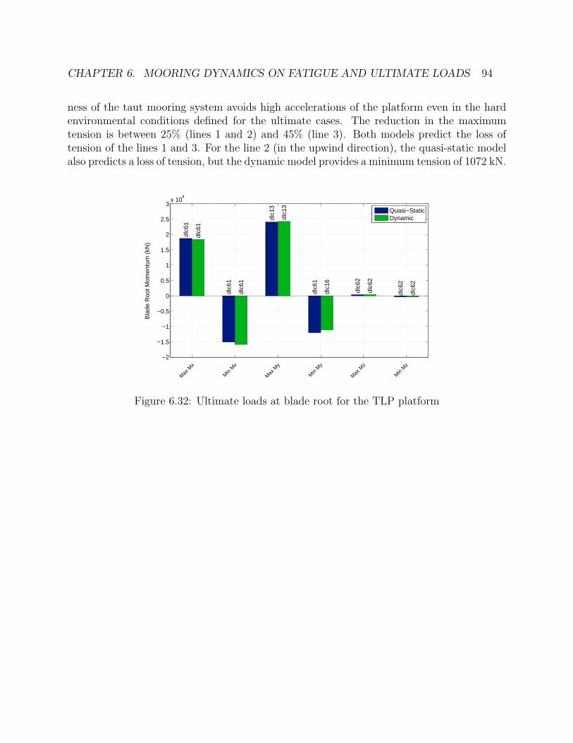
CHAPTER 6. MOORING DYNAMICS ON FATIGUE AND ULTIMATE LOADS 94
ness of the taut mooring system avoids high accelerations of the platform even in the hardenvironmental conditions defined for the ultimate cases. The reduction in the maximumtension is between 25% (lines 1 and 2) and 45% (line 3). Both models predict the loss oftension of the lines 1 and 3. For the line 2 (in the upwind direction), the quasi-static modelalso predicts a loss of tension, but the dynamic model provides a minimum tension of 1072 kN.
−2
−1.5
−1
−0.5
0
0.5
1
1.5
2
2.5
3x 10
4
dlc6
1
dlc6
1
dlc1
3
dlc6
1
dlc6
2
dlc6
2
dlc6
1
dlc6
1
dlc1
3
dlc1
6
dlc6
2
dlc6
2
Max
Mx
Min
Mx
Max
My
Min
My
Max
Mz
Min
Mz
Bla
de R
oot M
omen
tum
(kN
)
Quasi−StaticDynamic
Figure 6.32: Ultimate loads at blade root for the TLP platform
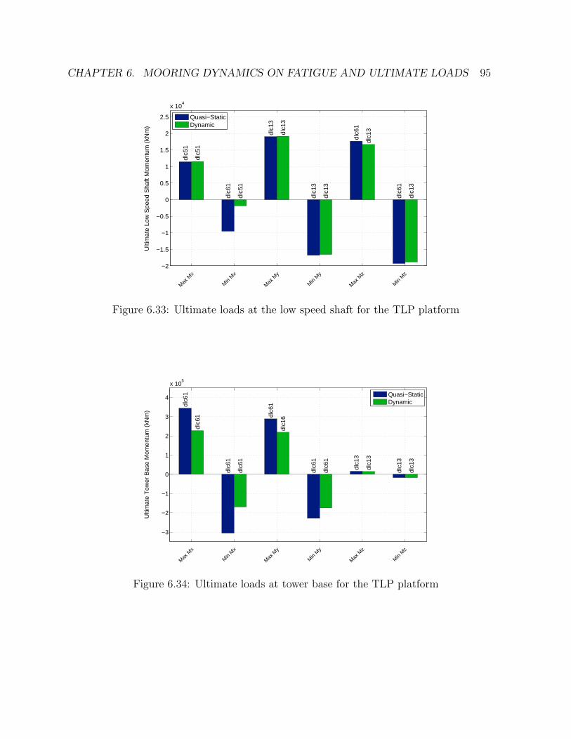
CHAPTER 6. MOORING DYNAMICS ON FATIGUE AND ULTIMATE LOADS 95
−2
−1.5
−1
−0.5
0
0.5
1
1.5
2
2.5
x 104
dlc5
1
dlc6
1
dlc1
3
dlc1
3
dlc6
1
dlc6
1
dlc5
1
dlc5
1
dlc1
3
dlc1
3
dlc1
3
dlc1
3
Max
Mx
Min
Mx
Max
My
Min
My
Max
Mz
Min
Mz
Ulti
mat
e Lo
w S
peed
Sha
ft M
omen
tum
(kN
m)
Quasi−StaticDynamic
Figure 6.33: Ultimate loads at the low speed shaft for the TLP platform
−3
−2
−1
0
1
2
3
4
x 105
dlc6
1
dlc6
1
dlc6
1
dlc6
1
dlc1
3
dlc1
3
dlc6
1
dlc6
1
dlc1
6
dlc6
1
dlc1
3
dlc1
3
Max
Mx
Min
Mx
Max
My
Min
My
Max
Mz
Min
Mz
Ulti
mat
e T
ower
Bas
e M
omen
tum
(kN
m)
Quasi−StaticDynamic
Figure 6.34: Ultimate loads at tower base for the TLP platform
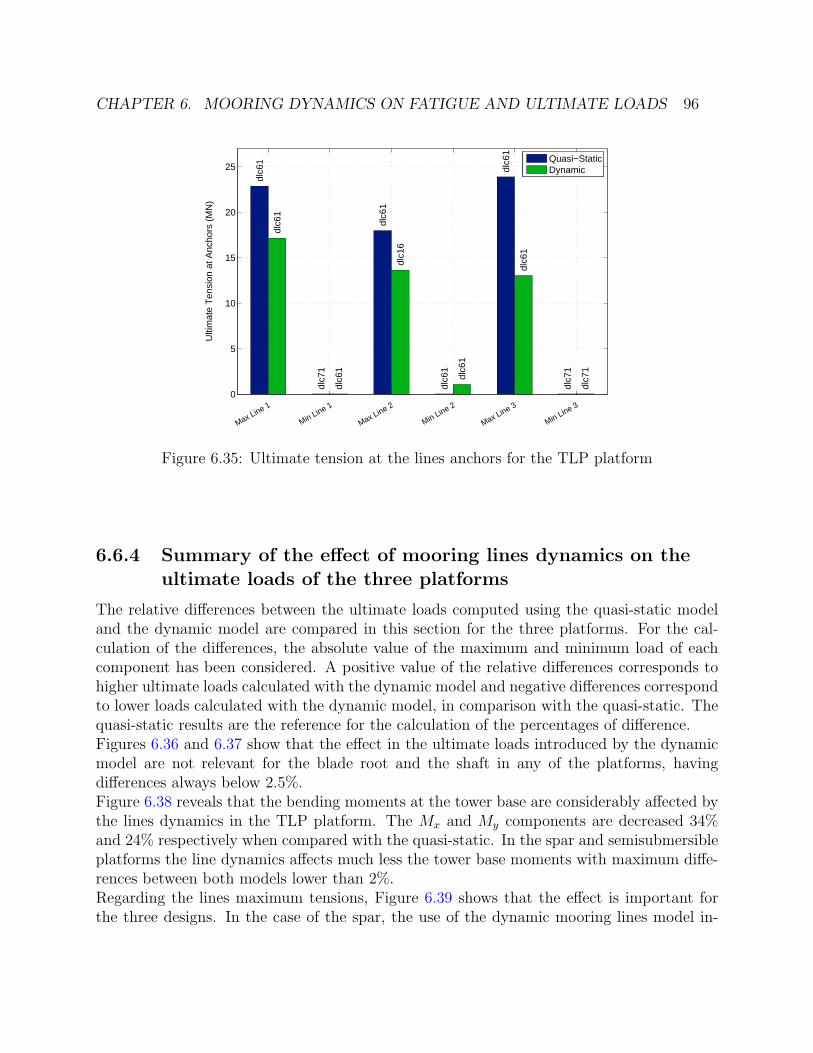
CHAPTER 6. MOORING DYNAMICS ON FATIGUE AND ULTIMATE LOADS 96
0
5
10
15
20
25
dlc6
1
dlc7
1
dlc6
1
dlc6
1
dlc6
1
dlc7
1
dlc6
1
dlc6
1
dlc1
6
dlc6
1
dlc6
1
dlc7
1
Ulti
mat
e T
ensi
on a
t Anc
hors
(M
N)
Max Line 1
Min Line 1
Max Line 2
Min Line 2
Max Line 3
Min Line 3
Quasi−StaticDynamic
Figure 6.35: Ultimate tension at the lines anchors for the TLP platform
6.6.4 Summary of the effect of mooring lines dynamics on theultimate loads of the three platforms
The relative differences between the ultimate loads computed using the quasi-static modeland the dynamic model are compared in this section for the three platforms. For the cal-culation of the differences, the absolute value of the maximum and minimum load of eachcomponent has been considered. A positive value of the relative differences corresponds tohigher ultimate loads calculated with the dynamic model and negative differences correspondto lower loads calculated with the dynamic model, in comparison with the quasi-static. Thequasi-static results are the reference for the calculation of the percentages of difference.Figures 6.36 and 6.37 show that the effect in the ultimate loads introduced by the dynamicmodel are not relevant for the blade root and the shaft in any of the platforms, havingdifferences always below 2.5%.Figure 6.38 reveals that the bending moments at the tower base are considerably affected bythe lines dynamics in the TLP platform. The Mx and My components are decreased 34%and 24% respectively when compared with the quasi-static. In the spar and semisubmersibleplatforms the line dynamics affects much less the tower base moments with maximum diffe-rences between both models lower than 2%.Regarding the lines maximum tensions, Figure 6.39 shows that the effect is important forthe three designs. In the case of the spar, the use of the dynamic mooring lines model in-
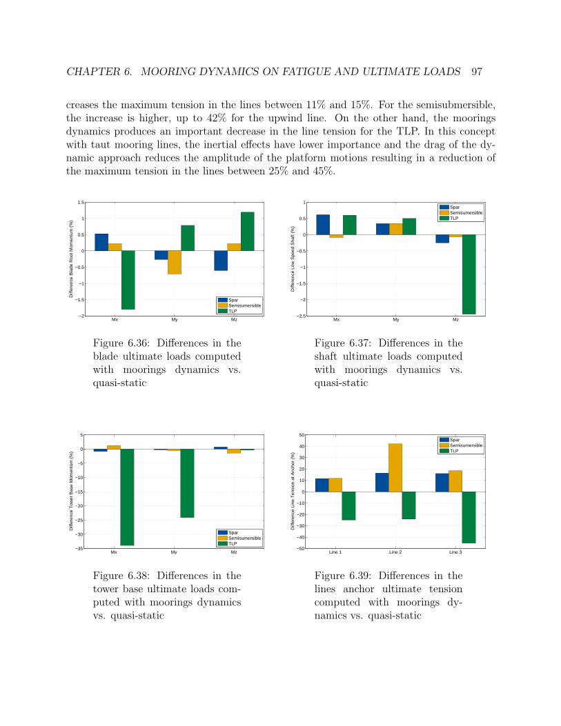
CHAPTER 6. MOORING DYNAMICS ON FATIGUE AND ULTIMATE LOADS 97
creases the maximum tension in the lines between 11% and 15%. For the semisubmersible,the increase is higher, up to 42% for the upwind line. On the other hand, the mooringsdynamics produces an important decrease in the line tension for the TLP. In this conceptwith taut mooring lines, the inertial effects have lower importance and the drag of the dy-namic approach reduces the amplitude of the platform motions resulting in a reduction ofthe maximum tension in the lines between 25% and 45%.
Mx My Mz−2
−1.5
−1
−0.5
0
0.5
1
1.5
Diff
eren
ce B
lade
Roo
t Mom
entu
m (
%)
SparSemisumersibleTLP
Figure 6.36: Differences in theblade ultimate loads computedwith moorings dynamics vs.quasi-static
Mx My Mz−2.5
−2
−1.5
−1
−0.5
0
0.5
1
Diff
eren
ce L
ow S
peed
Sha
ft (%
)
SparSemisumersibleTLP
Figure 6.37: Differences in theshaft ultimate loads computedwith moorings dynamics vs.quasi-static
Mx My Mz−35
−30
−25
−20
−15
−10
−5
0
5
Diff
eren
ce T
ower
Bas
e M
omen
tum
(%
)
SparSemisumersibleTLP
Figure 6.38: Differences in thetower base ultimate loads com-puted with moorings dynamicsvs. quasi-static
Line 1 Line 2 Line 3−50
−40
−30
−20
−10
0
10
20
30
40
50
Diff
eren
ce L
ine
Ten
sion
at A
ncho
r (%
)
SparSemisumersibleTLP
Figure 6.39: Differences in thelines anchor ultimate tensioncomputed with moorings dy-namics vs. quasi-static
CHAPTER 6. MOORING DYNAMICS ON FATIGUE AND ULTIMATE LOADS 98
6.6.5 Importance of the DLC’s groups on the ultimate loads
An overview of the importance of the load case groups in the ultimate loads is given inthis subsection, although a deeper analysis will be done in future work. The group of casesproviding each ultimate load was indicated in the plots of the ultimate loads (Figures 6.24to 6.35).
• The group of cases DLC 6.1 is driving a large number of extreme loads. It alwaysdetermines the maximum tension at the anchor lines for all the platforms, with the ex-ception of the maximum tension at the semisubmersible with the quasi-static mooringmodel, given by DLC 6.2. In addition, DLC 6.1 determines the maximum Mx com-ponent of the blade root moment for the spar and the TLP and the maximum Mx
component of the tower base moment for the three platforms.
• DLC 1.3 has also great importance, marking the extreme shaft bending moment in thethree platform concepts and the blade root bending moment for the semisubmersible(Mx and My components) and the TLP (My component). It also provides the extremetorsional moment of the tower for the three platforms.
• DLC 1.6 is particularly relevant for the spar platform, where it is responsible of theextreme loads for the blade My, the shaft Mz and the tower My components of thebending moments. For the TLP it also determines the maximum tower base My mo-ment with the dynamic model.
• DLC 5.1 provides the maximum torsional moment at the shaft for all the platformdesigns.
• Finally, DLC 2.1 provides the maximum My component of the tower base moment forthe semisubmersible.
6.7 Concluding remarks
A comprehensive study on the influence of mooring line dynamics on the calculation of windturbine loads following the standard certification requirements for the wind energy industryhas been presented.Three different platform designs (spar, semisubmersible and TLP) were studied to characte-rize the effect of the mooring dynamics on each concept. The loads were computed followingthe methodology defined by the IEC 61400-3 Edition 1 guideline, which implied the com-putation and postprocessing of more than 20,000 cases. The fatigue and ultimate loadsobtained for each platform design using a quasi-static and a dynamic moorings model werecompared.The impact of moorings dynamics in the results provided by integrated simulation codes
CHAPTER 6. MOORING DYNAMICS ON FATIGUE AND ULTIMATE LOADS 99
depends on the topology of the floating platform and the component considered.In general, the influence of mooring dynamics in both fatigue and ultimate loads increasesas elements located closer to the platform are evaluated; the blade and the shaft loads areonly slightly modified by the mooring dynamics in all the platform designs, the tower baseloads can be significantly affected depending on the platform concept, and the mooring linestensions strongly depend on the lines dynamics both in fatigue and extreme loads in all theplatform concepts evaluated.The equivalent fatigue tension at the anchors of the three platforms is impacted by themoorings dynamics, but the effect depends on the platform considered. For the semisub-mersible, with the heave natural period inside the wave spectrum, dynamics increase theequivalent tension up to 57%. For the spar and the TLP, the equivalent tensions are mod-erately decreased (up to 8%).For the spar, the effect of mooring dynamics on the fatigue of the wind turbine components(blades, shaft and tower) is low due to the low influence of the mooring system on the pitchand roll motions. For the semisubmersible and the TLP, moorings dynamics introduce a sig-nificant decrease in the fatigue of the wind turbine components, in particular for the tower.Regarding ultimate loads, mooring dynamics cannot be neglected for the calculation of theextreme line tensions in any of the three platforms studied. Including mooring dynamics inthe integrated simulations can have diverse effects on the extreme line tensions dependingon the platform type, with an increase (spar and semisubmersible) or decrease (TLP) of upto 40% with respect to the quasi-static.Mooring dynamics are definitely needed for the calculation of the tower base ultimate loadsin the TLP design, where the extreme moments are decreased between 24% and 34%. Forthe other platforms and wind turbine elements, the effect on the ultimate loads is much morelimited.As a final remark, this study reveals that mooring dynamics has the greatest impact in thecomputation of:
• Fatigue equivalent tensions and ultimate tensions of the mooring lines in any platformconfiguration.
• In particular, fatigue equivalent tensions of the moorings for the semisubmersible, withone natural frequency inside the wave spectrum.
• Fatigue and ultimate loads of the components of the wind turbine supported by theTLP.
• Tower base fatigue for platforms with fairleads located far from the platform center,such as the semisubmersible and the TLP.

100
Chapter 7
Conclusions and future lines ofresearch
7.1 Conclusions
The work performed in this research has consisted on the building of a dynamic mooring linessimulation code that has been coupled with an integrated code for the simulation of floatingwind turbines and verified in an international benchmark (OC4). Afterwards, the dynamicmooring line code has been experimentally validated with experimental measurements of asubmerged chain in a water basin. Once validated, the new integrated tool has been used toevaluate the effect of mooring dynamics on the computation of ultimate and fatigue loadsfor the main existing topologies of floating wind turbines. This evaluation has provided in-dications of great interest for the designers to determine the required level of complexity onthe mooring system modelling for integrated floating wind turbine simulations, dependingon the type of platform, the simulation case and the expected results.The dynamic mooring line code developed, called OPASS, is based on a finite element model.The computational cost has been reduced using a lumped mass formulation. The efficiencyof this approach to include mooring dynamics in integrated floating wind turbine codes hasbeen demonstrated: the OPASS model coupled with FAST has been used in the last part ofthis research to simulate the complete set of load cases required by the IEC 61400-3 guidelinefor the three main floating wind turbine topologies.A test campaign for the validation of the mooring lines dynamic code was performed atthe Ecole Centrale de Nantes (ECN) wave tank. An original testing setup for the mooringdynamics has been designed consisting on the installation of a submerged chain in a waterbasin, with one end anchored at the bottom of the basin and the suspension point beingexcited with harmonic horizontal motions of different frequencies. The tension of the line atthe fairlead was measured using a load cell. It is remarkable that the trajectories of markerslocated at different positions along the length of the line were also measured using a systemof submerged cameras, resulting in a very detailed dataset of results.

CHAPTER 7. CONCLUSIONS AND FUTURE LINES OF RESEARCH 101
The accuracy of the dynamic model has been evaluated against the experimental data ob-tained at the water tank tests with good results. Two configurations of the chain have beenstudied, with different tension levels. In the static cases, both the shape of the line andthe tension at the suspension point compare very well between the computations and theexperiments, presenting negligible discrepancies.The dynamic experimental results include different dynamic conditions as harmonic response,loss of tension and snap loads, which is a highly dynamic case, challenging from the pointof view of simulation, that has to be considered when validating a dynamic mooring model.In all these conditions, the code is able to predict the motion of the markers at differentchain positions accurately and also the tension at the fairlead is captured with precision, de-monstrating that the drag coefficients for the chain simulations, that have been chosen fromguidelines, in general represent accurately the hydrodynamic loads. The highest disagree-ment appears in the cases with the highest frequency of the excitation motion, where themaximum tension is overpredicted by the code by around 4.5%. These differences, althoughare small, could be caused by a dependency of the drag coefficients with the frequency ofthe motions and to the fact that the values from guidelines could be tuned for the cases withlow excitation frequencies. According to the sensitivity analysis of the tension to changes inthe drag coefficients, a slight decrease of the drag as the frequency of the excitation motionincreases can provide a better agreement with the tension experimental measurements.In the cases with the highest pretension level and highest excitation frequency, the line totallyloses the tension during part of the fairlead excitation period and the simulation results areparticularly sensitive to the cable-seabed interaction model. In this situation, the modellingof the seabed friction must be considered because it plays an important role avoiding theslide of the line nodes on the seabed during the period with no tension in the line. This slideof the nodes, that is not present in the experiments due to the friction of the chain with thebottom of the basin, can greatly affect the line dynamics after several periods of fairlead ex-citation and has to be avoided using an adequate friction coefficient to have accurate results.In the cases where the excitation frequency is lower and the lines does not lose tension, theeffect of the seabed-line friction coefficient is not significant.An important contribution of this research is the characterization of the effect that themooring dynamics have on the computation of the certification loads for the three main con-cepts of platform designs (spar, semisubmersible and TLP). The fatigue and ultimate loadsobtained for each platform design using a quasi-static and a dynamic moorings model werecompared. These loads were computed according to the IEC 61400-3 Edition 1 guideline,which implied the computation and postprocessing of more than 20,000 cases.From this study, it can be concluded that in general, the influence of mooring dynamicsin both fatigue and ultimate loads increases as elements located closer to the platform areevaluated; the blade and the shaft loads are only slightly modified by the mooring dynamicsin all the platform designs, the tower base loads can be significantly affected depending onthe platform concept, and the mooring lines tensions strongly depend on the lines dynamicsboth in fatigue and extreme loads in all the platform concepts evaluated.
CHAPTER 7. CONCLUSIONS AND FUTURE LINES OF RESEARCH 102
In particular, the computation of the equivalent fatigue tension of the lines is impacted bythe moorings dynamics for the three platforms studied, but the effect is more pronounced forthe semisubmersible, that presents the heave natural period inside the wave spectrum. Forthis platform concept, the dynamic moorings model increases the equivalent tension up to57% and for the other two platforms, equivalent fatigue tensions are moderately decreased.The equivalent fatigue loads at the wind turbine elements, specially at the tower base, aresignificantly decreased by the mooring dynamics.Relating the calculation of the ultimate loads, the consideration of mooring dynamics in theintegrated simulations can have diverse effects on the extreme line tensions depending onthe platform type, with an increase (spar and semisubmersible) or decrease (TLP) of up to40% with respect to the quasi-static. In addition, mooring dynamics decrease the tower baseultimate loads for the TLP design between 24% and 34%. For the other platforms the effecton the tower ultimate loads is much more limited.The study of the impact of mooring dynamics on the computation of fatigue and ultimateloads according to the certification guidelines has shown that dynamic models should beincluded for the computation of:
• Fatigue equivalent tensions and ultimate tensions of the mooring lines in any platformconfiguration.
• In particular, fatigue equivalent tensions of the moorings for the semisubmersible designstudied, that presents the heave natural frequency inside the wave spectrum.
• Fatigue and ultimate loads of the components of the wind turbine supported by theTLP.
• Tower base fatigue loads for platforms with fairleads located far from the platformcenter, such as the semisubmersible and the TLP.
7.2 Future lines of research
The field of research of this dissertation is far from being exhausted and present many po-tential topics to be investigated in the future, such as the inclusion of new capabilities in themoorings simulation model, the increase of the computational efficiency, the improvementof the numerical robustness of the code, the better characterization of parameters used incomputational models and a further identification of the importance of dynamic effects underdifferent conditions.The simulation tool developed in this work is applicable to lines with no bending and torsionstiffness as chains. An upgrade of the code to include bending and torsion will allow to modellines where these effects have importance, as synthetic moorings and also the electrical cablesthat evacuate the energy produced by the wind turbine. Additionally, the accurate mode-lling of synthetic lines requires the implementation of more advance and specific internal
CHAPTER 7. CONCLUSIONS AND FUTURE LINES OF RESEARCH 103
damping models, where investigation effort is required. Many mooring designs, in particularfor high sea depths, include hybrid lines composed of different materials as chain, wire orropes. Future upgrades of the code should consider these type of designs. The line seabedcontact model is another aspect that can be improved in the future. The approach basedon springs to introduce the vertical reaction force in the nodes in contact with the seabedusually requires a tuning to ensure numerical stability. More robust seabed contact modelscould be developed using Lagrangian mechanics principles or other equivalent methods.The vortex induced vibrations (VIV) at moorings in tension can be an important phenomenain the design of TLP’s. This type of platforms can present natural frequencies that could beexcited by this effect. More research on the influence of VIV in the design of wind turbineswith TLP substructures and further development of analysis tools are still required. For theanalysis of VIV, the dynamic mooring line model has to be coupled with a computation ofthe whole fluid field that surrounds the line. That would be a hydrodynamic model morecomplex than the Morison approach used in this research due to its computational efficiency.There are also some aspects of the methods for the numerical integration of the equationsof motion with potential to increase the computational efficiency. The implementation of anstiff time integrator as the Newmark-β method [81] could significantly increment the simu-lation time step reducing the simulation cost. In addition, the assessment of loose versustight schemes for the coupling of mooring codes with floating platforms integrated simulationcodes is another open research line.An experimental characterization of the dependency of the chain’s tangential and normaldrag coefficients with the excitation frequency would be beneficial to increase the accuracyof simulations, in particular when high frequency motions are present.Relating the importance of mooring lines dynamics on the computation of loads for floatingwind turbines, the comparative analysis performed in this study for three different platformswas performed at the same water depth. The influence of the sea depth on the importance ofthe mooring dynamics for the simulations was not explored and it is probably an interestingaspect with implications on the modelling of floating wind turbines.Finally, many of the differences introduced by the mooring dynamics on the wind turbinecomponent loads are caused by the drag of the lines. A quasi-static model for the mooringlines combined with an additional damping matrix equivalent to the global damping intro-duced on the platform degrees of freedom by the mooring system could provide acceptableresults for the motions of the platform with low computational cost. The accuracy of thisapproach should be evaluated. Nevertheless, the effect of the mooring dynamics on the linesthemselves would not be captured.
104
Bibliography
[1] 2014 Half Year Report. Technical Report. World Wind Energy Association (WWEA),2014.
[2] Aamo, O.M. and Fossen, T.I. “Finite Element Modelling of Mooring Lines”. In:Math-ematics and Computers in Simulation 53 (1976), pp. 415–422. doi: 10.1016/S0378-4754(00)00235-4.
[3] Abedi, H., Davidson, L. and Voutsinas, S. “Development of Free Vortex Wake Methodfor Aerodynamic Loads on Rotor Blades”. In: EWEA 2014. Barcelona, Spain, 2014.
[4] AeroDyn Theory Manual. Technical Report TP-500-36881. Golden, Colorado, USA:NREL, 2005.
[5] Arapogianni, A., Genachte, A.B., Manzanas, R., Pascual, P., Castell, D., Rodriguez,A., Korbijn, J., Bolleman, N.C.F., Huera-Huarte, F.J., Schuon, F., Ugarte, A., Sand-berg, J., de Laleu, V., Maciel, J., Tunbjer, A., Roth, R., de la Gueriviere, P., Coulombeau,P., Jedrec, S., Philippe, C., Voutsinas, S., Weinstein, A., Vita, L., Byklum, E., Hur-ley, W.L. and Grubel, H. Deep Water - The Next Steps for Offshore Wind Energy.Technical Report. European Wind Energy Association (EWEA), July 2013.
[6] Arapogianni, A., Moccia, J., Williams, D. and Phillips, J. Wind in our Sails. TheComing of Europe’s Offshore Wind Energy Industry. 2011.
[7] ARIANE7 Theoretical Manual. Bureau Veritas. July 2011.
[8] Azcona, J. and Nygaard, T.A. “Mooring Line Dynamics Experiments and Computa-tions. Effects on Floating Wind Turbine Fatigue Life and Extreme Loads”. In: EERADeepWind’2016, 13th DeepSea Offshore Wind R&D Conference. Trondheim, Norway,2016.
[9] Azcona, J., Bekiropoulos, D., Bredmose, H., Heilskov, N.F., Krieger, A., Lutz, T.,Manjock, A., Manolas, D., Matha, D., Meister, K., Pereira, R., Rønby, J., SandnerF. and Voutsinas, S. State-of-the-art and implementation of design tools for floatingstructures. Deliverable 4.21. INNWIND.EU, 2013.
BIBLIOGRAPHY 105
[10] Azcona, J., Munduate, X., Gonzalez, L. and Nygaard, T.A. “Experimental Validationof a Dynamic Mooring Lines Code with Tension and Motion Measurements of aSubmerged Chain”. In: Ocean Engineering 129(2017) (2016), pp. 415–427. doi: 10.1016/j.oceaneng.2016.10.051.
[11] Azcona, J., Munduate, X., Merino, D. and Nygaard, T.A. “Dynamic Simulation ofMooring Lines for FloatingWind Turbines”. In: EAWE PhD Seminar on Wind Energyin Europe. Delft, The Netherlands, 2011.
[12] Azcona, J., Munduate, X., Nygaard, T.A. and Merino, D. “Development of OPASSCode for Dynamic Simulation of Mooring Lines in Contact with Seabed”. In: EWEAOffshore 2011. Amsterdam, The Netherlands, 2011.
[13] Azcona, J., Palacio, D., Munduate, X., Gonzalez, L. and Nygaard, T.A. “Impact ofMooring Dynamics on the Fatigue and Ultimate Loads of Three Offshore FloatingWind Turbines Computed with IEC 61400-3 Guideline”. In: Wind Energy (2016).doi: 10.1002/we.2064.
[14] Bae, Y.H. Development of a Dynamic Mooring Module: FEAM for FAST v8. Tech.rep. Texas A&M University, 2014.
[15] Bayati, I., Jonkman, J.M., Robertson, A. and Platt, A. “The Effects of Second-OrderHydrodynamics on a Semisubmersible Floating Offshore Wind Turbine”. In: Journalof Physics: Conference Series 524 (2014). doi: 10.1088/1742-6596/524/1/012094.
[16] Bladed Theory Manual Version 4.0. GL Garrad Hassan. Oct. 2010.
[17] Bossanyi, E., Burton, T. and Sharpe, D. Wind Energy Handbook. John Wiley andSons, 2001.
[18] Bureau Veritas. NR 493 R02 E. Classification of Mooring Systems for PermanentOffshore Units. 2002.
[19] Corbetta, G., Mbistrova, A., Ho, A., Guillet, J. and Pineda, I. The European OffshoreWind Industry - Key Trends and Statistics 2014. Technical Report. European WindEnergy Association (EWEA), 2015.
[20] Corbetta, G., Pineda, I. and Wilkes, J. Wind in Power - 2014 European Statistics.Technical Report. European Wind Energy Association (EWEA), February 2015.
[21] Couch, A.T. and Conte, J.P. “Field Verification of Linear and Nonlinear, Hybrid WaveModels for Offshore Tower Response Prediction”. In: Journal of Offshore Mechanicsand Arctic Engineering 119 (3) (1997), pp. 158–165.
[22] De Vaal, J.B. and Nygaard, T.A. 3DFloat User Manual. Report IFE/KR/E-2015-001.Institute for Energy Technology. Norway, 2015.
[23] Dean R.G. “Stream Function Representation of Non-Linear Ocean Waves”. In: Jour-nal of Geophysical Research 70 (1965), pp. 4561–4572. doi: 10.1029/JZ070i018p04561.
BIBLIOGRAPHY 106
[24] Det Norske Veritas. Offshore Standard DNV-OS-C105. Structural Design of TLPs(LRFD Method). 2011.
[25] Det Norske Veritas. Offshore Standard DNV-OS-E301. Position Mooring. Høvik, Nor-way, 2010.
[26] Det Norske Veritas. Offshore Standard DNV-OS-J101. Design of Offshore Wind Tur-bine Structures. 2010.
[27] Det Norske Veritas. Offshore Standard DNV-OS-J103. Design of Floating Wind Tur-bine Structures. 2013.
[28] Dewey, R.K. “Mooring Design and Dynamics - A Matlab Package for Designing andAnalyzing Oceanographic Moorings”. In: Marine Models Online 1 (1999), pp. 103–157.
[29] Diedrich, F.W. and Drischler, J.A. Effect of Spanwise Variations in Gust Intensity onthe Lift Due to Atmospheric Turbulence. Technical Report NACA TN 3920. LangleyField, Virginia, United States: NACA, 1957.
[30] Escalante, M. R., Sampaio, R., Rosales, M. B. and Ritto, T. “A Reduced Order Modelof a 3D Cable Using Proper Orthogonal Decomposition”. In:Mecanica ComputacionalXXX (2011), pp. 1143–1158.
[31] Faires, J.D. and Burden, R. Numerical Methods. Third Edition. Pacific Grove, CA,USA: Thomson-Brooks/Cole, 2003.
[32] Faltinsen, O.M. Sea Loads on Ships and Offshore Structures. Cambridge, UK: Cam-bridge University Press, 1993.
[33] Fylling, I.J., Mo, K., Merz, K. and Luxcey, N.E. “Floating Wind Turbine - ResponseAnalysis With Rigid-Body Model”. In: European Offshore Wind. Stockholm, Sweden,2009.
[34] Germanischer Lloyd Industrial Services GmbH. Guideline for the Certification ofWind Turbines. Hamburg, Germany, 2010.
[35] Glauert, H. A General Theory of the Autogyro. Reports and memoranda. H.M. Sta-tionery Office, 1928.
[36] Glauert, H. “Airplane Propellers”. In: Aerodynamic Theory. Springer Berlin Heildel-berg, 1935, pp. 169–360. doi: 10.1007/978-3-642-91487-4_3.
[37] Gobat, J.I. and Grosenbaugh, M.A. WHOI Cable v2.0: Time Domain Numerical Si-mulation of Moored and Towed Oceanographic Systems. Technical Report WHOI-2000-08. Woods Hole Oceanographic Institution, 2000.
[38] Goupee, A.J., Koo, B.J., Lambrakos, K.F. and Kimball, R.W. “Model Tests for ThreeFloating Wind Turbine Concepts”. In: Offshore Technology Conference. OTC-23470-MS. Houston, USA, 2012. doi: 10.4043/23470-MS.

BIBLIOGRAPHY 107
[39] Gutierrez Romero, J.E. “Desarrollo de Herramientas Software para el Analisis deAerogeneradores ”Offshore” Sometidos a Cargas Acopladas de Viento y Oleaje”.Ph.D. Thesis. Universidad Politecnica de Cartagena, 2014.
[40] Hall, M. and Goupee, A. “Validation of a Lumped-Mass Mooring Line Model withOC4-DeepCwind Semisumersible Model Test Data”. In:Ocean Engineering 104 (2015),pp. 590–603. doi: 10.1016/j.oceaneng.2015.05.035.
[41] Hall, M., Buckham, B. and Crawford, C. “Evaluating the Importance of Mooring LineModel Fidelity in Floating Offshore Wind Turbine Simulations”. In: Wind Energy17(12) (2014), pp. 1835–1853. doi: 10.1002/we.1669.
[42] Hansen, M.O.L. Aerodynamics of Wind Turbines. Second Edition. London: Earthscan,2008.
[43] Hasselmann, S., Hasselmann, K., Bauer, E., Janssen, P.A.E.M., Komen, G.J., Bertotti,L., Lionello, P., Guillaume, A., Cardone, V.C., Greenwood, J.A., Reistad, M., Zam-bresky, J.A. “The WAM model - A Third Generation Ocean Wave Prediction Model”.In: Journal of Physical Oceanography 18 (1988), pp. 1775–1810. doi: 10.1175/1520-0485(1988)018<1775:TWMTGO>2.0.CO;2.
[44] HYBER User Manual. USFOS. Mar. 2006.
[45] Inman, D. Engineering Vibrations, Upper Saddle River, NJ, USA: Prentice Hall, 2007.
[46] Instituto Hidraulico de Cantabria. Updated List of Projects on Floating Offshore WindFoundations. Accessed November 3rd, 2015. url: http://www.ihcantabria.com/images/documentosGrupos/IOEM/Updatedlist.pdf.
[47] International Electrotechnical Commission. IEC 61400-3 Ed. 1.0. Wind turbines -Design Requirements for Offshore Wind Turbines. 2009.
[48] Johansson, P.I. “A Finite Element Model for Dynamic Analysis of Mooring Cables”.Ph.D. Thesis. Massachusetts Institute of Technology, 1976.
[49] Jonkman, J.M. Definition of the Floating System for Phase IV of OC3. TechnicalReport TP-500-47535. Golden, Colorado, USA: NREL, 2010.
[50] Jonkman, J.M. “Dynamics Modeling and Loads Analysis of an Offshore FloatingWind Turbine”. Ph.D. Thesis. University of Colorado, 2007.
[51] Jonkman, J.M., Butterfield, S., Musial, W. and Scott, G. Definition of a 5-MW Re-ference Wind Turbine for Offshore System Development. Technical Report TP-500-38060. NREL, 2007.
[52] Kaimal, J.C., Wyngaard, D.A., Haugen, D.A., Cote, O.R. and Izumi, Y. “TurbulenceStructure in the Convective Boundary Layer”. In: Journal of the Atmosferic Sciences33 (1976), pp. 2152–2169.
BIBLIOGRAPHY 108
[53] Kallesøe, B.S. and Hansen, A.M. “Dynamic Mooring Line Modeling in Hydro-Aero-Elastic Wind Turbine Simulations”. In: 21st International Offshore and Polar Engi-neering Conference, ISOPE. Maui, Hawaii, USA, 2011.
[54] Kallos, G. “The Regional Weather Forecasting System SKIRON”. In: Symposium onRegional Weather Prediction on Parallel Computer Environments. Athens, Greece,1997.
[55] Khan, N.U. and Ansari, K.A. “On the Dynamics of a Multicomponent Mooring Line”.In: Computers & Structures 22 (1986), pp. 311–334.
[56] Koo, B., Goupee, A.J., Lambrakos, K. and Lim, H. “Model Test Correlation Studyfor a Floating Wind Turbine on a Tension Leg Platform”. In: 32nd InternationalConference on Ocean, Offshore and Arctic Engineering, OMAE. Nantes, France, 2013.
[57] Koo, B., Goupee, A.J., Lambrakos, K. and Lim, H. “Model Test Data Correlationswith Fully Coupled Hull/Mooring Analysis for a Floating Wind Turbine on a Semi-Submersible Platform”. In: 33rd International Conference on Ocean, Offshore andArctic Engineering, OMAE. San Francisco, USA, 2014.
[58] Larsen, T.J. and Hansen, A.M. How 2 HAWC2, The User’s Manual. Risøe NationalLaboratory. Dec. 2007.
[59] Larsen, T.J. and Hanson, T.D. “A Method to Avoid Negative Damped Low frequentTower Vibrations for a Floating, Pitch Controlled Wind Turbine”. In: Journal ofPhysics: Conference Series 75 (2007).
[60] Laugesen, R. and Hansen, A.M. Experimental Study of the Dynamic Response of theDTU 10MW Wind Turbine on a Tension Leg Platform. M-0065. DTU Wind Energy,2015.
[61] Leishman, J.G. and Beddoes, T.S. “A Semi-Empirical Model for Dynamic Stall”. In:Journal of the American Helicopter Society 34 (3) (1989), pp. 3–17.
[62] Lindahl, J. Modellforsok med en forankringskabel. Tech. rep. Report Series a:12. De-partment of Hydraulics, Chalmers University of Technology, 1985.
[63] Lindahl, J. and Sjoberg, A. “Dynamic Analysis of Mooring Cables”. MSc Thesis.Chalmers University of Technology, 1983.
[64] Lindahl, J. and Sjoberg, A. “Dynamic Analysis of Mooring Cables”. In: InternationalSymposium on Ocean Engineering and Ship Handling. Vol. 2. 1983, pp. 281–319.
[65] Lindenburg, C. PHATAS Release ”NOV-2003” and ”APR-2005” User’s Manual.ECN-I–05-005. ECN. May 2005.
[66] Lopez-Pavon, C., Watai, R.A., Ruggeri, F., Simos, A.N. and Souto Iglesias, A. “In-fluence of Wave Induced Second-Order Forces in Semisubmersible FOWT MooringDesign”. In: Journal of Offshore Mechanics and Arctic Engineering 137(3):031602-10(2015).

BIBLIOGRAPHY 109
[67] Mann, J. “Wind Field Simulation”. In: Probabilistic Engineering Mechanics 13(4)(1998), pp. 269–282.
[68] Masciola, M., Robertson, A., Jonkman, J.M. and Driscoll, F. “Investigation of aFAST-OrcaFlex Coupling Module for Integrating Turbine and Mooring Dynamics ofOffshore Floating Wind Turbines”. In: International Conference on Offshore WindEnergy and Ocean Energy. Beijing, China, 2011.
[69] Masciola, M., Robertson, A.N., Jonkman, J.M., Coulling, A. and Goupee, A. “Assess-ment of the Importance of Mooring Dynamics on the Global Response of the DeepCwindFloating Semisubmersible Offshore Wind Turbine”. In: 23th International Conferenceon Offshore and Polar Engineering, ISOPE. Anchorage, Alaska, USA, 2013, pp. 359–368.
[70] Matha, D., Fechter, U., Kuhn, M. and Cheng P.W. “Non-linear Multi-Body MooringSystem Model for Floating Offshore Wind Turbines”. In: EWEA Offshore 2011. Ams-terdam, The Netherlands, 2011.
[71] Matha, D., Hauptmann, S. and Hecquet, T. “Methodology and Results of LoadsAnalysis of Wind Turbines with Advanced Aeroelastic Multi-Body Simulation”. In:DEWEK. Bremen, Germany, 2010.
[72] Matha, D., Schlipf, M., Cordle, A., Pereira, R. and Jonkman, J.M. “Challenges inSimulation of Aerodynamics, Hydrodynamics, and Mooring-Line Dynamics of Floa-ting Offshore Wind Turbines”. In: 21st International Offshore and Polar EngineeringConference, ISOPE. Maui, Hawaii, United States, 2011.
[73] Montano, A., Restelli, M. and Sacco, R. “Numerical Simulation of Tethered Buoy Dy-namics Using Mixed Finite Elements”. In: Computer Methods in Applied Mechanicsand Engineering 196 (2007), pp. 4117–4129.
[74] Moon III, W.L. and Nordstrom, C.J. “Tension Leg Platform Turbine: A Unique Inte-gration of Mature Technologies”. In: 16th Offshore Symposium (Section of the Societyof Naval Architects and Marine Engineers). Houston, Texas, USA, 2010.
[75] Morison, J.R., O’Brien, M.P., Johnson, J.W. and Schaaf, S.A. “The Force Exerted bySurface Waves on Piles”. In: Journal of Petroleum Technology 2(5) (1950), pp. 149–154.
[76] Nakajima, V., Motora, S. and Fujino, M. “On the Dynamic Analysis of Multicom-ponent Mooring Lines”. In: 14th Offshore Technology Conference. Amsterdam, TheNetherlands, 1982, pp. 105–121. doi: 10.4043/4309-MS.
[77] Newman, J.N. Marine Hydrodynamics. Cambridge, Massachusetts, USA: The MITPress, 1977.
[78] Nygaard, T.A., Myhr, A. and Maus, K.J. “A Comparison of Two Conceptual De-signs for Floating Wind Turbines”. In: Proceedings of the European Offshore Wind.Stockholm, Sweden, 2009.

BIBLIOGRAPHY 110
[79] OrcaFlex Manual. Version 9.8b. Orcina Ltd. 2014.
[80] Ormberg, H. and Bachynski, E.E. “Global Analysis of Floating Wind Turbines: CodeDevelopment, Model Sensitivity and Benchmark Study”. In: 22nd International Off-shore and Polar Engineering Conference, ISOPE. Rhodes, Greece, 2012.
[81] Pai, P.F. Highly Flexible Structures, Modeling, Computation and Experimentation.Reston, Virginia, USA: AIAA, 2007.
[82] Palm, J., Moura Paredes, G., Eskilsson, C., Taveira Pinto, F. and Bergdahl, L. “Simu-lation of Mooring Cable Dynamics Using a Discontinous Galerkin Method”. In: 5th In-ternational Conference on Computational Methods in Marine Engineering, MARINE.Hamburg, Germany, 2013.
[83] Papazoglou, V.J., Mavrakos, S.A. and Triantafyllou, M.S. “Non-Linear Cable Re-sponse and Model Testing in Water”. In: Journal of Sound and Vibration 140(1)(1989), pp. 103–115.
[84] Pattison J.H. Components of Force Generated by Harmonic Oscillations of Small-Scale Mooring Lines in Water. Technical Report SPD 589-01. Bethesda, Maryland,USA: David W. Taylor Naval Ship Research and Development Center, 1974.
[85] Pinkster, J.A. “Low Frequency Second Order Wave Exciting Forces on Floating Struc-tures”. Ph.D. Thesis. Delft University of Technology, 1980.
[86] Rhodri, J. and Costa Ros, M. Floating Offshore Wind: Market and Technology Review.Technical Report. The Carbon Trust & the Scottish Government, 2015.
[87] Robertson, A., Jonkman, J.M., Masciola, M., Song, H., Goupee, A., Coulling, A. andLuan, C. Definition of the Semisubmersible Floating System for Phase II of OC4.Technical Report TP-5000-60601. Golden, Colorado, USA: NREL, 2014.
[88] Robertson, A., Jonkman, J.M., Vorpahl, F., Wojciech, P., Qvist, J., Frøyd, L., Chen,X., Azcona, J., Uzunoglu, E., Guedes Soares, C., Luan, C., Yutong, H., Pengcheng,F., Yde, A., Larsen, T., Nichols, J., Buils, R., Lei, L., Nygaard, T.A., Manolas, D.,Heege, A., Vatne, S.R., Ormberg, H., Duarte, T., Godreau, C., Hansen, H.F., Nielsen,A.W., Riber, H., Le Cunff, C., Beyer, F., Yamaguchi, A., Jung, K.J., Shin, H., Shi,W., Park, H., Alves, M. and Guerinel, M. “Offshore Code Comparison CollaborationContinuation Within IEA Wind Task 30: Phase II Results Regarding a FloatingSemisumersible Wind System”. In: 33rd International Conference on Ocean, Offshoreand Arctic Engineering, OMAE. San Francisco, USA, 2014.
[89] Robertson, A.N. and Jonkman, J.M. “Loads Analysis of Several Offshore FloatingWind Turbine Concepts”. In: 21st International Offshore and Polar Engineering Con-ference, ISOPE. Maui, Hawaii, United States, 2011.
[90] Rodrıguez Amenedo, J.L., Burgos Dıaz, J.C. and Arnalte, S. Sistemas Eolicos deProduccion de Energıa Electrica. Rueda Editorial, 2003.
BIBLIOGRAPHY 111
[91] Roussel, P. “Numerical Solution of Static and Dynamic Equations of Cables”. In:Computer Methods in Applied Mechanics and Engineering 9 (1976), pp. 65–74.
[92] Servan-Camas, B. “A Time-Domain Finite Element Method for Seakeeping and WaveResistance Problems”. Ph.D. Thesis. University Politecnica de Madrid, 2016.
[93] Servan-Camas, B. and Garcıa-Espinosa, J. “Accelerated 3D Multi-Body SeakeepingSimulations Using Unstructured Finite Elements”. In: Journal of Computational Physics252(2013) (2013), pp. 382–403. doi: 10.1016/j.jcp.2013.06.023.
[94] Shim, S. and Kim, M.H. “Rotor-Floater-Tether Coupled Dynamic Analysis of Off-shore Floating Wind Turbines”. In: 18th International Offshore and Polar EngineeringConference, ISOPE. Vancouver, Canada, 2008.
[95] Simos, A.N. and Fujarra, A.L.C. “Dynamic Tension on Mooring Lines. Comparisonof Numerical and Experimental Results”. In: 14th International Offshore and PolarEngineering Conference, ISOPE. Toulon, France, 2004.
[96] Skaare, B., Hanson, T.D., Nielsen F.G., Yttervik, R., Hansen, A.M., Thomsen, K. andLarsen, T.J. “Integrated Dynamic Analysis of Floating Offshore Wind Turbines”. In:European Wind Energy Conference and Exhibition. Milan, Italy, 2007.
[97] Slatte, J. Floating Wind Technology: Future Developments. 2014.
[98] Stewart, G., Lackner, M. and Goupee, A. “Calibration and Validation of a FAST Floa-ting Wind Turbine Model of the DeepCwind Scaled Tension-Leg Platform”. In: 22nd
International Offshore and Polar Engineering Conference, ISOPE. Rhodes, Greece,2012.
[99] Suhara, T., Koterayama, W., Tasai, F., Hiyama, H., Sao, K. and Watanabe, K. “Dy-namic Behaviour and Tension of Oscillating Mooring Chain”. In: Offshore TechnologyConference. OTC-4053. Houston, USA, 1981, pp. 415–424. doi: 10.4043/4053-MS.
[100] Suzuki, A. and Hansen, A.C. “Generalized Dynamic Wake Model for YawDyn”. In:ASME Wind Energy Symposium. Reno, Nevada, USA, 1999. doi: 10.2514/6.1999-41.
[101] Tahar, A. and Kim, M.H. “Coupled-Dynamic Analysis of Floating Structures withPolyester Mooring Lines”. In: Ocean Engineering 35 (2008), pp. 1676–1685.
[102] Tdyn Theory Manual. Compass Ingenierıa y Sistemas. Barcelona, Spain, 2016.
[103] The Impulsive Response Function and Ship Motions. Technical Report. Departmentof the Navy David Taylor Model Basin, 1962.
[104] Thomson, W.T. and Dahleh, M.D. Theory of Vibration with Applications. Fifth Edi-tion. London: Prentice Hall, 1998.
[105] van den Boom, H.J.J. “Dynamic Behaviour of Mooring Lines”. In: BOSS Conference.Delft, The Netherlands, 1985.

BIBLIOGRAPHY 112
[106] Walton, T.S. and Polacheck, H. “Calculation of Non-Linear Transient Motion of Ca-bles”. In: Mathematics of Computation 14 (1960), pp. 27–46.
[107] WAMIT User Manual. WAMIT, Inc. Massachusetts, USA.
[108] Watai, R.A., Dinoi, P., Ruggeri, F., Souto-Iglesias, A. and Simos, A.N. “RankineTime-Domain Method with Application to Side-by-Side Gap Flow Modeling”. In:Applied Ocean Research 50(2015) (2015), pp. 69–90. doi: 10.1016/j.apor.2014.12.002.
[109] Webster,R.L. and Palo, P.A. SEADYN User’s Manual. US Navy. Apr. 1982.
[110] Wilhelmy, V., Fjeld, S. and Schneider, S. “Non-Linear Response Analysis of Ancho-rage Systems for Compliant Deep Water Platforms”. In: Offshore Technology Confe-rence. OTC-4051. Houston, USA, 1981. doi: 10.4043/4051-MS.


![Untitled-1 [] · 2021. 4. 28. · bretaÑa, eulalio j cabarroquis, salvador b cacayuran, rodolfo c b calica, adelaida p calienta, rosaline p camerino, oscar b campomanes, teofilo](https://img.pdfslide.us/doc/110x75/612dd9401ecc5158694271b8/untitled-1-2021-4-28-bretaa-eulalio-j-cabarroquis-salvador-b-cacayuran.jpg)