1

Maximum Likelihood and RMaximum Likelihood and R--Estimation Estimation for for Allpass Allpass Time Series ModelsTime Series Models

Richard A. Davis

Department of StatisticsColorado State University

http://www.stat.colostate.edu/~rdavis/lectures/

Joint work with Beth Andrews, Colorado State UniversityJay Breidt, Colorado State University

2

�Introduction• properties of financial time series• motivating example • all-pass models and their properties

�Estimation• likelihood approximation• MLE, R-estimation, and LAD• asymptotic results• order selection

�Empirical results• simulation

�Noninvertible MA processes� preliminaries� a two-step estimation procedure� Microsoft trading volume

�Summary

3

Financial Time Series� Log returns, Xt = 100*(ln (Pt) - ln (Pt-1)), of financial assets

often exhibit:

• heavy-tailed marginal distributionsP(|X1| > x) ~ C x−α, 0 < α < 4.

• lack of serial correlationnear 0 for all lags h > 0 (MGD sequence)

• |Xt| and Xt2 have slowly decaying autocorrelations

converge to 0 slowly as h →∞

• process exhibits ‘stochastic volatility’

)(ˆ hXρ

)(ˆ and )(ˆ 2|| hh XX ρρ

� Nonlinear models Xt = σtZt , {Zt} ~ IID(0,1)

• ARCH and its variants (Engle `82; Bollerslev, Chou, andKroner 1992)

• Stochastic volatility (Clark 1973; Taylor 1986)

40 10 20 30 40

Lag

0.0

0.2

0.4

0.6

0.8

1.0

ACF

(a) ACF, Squares of IBM (1st half)

0 10 20 30 40

Lag

0.0

0.2

0.4

0.6

0.8

1.0

ACF

(b) ACF, Squares of IBM (2nd half)1962 1967 1972 1977 1982 1987 1992 1997

time

-20

-10

010

100*

log(

retu

rns)

Log returns for IBM 1/3/62 – 11/3/00 (blue = 1961-1981)

5

All-pass model of order 2 (t3 noise )

0 1 0 2 0 3 0 4 0

0.0

0.2

0.4

0.6

0.8

1.0

L a g

ACF

A C F : (a llp a s s )2

0 1 0 2 0 3 0 4 0

0.0

0.2

0.4

0.6

0.8

1.0

L a g

ACF

A C F : (a llp a s s )

modelsample

t

X(t)

0 200 400 600 800 1000

-30

-20

-10

010

20

6

All-pass Models

Causal AR polynomial: φ(z)=1−φ1z − − φpzp , φ(z) ≠ 0 for |z|≤1.

Define MA polynomial:

θ(z) = −zpφ(z−1)/φp = −(zp −φ1zp-1 − − φp)/ φp

≠ 0 for |z|≥1 (MA polynomial is non-invertible).

Model for data {Xt} : φ(B)Xt = θ(B) Zt , {Zt} ~ IID (non-Gaussian)

BkXt = Xt-k

Examples:

All-pass(1): Xt − φXt-1 = Zt − φ−1 Zt-1 , | φ | < 1.

All-pass(2): Xt − φ1 Xt-1 − φ2 Xt-2 = Zt + φ1/ φ2 Zt-1 − 1/ φ2 Zt-2

m

m

7

Properties:• causal, non-invertible ARMA with MA representation

• uncorrelated (flat spectrum)

• zero mean• data are dependent if noise is non-Gaussian

(e.g. Breidt & Davis 1991).• squares and absolute values are correlated.

• Xt is heavy-tailed if noise is heavy-tailed.

πφσ=

πσ

φφ

φ=ω

ω−

ωω−

22)(

)()( 2

22

22

22

pi

p

iip

Xe

eef

jt0j

jtp

1

t )()(

−

∞

=

−

∑ψ=φφ−

φ= ZZB

BBXp

8

� Second-order moment techniques do not work

• least squares

• Gaussian likelihood

� Higher-order cumulant methods

• Giannakis and Swami (1990)

• Chi and Kung (1995)

� Non-Gaussian likelihood methods

• likelihood approximation assuming known density

• quasi-likelihood

� Other

• LAD- least absolute deviation

• R-estimation (minimum dispersion)

Estimation for All-Pass Models

9

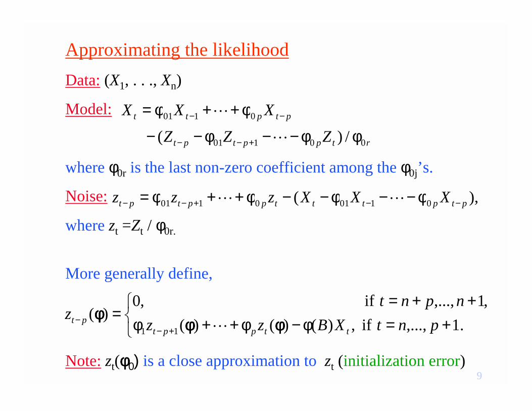
Approximating the likelihoodData: (X1, . . ., Xn)

Model:

where φ0r is the last non-zero coefficient among the φ0j’s.

Noise:

where zt =Zt / φ0r.

More generally define,

Note: zt(φφφφ0) is a close approximation to zt (initialization error)

rtpptpt

ptptt

ZZZXXX

00101

0101

/)( φφ−−φ−−

φ++φ=

+−−

−−

�

�

),( 01010101 ptptttpptpt XXXzzz −−+−− φ−−φ−−φ++φ= ��

+=φ−φ++φ++=

=+−

− .1,..., if ,)()()(,1,..., if ,0

)(11 pntXBzz

npntz

ttpptpt φφφφφφφφφφφφ

m

10

Assume that Zt has density function fσ and consider the vector

Joint density of z:

and hence the joint density of the data can be approximated by

where q=max{0 ≤ j ≤ p: φj ≠ 0}.

)')(),...,(),...,(,)(),...,(,,...,( 110101OOOO NOOOO MLOOOOO NOOOOO ML

φφφφφφφφφφφφφφφφφφφφ npnpp zzzzzXX +−−−=z

independent pieces

)),(),...,(( ||))((

))(),...,(,,...,()(

121

01011

φφφφφφφφφφφφ

φφφφφφφφ

npn

pn

tqtq

pp

zzhzf

zzXXhh

+−

−

=σ

−−

φφ•

=

∏

z

φφ= ∏

−

=σ

pn

tqtq zfh

1

||))(()( φφφφx

11

Log-likelihood:

where fσ(z)= σ−1 f(z/σ).

Least absolute deviations: choose Laplace density

and log-likelihood becomes

Concentrated Laplacian likelihood

Maximizing l(φφφφ) is equivalent to minimizing the absolute deviations

))((ln|)|/ln()(),(1

1 φφφφφφφφ ∑−

=

− φσ+φσ−−=σpn

ttqq zfpnL

|)|2exp(2

1)( zzf −=

||/ ,/|)(|2ln)(constant1

q

pn

ttzpn φσ=κκ−κ−− ∑

−

=

φφφφ

|)(|ln)(constant)(1

φφφφφφφφ ∑−

=

−−=pn

ttzpnl

.|)(|)(1

n φφφφφφφφ ∑−

=

=pn

ttzm

12

Assumptions for MLE

� Assume {Zt} iid fσ(z)=σ−1f(σ−1z) with

• σ a scale parameter

• mean 0, variance σ2

• further smoothness assumptions (integrability,symmetry, etc.) on f

• Fisher information:

Results

� Let γ(h) = ACVF of AR model with AR poly φ0(.) and

�

dzzfzfI )(/))('(~ 22∫

−σ=

p1kj,k)]-j([ =γ=Γp

))1~(2

1,0() ˆ( 1220MLE

−Γσ−σ

→− p

D

INn φφφφφφφφ

13

Further comments on MLE

Let α=(φ1, . . . , φp, σ /|φp|, β1, . . . , βq), where β1, . . . , βq are theparameters of pdf f.

Set

�

�

�

� (Fisher Information)

{ }

dzzfzfzf

dzzfzfzfz

dzzfzfz

dzzfzf

T

f

p

p

0000

0000

0000

0000

00000000

0000

0000

0000

0000

00000000

00000000

ββββββββ

ββββββββ

ββββββββ

ββββββββ

ββββββββ

ββββββββ

ββββββββ

∂∂

∂∂=

∂∂α−=

−α=

σ=

∫

∫

∫

∫

−+

−+

−

);();();(

1)(I

);();();('L

1);(/));('(K

);(/));('(I

11,0

2221,0

220

14

Under smoothness conditions on f wrt β1, . . . , βq we have

where

Note: is asymptotically independent of and

),,0() ˆ( 10MLE

−∑→− Nn

Dαααααααα

−−−−−−

Γσ−σ

=∑−−−−−

−−−−−

−

−

11111

11111

1220

1

)'ˆ(ˆ)'ˆ()'ˆ('ˆ)'ˆ(

)1ˆ(21

LKLIKLLKLILKLILKLILK

I

ff

ff

p

00

00

ˆMLEφφφφ ˆ MLE1,p+α ˆ

MLEββββ

15

Asymptotic Covariance Matrix• For LS estimators of AR(p):

• For LAD estimators of AR(p):

• For LAD estimators of AP(p):

• For MLE estimators of AP(p):

),0() ˆ( 120LS

−Γσ→− p

DNn φφφφφφφφ

))0(4

1,0() ˆ( 12220LAD

−Γσσ

→− p

D

fNn φφφφφφφφ

))1ˆ(2

1,0() ˆ( 1220MLE

−Γσ−σ

→− p

D

INn φφφφφφφφ

)|)|)0(2(2

|)(|Var,0() ˆ( 122

12

10LAD

−

σ

Γσ−σ

→− p

D

ZEfZNn φφφφφφφφ

16

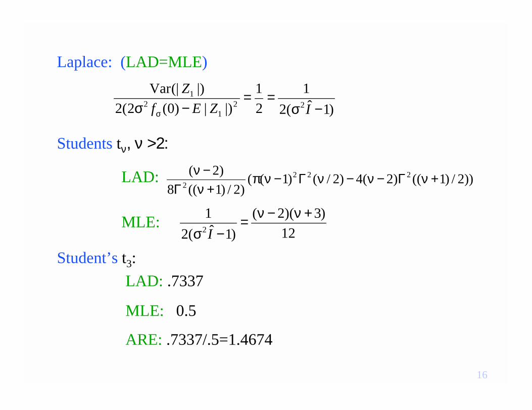
Laplace: (LAD=MLE)

Students tν, ν >2:

LAD:

MLE:

Student’s t3: LAD: .7337

MLE: 0.5

ARE: .7337/.5=1.4674

)1ˆ(21

21

|)|)0(2(2|)(|Var

221

21

−σ==

−σ σ IZEfZ

))2/)1(()2(4)2/()1(()2/)1((8

)2( 2222 +νΓ−ν−νΓ−νπ

+νΓ−ν

12)3)(2(

)1ˆ(21

2

+ν−ν=−σ I

17

R-Estimation:

Minimize the objective function

where {z(t)(φφφφ)} are the ordered {zt(φφφφ)}, and the weight function ϕ satisfies:

• ϕ is differentiable and nondecreasing on (0,1)

• ϕ´ is uniformly continuous

• ϕ(x) = −ϕ(1−x)Remarks:

•

• For LAD, take

)(1

( )(1t

φφφφφ)φ)φ)φ) t

pn

zpntS ∑

−

=

+−ϕ=

)(1

((1t

φφφφφ)φ)φ)φ)φ)φ)φ)φ) t

pnt zpn

RS ∑−

=

+−ϕ=

1.x1/2 1,

1/2,x0 1,-)(

<<<<

=ϕ x

18

Assumptions for R-estimation

� Assume {Zt} iid with density function f (distr F)

• mean 0, variance σ2

� Assume weight function ϕ is nondecreasing and continuously differentiable with ϕ(x) = −ϕ(1−x)

Results

� Set

� If then

∫∫∫ ϕ=ϕ=ϕ= −−1

0

11

0

11

0

2 )('))((L~ ,)()(K~ ,)(J~ dsssFfdsssFdss

))~~(2

~~,0() ˆ( 12

22

22

0R−Γσ

−σ−σ→− p

D

KLKJNn φφφφφφφφ

,~~2 KL >σ

19

Further comments on R-estimation

�ϕ(x) = x−1/2 is called the Wilcoxon weight function

� By formally choosing we obtain

That is R = LAD, asymptotically.

� The R-estimation objective function is smoother than the LAD-objective function and hence easier to minimize.

1.x1/2 1,

1/2,x0 1,-)(

<<<<

=ϕ x

.|)|)0(2(2

|)(|Var)~~(2

~~12

21

2112

22

22−

σ

− Γσ−σ

=Γσ−σ−σ

pp ZEfZ

KLKJ

20phi

-0.5 0.0 0.5

22.0

22.5

23.0

23.5

24.0

24.5

Objective Functions

R-estimation

LAD

21

Summary of asymptotics

� Maximum likelihood:

� R-estimation

�Least absolute deviations:

))1~(2

1,0() ˆ( 1220MLE

−Γσ−σ

→− p

D

INn φφφφφφφφ

)|)|)0(2(2

|)(|Var,0() ˆ( 122

12

10LAD

−

σ

Γσ−σ

→− p

D

ZEfZNn φφφφφφφφ

))~~(2

~~,0() ˆ( 12

22

22

0R−Γσ

−σ−σ→− p

D

KLKJNn φφφφφφφφ

22

Laplace: (LAD=MLE)

R: (using ϕ(x) = x−1/2, Wilcoxon)

LAD=MLE: 1/2

Students tν:

65

)~~(2

~~22

22

=−σ−σ

KLKJ

ν LAD R MLE LAD/R MLE/R3 .733 .520 .500 1.411 .9626 6.22 3.01 3.00 2.068 .9979 16.8 7.15 7.00 2.354 .98012 32.6 13.0 12.5 2.510 .96415 53.4 20.5 19.5 2.607 .95220 99.6 36.8 34.5 2.707 .93730 234 83.6 77.0 2.810 .921

23

Central Limit Theorem (R-estimation)

• Think of u = n1/2(φφφφ−−−−φφφφ0000) as an element of RRp

• Define

where Rt(φφφφ) is the rank of zt(φφφφ) among z1(φφφφ), . . ., zn-p(φφφφ).

• Then Sn(u) → S(u) in distribution on C(RRp), where

• Hence,

,)()1) ((- )()

1) (()(

10

0

1

1/2-0

-1/20 ∑∑

−

=

−

=

+−ϕ

+

+−+ϕ=

pn

tt

tpn

tt

tn z

pnRnz

pnnRS φφφφφφφφφφφφφφφφ uuu

),||)~~(2 ,(~ ,'')~~(||)( 220

222210 prpr KJNKLS Γσφ−σ+Γσ−σφ= −−−− 0NNuuuu

)||)~~(2

~~,(~

)~~(2||

)(minarg)ˆ()(minarg

122

022

2212

20

02/1

−− Γσφ−σ

−σΓσ−σ

φ−=

→−=

pr

pr

D

Rn

KLKJN

KL

SnS

0N

uu φφφφφφφφ

24

Main ideas (R-estimation)• Define

where Fz is the df of zt.

• Using a Taylor series, we have

• Also,

• Hence

,)())((- )())(()(~1

01

1/2-0 ∑∑

−

=

−

=

ϕ+ϕ=pn

tttz

pn

tttzn zzFnzzFS φφφφφφφφ uu

uuNu

uuuu

prD

pn

t

ttz

pn

t

ttzn

K

zzFnzzFnS

Γσφ−→

∂∂∂ϕ+

∂∂ϕ

−−

−

=

−−

=∑∑

210

1

02

1-1

1

01/2-

||~''

')())(('2 )())(('~)(~

φφφφφφφφφφφφ

φφφφφφφφ

).1(||/~')(~)( 022

prpnn oLSS +φΓσσ=− − uuuu

).||)~~(2 ,(~ ,'')~~(||)( 220

222210 prprDn KJNKLS Γσφ−σ+Γσ−σφ→ −−−− 0NNuuuu

25

Order Selection:

Partial ACF From the previous result, if true model is of order r and fitted model is of order p > r, then

where is the pth element of .

Procedure:

1. Fit high order (P-th order), obtain residuals and estimate scalar,

by empirical moments of residuals and density estimates.

)|)|)0(2(2

|)(|Var,0(ˆ2

12

1,

2/1

ZEfZNn LADp −σ

→φσ

LADp,φ LADφφφφ

21

212

|)|)0(2(2|)(|Var

ZEfZ−σ

=θσ

26

2. Fit AP models of order p=1,2, . . . , P via LAD and obtain p-th

coefficient for each.

3. Choose model order r as the smallest order beyond which the

estimated coefficients are statistically insignificant.

Note: Can replace with if using MLE. In this case

for p > r

pp ,φ

pp ,φ MLE,ˆ

pφ

).)1ˆ(2

1,0(ˆ2,

2/1

−σ→φ

INn MLEp

27

AIC: 2p or not 2p?

• An approximately unbiased estimate of the Kullback-Leiber index

of fitted to true model:

• Penalty term for Laplace case:

• Penalty term can be estimated from the data.

pZEf

ZEfZLpAIC X

−σ

−σ+κ−= σ

σ

1||)0(2

|)|)0(2(|)(|Var)ˆ,ˆ(2:)(

1

2

21

21φφφφ

ppZEf

ZEfZ =

−σ

−σσ

σ

1||)0(2

|)|)0(2(|)(|Var

1

2

21

21

28

Sample realization of all-pass of order 2

t

X(t)

0 100 200 300 400 500

-40

-20

020

(a) Data From Allpass Model

Lag

AC

F

0 10 20 30 40

0.0

0.2

0.4

0.6

0.8

1.0

(b) ACF of Allpass Data

Lag

AC

F

0 10 20 30 40

0.0

0.2

0.4

0.6

0.8

1.0

(c) ACF of Squares

Lag

AC

F

0 10 20 30 40

0.0

0.2

0.4

0.6

0.8

1.0

(d) ACF of Absolute Values

29

Simulation results:

• 1000 replicates of all-pass models

• model order parameter value 1 φ1 =.52 φ1=.3, φ2=.4

• noise distribution is t with 3 d.f.

• sample sizes n=500, 5000

• estimation method is LAD

30

To guard against being trapped in local minima, we adopted the following strategy.

• 250 random starting values were chosen at random. For model of order p, k-th starting value was computed recursively as follows:

1. Draw iid uniform (-1,1).2. For j=2, …, p, compute

• Select top 10 based on minimum function evaluation.

• Run Hooke and Jeeves with each of the 10 starting values and choose best optimized value.

)()(22

)(11 ,...,, k

ppkk φφφ

φ

φφ−

φ

φ=

φ

φ

−

−−

−−

−

−)(

1,1

)(1,1

)(

)(1,1

)(1,1

)(1,

)(1

kj

kjj

kjj

kjj

kj

kjj

kj

���

31

Asymptotic EmpiricalN mean std dev mean std dev %coverage rel eff*500 φ1=.5 .0332 .4979 .0397 94.2 11.85000 φ1=.5 .0105 .4998 .0109 95.4 9.3

Asymptotic EmpiricalN mean std dev mean std dev %coverage500 φ1=.3 .0351 .2990 .0456 92.5

φ2=.4 .0351 .3965 .0447 92.15000 φ1=.3 .0111 .3003 .0118 95.5

φ2=.4 .0111 .3990 .0117 94.7

*Efficiency relative to maximum absolute residual kurtosis:2

12

1t

4

2/12

))()((1 , 3)(1 φφφφφφφφφφφφ zzpn

vvz

pn t

pn

t

pnt −

−=−

− ∑∑−

=

−

=

32

Asymptotic EmpiricalN mean std dev mean std dev %coverage 500 φ1=.5 .0274 .4971 .0315 93.0

ν=3.0 .4480 3.112 .5008 95.8 5000 φ1=.5 .0087 .4997 .0091 93.4

ν=3.0 .1417 3.008 .1533 94.0

Asymptotic EmpiricalN mean std dev mean std dev %coverage500 φ1=.3 .0290 .2993 .0345 90.6

φ2=.4 .0290 .3964 .0350 90.1ν=3.0 .4480 3.079 .4722 94.8

5000 φ1=.3 .0092 .2999 .0095 94.0φ2=.4 .0092 .3999 .0094 94.6ν=3.0 .1417 3.008 .1458 95.2

MLE Simulations Results using t-distr(3.0)

33

Empirical Empirical LADN mean std dev mean std dev500 φ1=.5 .4978 .0315 .4979 .03975000 φ1=.5 .4997 .0094 .4998 .0109500 φ1=.3 .2988 .0374 .2990 .0456

φ2=.4 .3957 .0360 .3965 .04475000 φ1=.3 .3007 .0101 .3003 .0118

φ2=.4 .3993 .0104 .3990 .0117

R-Estimator: Minimize the objective fcn

where {z(t)(φφφφ)} are the ordered {zt(φφφφ)}.

)(21

1( )(

1tφφφφφ)φ)φ)φ) t

pn

zpntS ∑

−

=

−

+−=

34

Noninvertible MA models with heavy tailed noise

Xt = Zt + θ1 Zt-1 + + θq Zt-q ,

a. {Zt} ~ IID(α) with Pareto tails

b. θ(z) = 1 + θ1 z + + θq zq

No zeros inside the unit circle invertibleSome zero(s) inside the unit circle noninvertible

. . .

. . .

⇒

⇒

35

Realizations of an invertible and noninvertible MA(2) processesModel: Xt = θ∗ (B) Zt , {Zt} ~ IID(α = 1), whereθi(B) = (1 +1/2B)(1 + 1/3B) and θni(B) = (1 + 2B)(1 + 3B)

0 10 20 30 40

-40

-20

020

0 10 20 30 40

-300

-100

010

0

Lag

0 2 4 6 8 10

-0.2

0.2

0.6

1.0

ACF

Lag

0 2 4 6 8 10

-0.2

0.2

0.6

1.0

ACF

36

Application of all-pass to noninvertible MA model fitting

Suppose {Xt} follows the noninvertible MA model

Xt= θi(B) θni(B) Zt , {Zt} ~ IID.

Step 1: Let {Ut} be the residuals obtained by fitting a purely invertible MA model, i.e.,

So

Step 2: Fit a purely causal AP model to {Ut}

Z(B)~(B)U

). of version invertible theis ~( ,(B)U~(B)

(B)UˆX

tni

nit

ninitnii

tt

θθ≈

θθθθ≈

θ=

.(B)Z(B)U~tnitni θ=θ

37

t

X(t)

0 200 400 600

2*10

56*

105

106

Volumes of Microsoft (MSFT) stock traded over 755 transaction days (6/3/96 to 5/28/99)

38

Analysis of MSFT:

Step 1: Log(volume) follows MA(4).

Xt =(1+.513B+.277B2+.270B3+.202B4) Ut (invertible MA(4))

Step 2: All-pass model of order 4 fitted to {Ut} using MLE (t-dist):

(Model using R-estimation is nearly the same.)

Conclude that {Xt} follows a noninvertible MA(4) which after refitting has the form:

Xt =(1+1.34B+1.374B2+2.54B3+4.96B4) Zt , {Zt}~IID t(6.3)

6.26)ˆ( .)ZB960.43.116B1.135BB649.1(

)U02B2..131BB229..628B1(

t432

t432

=ν−++−=

−+−+−

39

Lag

ACF

0 10 20 30 40

0.0

0.4

0.8

(a) ACF of Squares of Ut

Lag

ACF

0 10 20 30 40

0.0

0.4

0.8

(b) ACF of Absolute Values of Ut

Lag

ACF

0 10 20 30 40

0.0

0.4

0.8

(c) ACF of Squares of Zt

Lag

ACF

0 10 20 30 40

0.0

0.4

0.8

(d) ACF of Absolute Values of Zt

40

Summary: Microsoft Trading Volume� Two-step fit of noninvertible MA(4):

• invertible MA(4): residuals not iid• causal AP(4); residuals iid

� Direct fit of purely noninvertible MA(4):(1+1.34B+1.374B2+2.54B3+4.96B4)

� For MCHP, invertible MA(4) fits.

41

Summary� All-pass models and their properties

• linear time series with “nonlinear” behavior� Estimation

• likelihood approximation• MLE, LAD, R-estimation• order selection

� Emprirical results• simulation study

�Noninvertible moving average processes• two-step estimation procedure using all-pass• noninvertible MA(4) for Microsoft trading volume

42

Further Work� Least absolute deviations

• further simulations• order selection• heavy-tailed case• other smooth objective functions (e.g., min dispersion)

� Maximum likelihood• Gaussian mixtures• simulation studies• applications

� Noninvertible moving average modeling• initial estimates from two-step all-pass procedure• adaptive procedures