Joint High Dynamic Range Imaging and Color Demosaicing

Johannes Herwig and Josef Pauli

University of Duisburg-Essen, Bismarckstr. 90, 47057 Duisburg, Germany

∗

ABSTRACT

A non-parametric high dynamic range (HDR) fusion approach is proposed that works on raw images of single-sensor color imaging devices which incorporate the Bayer pattern. Thereby the non-linear opto-electronic con-version function (OECF) is recovered before color demosaicing, so that interpolation artifacts do not affect thephotometric calibration. Graph-based segmentation greedily clusters the exposure set into regions of roughlyconstant radiance in order to regularize the OECF estimation. The segmentation works on Gaussian-blurredsensor images, whereby the artificial gray value edges caused by the Bayer pattern are smoothed away. Withthe OECF known the 32-bit HDR radiance map is reconstructed by weighted summation from the differentlyexposed raw sensor images. Because the radiance map contains lower sensor noise than the individual images, itis finally demosaiced by weighted bilinear interpolation which prevents the interpolation across edges. Here, theprevious segmentation results from the photometric calibration are utilized. After demosaicing, tone mapping isapplied, whereby remaining interpolation artifacts are further damped due to the coarser tonal quantization ofthe resulting image.

Keywords: Photometric Calibration, Image Fusion, Demosaicing, Image Acquisition

1. INTRODUCTION

Normally demosaicing1 is among the first processing steps in color image processing. In this paper a workflowof color segmentation and high dynamic range (HDR) rendering is proposed that places demosaicing at the endof the processing chain. The paper2 does something similar using a model of retinal processing. The paper3

computes the HDR image from RAW data of linear sensors (we are additionally calibrating the non-linearresponse curve) and lies its focus on better color reproduction. The following is essentially a fusion of our colorsegmentation approach presented in4 and the HDR calibration presented in5 which is itself an extension of6

using the model of the law of film from.7

1.1 Outline of the Approach

A non-parametric HDR fusion approach is proposed that works on raw images of single-sensor color imaging de-vices which incorporate the Bayer pattern. Thereby the non-linear opto-electronic conversion function (OECF)8

is recovered before color demosaicing, so that interpolation artifacts do not affect the photometric calibration.Next, the 32-bit HDR radiance map is reconstructed by weighted summation from the differently exposed rawsensor images. Because the radiance map contains lower sensor noise than the individual images, it is finally de-mosaiced by weighted bilinear interpolation which prevents the interpolation across edges. Then, tone mappingis applied, whereby remaining demosaicing artifacts are further damped due to the coarser tonal quantization ofthe resulting image.

∗ Copyright 2011 Society of Photo-Optical Instrumentation Engineers. One print or electronic copy may be made forpersonal use only. Systematic reproduction and distribution, duplication of any material in this paper for a fee or forcommercial purposes, or modification of the content of the paper are prohibited.

Johannes Herwig and Josef Pauli, ”Joint high dynamic range imaging and color demosaicing”, Image and Signal Process-ing for Remote Sensing XVII, Lorenzo Bruzzone, Volume 8180, Paper 8180-56, 2011, http://dx.doi.org/10.1117/12.898363

1.2 Photometric Calibration

Graph-based segmentation9 greedily clusters the exposure set into regions of roughly constant radiance, wherebyfirstly for each spatial location pixels with high local contrast, that belong to properly exposed regions, arechosen from the time domain, but secondly the remaining pixels should have small variations in order to belongto the same region5 (figure 8). The segmentation works on Gaussian-blurred sensor images, whereby the artificialgray value edges caused by the Bayer pattern are smoothed away.4 The non-linear OECF resembles the law offilm7 and is parametrized by its derivative. For every gray value the slope is robustly estimated by tracking thepreviously segmented regions throughout the exposure stack and relating them between successive exposures.5

A variation of the Debevec+Malik algorithm6 recovers the OECF per RGB plane from its first derivative.5

2. DEMOSAICING APPROACH

The raw image that is directly recorded by the sensor of an RGB camera is called the Bayer image, because itssingle-channel pixels are biased by the optical filter pattern of the Bayer mosaic. To obtain a full vector-valuedcolor image the two missing color components need to be interpolated from the local neighborhood of each pixel.This is known as demosaicing. The usual digital image processing pipeline starts with the demosaiced colorimage, because demosaicing is often internal to the camera driver and because the single-channel Bayer image isnot a straightforward representation for multi-channel color data.

In this paper it is proposed to perform mid-level image processing like color segmentation directly onto theraw Bayer image without previous demosaicing. The segmentation results are then used to parameterize low-level tasks like demosaicing and the creation of high dynamic range images (which both relate to the topic ofimage acquisition) with scene-dependent higher level information in order to achieve better results having lessinterpolation artifacts.

2.1 Gaussian Smoothing of Bayer Images

The Bayer representation of a color image has the advantage of being lightweight, because only real measurementdata is stored. Another advantage is being single-channel like a gray value image. Full color measurements on theother hand are vector-valued and feature at least three channels if we speak of ordinary RGB images. This triplesstorage costs but also processing times increase, because image processing algorithms are usually modeled witha single-channel representation of the scene or problem in mind where only spatial features of the distribution ofpixel measurements are concerned. Only as a subsequent processing step the correlation of spatial patterns inmultiple channels is exploited, or their presence and absence in specific channels leads to significant conclusionsabout the local spectral characteristics. Therefore the handling of vector-valued images is difficult, because eitherthe different channels need to be projected into some continuous single-channel luminance representation beforespatial processing or otherwise every channel needs to be separately processed with the same algorithm and latera fusion of the results may be needed. Both approaches to vector-image processing pose the problem of sensiblecolor metrics in order to extract (un)correlated spatial properties from the inter- and intra plane variations ofvector-valued data. Additionally, one has to cope with interpolation artifacts from the demosaicing algorithm.

Therefore it may be reasonable to apply color image processing on the Bayer image directly without previousdemosaicing. However, the Bayer representation has one great disadvantage which prevents one to do so easily.Because every neighbor of a given pixel is band-passed by a different optical color filter, artificial spatial gradientsare introduced w.r.t. every four-neighbor (and eight-neighbor for red and blue center pixels) which stem fromthe spectral properties of a given image patch. This plays against the aforementioned spatial model of imageprocessing algorithms which often analyze the local spatial change within an image plane to extract interestingfeatures within the signal. Because the Bayer pattern mixes spatial and spectral characteristics within theneighborhood of a pixel and because the sampling density of the different color channels varies (the greenchannel is sampled twice as dense as the red and blue channels), the common computation of local gradientsbecomes difficult to implement and is less precise since the step-size to the next pixel of the same color channeldepends on the channel itself, the location of the center pixel and the gradient direction. Therefore the error inthe gradient computation is not spatially isotropic within a single color channel and also the minimum systemimmanent error is smaller for green pixels than for red and blue pixels due to their different sampling density.

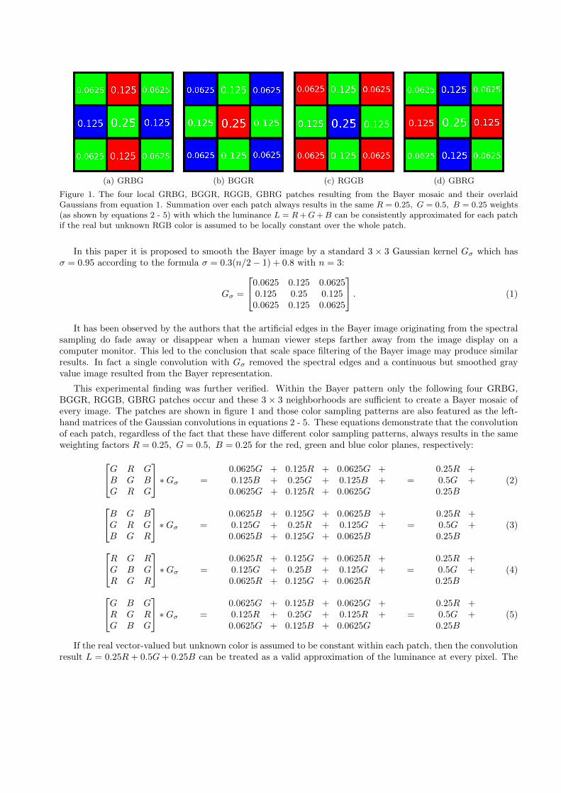
(a) GRBG (b) BGGR (c) RGGB (d) GBRG

Figure 1. The four local GRBG, BGGR, RGGB, GBRG patches resulting from the Bayer mosaic and their overlaidGaussians from equation 1. Summation over each patch always results in the same R = 0.25, G = 0.5, B = 0.25 weights(as shown by equations 2 - 5) with which the luminance L = R +G+B can be consistently approximated for each patchif the real but unknown RGB color is assumed to be locally constant over the whole patch.

In this paper it is proposed to smooth the Bayer image by a standard 3 × 3 Gaussian kernel Gσ which hasσ = 0.95 according to the formula σ = 0.3(n/2− 1) + 0.8 with n = 3:

Gσ =

0.0625 0.125 0.06250.125 0.25 0.1250.0625 0.125 0.0625

. (1)

It has been observed by the authors that the artificial edges in the Bayer image originating from the spectralsampling do fade away or disappear when a human viewer steps farther away from the image display on acomputer monitor. This led to the conclusion that scale space filtering of the Bayer image may produce similarresults. In fact a single convolution with Gσ removed the spectral edges and a continuous but smoothed grayvalue image resulted from the Bayer representation.

This experimental finding was further verified. Within the Bayer pattern only the following four GRBG,BGGR, RGGB, GBRG patches occur and these 3 × 3 neighborhoods are sufficient to create a Bayer mosaic ofevery image. The patches are shown in figure 1 and those color sampling patterns are also featured as the left-hand matrices of the Gaussian convolutions in equations 2 - 5. These equations demonstrate that the convolutionof each patch, regardless of the fact that these have different color sampling patterns, always results in the sameweighting factors R = 0.25, G = 0.5, B = 0.25 for the red, green and blue color planes, respectively:G R G

B G BG R G

∗Gσ =0.0625G + 0.125R + 0.0625G +0.125B + 0.25G + 0.125B +0.0625G + 0.125R + 0.0625G

=0.25R +0.5G +0.25B

(2)

B G BG R GB G R

∗Gσ =0.0625B + 0.125G + 0.0625B +0.125G + 0.25R + 0.125G +0.0625B + 0.125G + 0.0625B

=0.25R +0.5G +0.25B

(3)

R G RG B GR G R

∗Gσ =0.0625R + 0.125G + 0.0625R +0.125G + 0.25B + 0.125G +0.0625R + 0.125G + 0.0625R

=0.25R +0.5G +0.25B

(4)

G B GR G RG B G

∗Gσ =0.0625G + 0.125B + 0.0625G +0.125R + 0.25G + 0.125R +0.0625G + 0.125B + 0.0625G

=0.25R +0.5G +0.25B

(5)

If the real vector-valued but unknown color is assumed to be constant within each patch, then the convolutionresult L = 0.25R + 0.5G+ 0.25B can be treated as a valid approximation of the luminance at every pixel. The

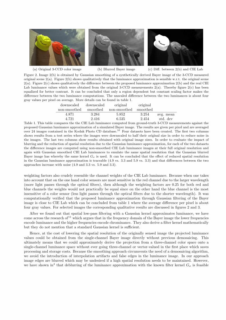
(a) Original 3-CCD color image (b) Blurred Bayer image (c) Diff. between 2(b) and CIE Lab

Figure 2. Image 2(b) is obtained by Gaussian smoothing of a synthetically derived Bayer image of the 3-CCD measuredoriginal scene 2(a). Figure 2(b) shows qualitatively that the luminance approximation is sensible w.r.t. the original scene2(a). Figure 2(c) shows qualitatively the difference between the proposed luminance approximation 2(b) and the real CIELab luminance values which were obtained from the original 3-CCD measurements 2(a). Thereby figure 2(c) has beenequalized for better contrast. It can be concluded that only a region dependent but constant scaling factor makes thedifference between the two luminance computations. The unscaled difference between the two luminances is about fourgray values per pixel on average. More details can be found in table 1.

downscaled downscaled original originalnon-smoothed smoothed non-smoothed smoothed

4.871 3.284 5.852 3.254 avg. mean4.721 2.416 6.535 2.454 std. dev

Table 1. This table compares the the CIE Lab luminance computed from ground-truth 3-CCD measurements against theproposed Gaussian luminance approximation of a simulated Bayer image. The results are given per pixel and are averagedover 24 images contained in the Kodak Photo CD database.10 Four datasets have been created. The first two columnsshows results from a test series where the images were downscaled to half their original size in order to reduce noise inthe images. The last two columns show results obtained with original image sizes. In order to evaluate the impact ofblurring and the reduction of spatial resolution due to the Gaussian luminance approximation, for each of the two datasetsthe difference images are computed using non-smoothed CIE Lab luminance images at their full original resolution andagain with Gaussian smoothed CIE Lab luminances to emulate the same spatial resolution that the Gaussian blurredBayer image has whereby the same kernel Gσ is used. It can be concluded that the effect of reduced spatial resolutionin the Gaussian luminance approximation is traceable (4.9 vs. 3.3 and 5.9 vs. 3.3) and that differences between the twoapproaches increase with noise (4.9 and 3.3 vs. 5.9 and 3.3).

weighting factors also crudely resemble the channel weights of the CIE Lab luminance. Because when one takesinto account that on the one hand color sensors are most sensitive in the red channel due to the larger wavelength(more light passes through the optical filters), then although the weighting factors are 0.25 for both red andblue channels the weights would not practically be equal since on the other hand the blue channel is the mostinsensitive of a color sensor (less light passes through the optical filters due to the shorter wavelength). It wascomputationally verified that the proposed luminance approximation through Gaussian filtering of the Bayerimage is close to CIE Lab which can be concluded from table 1 where the average difference per pixel is aboutfour gray values. For selected images the corresponding qualitative results are discussed in figures 2 and 3.

After we found out that spatial low-pass filtering with a Gaussian kernel approximates luminance, we havecome across the research of11 which argues that in the frequency domain of the Bayer image the lower frequenciesencode luminance and the higher frequencies encode chrominance. They also derive a filter kernel mathematicallybut they do not mention that a standard Gaussian kernel is sufficient.

Hence, at the cost of lowering the spatial resolution of the originally sensed image the projected luminancevalues could be obtained from the single-channel Bayer image directly without previous demosaicing. Thisultimately means that we could approximately derive the projection from a three-channel color space onto asingle-channel luminance space without ever going three-channel or vector-valued in the first place which savesprocessing and storage costs. Because the smoothing approach circumvents the need of a demosaicing algorithm,we avoid the introduction of interpolation artifacts and false edges in the luminance image. In our approachimage edges are blurred which may be undesired if a high spatial resolution needs to be maintained. However,we have shown in4 that deblurring of the luminance approximation with the known filter kernel Gσ is feasible

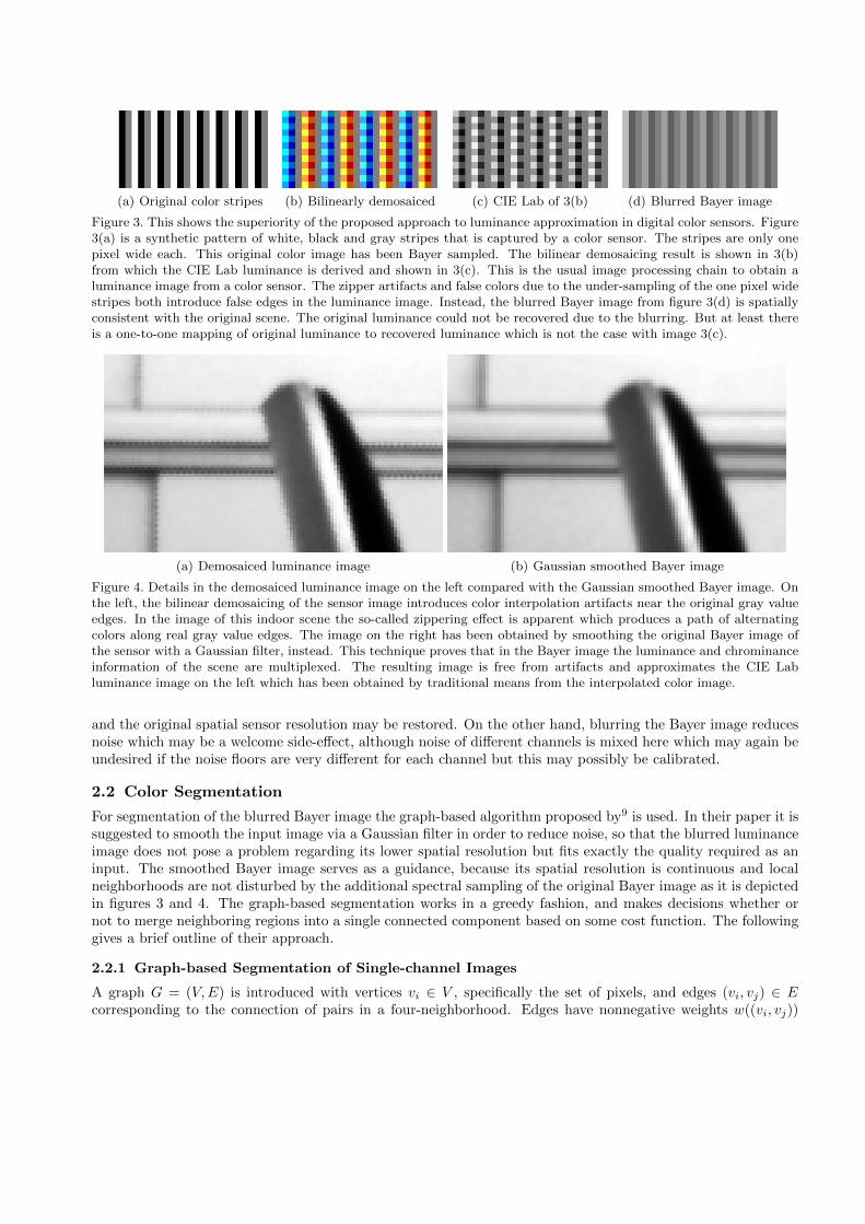
(a) Original color stripes (b) Bilinearly demosaiced (c) CIE Lab of 3(b) (d) Blurred Bayer image

Figure 3. This shows the superiority of the proposed approach to luminance approximation in digital color sensors. Figure3(a) is a synthetic pattern of white, black and gray stripes that is captured by a color sensor. The stripes are only onepixel wide each. This original color image has been Bayer sampled. The bilinear demosaicing result is shown in 3(b)from which the CIE Lab luminance is derived and shown in 3(c). This is the usual image processing chain to obtain aluminance image from a color sensor. The zipper artifacts and false colors due to the under-sampling of the one pixel widestripes both introduce false edges in the luminance image. Instead, the blurred Bayer image from figure 3(d) is spatiallyconsistent with the original scene. The original luminance could not be recovered due to the blurring. But at least thereis a one-to-one mapping of original luminance to recovered luminance which is not the case with image 3(c).

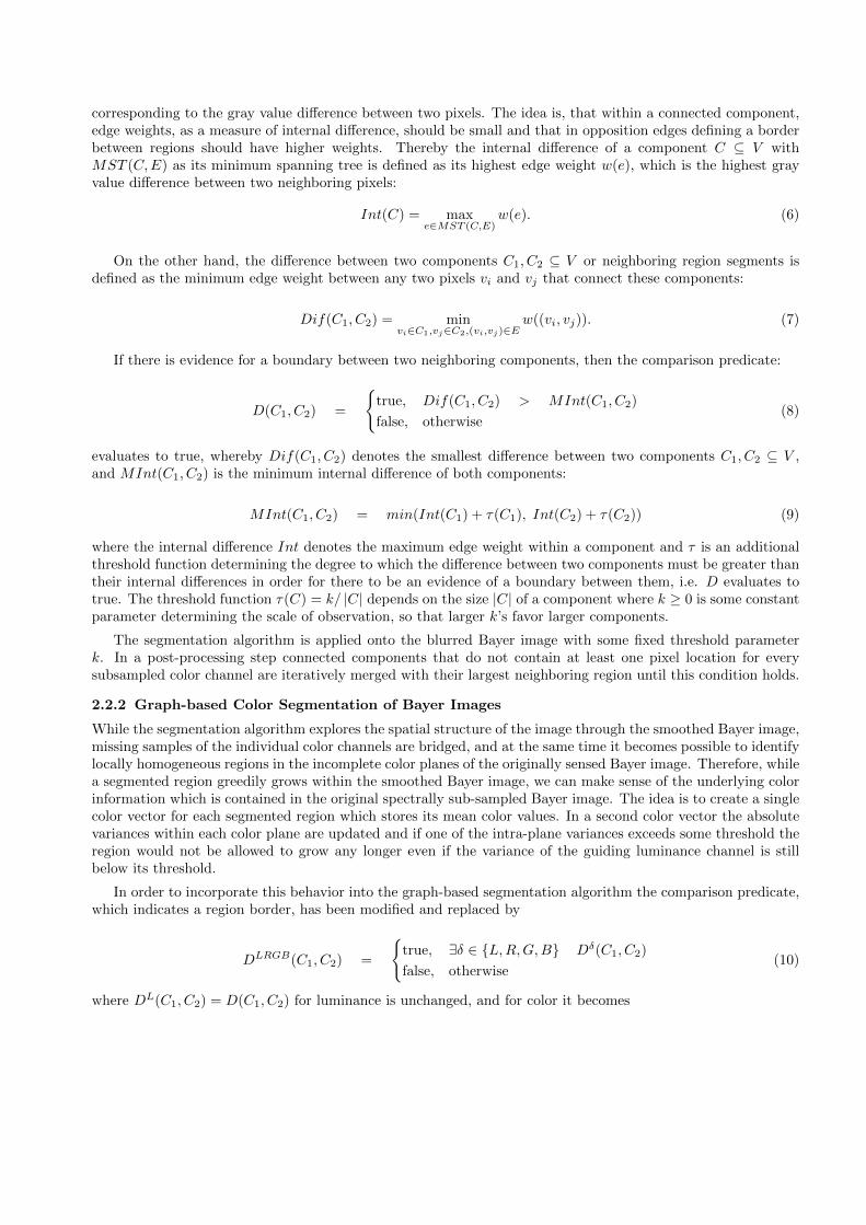
(a) Demosaiced luminance image (b) Gaussian smoothed Bayer image

Figure 4. Details in the demosaiced luminance image on the left compared with the Gaussian smoothed Bayer image. Onthe left, the bilinear demosaicing of the sensor image introduces color interpolation artifacts near the original gray valueedges. In the image of this indoor scene the so-called zippering effect is apparent which produces a path of alternatingcolors along real gray value edges. The image on the right has been obtained by smoothing the original Bayer image ofthe sensor with a Gaussian filter, instead. This technique proves that in the Bayer image the luminance and chrominanceinformation of the scene are multiplexed. The resulting image is free from artifacts and approximates the CIE Labluminance image on the left which has been obtained by traditional means from the interpolated color image.

and the original spatial sensor resolution may be restored. On the other hand, blurring the Bayer image reducesnoise which may be a welcome side-effect, although noise of different channels is mixed here which may again beundesired if the noise floors are very different for each channel but this may possibly be calibrated.

2.2 Color Segmentation

For segmentation of the blurred Bayer image the graph-based algorithm proposed by9 is used. In their paper it issuggested to smooth the input image via a Gaussian filter in order to reduce noise, so that the blurred luminanceimage does not pose a problem regarding its lower spatial resolution but fits exactly the quality required as aninput. The smoothed Bayer image serves as a guidance, because its spatial resolution is continuous and localneighborhoods are not disturbed by the additional spectral sampling of the original Bayer image as it is depictedin figures 3 and 4. The graph-based segmentation works in a greedy fashion, and makes decisions whether ornot to merge neighboring regions into a single connected component based on some cost function. The followinggives a brief outline of their approach.

2.2.1 Graph-based Segmentation of Single-channel Images

A graph G = (V,E) is introduced with vertices vi ∈ V , specifically the set of pixels, and edges (vi, vj) ∈ Ecorresponding to the connection of pairs in a four-neighborhood. Edges have nonnegative weights w((vi, vj))

corresponding to the gray value difference between two pixels. The idea is, that within a connected component,edge weights, as a measure of internal difference, should be small and that in opposition edges defining a borderbetween regions should have higher weights. Thereby the internal difference of a component C ⊆ V withMST (C,E) as its minimum spanning tree is defined as its highest edge weight w(e), which is the highest grayvalue difference between two neighboring pixels:

Int(C) = maxe∈MST (C,E)

w(e). (6)

On the other hand, the difference between two components C1, C2 ⊆ V or neighboring region segments isdefined as the minimum edge weight between any two pixels vi and vj that connect these components:

Dif(C1, C2) = minvi∈C1,vj∈C2,(vi,vj)∈E

w((vi, vj)). (7)

If there is evidence for a boundary between two neighboring components, then the comparison predicate:

D(C1, C2) =

{true, Dif(C1, C2) > MInt(C1, C2)

false, otherwise(8)

evaluates to true, whereby Dif(C1, C2) denotes the smallest difference between two components C1, C2 ⊆ V ,and MInt(C1, C2) is the minimum internal difference of both components:

MInt(C1, C2) = min(Int(C1) + τ(C1), Int(C2) + τ(C2)) (9)

where the internal difference Int denotes the maximum edge weight within a component and τ is an additionalthreshold function determining the degree to which the difference between two components must be greater thantheir internal differences in order for there to be an evidence of a boundary between them, i.e. D evaluates totrue. The threshold function τ(C) = k/ |C| depends on the size |C| of a component where k ≥ 0 is some constantparameter determining the scale of observation, so that larger k’s favor larger components.

The segmentation algorithm is applied onto the blurred Bayer image with some fixed threshold parameterk. In a post-processing step connected components that do not contain at least one pixel location for everysubsampled color channel are iteratively merged with their largest neighboring region until this condition holds.

2.2.2 Graph-based Color Segmentation of Bayer Images

While the segmentation algorithm explores the spatial structure of the image through the smoothed Bayer image,missing samples of the individual color channels are bridged, and at the same time it becomes possible to identifylocally homogeneous regions in the incomplete color planes of the originally sensed Bayer image. Therefore, whilea segmented region greedily grows within the smoothed Bayer image, we can make sense of the underlying colorinformation which is contained in the original spectrally sub-sampled Bayer image. The idea is to create a singlecolor vector for each segmented region which stores its mean color values. In a second color vector the absolutevariances within each color plane are updated and if one of the intra-plane variances exceeds some threshold theregion would not be allowed to grow any longer even if the variance of the guiding luminance channel is stillbelow its threshold.

In order to incorporate this behavior into the graph-based segmentation algorithm the comparison predicate,which indicates a region border, has been modified and replaced by

DLRGB(C1, C2) =

{true, ∃δ ∈ {L,R,G,B} Dδ(C1, C2)

false, otherwise(10)

where DL(C1, C2) = D(C1, C2) for luminance is unchanged, and for color it becomes

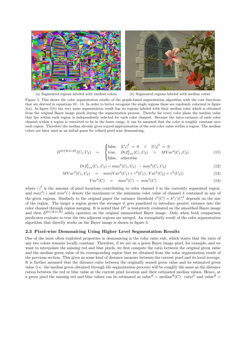
(a) Segmented regions labeled with random colors (b) Segmented regions labeled with median colors

Figure 5. This shows the color segmentation results of the graph-based segmentation algorithm with the cost functionsthat are derived in equations 10 - 14. In order to better recognize the single regions these are randomly colorized in figure5(a). In figure 5(b) the very same segmentation result has its regions labeled with their median color which is obtainedfrom the original Bayer image pixels during the segmentation process. Thereby for every color plane the median valuethat lies within each region is independently selected for each color channel. Because the intra-variance of each colorchannel within a region is restricted to be in the lower range, it can be assumed that the color is roughly constant overeach region. Therefore the median already gives a good approximation of the real color value within a region. The mediancolors are later used as an initial guess for refined pixel-wise demosaicing.

Dδ∈{R,G,B}(C1, C2) =

false, |C1|δ = 0 ∨ |C2|δ = 0

true, DifδV ar(C1, C2) > MV arδ(C1, C2)

false, otherwise

(11)

DifδV ar(C1, C2) = maxδ(C1, C2) − minδ(C1, C2) (12)

MV arδ(C1, C2) = min(V arδ(C1) + τ δ(C1), V arδ(C2) + τ δ(C2)) (13)

V arδ(C) = maxδ(C) − minδ(C) (14)

where |·|δ is the amount of pixel locations contributing to color channel δ in the currently segmented region,and maxδ(·) and minδ(·) denote the maximum or the minimum color value of channel δ contained in any of

the given regions. Similarly to the original paper the variance threshold τ δ(C) = kδ/ |C|δ depends on the sizeof the region. The larger a region grows the stronger it gets panelized to introduce greater variance into thecolor channel through region merging. It is noted that DL is tentatively evaluated on the smoothed Bayer imageand then Dδ∈{R,G,B} solely operates on the original unsmoothed Bayer image. Only when both comparisonpredicates evaluate to true the two adjacent regions are merged. An exemplarily result of the color segmentationalgorithm that directly works on the Bayer image is shown in figure 5.

2.3 Pixel-wise Demosaicing Using Higher Level Segmentation Results

One of the most often exploited properties in demosaicing is the color ratio rule, which states that the ratio ofany two colors remains locally constant. Therefore, if we are on a green Bayer image pixel, for example, and wewant to interpolate the missing red and blue pixels, we first compute the ratio between the original green valueand the median green value of its corresponding region that we obtained from the color segmentation result ofthe previous section. This gives us some kind of distance measure between the current pixel and its local average.It is further assumed that the distance ratio between the originally sensed green value and its estimated greenvalue (i.e. the median green obtained through the segmentation process) will be roughly the same as the distanceration between the red or blue value at the current pixel location and their estimated median values. Hence, ata green pixel the missing red and blue values can be estimated as valueR = medianR(C)· ratioG and valueB =

(a) Bayer image (b) Randomly colored segments (c) Median colored segments

(d) Refined pixel-wise interpolation (e) Bilinear demosaicing (f) Original image

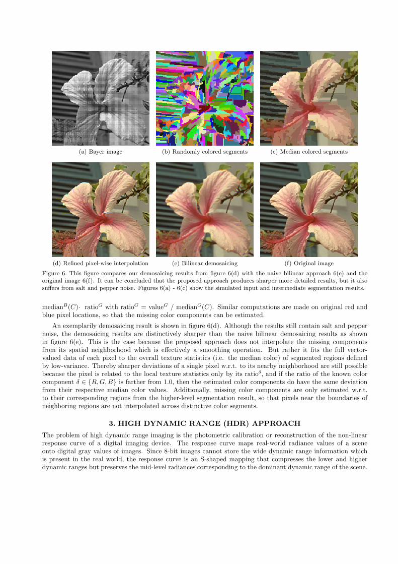
Figure 6. This figure compares our demosaicing results from figure 6(d) with the naive bilinear approach 6(e) and theoriginal image 6(f). It can be concluded that the proposed approach produces sharper more detailed results, but it alsosuffers from salt and pepper noise. Figures 6(a) - 6(c) show the simulated input and intermediate segmentation results.

medianB(C)· ratioG with ratioG = valueG / medianG(C). Similar computations are made on original red andblue pixel locations, so that the missing color components can be estimated.

An exemplarily demosaicing result is shown in figure 6(d). Although the results still contain salt and peppernoise, the demosaicing results are distinctively sharper than the naive bilinear demosaicing results as shownin figure 6(e). This is the case because the proposed approach does not interpolate the missing componentsfrom its spatial neighborhood which is effectively a smoothing operation. But rather it fits the full vector-valued data of each pixel to the overall texture statistics (i.e. the median color) of segmented regions definedby low-variance. Thereby sharper deviations of a single pixel w.r.t. to its nearby neighborhood are still possiblebecause the pixel is related to the local texture statistics only by its ratioδ, and if the ratio of the known colorcomponent δ ∈ {R,G,B} is farther from 1.0, then the estimated color components do have the same deviationfrom their respective median color values. Additionally, missing color components are only estimated w.r.t.to their corresponding regions from the higher-level segmentation result, so that pixels near the boundaries ofneighboring regions are not interpolated across distinctive color segments.

3. HIGH DYNAMIC RANGE (HDR) APPROACH

The problem of high dynamic range imaging is the photometric calibration or reconstruction of the non-linearresponse curve of a digital imaging device. The response curve maps real-world radiance values of a sceneonto digital gray values of images. Since 8-bit images cannot store the wide dynamic range information whichis present in the real world, the response curve is an S-shaped mapping that compresses the lower and higherdynamic ranges but preserves the mid-level radiances corresponding to the dominant dynamic range of the scene.

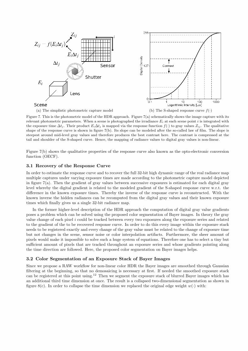
(a) The simplistic photometric capture model (b) The S-shaped response curve f(·)Figure 7. This is the photometric model of the HDR approach. Figure 7(a) schematically shows the image capture with itsrelevant photometric parameters. When a scene is photographed the irradiance Ei at each scene point i is integrated withthe exposure time ∆tj . Their product Ei∆tj is mapped via the response function f(·) to gray values Zij . The qualitativeshape of the response curve is shown in figure 7(b). Its slope can be modeled after the so-called law of film. The slope issteepest around mid-level gray values and therefore produces the best contrast here. The contrast is compressed at thetail and shoulder of the S-shaped curve. Hence, the mapping of radiance values to digital gray values is non-linear.

Figure 7(b) shows the qualitative properties of the response curve also known as the opto-electronic conversionfunction (OECF).

3.1 Recovery of the Response Curve

In order to estimate the response curve and to recover the full 32-bit high dynamic range of the real radiance mapmultiple captures under varying exposure times are made according to the photometric capture model depictedin figure 7(a). Then the gradient of gray values between successive exposures is estimated for each digital graylevel whereby the digital gradient is related to the modeled gradient of the S-shaped response curve w.r.t. thedifference in the known exposure times. Thereby the inverse of the response curve is reconstructed. With theknown inverse the hidden radiances can be recomputed from the digital gray values and their known exposuretimes which finally gives us a single 32-bit radiance map.

In the former higher-level description of the HDR approach the computation of digital gray value gradientsposes a problem which can be solved using the proposed color segmentation of Bayer images. In theory the grayvalue change of each pixel i could be tracked between every two exposures along the exposure series and relatedto the gradient of the to be recovered response curve. In order to do this every image within the exposure stackneeds to be registered exactly and every change of the gray value must be related to the change of exposure timebut not changes in the scene, sensor noise or color interpolation artifacts. Furthermore, the sheer amount ofpixels would make it impossible to solve such a huge system of equations. Therefore one has to select a tiny butsufficient amount of pixels that are tracked throughout an exposure series and whose gradients pointing alongthe time direction are followed. Here, the proposed color segmentation on Bayer images helps.

3.2 Color Segmentation of an Exposure Stack of Bayer Images

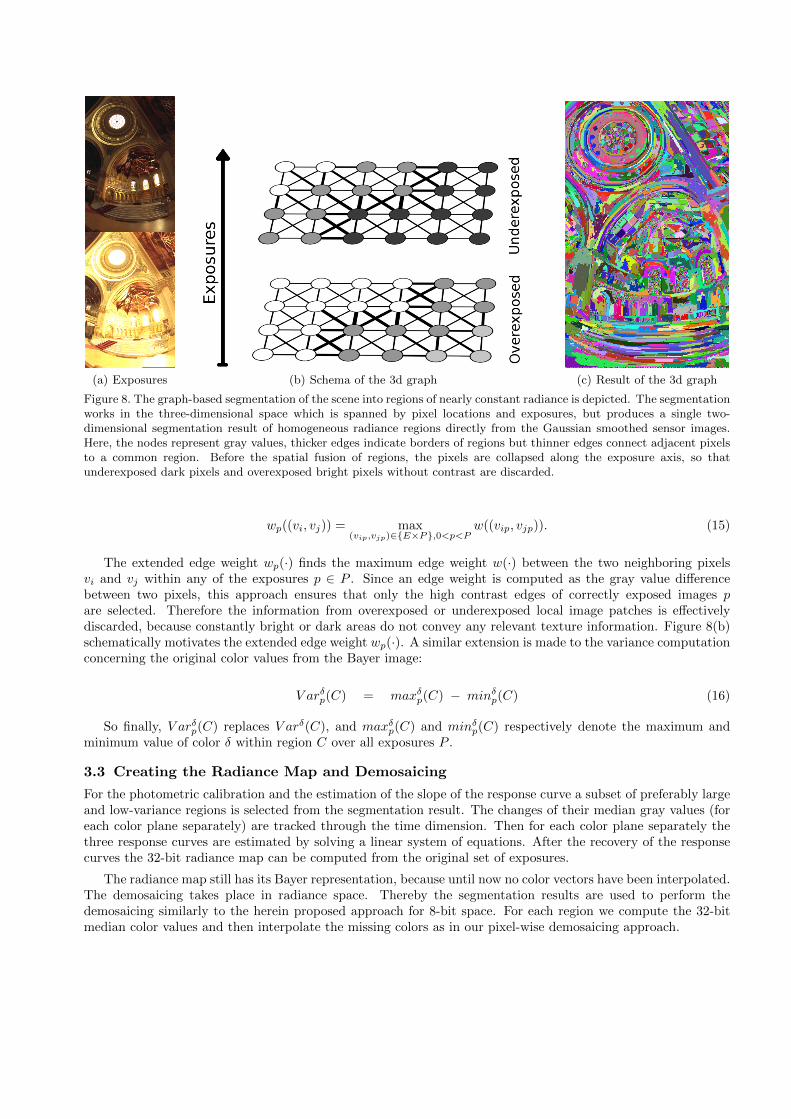
Since we propose a RAW workflow for non-linear color HDR the Bayer images are smoothed through Gaussianfiltering at the beginning, so that no demosaicing is necessary at first. If needed the smoothed exposure stackcan be registered at this point using.12 Then we segment the exposure stack of blurred Bayer images which hasan additional third time dimension at once. The result is a collapsed two-dimensional segmentation as shown infigure 8(c). In order to collapse the time dimension we replaced the original edge weight w(·) with:

(a) Exposures (b) Schema of the 3d graph (c) Result of the 3d graph

Figure 8. The graph-based segmentation of the scene into regions of nearly constant radiance is depicted. The segmentationworks in the three-dimensional space which is spanned by pixel locations and exposures, but produces a single two-dimensional segmentation result of homogeneous radiance regions directly from the Gaussian smoothed sensor images.Here, the nodes represent gray values, thicker edges indicate borders of regions but thinner edges connect adjacent pixelsto a common region. Before the spatial fusion of regions, the pixels are collapsed along the exposure axis, so thatunderexposed dark pixels and overexposed bright pixels without contrast are discarded.

wp((vi, vj)) = max(vip,vjp)∈{E×P},0<p<P

w((vip, vjp)). (15)

The extended edge weight wp(·) finds the maximum edge weight w(·) between the two neighboring pixelsvi and vj within any of the exposures p ∈ P . Since an edge weight is computed as the gray value differencebetween two pixels, this approach ensures that only the high contrast edges of correctly exposed images pare selected. Therefore the information from overexposed or underexposed local image patches is effectivelydiscarded, because constantly bright or dark areas do not convey any relevant texture information. Figure 8(b)schematically motivates the extended edge weight wp(·). A similar extension is made to the variance computationconcerning the original color values from the Bayer image:

V arδp(C) = maxδp(C) − minδp(C) (16)

So finally, V arδp(C) replaces V arδ(C), and maxδp(C) and minδp(C) respectively denote the maximum andminimum value of color δ within region C over all exposures P .

3.3 Creating the Radiance Map and Demosaicing

For the photometric calibration and the estimation of the slope of the response curve a subset of preferably largeand low-variance regions is selected from the segmentation result. The changes of their median gray values (foreach color plane separately) are tracked through the time dimension. Then for each color plane separately thethree response curves are estimated by solving a linear system of equations. After the recovery of the responsecurves the 32-bit radiance map can be computed from the original set of exposures.

The radiance map still has its Bayer representation, because until now no color vectors have been interpolated.The demosaicing takes place in radiance space. Thereby the segmentation results are used to perform thedemosaicing similarly to the herein proposed approach for 8-bit space. For each region we compute the 32-bitmedian color values and then interpolate the missing colors as in our pixel-wise demosaicing approach.

4. CONCLUSION

The photometric calibration of non-linear OECFs utilizes only raw sensor images. Gaussian smoothing of the sen-sor images approximates their luminance, so that these can be segmented before demosaicing. The unsupervisedsegmentation allows for automatic regularization of the OECF estimation. Demosaicing uses joint segmentationresults from multiple exposures at once in order to robustly prevent the interpolation across edges. The proposedluminance approximation of raw Bayer images through Gaussian smoothing allows one to design a single-channelimage processing chain for color images apart from the traditional vector-based approach.

REFERENCES

[1] Gunturk, B. K., Altunbasak, Y., and Mersereau, R. M., “Color plane interpolation using alternating pro-jections,” IEEE Transactions on Image Processing 11, 997–1013 (Sept. 2002).

[2] Tamburrino, D., Alleysson, D., Meylan, L., and Suesstrunk, S., “Digital camera workflow for high dynamicrange images using a model of retinal processing,” in [Proceedings of SPIE-The International Society forOptical Engineering ], DiCarlo, J. and Rodricks, B., eds., 6817 (2008).

[3] Joffre, G., Puech, W., Comby, F., and Joffre, J., “High dynamic range images from digital cameras rawdata,” in [ACM SIGGRAPH 2005 Posters ], (2005).

[4] Herwig, J. and Pauli, J., “Spatial Gaussian filtering of Bayer images with applications to color segmentation,”in [FarbBV2009 - 15. Workshop Farbbildverarbeitung ], 19–28 (2009).

[5] Herwig, J. and Pauli, J., “Recovery of the response curve of a digital imaging process by data-centricregularization,” in [VISAPP ], 1, 539–546 (2009).

[6] Debevec, P. E. and Malik, J., “Recovering high dynamic range radiance maps from photographs,” in [SIG-GRAPH ’97: Proceedings of the 24th annual conference on Computer graphics and interactive techniques ],369–378, ACM Press/Addison-Wesley Publishing Co., New York, NY, USA (1997).

[7] Mann, S. and Picard, R. W., “Being ’undigital’ with digital cameras: Extending Dynamic Range by Combin-ing Differently Exposed Pictures,” in [IS&T’s 48th annual conference Cambridge, Massachusetts ], 422–428,IS&T (May 1995).

[8] Sprawls, P., [Physical Principles of Medical Imaging ], Aspen Pub, 2nd ed. (May 1993).

[9] Felzenszwalb, P. F. and Huttenlocher, D. P., “Efficient Graph-Based Image Segmentation,” in [InternationalJournal of Computer Vision ], 59, 167–181, Springer (September 2004).

[10] Franzen, R., “Kodak Lossless True Color Image Suite,” (2004). Kodak PhotoCD PCD0992 image samplesin PNG file format.

[11] Alleysson, D., Susstrunk, S., and Herault, J., “Color Demosaicing by Estimating Luminance and OpponentChromatic Signals in the Fourier Domain,” in [Proc. IS&T/SID 10th Color Imaging Conference ], 10, 331–336 (2002).

[12] Ward, G., “Fast, robust image registration for compositing high dynamic range photographs from hand-heldexposures,” Journal of Graphics Tools 8(2), 17–30 (2003).

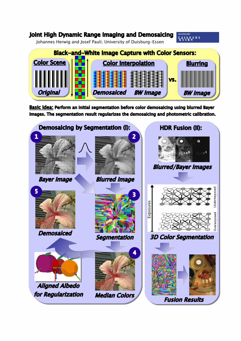
Joint High Dynamic Range Imaging and DemosaicingJohannes Herwig and Josef Pauli; University of Duisburg-Essen

Color SceneBlack-and-White Image Capture with Color Sensors:

Demosaiced BW Image

Blurring

BW Image

vs.

Original

Color Interpolation

Bayer Image Blurred Image

Segmentation

Median ColorsAligned Albedo

for Regularization

Demosaiced

1 2

3

4

5

Demosaicing by Segmentation (I):

Blurred/Bayer Images

3D Color Segmentation

Fusion Results

HDR Fusion (II):

Basic Idea: Perform an initial segmentation before color demosaicing using blurred BayerImages. The segmentation result regularizes the demosaicing and photometric calibration.