THE EFFECT OF SEGMENT CHARACTERISTICS

ON THE SEVERITY OF HEAD-ON CRASHES

ON TWO-LANE RURAL HIGHWAYS

John N. Ivan Per E. Garder Zuxuan Deng Chen Zhang

UNITED STATES DEPARTMENT OF TRANSPORTATION

REGION I UNIVERSITY TRANSPORTATION CENTER PROJECT UCNR15-5

FINAL REPORT January 5, 2006

Performed by

University of Connecticut Connecticut Transportation Institute

Storrs, CT 06269

And

University of Maine Department of Civil Engineering

Orono, ME 04469

- i -

TABLE OF CONTENTS

LIST OF FIGURES .................................................................................................................ii

LIST OF TABLES ................................................................................................................. iii

PART I. ANALYSIS IN CONNECTICUT ...........................................................................1

ABSTRACT...........................................................................................................................1

INTRODUCTION .................................................................................................................2

LITERATURE REVIEW ......................................................................................................5

STUDY DESIGN AND DATA COLLECTION...................................................................8

NEGATIVE BINOMIAL REGRESSION OF HEAD-ON CRASH INCIDENCE ............14

ORDERED PROBIT ANALYSIS OF HEAD-ON CRASH SEVERITY...........................19

SUMMARY AND CONCLUSIONS ..................................................................................31

REFERENCES ....................................................................................................................33

PART II. ANALYSIS IN MAINE ........................................................................................35

ABSTRACT.........................................................................................................................35

INTRODUCTION ...............................................................................................................36

DATA ..................................................................................................................................39

CRASH NUMBER RESULTS ............................................................................................40

SEVERITY CAUSATION RESULTS ................................................................................51

CONCLUSIONS AND DISCUSSION................................................................................56

REFERENCES ....................................................................................................................60

APPENDIX IIA: DATA......................................................................................................61

- ii -

LIST OF FIGURES Figure I-1. Effects of Change in X on Predicted Probabilities……………………………….20 Figure I-2. Frequency Pattern of RWIDTH………………………………………………….26 Figure I-3. Frequency Pattern of ACCESS…………………………………………………..26 Figure I-4. Crash severity by number of RETAIL driveways………………………………..30 Figure I-5. Crash severity by number of OFFICE driveways………………………………..30 Figure II-1. Crash and fatality proportions by crash type on rural non-Interstate highways...36 Figure II-2. Rescue personnel inspect pickup truck at scene of a fatal accident in Lebanon,

Maine…………………………………………………………………………………………37 Figure II-3. Likelihood of incapacitating or fatal injury……………………………………..51 Figure II-4. Likelihood of fatal injury in head-on collision………………………………….52 Figure II-5. 2+1-lane road……………………………………………………………………57 Figure II-6. 2+1-lane road with barrier………………………………………………………57

- iii -

LIST OF TABLES Table I-1. Collision Statistics by Number of Roadway Lanes………………………………...2 Table I-2. Motor Vehicle Collision Statistics by Number of Vehicles Involved…….…..........3 Table I-3. Motor Vehicle Collision Statistics by First Harmful Event…………...……….......3 Table I-4. Sample of Connecticut Dataset…………………………………............................12 Table I-5. Variable Definitions and Statistics………………………………………………..13 Table I-6. One-Variable GLIM Results……………………………………………………...15 Table I-7. Correlations (with Significance Level) Among Significant Variable.……………16 Table I-8. Final Models and AIC Test Results……………………………………………....16 Table I-9. Head-on Crash Severity as a Function of Crash Characteristics…………….........22 Table I-10. Head-on Crash Severity as a Function of Crash and Road Characteristics…...24 Table I-11. Correlation Analysis of Four Significant Variables……………………………..27 Table I-12. Definitions of Categorical Variables for WIDTH and ACCESS………………..27 Table I-13. Head-on Crash Severity as a Function of Categorical Crash and Road

Characteristics………………………………………………………………………………..27 Table I-14. Head-on crash severity as a function of crash and road characteristics with

different access type………………………………………………………………………….29 Table I-15. Crash severity distribution by number of retail and office driveways…………..30 Table II-1. Observed crash rates (crashes per mile per year) ranked from highest

down (to average)…………………….………………………………………………………41 Table II-2. Statistically proven unsafe roads and their (statistically not unlikely) minimum

crash rates (crashes per mile per year).………………………………………………………42 Table II-3. Statistically proven unsafe roads and their (statistically not unlikely) minimum

crash rates (crashes per hundred million vehicle-miles)……………………………………..42 Table II-4. Statistically proven safest routes and their (statistically not unlikely) maximum

crash rates (crashes per mile per year)……………………………………………………….43 Table II-5. Segments with multiple crashes in the three-year period………………………..43 Table II-6. One-mile segments with high crash rates and at least three crashes in the

three-year period…………………………………..…………………………………………44 Table II-7. Contributing factors/driver conditions/pre-crash actions for fatal crashes………48 Table II-8. Summary of primary contributing factors for fatal crashes……………………...48 Table II-9. Posted speed and severity of head-on crashes, Maine 2000-2002……………….51 Table II-10. Roadway class and severity of head-on crashes, Maine 2000-2002……………53 Table II-11. Two-lane, 45-mph roads and portion fatal or incapacitating injuries vs. shoulder

width and AADT……………………………………………………………………………..53 Table II-12. The influence of shoulder width for 2-lane, 50-mph roads……………………..54 Table II-13. Number of lanes and severity, excluding Interstates……………………………54 Table II-14. Number of lanes and severity for rural roads with speed limits 45 to 55 mph…55 Table II-15. Vehicle type and injury severity………………………………………………...55 Table II-16. Number of head-on crashes per route…………………………………………...61 Table II-17. Number of fatal crashes per route………………………………………………66

- 1 -

PART I. ANALYSIS IN CONNECTICUT ABSTRACT The National Center for Statistics and Analysis (NCSA) and the National Highway Traffic Safety Administration (NHTSA) suggest that head-on crashes are disproportionately represented in fatal crashes on two-lane highways, which constitute a substantial proportion of the highway network in the US. This study focuses on analyzing the correlation between head-on crash and potential causal factors, such as the geometric characteristics of the road segment, weather conditions, road surface conditions, and time of occurrence. Negative Binomial (NB) Generalized Linear Models (GLIM) were used to evaluate the effects of roadway geometric features on the incidence of head-on crashes on two-lane rural roads in Connecticut. Seven hundred and twenty highway segments, each with a uniform length of 1-km, were selected for analysis so that they contained no intersections with signal or stop control on the major road approaches. Head-on crash data were collected for these segments from the years 1996 through 2001. Variables found to significantly influence the incidence of head-on crashes were the speed limit, SACRH (sum of absolute change rate of horizontal curvature), MAXD (maximum degree of horizontal curve), and SACRV (sum of absolute change rate of vertical curvature). Three models were estimated with different combinations of the above four variables, and the performance of the models were tested using Akaike’s Information Criterion (AIC). The number of crashes was found to increase with each of these variables except for speed limit. Variables such as lane and shoulder width were not found to be significant for explaining the incidence of head-on crashes. Meanwhile, Ordered Probit models were estimated for datasets describing two-lane roads in Connecticut. It was found that a wet roadway surface and narrow road segments are significantly correlated with more severe head-on crashes. A high density of access points and a nighttime occurrence for the crash are significantly correlated with more severe cases. Pavement width is found to be the most consistent factor, possibly because a wider road offers more space to avoid a direct head-on impact, thus reducing the severity of the crash. Also, the vehicle braking performance is important, as suggested by the higher probability of severe head-on crashes on wet surfaces. The analysis results may be used by practitioners to understand the trade-off between geometric design decisions and head-on crash severity. Furthermore, identifying correlated factors will help to better explain the crash phenomenon and in turn can institute safer roadway design standards.

- 2 -

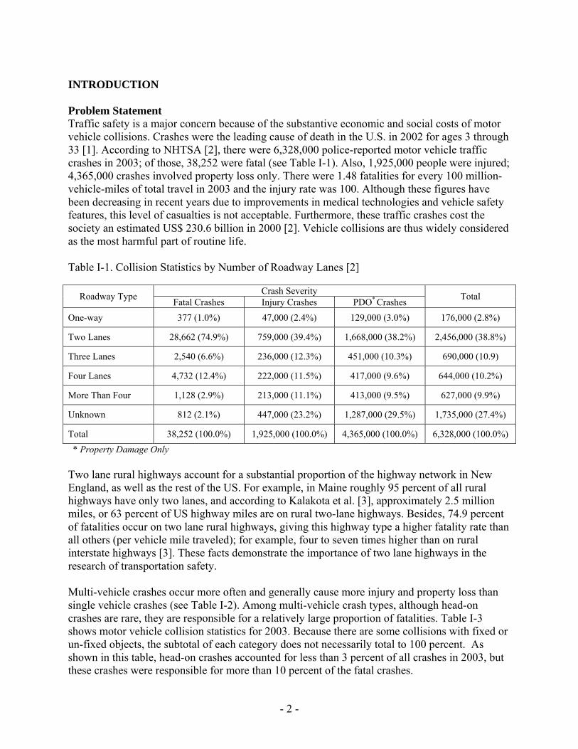
INTRODUCTION Problem Statement Traffic safety is a major concern because of the substantive economic and social costs of motor vehicle collisions. Crashes were the leading cause of death in the U.S. in 2002 for ages 3 through 33 [1]. According to NHTSA [2], there were 6,328,000 police-reported motor vehicle traffic crashes in 2003; of those, 38,252 were fatal (see Table I-1). Also, 1,925,000 people were injured; 4,365,000 crashes involved property loss only. There were 1.48 fatalities for every 100 million-vehicle-miles of total travel in 2003 and the injury rate was 100. Although these figures have been decreasing in recent years due to improvements in medical technologies and vehicle safety features, this level of casualties is not acceptable. Furthermore, these traffic crashes cost the society an estimated US$ 230.6 billion in 2000 [2]. Vehicle collisions are thus widely considered as the most harmful part of routine life. Table I-1. Collision Statistics by Number of Roadway Lanes [2]

Crash Severity Roadway Type Fatal Crashes Injury Crashes PDO* Crashes Total

One-way 377 (1.0%) 47,000 (2.4%) 129,000 (3.0%) 176,000 (2.8%)

Two Lanes 28,662 (74.9%) 759,000 (39.4%) 1,668,000 (38.2%) 2,456,000 (38.8%)

Three Lanes 2,540 (6.6%) 236,000 (12.3%) 451,000 (10.3%) 690,000 (10.9)

Four Lanes 4,732 (12.4%) 222,000 (11.5%) 417,000 (9.6%) 644,000 (10.2%)

More Than Four 1,128 (2.9%) 213,000 (11.1%) 413,000 (9.5%) 627,000 (9.9%)

Unknown 812 (2.1%) 447,000 (23.2%) 1,287,000 (29.5%) 1,735,000 (27.4%)

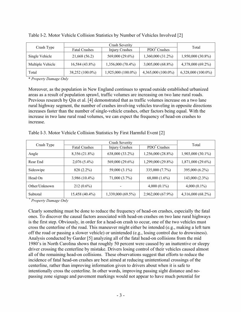
Total 38,252 (100.0%) 1,925,000 (100.0%) 4,365,000 (100.0%) 6,328,000 (100.0%) * Property Damage Only Two lane rural highways account for a substantial proportion of the highway network in New England, as well as the rest of the US. For example, in Maine roughly 95 percent of all rural highways have only two lanes, and according to Kalakota et al. [3], approximately 2.5 million miles, or 63 percent of US highway miles are on rural two-lane highways. Besides, 74.9 percent of fatalities occur on two lane rural highways, giving this highway type a higher fatality rate than all others (per vehicle mile traveled); for example, four to seven times higher than on rural interstate highways [3]. These facts demonstrate the importance of two lane highways in the research of transportation safety. Multi-vehicle crashes occur more often and generally cause more injury and property loss than single vehicle crashes (see Table I-2). Among multi-vehicle crash types, although head-on crashes are rare, they are responsible for a relatively large proportion of fatalities. Table I-3 shows motor vehicle collision statistics for 2003. Because there are some collisions with fixed or un-fixed objects, the subtotal of each category does not necessarily total to 100 percent. As shown in this table, head-on crashes accounted for less than 3 percent of all crashes in 2003, but these crashes were responsible for more than 10 percent of the fatal crashes.

- 3 -

Table I-2. Motor Vehicle Collision Statistics by Number of Vehicles Involved [2]

Crash Severity Crash Type Fatal Crashes Injury Crashes PDO* Crashes Total

Single Vehicle 21,668 (56.2) 569,000 (29.6%) 1,360,000 (31.2%) 1,950,000 (30.8%)

Multiple Vehicle 16,584 (43.8%) 1,356,000 (70.4%) 3,005,000 (68.8%) 4,378,000 (69.2%)

Total 38,252 (100.0%) 1,925,000 (100.0%) 4,365,000 (100.0%) 6,328,000 (100.0%) * Property Damage Only Moreover, as the population in New England continues to spread outside established urbanized areas as a result of population sprawl, traffic volumes are increasing on two lane rural roads. Previous research by Qin et al. [4] demonstrated that as traffic volumes increase on a two lane rural highway segment, the number of crashes involving vehicles traveling in opposite directions increases faster than the number of single-vehicle crashes, other factors being equal. With the increase in two lane rural road volumes, we can expect the frequency of head-on crashes to increase.

Table I-3. Motor Vehicle Collision Statistics by First Harmful Event [2]

Crash Severity Crash Type Fatal Crashes Injury Crashes PDO* Crashes Total

Angle 8,356 (21.8%) 638,000 (33.2%) 1,256,000 (28.8%) 1,903,000 (30.1%)

Rear End 2,076 (5.4%) 569,000 (29.6%) 1,299,000 (29.8%) 1,871,000 (29.6%)

Sideswipe 828 (2.2%) 59,000 (3.1%) 335,000 (7.7%) 395,000 (6.2%)

Head On 3,986 (10.4%) 71,000 (3.7%) 68,000 (1.6%) 143,000 (2.3%)

Other/Unknown 212 (0.6%) - 4,000 (0.1%) 4,000 (0.1%)

Subtotal 15,458 (40.4%) 1,339,000 (69.5%) 2,962,000 (67.9%) 4,316,000 (68.2%) * Property Damage Only Clearly something must be done to reduce the frequency of head-on crashes, especially the fatal ones. To discover the causal factors associated with head-on crashes on two lane rural highways is the first step. Obviously, in order for a head-on crash to occur, one of the two vehicles must cross the centerline of the road. This maneuver might either be intended (e.g., making a left turn off the road or passing a slower vehicle) or unintended (e.g., losing control due to drowsiness). Analysis conducted by Garder [5] analyzing all of the fatal head-on collisions from the mid 1980’s in North Carolina shows that roughly 50 percent were caused by an inattentive or sleepy driver crossing the centerline by mistake. Drivers losing control of their vehicles caused almost all of the remaining head-on collisions. These observations suggest that efforts to reduce the incidence of fatal head-on crashes are best aimed at reducing unintentional crossings of the centerline, rather than improving information given to drivers about when it is safe to intentionally cross the centerline. In other words, improving passing sight distance and no-passing zone signage and pavement markings would not appear to have much potential for

- 4 -

reducing the frequency of fatal head-on collisions. On the other hand, treatments such as installing centerline rumble strips or addition of a flush or raised median through horizontal curves (as has been done in several states across the country) may have more promise for reducing this type of crash. Another potential approach is to learn more about the exact features of the road environment that influence the severity of head-on crashes; that is, how and what causes a head-on crash to be fatal rather than non-fatal. This study focuses on two issues: investigating what roadway characteristics influence the incidence of head-on collisions, and analyzing the correlation between head-on crash severity and potential causality factors, such as the geometric characteristics of a road segment, weather conditions, road surface conditions, and time of occurrence using data collected on state-maintained two-lane roads in Connecticut. Identifying these correlated factors will help to better understand the crash phenomenon and in turn can result in safer roadway design standards. Objectives and Scope This report investigates how characteristics of two-lane rural highways affect the frequency and severity of head-on crashes, while controlling for characteristics of the vehicle, driver and occupants. The results provide valuable information for highway safety engineers to use for retrofitting existing highways and designing new highways to reduce the incidence of fatal head-on crashes. Consequently, the objective is to identify factors in the driving environment that help predict head-on crash severity on two lane rural highways to permit direct comparison among crashes. Severity is defined according to the highest level of injury experienced by the involved drivers. The injury level is measured on the KABCO scale [6], defined as follows

K = fatality; A = disabling injury, cannot leave the scene without assistance (i.e., broken bones, severe

wounds, unconsciousness, etc.); B = non-disabling injury, but visible (i.e., minor cuts, swelling, limping, bruises and

abrasions, etc.); C = probable injury, but not visible (i.e., complaint of pain or momentary

unconsciousness, etc.); O = no injury (property damage only).

Negative Binomial (NB) Generalized Linear Models (GLIM) were used to evaluate the effects of roadway geometric features on the incidence of head-on crashes. Ordered Probit modeling was used to estimate severity models using explanatory variables representing highway and crash characteristics. The analysis methods are discussed in more detail later in the document.

- 5 -

LITERATURE REVIEW Head-on Crashes in Rural Areas The 1999 statistics from the Fatality Analysis Reporting System (FARS) indicate that 18 percent of non-interchange, non-junction fatal crashes involved two vehicles colliding head-on. The percentage was the same for 1997 and 1998 data. In addition, these data reveal that [7]: • 75 percent of head-on crashes occur on rural roads, • 75 percent of head-on crashes occur on undivided two-lane roads, and • 83 percent of two-lane undivided road crashes occur on rural roads. In fact, the possibility of a fatality occurring during a head-on collision is three times higher in rural areas than in urban areas [8]. Zegeer et al. [9] found that although rates for other collisions generally increase as lane width increases, the frequency of run-off-road and opposite-direction collisions (including head-on crash and sideswipe collision) decrease. The most significant improvement occurs when widening lanes from 8 to 11 feet, where they found a reduction in head-on crashes of as much as 36 percent. Rates of property-damage and injury accidents decrease as lane width increases, corresponding to the overall accident rate for various lane widths. No changes in fatality rate occur as lane width changes; thus, no definite correlation was found between lane width and crash severity. In this research, they also found that increasing lane width resulted in a greater reduction in crash rates than the same increase in shoulder width. Moreover, alignment of the roadway affects the occurrence of head-on crashes, and the frequency of head-on crashes is usually higher on curved segments. Two other factors impacting head-on collisions are vehicle speed and no-passing zones. Most fatal head-on crashes take place on roadways with high posted speed limits [10]. Speed affects both the severity and the frequency of head-on collisions. Also, it was found in Kentucky that 25 percent of head-on collisions occur in no-passing zones [11]. Clissold [12] analyzed crash records in New Zealand and found that head-on collisions were over-represented in wet weather due to road surface conditions. On both urban and rural roads, an increase in head-on collision was observed on rainy days. These previous studies indicate that the frequency of head-on crashes, especially fatal head-on crashes, is much higher on undivided rural two-lane highways than other types of roadways. Also, the severity of head-on crashes is affected by some road segment characteristics, such as lane width, shoulder width, alignment, speed limit, passing restriction and road surface conditions. These findings are used in this study to provide a starting point for decisions about variables to be included in the study and preliminary analysis. Vehicle Crashes and Roadway Characteristics A number of researchers have investigated the empirical relationship between vehicle crashes (frequency and severity) and roadway characteristics. Although not all of them are directly applied to head-on crashes, their analysis perspectives could help us identify some more potential explanatory variables.

- 6 -

Agent and Deen [11] identified high-accident locations with respect to the functional type and geometry of the highway, using accident and volume data from rural highways in Kentucky collected from 1970 through 1972. They found that four-lane undivided highways had the highest accident, injury and fatality rates. Two-lane and three-lane highways had a significant percentage of head-on or opposite-direction sideswipe crashes. Also, two-lane highways had the highest percentage of crashes that occurred on curved segments. They used a severity index (SI), which is a weighted combination of KABCO scaled crash counts to compare the severity of different crash types, and found that the head-on crash is one of the most severe crash types. Chira-Chavala and Mak [13] found that sections with horizontal curvature greater than two degrees are overrepresented with regard to crash occurrence, much more so than time of day, weather and surface conditions or presence or absence of speeding. The combination of a sharp curve, wet conditions, and speeding contributed to accident overrepresentation. Al-Senan and Wright [8] conducted a discriminate analysis between two groups of sections: head-on crash sections (where more than three head-on crashes occurred during the analysis period) and control sections (the sections with similar characteristics with the head-on crash sections but no head-on crashes occurred during the analysis period) on rural two-lane roads with a volume of at least 2,000 vehicles per day. The proneness of a head-on section is significantly related to the following variables: the proportion of the section with pavement width of less than 24 ft, the weighted pavement width (which is defined as the summation of the products of width times length over which the width is uniform, divided by the total length, 1 mile), the proportion of the section with a shoulder width of less than 6 ft, the proportion of the section that is not level, the average speed limit of the section, the frequency of major access points on both sides and the frequency of reverse curves with zero tangents. This procedure also allowed for the quantification of head-on crash “proneness”, that is, assigning a probability level for the potentiality for a 1-mile section to have three head-on accidents in a 3-year period based on these roadway features. Garber and Graham [14] estimated time-series regression equations including policy variables, seasonal variables, and surrogate exposure variables for each of forty states using monthly FARS data from January 1976 through November 1988. The estimated results suggested a median increase in fatalities of 15 percent on rural Interstate highways, and 5 percent on non-Interstate roads where speed limits were raised. Miaou et al. [15] proposed a Poisson regression model to establish empirical relationships between truck accidents and key highway geometric design variables. Their final model suggests that annual average daily traffic (AADT) per lane, horizontal curvature, and vertical grade are significantly correlated with truck accident involvement rate, but the shoulder width has comparably less correlation. The curvature variables included in their best model are the mean absolute horizontal curvature and the mean absolute vertical grade, and both are positively correlated with truck crash frequency. Renski et al. [16] analyzed data describing single-vehicle crashes on Interstate highways in North Carolina using two methods: paired-comparison and ordered probit modeling. They found that there was a decrease in the probability of not being injured in a crash and an increase in the

- 7 -

probability of sustaining Class A, B, or C injuries (as defined in the introduction) on segments where speed limits increased from 55 mph to either 60 or 65 mph. Huang et al. [17] found that lane reduction (also known as a “road diet”), which here refers to the conversion of four-lane undivided roads into three-lane roads, can reduce crashes rate by 6 percent or less but has no significant influence on crash severity in a “before” and “after” study. Abdel-Aty [18] developed ordered probit models to predict the injury level of drivers for different types of locations using Florida vehicle crash data. He found curved segments to be significantly correlated with severe crashes. In this study, the author also estimated the severity level prediction model using nested logit modeling methodology. However, the nested logit approach does not significantly improve the goodness-of-fit of the models estimated using the ordered probit method. Given the difficulty of estimating nested logit models because of the large number of different nesting structures that need to be considered and based on the results of the various models estimated in this research, he indicated that the ordered probit models were easy to estimate and performed very well in modeling driver injury severity. These studies indicate that road segment characteristics could affect not only the frequency but also the severity of vehicle crashes. Different modeling methods were employed in estimating the empirical relationship between vehicle crashes (frequency and severity) and roadway characteristics. The potential correlated road characteristic variables are number of lanes, lane and shoulder width, speed limit, curvature and density of access points. Application to this Study Most of the research discussed above did not distinguish between head-on crashes and other types of crashes, especially in severity analysis. A few articles concerned mainly with head-on collisions are very old (before 1987). Nevertheless, this previous research provides important insight into statistical approaches for modeling relationships between highway features and geometry and highway safety, which helps us identify appropriate study methods.

- 8 -

STUDY DESIGN AND DATA COLLECTION For this research, we define a head-on crash as one involving two vehicles originally traveling in opposite directions, not including those involving turning vehicles. Opposite direction sideswipe collisions are also not included. The rest of this chapter describes how the analysis databases were compiled. Site Selection It is clear from basic physics and past research that impact speed is strongly correlated with crash severity [19]. Consequently, to help insure that vehicle speeds vary only within a distribution of free flow speeds at the locations where the crashes were observed, the head-on crashes considered for study were limited to those observed at locations with no traffic control on the main road. This was important because traffic signals and stop signs cause wider variations in speeds due to acceleration and deceleration patterns, rather than just natural variation due to driver behavior. In addition to traffic control, study sites were limited to two-lane highway sections. We also only chose sites where the cross-section is consistent through the segment—i.e., all segments have only one lane in each direction and have no passing lanes or turning lanes in either direction, and the lane and shoulder widths are constant through the segment. Also, none of the segments contain town centers or similar densely populated or developed areas, which may also introduce confounding factors. All segments have a uniform length of 1 km to remove segment length as a contributing factor. Within these constraints, segments were randomly selected from the Connecticut state highway network, with approximately equal numbers in east-west and north-south directions, to avoid bias due to sun glare. A total of 720 segments that satisfy the above criteria were gathered in the Connecticut dataset.

Photolog and PLV Software The physical characteristics of each segment were observed using the Connecticut Department of Transportation (ConnDOT) Photolog and Horizontal and Vertical Curve Classification and Display System (PLV-HC/VC) software. The Photolog is a roadway viewing system updated annually, on which the entire state-maintained roadway network containing approximately 6,155 route kilometers (12,300 photolog kilometers) is recorded with two Automatic Road Analyzer (ARAN) photolog systems. Each state-maintained highway in Connecticut may be viewed using the Photolog, which consists of images of the roadway taken every 0.01 km. The system consists of a set of forward-view Right-of-Way (ROW) images from the entire highway system, a set of side-view ROW images from one-half of the entire highway system, and a set of corresponding highway geometric data. The ConnDOT Photolog was used to obtain the speed limit, clear roadway width, number of access points and driveway type for each segment. Meanwhile, we gathered geometric characteristics such as the horizontal curvature and the vertical grade from the PLV-HC/VC Software. The PLV-HC/VC works in conjunction with the Photolog. While the ARAN van navigates the roadway to prepare the photolog, a mechanical recorder logs the trail of the vehicle and the elevation sequence as well. This software implements an algorithm developed by ConnDOT to process the ARAN horizontal and vertical alignment data. Thus we can get the

- 9 -

details of the horizontal and vertical curves from the PLV-HC/VC by specifying the start and end chainage of each analysis segment.

Roadway and Site Characteristics Previous research helped identify roadway and site characteristics that may be useful to estimate head-on crash severities. As a result, we observed lane width, shoulder width, centerline type, speed limit, and number of access points (including minor intersections and driveways by type) on all study sites. The number of access points is intended to represent the land use intensity, and type, in the case of driveways. A unique aspect of this research is the definition of variables to represent horizontal and vertical curves. Because the road sections are defined independently of the occurrence of horizontal and vertical curves, each section can contain more than one horizontal curve or vertical grade. Using these features for predicting highway crash incidence requires aggregation of the curve characteristics or disaggregation of the segments. In other words, one option is to create surrogate measures to aggregate the curvature and grade conditions along the length of a road section. A second option is to disaggregate those segments with multiple curves and grades into shorter sub-segments so that each subsegment contains a homogeneous combination of horizontal curvature and vertical grade [15]. The former is considered less direct from the engineering point of view and it may be more difficult for road designers to incorporate these measures into their current practice than the second method. However, because the location of a collision is often estimated and roughly assigned to the nearest milepost of the route on which it occurred, assigning vehicle accidents to road sections with lengths shorter than or close to the minimum difference between mile points is more susceptible to location error than assigning to longer road sections. Consequently, for this project we selected segments of 1 km in length and defined the following surrogate measures to characterize the curvature and grade conditions along the length of each:

1. Weighted mean of absolute horizontal and vertical curvature (WMAH and WMAV)

i

N

jjijii llWMAH ⎟⎟⎠

⎞⎜⎜⎝

⎛∆= ∑

=1,, (1)

i

N

jjijii lGlWMAV ⎟⎟⎠

⎞⎜⎜⎝

⎛= ∑

=1,, (2)

where il is the total length of segment i; N is the number of subsegments in segment i;

jil , is the length of subsegment j on segment i;

ji,∆ is the curve degree of subsegment j on segment i;

jiG , is the grade of subsegment j on segment i. These two parameters describe the entire segment for either horizontal or vertical curves. If either is close to zero, it indicates that the segment is close to a straight line with respect to that type of curvature. This would indicate the segment has a better sight distance, which may have mixed effects on safety. The improved sight distance would be expected to make it easier to

- 10 -

avoid collisions, but the monotony of a straight road may also lower drivers’ vigilance. If the value is relatively large, the segment could only have one curve with large radii and angle or a few sharp curves with shorter radii. Although these variables cannot separate these two cases well, they can represent whether or not the segment is generally straight or curvy (or overly undulating terrain).

2. Sum of absolute horizontal or vertical curvature change rate (SACRH and SACRV)

∑−

=+ ∆−∆=

1

1,1,

N

jjijiiSACRH (3)

∑−

=+ −=

1

1,1,

N

jjijii GGSACRV (4)

These variables account for the frequency of curvature changes on the segment, again for either horizontal or vertical curves. A larger SACRH or SACRV value means that vehicles driving on this segment must change steering angle more frequently, or must drive over many crests and sags, respectively. On the one hand, having to change steering more frequently may cause drivers to be more cautious to avoid collisions. But on the other hand, driving a long time on complex roadways may cause fatigue, and increase the risk of losing control of the vehicle.

3. Maximum absolute horizontal curvature or minimum grade change rate (MAXD and MINK)

{ }Niiii DDDMAXD ,2,1, ,,,max K= (5)

{ }Niiii KKKMINK ,2,1, ,,,min K= (6)

where jiD , is the degree of curve on sub-segment j on segment i;

jiK , is the rate of change in grade per unit length of subsegment j on segment i. The previously-defined variables may not always be able to account for a particularly dangerous case, for instance, a segment with one or two sharp horizontal or vertical curves. These two variables are designed to account for these possibilities.

4. Sum of combined horizontal and vertical curvature (CHV) ∑∑ +=

n

Sagn

m

Crestm CHVCHVCHV (7)

where mm

mCrestm K

CHV ω∆= (7a)

)2

( nHn

n

nsagn

LK

CHV ω−∆= (7b)

ωm is the distance between the crest of the vertical curve m and the mid-point of the corresponded horizontal curve; and

LHn is the length of the corresponded horizontal curve of vertical curve n. This variable is intended to be an effective single description of the combined horizontal and vertical curvature. The basis of the definition is identifying the difference between the mid-points of horizontal and vertical curves that overlap one another. We may expect that the degree to which the mid-point of the vertical curve is superimposed on the mid-point of the horizontal curve is a kind of index of coordination of the alignment. The function CHV (∆,K,ω) monotonically increases in the space of ),(),( ∞−∞∈∪−∈∆ ωππ and monotonically decreases

- 11 -

in the space of ),( ∞−∞∈K . Therefore, an increase in ∆ (a sharper turn) or ω (larger departure from the vertex of the vertical curve to the mid-point of the horizontal curve), and a decrease in K (a larger grade difference) all cause an increase in the value of CHV. In other words, a larger CHV is expected to indicate a more dangerous situation. Furthermore, CHV would not change if a segment were divided into several sub-segments, eliminating bias due to segment definitions.

Crash Database The ConnDOT Traffic Accident Viewing System (TAVS) program contains the crash data, consisting of detailed information about all crashes that occurred between January 1996 and December 2001 on all state maintained highways. The information from this database included the date, time, location, nature and the type of vehicles involved in each crash, as well as the type of crash. The following variables were extracted for each observation:

• Case Number: Each accident is identified by a unique case number. • Accident Location: Police reported chainage for each case. • Date of Accident: The date the crash occurred. • Time: The clock time that the crash occurred. • Light Condition: Ambient lighting state when the crash occurred (e.g. dark, dawn, dusk,

etc.) • Surface Condition: Roadway surface condition (e.g., wet, dry, icy, snow, sand, etc.) • Weather Condition: The weather at the time the crash occurred (e.g. fog, rain, snow,

hail, blowing, etc.) • Traffic Unit: Involved vehicle types (e.g. passenger car, van, truck. etc.) • Contributing Factor: Police reported causal factors (e.g. slippery surface, improper

passing maneuver, etc. • Crash Severity: Crash severities were coded on the KABCO scale: the classification of

an individual crash is defined by the most severe outcome experienced in the crash for each involved vehicle. A total of 228 head-on crashes occurring on the selected segments during the analysis

period were recorded in the Connecticut dataset.

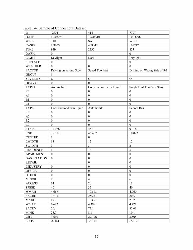
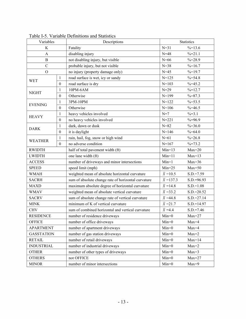
Data Aggregation The crash and segment datasets were merged into a single database. Each record contained variables such as vehicle type, light condition, weather, contributing factors, road surface condition and segment characteristics. Table I-4 gives a sample of crash entries in the database, and Table I-5 gives a list of the variables along with their definitions and some summary statistics.

- 12 -

Table I-4. Sample of Connecticut Dataset Id 2504 414 7707 DATE 10/03/96 12//08/01 10/16/96 WEEK THU SAT WED CASE# 158824 408347 161712 TIME 949 2332 823 DARK 0 1 0 LIGHT Daylight Dark Daylight SURFACE 0 1 0 WEATHER 0 0 0 FACTOR Driving on Wrong Side Speed Too Fast Driving on Wrong Side of Rd GROUP 1 1 1 SEVERITY O O O HEAVY 0 0 1 TYPE1 Automobile Construction/Farm Equip Single Unit Trk/2axle/4tire K1 0 0 0 A1 0 0 0 B1 0 0 0 C1 0 0 0 TYPE2 Construction/Farm Equip Automobile School Bus K2 0 0 0 A2 0 0 0 B2 0 0 0 C2 0 0 0 START 37.026 45.4 9.016 END 38.012 46.402 10.022 CENTER 1 0 1 LWIDTH 13 12 12 SWIDTH 3 3 2 RESIDENCE 1 16 5 APARTMENT 0 0 0 GAS_STATION 0 0 0 RETAIL 4 0 0 INDUSTRY 0 0 0 OFFICE 0 0 0 OTHER 0 0 0 MINOR 9 4 6 ACCESS 14 20 11 SPEED 40 35 40 WMAH 4.667 12.573 4.260 SACRH 64.5 255.4 80.5 MAXD 17.3 103.9 23.7 WMAV 0.682 4.399 4.421 SACRV 20.4 73.1 82.61 MINK 25.7 8.1 10.1 CHV 3.619 27.776 3.505 LCHV -6.344 -9.105 -22.12

- 13 -

Table I-5. Variable Definitions and Statistics Variables Descriptions Statistics

K Fatality N=31 %=13.6 A disabling injury N=48 %=21.1 B not disabling injury, but visible N=66 %=28.9 C probable injury, but not visible N=38 %=16.7 O no injury (property damage only) N=45 %=19.7

1 road surface is wet, icy or sandy N=125 %=54.8 WET

0 road surface is dry N=103 %=45.2 1 10PM-6AM N=29 %=12.7

NIGHT 0 Otherwise N=199 %=87.3 1 3PM-10PM N=122 %=53.5

EVENING 0 Otherwise N=106 %=46.5 1 heavy vehicles involved N=7 %=3.1

HEAVY 0 no heavy vehicles involved N=221 %=96.9 1 dark, dawn or dusk N=82 %=36.0

DARK 0 it is daylight N=146 %=64.0 1 rain, hail, fog, snow or high wind N=61 %=26.8

WEATHER 0 no adverse condition N=167 %=73.2

RWIDTH half of total pavement width (ft) Min=13 Max=20 LWIDTH one lane width (ft) Min=11 Max=13 ACCESS number of driveways and minor intersections Min=1 Max=36 SPEED speed limit (mph) Min=25 Max=50 WMAH weighted mean of absolute horizontal curvature x =10.5 S.D.=7.59 SACRH sum of absolute change rate of horizontal curvature x =137.3 S.D.=96.93 MAXD maximum absolute degree of horizontal curvature x =14.8 S.D.=1.08 WMAV weighted mean of absolute vertical curvature x =33.2 S.D.=20.52 SACRV sum of absolute change rate of vertical curvature x =44.8 S.D.=27.14 MINK minimum of K of vertical curvature x =21.7 S.D.=14.97 CHV sum of combined horizontal and vertical curvature x =4.4 S.D.=7.46 RESIDENCE number of residence driveways Min=0 Max=27 OFFICE number of office driveways Min=0 Max=4 APARTMENT number of apartment driveways Min=0 Max=4 GASSTATION number of gas station driveways Min=0 Max=2 RETAIL number of retail driveways Min=0 Max=14 INDUSTRIAL number of industrial driveways Min=0 Max=2 OTHER number of other types of driveways Min=0 Max=3 OTHERS not OFFICE Min=0 Max=27 MINOR number of minor intersections Min=0 Max=9

- 14 -

NEGATIVE BINOMIAL REGRESSION OF HEAD-ON CRASH INCIDENCE

Negative Binomial (NB) Generalized Linear Models (GLIM) In traffic safety research, GLIM has been more and more frequently adopted for estimation of crash prediction models because of its ability to relax the assumption of a normal distribution for the response variable. Instead, a GLIM framework using a Poisson-related distribution for the crash count is more appropriate, as it confirms to the non-negative and discrete nature of crash counts and leads to a more flexible discrete distribution form [20]. In a Poisson distributed case, the probability of observing ni crashes is represented as:

!i

mn

i nemp

i −

= , (8)

where m is the mean of the Poisson distribution, computed as NpnEm i == )( , (9)

with p being the probability of having a crash when the exposure is N. However, in realistic cases the mean under a Poisson distribution usually cannot represent the crash frequency Np at different observation sites. In fact, the real mean includes the average crash frequency and an error term following a Gamma distribution, due to the between site variation in the database [21]. In other words,

εNpem = , (10) assuming eε follows a Gamma distribution with mean 1 and variance δ [5]. Then the corresponding Poisson distribution is

!)()|(

i

Npen

ii neNpenP

iεε

ε−

= (11)

After integrating on ε for equation (4), the NB distribution is obtained as in

i

ii Np

NpNpn

nnP ⎟⎟⎠

⎞⎜⎜⎝

⎛+⎟⎟

⎠

⎞⎜⎜⎝

⎛+Γ+Γ

+Γ=

θθθ

θθ

θ

)()1()()( , (12)

where θ is the inverse of the dispersion parameter k in the NB distribution [5]. Instead of being equal to the mean, the variance of the NB distribution is

2)( kmmnVar i += . (13) When k is not significantly different from 0, the NB distribution is approximately equivalent to a Poisson distribution. Many previous studies have applied NB GLIM in highway crash analysis under different circumstances. Wang and Nihan used NB GLIM to estimate bicycle-motor vehicle (BMV) crashes at intersections in the Tokyo metropolitan area [5]. Shankar et al. also adopted NB GLIM in modeling the effects of roadway geometric and environmental features on freeway safety [22]. Miaou evaluated the performance of negative binomial regression models in establishing the relationship between truck crash and geometry design of road segments [23]. In this paper, the head-on crash count (Hcrash) is assumed to have a negative binomial distribution, and the total vehicle-kilometers-traveled (VKT) in six years for each segment is used as the exposure. A logarithmic function is used to link the expectation of the distribution of Hcrash and

- 15 -

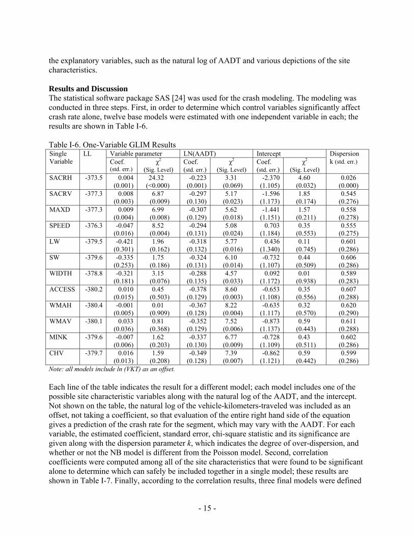
the explanatory variables, such as the natural log of AADT and various depictions of the site characteristics. Results and Discussion The statistical software package SAS [24] was used for the crash modeling. The modeling was conducted in three steps. First, in order to determine which control variables significantly affect crash rate alone, twelve base models were estimated with one independent variable in each; the results are shown in Table I-6. Table I-6. One-Variable GLIM Results

Variable parameter LN(AADT) Intercept Single Variable

LL Coef. (std. err.)

χ2 (Sig. Level)

Coef. (std. err.)

χ2 (Sig. Level)

Coef. (std. err.)

χ2 (Sig. Level)

Dispersion k (std. err.)

SACRH -373.5 0.004 (0.001)

24.32 (<0.000)

-0.223 (0.001)

3.31 (0.069)

-2.370 (1.105)

4.60 (0.032)

0.026 (0.000)

SACRV -377.3 0.008 (0.003)

6.87 (0.009)

-0.297 (0.130)

5.17 (0.023)

-1.596 (1.173)

1.85 (0.174)

0.545 (0.276)

MAXD -377.3 0.009 (0.004)

6.99 (0.008)

-0.307 (0.129)

5.62 (0.018)

-1.441 (1.151)

1.57 (0.211)

0.558 (0.278)

SPEED -376.3 -0.047 (0.016)

8.52 (0.004)

-0.294 (0.131)

5.08 (0.024)

0.703 (1.184)

0.35 (0.553)

0.555 (0.275)

LW -379.5 -0.421 (0.301)

1.96 (0.162)

-0.318 (0.132)

5.77 (0.016)

0.436 (1.340)

0.11 (0.745)

0.601 (0.286)

SW -379.6 -0.335 (0.253)

1.75 (0.186)

-0.324 (0.131)

6.10 (0.014)

-0.732 (1.107)

0.44 (0.509)

0.606 (0.286)

WIDTH -378.8 -0.321 (0.181)

3.15 (0.076)

-0.288 (0.135)

4.57 (0.033)

0.092 (1.172)

0.01 (0.938)

0.589 (0.283)

ACCESS -380.2 0.010 (0.015)

0.45 (0.503)

-0.378 (0.129)

8.60 (0.003)

-0.653 (1.108)

0.35 (0.556)

0.607 (0.288)

WMAH -380.4 -0.001 (0.005)

0.01 (0.909)

-0.367 (0.128)

8.22 (0.004)

-0.635 (1.117)

0.32 (0.570)

0.620 (0.290)

WMAV -380.1 0.033 (0.036)

0.81 (0.368)

-0.352 (0.129)

7.52 (0.006)

-0.873 (1.137)

0.59 (0.443)

0.611 (0.288)

MINK -379.6 -0.007 (0.006)

1.62 (0.203)

-0.337 (0.130)

6.77 (0.009)

-0.728 (1.109)

0.43 (0.511)

0.602 (0.286)

CHV -379.7 0.016 (0.013)

1.59 (0.208)

-0.349 (0.128)

7.39 (0.007)

-0.862 (1.121)

0.59 (0.442)

0.599 (0.286)

Note: all models include ln (VKT) as an offset. Each line of the table indicates the result for a different model; each model includes one of the possible site characteristic variables along with the natural log of the AADT, and the intercept. Not shown on the table, the natural log of the vehicle-kilometers-traveled was included as an offset, not taking a coefficient, so that evaluation of the entire right hand side of the equation gives a prediction of the crash rate for the segment, which may vary with the AADT. For each variable, the estimated coefficient, standard error, chi-square statistic and its significance are given along with the dispersion parameter k, which indicates the degree of over-dispersion, and whether or not the NB model is different from the Poisson model. Second, correlation coefficients were computed among all of the site characteristics that were found to be significant alone to determine which can safely be included together in a single model; these results are shown in Table I-7. Finally, according to the correlation results, three final models were defined

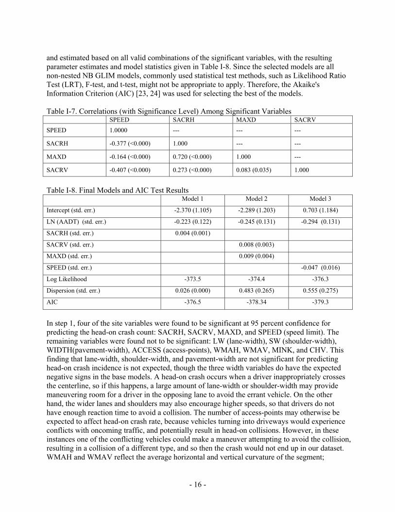
- 16 -

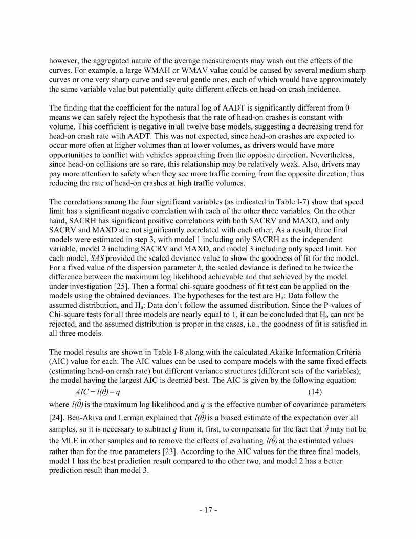
and estimated based on all valid combinations of the significant variables, with the resulting parameter estimates and model statistics given in Table I-8. Since the selected models are all non-nested NB GLIM models, commonly used statistical test methods, such as Likelihood Ratio Test (LRT), F-test, and t-test, might not be appropriate to apply. Therefore, the Akaike's Information Criterion (AIC) [23, 24] was used for selecting the best of the models. Table I-7. Correlations (with Significance Level) Among Significant Variables SPEED SACRH MAXD SACRV SPEED 1.0000 --- --- ---

SACRH -0.377 (<0.000) 1.000 --- ---

MAXD -0.164 (<0.000) 0.720 (<0.000) 1.000 ---

SACRV -0.407 (<0.000) 0.273 (<0.000) 0.083 (0.035) 1.000

Table I-8. Final Models and AIC Test Results Model 1 Model 2 Model 3

Intercept (std. err.) -2.370 (1.105) -2.289 (1.203) 0.703 (1.184)

LN (AADT) (std. err.) -0.223 (0.122) -0.245 (0.131) -0.294 (0.131)

SACRH (std. err.) 0.004 (0.001)

SACRV (std. err.) 0.008 (0.003)

MAXD (std. err.) 0.009 (0.004)

SPEED (std. err.) -0.047 (0.016)

Log Likelihood -373.5 -374.4 -376.3

Dispersion (std. err.) 0.026 (0.000) 0.483 (0.265) 0.555 (0.275)

AIC -376.5 -378.34 -379.3

In step 1, four of the site variables were found to be significant at 95 percent confidence for predicting the head-on crash count: SACRH, SACRV, MAXD, and SPEED (speed limit). The remaining variables were found not to be significant: LW (lane-width), SW (shoulder-width), WIDTH(pavement-width), ACCESS (access-points), WMAH, WMAV, MINK, and CHV. This finding that lane-width, shoulder-width, and pavement-width are not significant for predicting head-on crash incidence is not expected, though the three width variables do have the expected negative signs in the base models. A head-on crash occurs when a driver inappropriately crosses the centerline, so if this happens, a large amount of lane-width or shoulder-width may provide maneuvering room for a driver in the opposing lane to avoid the errant vehicle. On the other hand, the wider lanes and shoulders may also encourage higher speeds, so that drivers do not have enough reaction time to avoid a collision. The number of access-points may otherwise be expected to affect head-on crash rate, because vehicles turning into driveways would experience conflicts with oncoming traffic, and potentially result in head-on collisions. However, in these instances one of the conflicting vehicles could make a maneuver attempting to avoid the collision, resulting in a collision of a different type, and so then the crash would not end up in our dataset. WMAH and WMAV reflect the average horizontal and vertical curvature of the segment;

- 17 -

however, the aggregated nature of the average measurements may wash out the effects of the curves. For example, a large WMAH or WMAV value could be caused by several medium sharp curves or one very sharp curve and several gentle ones, each of which would have approximately the same variable value but potentially quite different effects on head-on crash incidence. The finding that the coefficient for the natural log of AADT is significantly different from 0 means we can safely reject the hypothesis that the rate of head-on crashes is constant with volume. This coefficient is negative in all twelve base models, suggesting a decreasing trend for head-on crash rate with AADT. This was not expected, since head-on crashes are expected to occur more often at higher volumes than at lower volumes, as drivers would have more opportunities to conflict with vehicles approaching from the opposite direction. Nevertheless, since head-on collisions are so rare, this relationship may be relatively weak. Also, drivers may pay more attention to safety when they see more traffic coming from the opposite direction, thus reducing the rate of head-on crashes at high traffic volumes. The correlations among the four significant variables (as indicated in Table I-7) show that speed limit has a significant negative correlation with each of the other three variables. On the other hand, SACRH has significant positive correlations with both SACRV and MAXD, and only SACRV and MAXD are not significantly correlated with each other. As a result, three final models were estimated in step 3, with model 1 including only SACRH as the independent variable, model 2 including SACRV and MAXD, and model 3 including only speed limit. For each model, SAS provided the scaled deviance value to show the goodness of fit for the model. For a fixed value of the dispersion parameter k, the scaled deviance is defined to be twice the difference between the maximum log likelihood achievable and that achieved by the model under investigation [25]. Then a formal chi-square goodness of fit test can be applied on the models using the obtained deviances. The hypotheses for the test are Ho: Data follow the assumed distribution, and Ha: Data don’t follow the assumed distribution. Since the P-values of Chi-square tests for all three models are nearly equal to 1, it can be concluded that Ho can not be rejected, and the assumed distribution is proper in the cases, i.e., the goodness of fit is satisfied in all three models. The model results are shown in Table I-8 along with the calculated Akaike Information Criteria (AIC) value for each. The AIC values can be used to compare models with the same fixed effects (estimating head-on crash rate) but different variance structures (different sets of the variables); the model having the largest AIC is deemed best. The AIC is given by the following equation:

q)θl(AIC −= ˆ (14) where )θl( ˆ is the maximum log likelihood and q is the effective number of covariance parameters [24]. Ben-Akiva and Lerman explained that )θl( ˆ is a biased estimate of the expectation over all samples, so it is necessary to subtract q from it, first, to compensate for the fact that θ̂ may not be the MLE in other samples and to remove the effects of evaluating )θl( ˆ at the estimated values rather than for the true parameters [23]. According to the AIC values for the three final models, model 1 has the best prediction result compared to the other two, and model 2 has a better prediction result than model 3.

- 18 -

Speed limit is commonly found to influence crash rates with a negative coefficient, as found here. It is important to remember that the speed limit on a road is not the same as the average travel speed on the road. This negative effect is usually considered to be due to roads with high crash frequencies being assigned lower speed limits as a safety precaution, or because the speed limit is often set according to the design speed, which is lower on roads with poor geometry due to the reduced sight distance. Predicting head-on crash incidence due to the combined effects of SACRV and MAXD, model 2 shows that the number of crashes increases with both variables. This suggests that the combination of an undulating vertical alignment (i.e., many crests and sags, one after another), combined with at least one sharp horizontal curve increases the risk of a head-on crash occurring. This makes sense, as such a vertical alignment likely reduces the sight distance considerably, permitting oncoming vehicles to momentarily disappear and suddenly reappear in the driver’s field of vision, and a very sharp horizontal curve presents a challenging task to the driver. Model 1, with SACRH, has the best prediction result, and shows an increasing trend in the incidence of head-on crashes with the sum of the absolute rates of change of the horizontal alignment. This is also an expected result, for two reasons. First, similar to the corresponding measure for vertical curves, a winding road may cause oncoming vehicles to disappear from the driver’s field of vision. Second, constantly having to change steering direction in response to so many changes in the horizontal curvature may overtax drivers and push them beyond their ability to safely negotiate the road segment. This finding confirms the conjecture by Hauer that crashes are associated mainly with curve entry and exit [26]. While he found no clear evidence of this, his investigations did find that the larger the degree of horizontal curve, the more crashes occur along the curve. This is consistent with the finding here about the effect of MAXD on the incidence of head-on crashes.

- 19 -

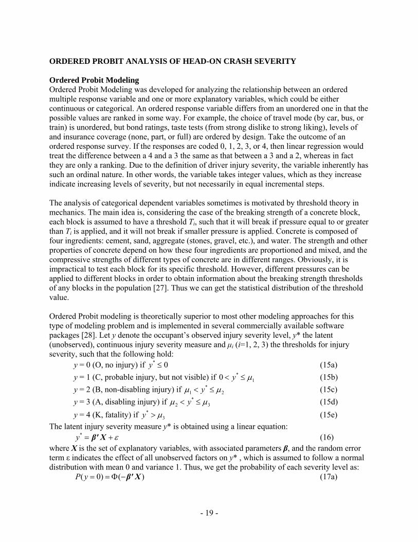
ORDERED PROBIT ANALYSIS OF HEAD-ON CRASH SEVERITY Ordered Probit Modeling Ordered Probit Modeling was developed for analyzing the relationship between an ordered multiple response variable and one or more explanatory variables, which could be either continuous or categorical. An ordered response variable differs from an unordered one in that the possible values are ranked in some way. For example, the choice of travel mode (by car, bus, or train) is unordered, but bond ratings, taste tests (from strong dislike to strong liking), levels of and insurance coverage (none, part, or full) are ordered by design. Take the outcome of an ordered response survey. If the responses are coded 0, 1, 2, 3, or 4, then linear regression would treat the difference between a 4 and a 3 the same as that between a 3 and a 2, whereas in fact they are only a ranking. Due to the definition of driver injury severity, the variable inherently has such an ordinal nature. In other words, the variable takes integer values, which as they increase indicate increasing levels of severity, but not necessarily in equal incremental steps. The analysis of categorical dependent variables sometimes is motivated by threshold theory in mechanics. The main idea is, considering the case of the breaking strength of a concrete block, each block is assumed to have a threshold Ti, such that it will break if pressure equal to or greater than Ti is applied, and it will not break if smaller pressure is applied. Concrete is composed of four ingredients: cement, sand, aggregate (stones, gravel, etc.), and water. The strength and other properties of concrete depend on how these four ingredients are proportioned and mixed, and the compressive strengths of different types of concrete are in different ranges. Obviously, it is impractical to test each block for its specific threshold. However, different pressures can be applied to different blocks in order to obtain information about the breaking strength thresholds of any blocks in the population [27]. Thus we can get the statistical distribution of the threshold value. Ordered Probit modeling is theoretically superior to most other modeling approaches for this type of modeling problem and is implemented in several commercially available software packages [28]. Let y denote the occupant’s observed injury severity level, y* the latent (unobserved), continuous injury severity measure and µi (i=1, 2, 3) the thresholds for injury severity, such that the following hold:

y = 0 (O, no injury) if 0* ≤y (15a) y = 1 (C, probable injury, but not visible) if 1

*0 µ≤< y (15b) y = 2 (B, non-disabling injury) if 2

*1 µµ ≤< y (15c)

y = 3 (A, disabling injury) if 3*

2 µµ ≤< y (15d) y = 4 (K, fatality) if 3

* µ>y (15e) The latent injury severity measure y* is obtained using a linear equation:

ε+= Xβ'*y (16) where X is the set of explanatory variables, with associated parameters β, and the random error term ε indicates the effect of all unobserved factors on y* , which is assumed to follow a normal distribution with mean 0 and variance 1. Thus, we get the probability of each severity level as:

)()0( Xβ'−Φ==yP (17a)

- 20 -

)()()1( 1 Xβ'Xβ' −Φ−−Φ== µyP (17b) )()()2( 12 Xβ'Xβ' −Φ−−Φ== µµyP (17c) )()()3( 23 Xβ'Xβ' −Φ−−Φ== µµyP (17d)

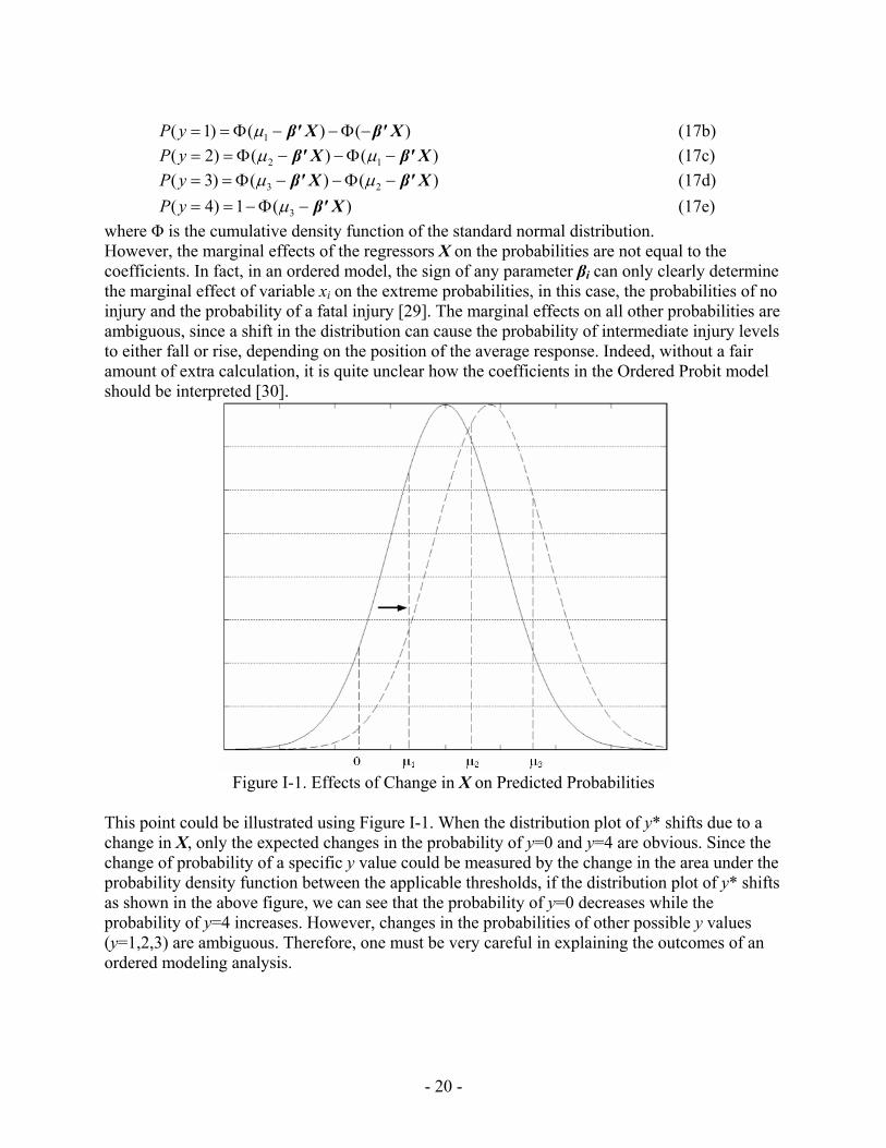
)(1)4( 3 Xβ'−Φ−== µyP (17e) where Φ is the cumulative density function of the standard normal distribution. However, the marginal effects of the regressors X on the probabilities are not equal to the coefficients. In fact, in an ordered model, the sign of any parameter βi can only clearly determine the marginal effect of variable xi on the extreme probabilities, in this case, the probabilities of no injury and the probability of a fatal injury [29]. The marginal effects on all other probabilities are ambiguous, since a shift in the distribution can cause the probability of intermediate injury levels to either fall or rise, depending on the position of the average response. Indeed, without a fair amount of extra calculation, it is quite unclear how the coefficients in the Ordered Probit model should be interpreted [30].

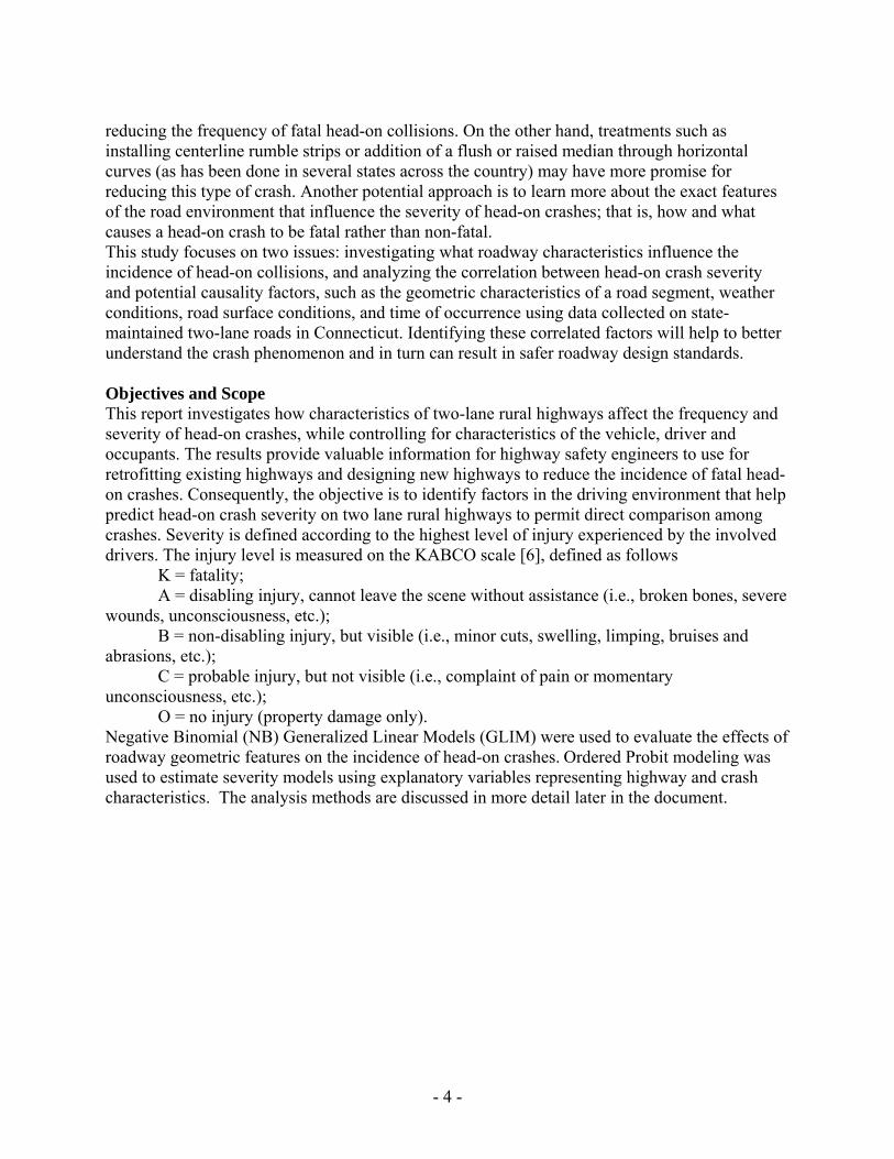
Figure I-1. Effects of Change in X on Predicted Probabilities

This point could be illustrated using Figure I-1. When the distribution plot of y* shifts due to a change in X, only the expected changes in the probability of y=0 and y=4 are obvious. Since the change of probability of a specific y value could be measured by the change in the area under the probability density function between the applicable thresholds, if the distribution plot of y* shifts as shown in the above figure, we can see that the probability of y=0 decreases while the probability of y=4 increases. However, changes in the probabilities of other possible y values (y=1,2,3) are ambiguous. Therefore, one must be very careful in explaining the outcomes of an ordered modeling analysis.

- 21 -

Model Selection The goodness of fit for different models estimated from the same set of data can be compared using either the likelihood ratio statistic (LRS) or Akaike’s Information Criterion (AIC). The LRS is only applicable with nested models, that is, when one model is a restricted version of the other, where a restriction indicates that one or more coefficients are removed or identical to one another. The form of the test is given by

⎟⎟⎠

⎞⎜⎜⎝

⎛−=

)ˆ()ˆ(ln2

θθ

u

r

LLLRS (18)

where )ˆ(θrL is the likelihood value of the restricted model (r) and the )ˆ(θuL is the likelihood value of the unrestricted model (u). The test statistic is distributed as a chi-squared random variable, with degrees of freedom equal to the difference in the number of parameters between the two models. AIC is useful for both nested and non-nested models. The model yielding the smallest value of AIC is estimated to be the “closest” to the unknown truth, among the candidate models considered.

KLAIC 2))ˆ(ln(2 +−= θ (19) where K is the number of free parameters in the model. However, the AIC criterion may perform poorly if there are too many parameters in relation to the size of the sample. Sugiura [31] derived a small-sample (second order) expression which leads to a refined criterion denoted as AICc,

1)1(22))ˆ(log(2

−−+

++−=KnKKKLAICC θ (20)

or

1)1(2

−−+

+=KnKKAICAICC (21)

where n is the sample size. Generally, AICc is recommended when the ratio n/K is small (say < 40).

Crash Characteristics Model Intuitively, the crash-related factors recorded in the police reports are very important in crash severity prediction. Those factors are temporal in nature, and describe the prevailing conditions under which the crash occurred. In this study, the crash-related factors are light condition, surface condition, weather condition, time of day and the type of involved vehicles. As these variables vary, it is expected the driver behaviors and the vehicle mechanical performance will also change, thus when a head-on crash unfortunately happens, the crash severity level may become different. For example, it is more difficult to control a vehicle on an icy or wet road surface than in normal conditions, so impact speeds may be greater. In addition, one may feel drowsy at midnight, so reaction time becomes longer, allowing less time to slow the vehicle when attempting to avoid a collision. In both of these cases the impact speed may be higher, and the severity level may also be higher keeping other conditions the same.

- 22 -

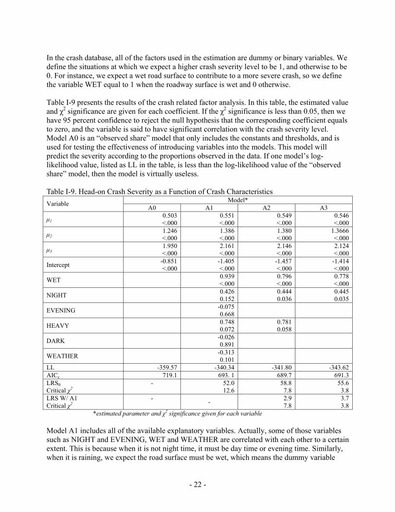
In the crash database, all of the factors used in the estimation are dummy or binary variables. We define the situations at which we expect a higher crash severity level to be 1, and otherwise to be 0. For instance, we expect a wet road surface to contribute to a more severe crash, so we define the variable WET equal to 1 when the roadway surface is wet and 0 otherwise. Table I-9 presents the results of the crash related factor analysis. In this table, the estimated value and χ2 significance are given for each coefficient. If the χ2 significance is less than 0.05, then we have 95 percent confidence to reject the null hypothesis that the corresponding coefficient equals to zero, and the variable is said to have significant correlation with the crash severity level. Model A0 is an “observed share” model that only includes the constants and thresholds, and is used for testing the effectiveness of introducing variables into the models. This model will predict the severity according to the proportions observed in the data. If one model’s log-likelihood value, listed as LL in the table, is less than the log-likelihood value of the “observed share” model, then the model is virtually useless. Table I-9. Head-on Crash Severity as a Function of Crash Characteristics

Model* Variable A0 A1 A2 A3

µ1 0.503 <.000

0.551 <.000

0.549 <.000

0.546 <.000

µ2 1.246 <.000

1.386 <.000

1.380 <.000

1.3666 <.000

µ3 1.950 <.000

2.161 <.000

2.146 <.000

2.124 <.000

Intercept -0.851 <.000

-1.405 <.000

-1.457 <.000

-1.414 <.000

WET 0.939 <.000

0.796 <.000

0.778 <.000

NIGHT 0.426 0.152

0.444 0.036

0.445 0.035

EVENING -0.075 0.668

HEAVY 0.748 0.072

0.781 0.058

DARK -0.026 0.891

WEATHER -0.313 0.101

LL -359.57 -340.34 -341.80 -343.62 AICc 719.1 693. 1 689.7 691.3LRS0 Critical χ2

- 52.0 12.6

58.8 7.8

55.6 3.8

LRS W/ A1 Critical χ2

- - 2.9 7.8

3.7 3.8

*estimated parameter and χ2 significance given for each variable Model A1 includes all of the available explanatory variables. Actually, some of those variables such as NIGHT and EVENING, WET and WEATHER are correlated with each other to a certain extent. This is because when it is not night time, it must be day time or evening time. Similarly, when it is raining, we expect the road surface must be wet, which means the dummy variable

- 23 -

WET equals to 1. If some of the explanatory variables in the same model are correlated, the estimated coefficients might fail to reveal the real marginal effect of the predictor variables on the dependent variable. Consequently, Model A2 drops some insignificant variables but retains WET, NIGHT and HEAVY. Model A3 drops HEAVY which is not significant at 95 percent confidence, although the AICc value for A3 does not indicate it to be superior to Model A2. Therefore, this round of estimation reflects that that WET and NIGHT are both significant at a 95 percent confidence level, HEAVY is not as significant as those two but rather close to a 95 percent confidence level while EVENING, DARK and WEATHER were found to be poor predictors. Using the AICc and LRS statistic, we select model A2 as the base model for the next step in the analysis.

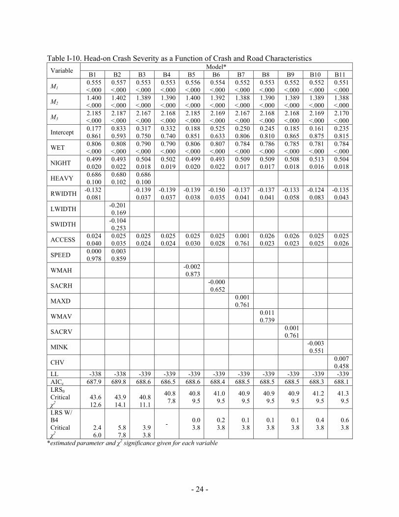
Models including Roadway Segment Characteristics We next tested the effect of segment characteristics on head-on crash severity. To the crash characteristics model obtained previously (Model A2) we add segment characteristic variables. Those variables include geometric characteristics such as lane width, shoulder width, the measures of horizontal and vertical curves discussed in detail before, the number of access points including minor-intersections and driveways, and the speed limit. The speed limit is inherently a composite reflection of the segment characteristics, for it is usually selected according to the sight distance, lane width, shoulder width, and perhaps safety experience. So we expect that significant correlations will be found among these segment characteristic variables. In the estimation procedure, we intended to avoid including highly correlated variables in the same model. The model estimation results are presented in Table I-10. Models B1 and B2 are designed to investigate the effect of pavement width on the head-on crash severity. The variable RWIDTH accounts for the entire paved road surface width in each direction, and is equal to the sum of the lane width (LWIDTH) and the shoulder width (SWIDTH). Model B1 has a smaller AICc value than Model B2, suggesting that RWIDTH is more significant than the separated relevant parts. This suggests that on two lane highways, the effect on safety does not differentiate between the lane and the shoulder, and only the available roadway width is important. From Model B1 through B3, we find that along with the newly introduced segment variables, the HEAVY variable is no longer as significant as before. So Model B4 drops HEAVY, and serves as the comparison basis for this group of models. From Model B4 to B11, we introduce one horizontal and vertical curve measure into the model at a time. However, none of the curve measures are significant at a 95 percent confidence level.

- 24 -

Table I-10. Head-on Crash Severity as a Function of Crash and Road Characteristics Model* Variable B1 B2 B3 B4 B5 B6 B7 B8 B9 B10 B11

Μ1 0.555 <.000

0.557 <.000

0.553 <.000

0.553 <.000

0.556 <.000

0.554 <.000

0.552 <.000

0.553 <.000

0.552 <.000

0.552 <.000

0.551 <.000

Μ2 1.400 <.000

1.402 <.000

1.389 <.000

1.390 <.000

1.400 <.000

1.392 <.000

1.388 <.000

1.390 <.000

1.389 <.000

1.389 <.000

1.388 <.000

Μ3 2.185 <.000

2.187 <.000

2.167 <.000

2.168 <.000

2.185 <.000

2.169 <.000

2.167 <.000

2.168 <.000

2.168 <.000

2.169 <.000

2.170 <.000

Intercept 0.177 0.861

0.833 0.593

0.317 0.750

0.332 0.740

0.188 0.851

0.525 0.633

0.250 0.806

0.245 0.810

0.185 0.865

0.161 0.875

0.235 0.815

WET 0.806 <.000

0.808 <.000

0.790 <.000

0.790 <.000

0.806 <.000

0.807 <.000

0.784 <.000

0.786 <.000

0.785 <.000

0.781 <.000

0.784 <.000

NIGHT 0.499 0.020

0.493 0.022

0.504 0.018

0.502 0.019

0.499 0.020

0.493 0.022

0.509 0.017

0.509 0.017

0.508 0.018

0.513 0.016

0.504 0.018

HEAVY 0.686 0.100

0.680 0.102

0.686 0.100

RWIDTH -0.132 0.081 -0.139

0.037 -0.139 0.037

-0.139 0.038

-0.150 0.035

-0.137 0.041

-0.137 0.041

-0.133 0.058

-0.124 0.083

-0.135 0.043

LWIDTH -0.201 0.169

SWIDTH -0.104 0.253

ACCESS 0.024 0.040

0.025 0.035

0.025 0.024

0.025 0.024

0.025 0.030

0.025 0.028

0.001 0.761

0.026 0.023

0.026 0.023

0.025 0.025

0.025 0.026

SPEED 0.000 0.978

0.003 0.859

WMAH -0.002 0.873

SACRH -0.000 0.652

MAXD 0.001 0.761

WMAV 0.011 0.739

SACRV 0.001 0.761

MINK -0.003 0.551

CHV 0.007 0.458

LL -338 -338 -339 -339 -339 -339 -339 -339 -339 -339 -339 AICc 687.9 689.8 688.6 686.5 688.6 688.4 688.5 688.5 688.5 688.3 688.1LRS0 Critical χ2

43.6 12.6

43.9 14.1

40.8 11.1

40.8 7.8

40.8 9.5

41.0 9.5

40.9 9.5

40.9 9.5

40.9 9.5

41.2 9.5

41.3 9.5

LRS W/ B4 Critical χ2

2.4 6.0

5.8 7.8

3.9 3.8

- 0.0 3.8

0.2 3.8

0.1 3.8

0.1 3.8

0.1 3.8

0.4 3.8

0.6 3.8

*estimated parameter and χ2 significance given for each variable

- 25 -

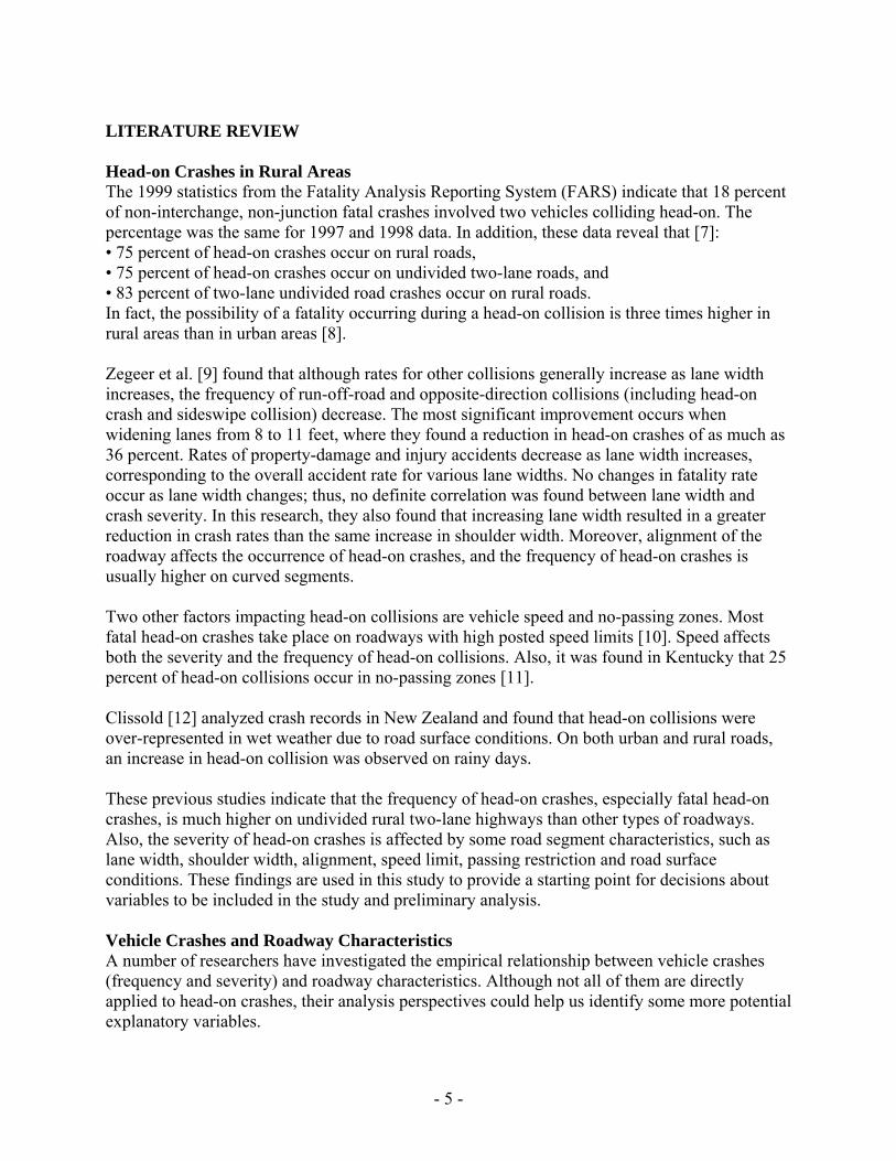
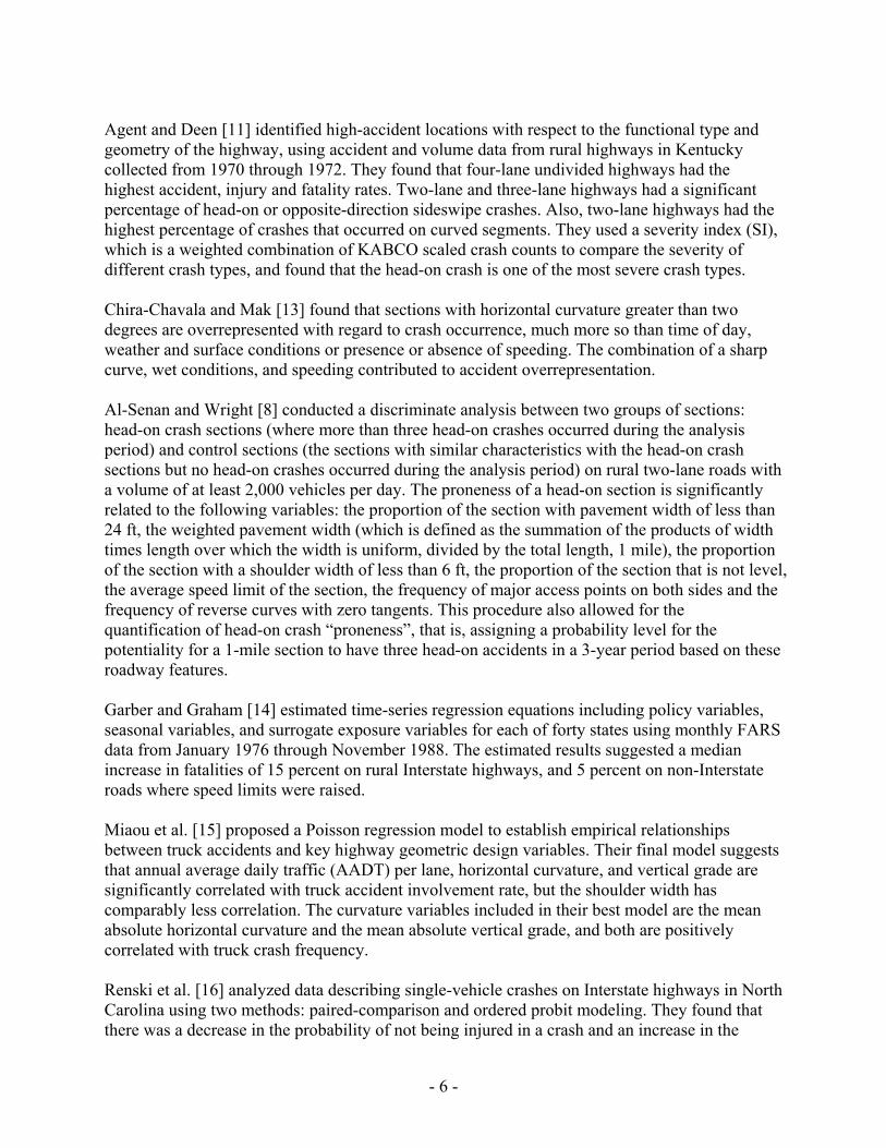
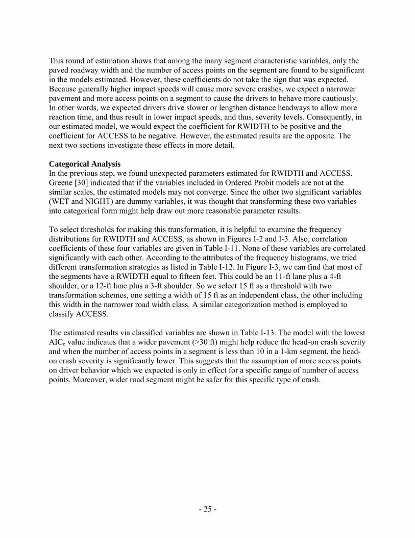
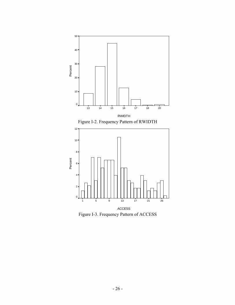
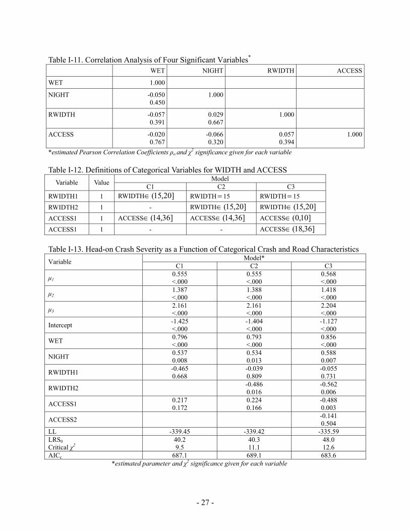
This round of estimation shows that among the many segment characteristic variables, only the paved roadway width and the number of access points on the segment are found to be significant in the models estimated. However, these coefficients do not take the sign that was expected. Because generally higher impact speeds will cause more severe crashes, we expect a narrower pavement and more access points on a segment to cause the drivers to behave more cautiously. In other words, we expected drivers drive slower or lengthen distance headways to allow more reaction time, and thus result in lower impact speeds, and thus, severity levels. Consequently, in our estimated model, we would expect the coefficient for RWIDTH to be positive and the coefficient for ACCESS to be negative. However, the estimated results are the opposite. The next two sections investigate these effects in more detail. Categorical Analysis In the previous step, we found unexpected parameters estimated for RWIDTH and ACCESS. Greene [30] indicated that if the variables included in Ordered Probit models are not at the similar scales, the estimated models may not converge. Since the other two significant variables (WET and NIGHT) are dummy variables, it was thought that transforming these two variables into categorical form might help draw out more reasonable parameter results. To select thresholds for making this transformation, it is helpful to examine the frequency distributions for RWIDTH and ACCESS, as shown in Figures I-2 and I-3. Also, correlation coefficients of these four variables are given in Table I-11. None of these variables are correlated significantly with each other. According to the attributes of the frequency histograms, we tried different transformation strategies as listed in Table I-12. In Figure I-3, we can find that most of the segments have a RWIDTH equal to fifteen feet. This could be an 11-ft lane plus a 4-ft shoulder, or a 12-ft lane plus a 3-ft shoulder. So we select 15 ft as a threshold with two transformation schemes, one setting a width of 15 ft as an independent class, the other including this width in the narrower road width class. A similar categorization method is employed to classify ACCESS. The estimated results via classified variables are shown in Table I-13. The model with the lowest AICc value indicates that a wider pavement (>30 ft) might help reduce the head-on crash severity and when the number of access points in a segment is less than 10 in a 1-km segment, the head-on crash severity is significantly lower. This suggests that the assumption of more access points on driver behavior which we expected is only in effect for a specific range of number of access points. Moreover, wider road segment might be safer for this specific type of crash.

- 26 -

RWIDTH

20181716151413

Perc

ent

50

40

30

20

10

0

Figure I-2. Frequency Pattern of RWIDTH

ACCESS

26211713951

Perc

ent

12

10

8

6

4

2

0

Figure I-3. Frequency Pattern of ACCESS

- 27 -

Table I-11. Correlation Analysis of Four Significant Variables* WET NIGHT RWIDTH ACCESS

WET 1.000

NIGHT -0.0500.450

1.000

RWIDTH -0.0570.391

0.0290.667

1.000

ACCESS -0.0200.767

-0.0660.320

0.057 0.394

1.000

*estimated Pearson Correlation Coefficients ρo and χ2 significance given for each variable Table I-12. Definitions of Categorical Variables for WIDTH and ACCESS

Model Variable Value C1 C2 C3 RWIDTH1 1 RWIDTH ]20,15(∈ RWIDTH= 15 RWIDTH= 15

RWIDTH2 1 - RWIDTH ]20,15(∈ RWIDTH ]20,15(∈

ACCESS1 1 ACCESS ]36,14(∈ ACCESS ]36,14(∈ ACCESS ]10,0(∈

ACCESS1 1 - - ACCESS ]36,18(∈

Table I-13. Head-on Crash Severity as a Function of Categorical Crash and Road Characteristics

Model* Variable C1 C2 C3

µ1 0.555 <.000

0.555 <.000

0.568 <.000

µ2 1.387 <.000

1.388 <.000

1.418 <.000

µ3 2.161 <.000

2.161 <.000

2.204 <.000

Intercept -1.425 <.000

-1.404 <.000

-1.127 <.000

WET 0.796 <.000

0.793 <.000

0.856 <.000

NIGHT 0.537 0.008

0.534 0.013

0.588 0.007

RWIDTH1 -0.465 0.668

-0.039 0.809

-0.055 0.731

RWIDTH2 -0.486 0.016

-0.562 0.006

ACCESS1 0.217 0.172

0.224 0.166

-0.488 0.003

ACCESS2 -0.141 0.504

LL -339.45 -339.42 -335.59 LRS0 Critical χ2

40.2 9.5

40.3 11.1

48.0 12.6

AICc 687.1 689.1 683.6 *estimated parameter and χ2 significance given for each variable

- 28 -

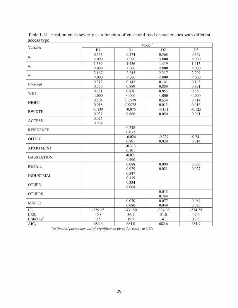
Access Type Models To analyze the logic behind the unexpected negative coefficient on ACCESS, we attempted some microscopic analysis as well. The variable ACCESS was categorized by the number of access points (number of driveways) of different types, including residential, office, retail and industrial. Models were estimated using these categorized variables, with the results summarized in Table I-14. We found that OFFICE is the most significant variable among all access types. Unexpectedly, the variables RETAIL and MINOR in our model increase the crash severity, even though we expect that in retail areas and around the minor intersections, drivers might be more cautious due to more frequent driveway activity and thus drive slower, resulting in the crashes being less severe. Among these driveway types, only OFFICE and RETAIL are significantly correlated with crash severity. Table I-15 shows the number of crashes by severity level for different numbers of retail and office driveways, respectively; these are shown graphically in Figures I-4 and I-5. The range of values for RETAIL is much larger than for OFFICE. When RETAIL is less than 5, the crash severity does have a decreasing tendency along with the increase in the number of RETAIL driveways. However, when RETAIL is larger than 5, the situation is on the contrary. That might cause the final model to produce the mixed results found earlier. These results, along with those reported earlier in the chapter, are summarized and discussed in next section.

- 29 -

Table I-14. Head-on crash severity as a function of crash and road characteristics with different access type

Model* Variable B4 D1 D2 D3

µ1 0.553 <.000

0.574 <.000

0.568 <.000

0.569 <.000

µ2 1.389 <.000

1.436 <.000

1.419 <.000

1.415 <.000

µ3 2.167 <.000

2.245 <.000

2.217 <.000

2.209 <.000

Intercept 0.317 0.750

0.142 0.889

0.141 0.889

0.163 0.871

WET 0.781 <.000

0.836 <.000

0.853 <.000

0.856 <.000

NIGHT 0.504 0.018

0.5779 0.0075

0.534 0.013

0.514 0.016

RWIDTH -0.139 0.037

-0.075 0.668

-0.131 0.050

-0.125 0.061

ACCESS 0.025 0.024

RESIDENCE 0.748 0.072

OFFICE -0.026 0.891

-0.229 0.020

-0.241 0.014

APARTMENT -0.313 0.101

GASSTATION -0.021 0.900

RETAIL 0.088 0.029

0.090 0.021

0.086 0.027

INDUSTRIAL 0.347 0.119

OTHER 0.334 0.068

OTHERS 0.015 0.244

MINOR 0.070 0.080

0.077 0.049

0.084 0.030

LL -339.17 -331.50 -334.06 -334.75 LRS0 Critical χ2

40.8 9.5

56.1 19.7

51.0 14.1

49.6 12.6

AICc 686.6 684.0 682.6 681.9 *estimated parameter and χ2 significance given for each variable

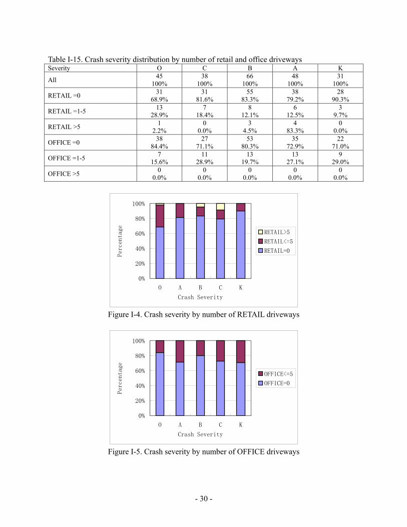
- 30 -

Table I-15. Crash severity distribution by number of retail and office driveways Severity O C B A K

All 45 100%

38 100%

66 100%

48 100%

31 100%

RETAIL =0 31 68.9%

31 81.6%

55 83.3%

38 79.2%

28 90.3%

RETAIL =1-5 13 28.9%

7 18.4%

8 12.1%

6 12.5%

3 9.7%

RETAIL >5 1 2.2%

0 0.0%

3 4.5%

4 83.3%

0 0.0%

OFFICE =0 38 84.4%

27 71.1%

53 80.3%

35 72.9%

22 71.0%

OFFICE =1-5 7 15.6%

11 28.9%

13 19.7%

13 27.1%

9 29.0%

OFFICE >5 0 0.0%

0 0.0%

0 0.0%

0 0.0%

0 0.0%

0%

20%

40%

60%

80%

100%

O A B C K

Crash Severity

Percentage

RETAIL>5

RETAIL<=5

RETAIL=0

Figure I-4. Crash severity by number of RETAIL driveways

0%

20%

40%

60%

80%

100%

O A B C K

Crash Severity

Percentage

OFFICE<=5

OFFICE=0

Figure I-5. Crash severity by number of OFFICE driveways

- 31 -

SUMMARY AND CONCLUSIONS The first phase of this study focused on the roadway geometric features that may explain the incidence of head-on crashes on two-lane rural highways in Connecticut. Negative binomial Generalized Linear Modeling was used for model estimation, and both direct and surrogate geometric variables were investigated for potentially explaining head-on crash risk. Vehicle-kilometers-traveled was used as an offset in the models, taking no multiplicative or exponential parameter. The natural log of AADT was included in all the models to permit the rate of crashes to vary with the traffic volume; the modeling results showed that crash rate decreases slightly with this value. The control variables found alone to have significant effects for predicting head-on crash incidence are speed limit and the sum of the absolute changes in the rate of horizontal curvature (SACRH), the maximum degree of horizontal curve (MAXD), and the sum of the absolute changes in the rate of vertical curvature (SACRV) together in the same model. The model with SACRH performed the best, with the incidence of head-on crashes also increasing with this value. The model with MAXD and SACRV performed nearly as well, with the incidence of head-on crashes also increasing with each. The model with speed limit performed least well, with head-on crashes decreasing as it increases. The second phase of this study is concerned with estimating the severity of head-on crashes as a function of these same types of variables, along with characteristics of the crash itself. Crash data from this same database are being used in the severity study. Ordered Probit modeling is being used to establish the relationship between crash severity and several crash characteristics (e.g., types of vehicles involved, light conditions at the time of the crash), roadway geometric characteristics, and land-use patterns. The severity study extends the findings by discovering which of the same variables are significantly related to head-on crash severity apart from the incidence of crashes, and furthermore to help understand why when a head-on crash occurs, when the crash is likely to be fatal and when it is not. This can help highway safety engineers to implement improvements to two-lane roads aimed not only at reducing the incidence of head-on crashes, but also to ensure that when they do occur that they are less likely to be fatal. Our findings suggest that the best way to reduce the incidence of head-on crashes is to reduce the number of medium to sharp horizontal and vertical curves and to straighten very sharp horizontal curves. This is probably because a greater number of horizontal curves will overtax drivers in following the curving alignment, and a large number of grade changes reduce the sight distance, and thus the ability of drivers to see an oncoming sharp horizontal curve, or oncoming vehicles traveling along the curve. However, road segment horizontal and vertical curvature variables are not promising in head-on crash severity prediction, either as separate factors or as combined factors. One can imagine that when a head-on crash occurs, the drivers may defensively apply the brakes, and try to steer away from the centerline of the road to avoid direct impact. Technically, the severity of a head-on crash will be related to actual impact speed, impact point, the collision angle and the mass of the two involved vehicles. Thus, in that horizontal and vertical curves are likely to affect vehicle speeds, we might expect them to be significant predictors for head-on crash severity. However, in our estimated models, horizontal and vertical curve variables are not significant, even though some

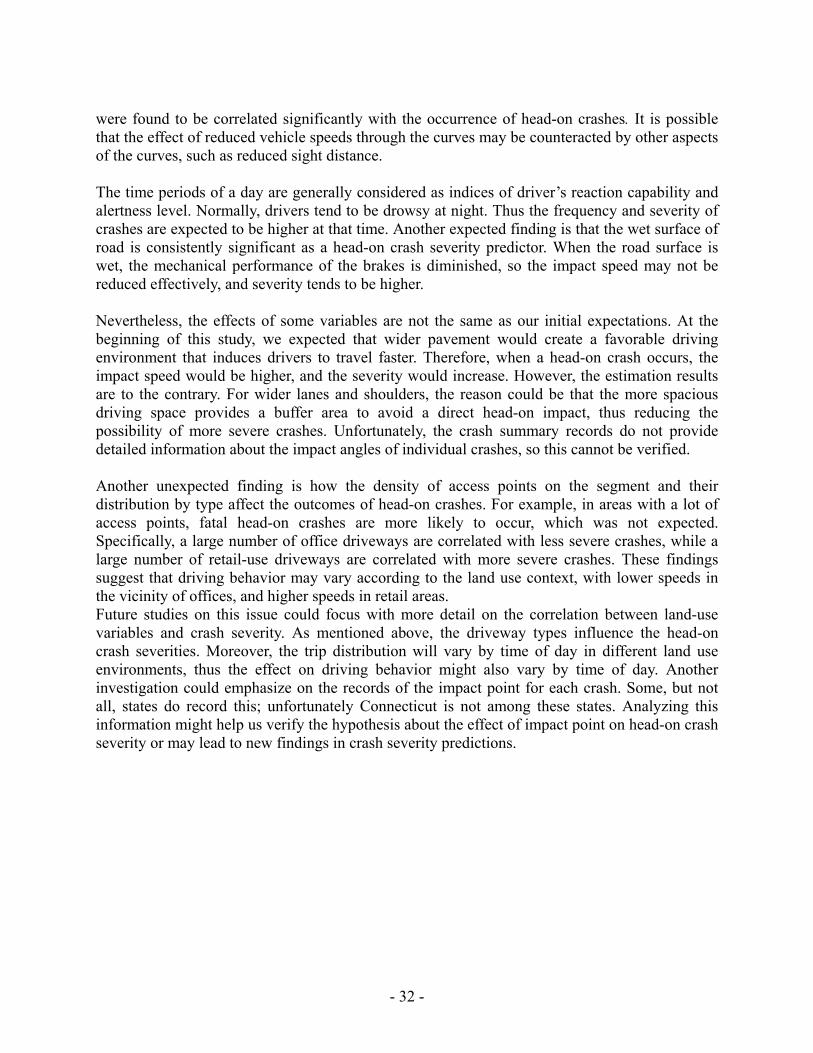
- 32 -

were found to be correlated significantly with the occurrence of head-on crashes. It is possible that the effect of reduced vehicle speeds through the curves may be counteracted by other aspects of the curves, such as reduced sight distance. The time periods of a day are generally considered as indices of driver’s reaction capability and alertness level. Normally, drivers tend to be drowsy at night. Thus the frequency and severity of crashes are expected to be higher at that time. Another expected finding is that the wet surface of road is consistently significant as a head-on crash severity predictor. When the road surface is wet, the mechanical performance of the brakes is diminished, so the impact speed may not be reduced effectively, and severity tends to be higher. Nevertheless, the effects of some variables are not the same as our initial expectations. At the beginning of this study, we expected that wider pavement would create a favorable driving environment that induces drivers to travel faster. Therefore, when a head-on crash occurs, the impact speed would be higher, and the severity would increase. However, the estimation results are to the contrary. For wider lanes and shoulders, the reason could be that the more spacious driving space provides a buffer area to avoid a direct head-on impact, thus reducing the possibility of more severe crashes. Unfortunately, the crash summary records do not provide detailed information about the impact angles of individual crashes, so this cannot be verified. Another unexpected finding is how the density of access points on the segment and their distribution by type affect the outcomes of head-on crashes. For example, in areas with a lot of access points, fatal head-on crashes are more likely to occur, which was not expected. Specifically, a large number of office driveways are correlated with less severe crashes, while a large number of retail-use driveways are correlated with more severe crashes. These findings suggest that driving behavior may vary according to the land use context, with lower speeds in the vicinity of offices, and higher speeds in retail areas. Future studies on this issue could focus with more detail on the correlation between land-use variables and crash severity. As mentioned above, the driveway types influence the head-on crash severities. Moreover, the trip distribution will vary by time of day in different land use environments, thus the effect on driving behavior might also vary by time of day. Another investigation could emphasize on the records of the impact point for each crash. Some, but not all, states do record this; unfortunately Connecticut is not among these states. Analyzing this information might help us verify the hypothesis about the effect of impact point on head-on crash severity or may lead to new findings in crash severity predictions.

- 33 -

REFERENCES

1. Motor Vehicle Traffic Crashes as a Leading Cause of Death in the United States (2002). DOT-HS-809-831. National Center for Statistics and Analysis (NCSA), Washington DC. 2005.

2. Traffic Safety Facts 2003, National Highway Traffic Safety Administration, Washington DC. 2004.

3. Kalakota, K.R., Seneviratne, P.N. and Ossenbruggen, P.J. Influence of Geometric Design Variables on Accident Rates on Two-lane Rural Highways, VTI Report 380A, 1992, pp. 207-226.

4. Qin, X., Ivan J.N. and Ravishanker, N. Selecting exposure measures in crash rate prediction for two-lane highway segments. Accident Analysis & Prevention, Volume 36, No. 2, 2004, pp. 183-191.

5. P Gårder, “Occurrence of Evasive Maneuvers Prior to Accidents-Data from North Carolina Accidents.” Proceedings of the 2nd Workshop of the International Committee on Traffic Conflicts Techniques (ICTCT), Munich, Germany, November 23-24, 1989. Bulletin 86, 13 pages, Lund Institute of Technology, Lund, Sweden, 1990.

6. Coding Manual: Motor Vehicle and Traffic Collision Analysis on Connecticut Streets and Highways, Connecticut Department of Transportation, Newington CT. 1986.

7. Neuman, TR., Pefer, R., Slack, KL., Hardy, KK., McGee, H., Prothe, L., Eccles, K. and Council, F. Guidance for Implementation of the AASHTO Strategic Highway Safety Plan. Volume 4: A Guide for Addressing Head-on Collisions. NCHRP Report 500. 2003.

8. Al-Senan, SH. and Wright PH. Prediction of Head-on Accident Sites. In Transportation Research Record: Journal of the Transportation Research Board, No. 1122, TRB, National Research Council, Washington, D.C., 1987, pp. 79-85.

9. Zegeer, CV., Deen, RC. and Mayes JG. Effect of Lane and Shoulder Widths on Accident Reduction on Rural Two-Lane Roads. In Transportation Research Record: Journal of the Transportation Research Board, No. 806, TRB, National Research Council, Washington, D.C., 1981, pp. 33-43.

10. Leisch, J.E. Traffic Control and Roadway Elements – Their Relationship to Highway Safety – Revised, Chapter 12: Alignment. Highway User Federation for Safety and Mobility. Washington DC. 1971.

11. Agent, K. and Deen, R. Relationship between Roadway Geometrics and Accidents. In Transportation Research Record: Journal of the Transportation Research Board, No. 541, TRB, National Research Council, Washington, D.C., 1975, pp. 1-11.

12. Clissold, CM. Wet Weather Injury Accidents on New Zealand Roads. In Transportation Research Record: Journal of the Transportation Research Board, No. 624, TRB, National Research Council, Washington, D.C., 1976, pp. 136-139.

13. Chira-Chavala, T. and Mak, KK. Identification of Accident Factors on Highway Segments: A Method and Application, In Transportation Research Record: Journal of the Transportation Research Board, No. 1086, TRB, National Research Council, Washington, D.C, 1986. pp. 54-58.

14. Garber, S. and Graham, J. The Effects of the New 65 Mile per Hour Speed Limit on Rural Highway Fatalities: A State-by-State Analysis. Accident Analysis and Prevention, Vol. 22, No. 2, 1990. pp. 137-149.

- 34 -

15. Miaou, S., Hu, P., Wright T., Rathi, A. and Davis, S. Relationship Between Truck Accidents and Highway Geometric Design: A Poisson Regression Approach. In Transportation Research Record: Journal of the Transportation Research Board, No. 1376, TRB, National Research Council, Washington, D.C, 1992. pp. 10-18.

16. Renski, H., Khattak, A. and Council, F. Effect of Speed Limit Increases on Crash Injury Severity: Abalysis of Single-Vehicle Crashes on North Carolina Interstate Highways. In Transportation Research Record: Journal of the Transportation Research Board, No. 1665, TRB, National Research Council, Washington, D.C., 1999, pp. 100-108.

17. Huang, H.; Stewart, J.; Zegeer, C.; 2002. Evaluation of Lane Reduction “Road Diet” Measures on Crashes and Injuries. Transportation Research Record 1784, pp. 70-80.

18. Abdel-Aty, M. Analysis of Driver Injury Severity Levels at Multiple Locations Using Ordered Probit Models, Journal of Safety Research 34. 2003, pp. 597-603

19. Kloeden, C. N., McLean, A. J., Moore, V. M. and Ponte, G. University of Adelaide. NHMRC Road Accident Research Unit. Traveling Speed and the Risk of Crash Involvement., http://casr.adelaide.edu.au/speed. Accessed by July 15, 2005

20. Qin, X and Ivan J.N. Selecting Exposure Measures in Predicting Crash Rates on Two-lane Rural Highways. In Safety, Human Performance. CD-ROM. Transportation Research Board, National Research Council, Washington, D.C., 2002.

21. Traffic Safety Facts 1999, National Highway Traffic Safety Administration, US Department of Transportation, Washington, DC, 2000.

22. Shankar, V., Mannering F., and Barfield, W. Effect of Roadway Geometrics and Environmental Factors on Rural Freeway Accident Frequencies. Accident Analysis and Prevention. Vol. 27, 1995, pp. 371-389.

23. Miaou, S.P, The Relationship between Truck Accidents and Geometric Design of Road Sections: Poisson Versus Negative Binomial Regressions, Accident Analysis and Prevention. Vol. 26, 1994, pp. 471-482.

24. Wang, Y.H, and Nihan N. Estimating the Risk of Collisions between Bicycles and Motor Vehicles at Signalized Intersections. Accident Analysis and Prevention. Vol. 36, 2004, pp. 313-321.

25. Mountain, L., Bachir, F., and Jarrett, D. Accident Prediction Models for Roads With Minor Junctions. Accident Analysis and Prevention. Vol. 28, 1996, pp. 695-707.

26. Hauer, E. Safety and the Choice of Degree of Curve. In Transportation Research Record: Journal of the Transportation Research Board, No. 1665, TRB, National Research Council, Washington, D.C., 1999, pp. 22-27.

27. Neter, J., Kutner, M.H., Nachtsheim, C.J. and Wasserman, W. Applied Linear Statistical Models, Chapter 14, pp567-627 WCB/ McGraw-Hill Press, New York, NY. 1996.

28. Kockelman, KM. and Kweon, Y. Driver Injury Severity: An Application of Ordered Probit Models. Accident Analysis and Prevention, Vol. 33, No. 3, 2002, pp. 313-21.

29. Greene, D.L. and Keller, M. Dissent on Safety Issues: Fuel Economy and Highway Safety, Effectiveness and Impact of Corporate Average Fuel Economy (CAFÉ) Standards. National Academies Press, Washington, DC. 2002.

30. Greene, W.H. Econometric Analysis. Fifth Edition, Prentice Hall, New Jersey. 2003. 31. Sugiura, N. Further analysis of the data by Akaike’s information criterion and the finite

corrections, Communications in Statistics, Theory and Methods A7. 1978, pp. 13-26.

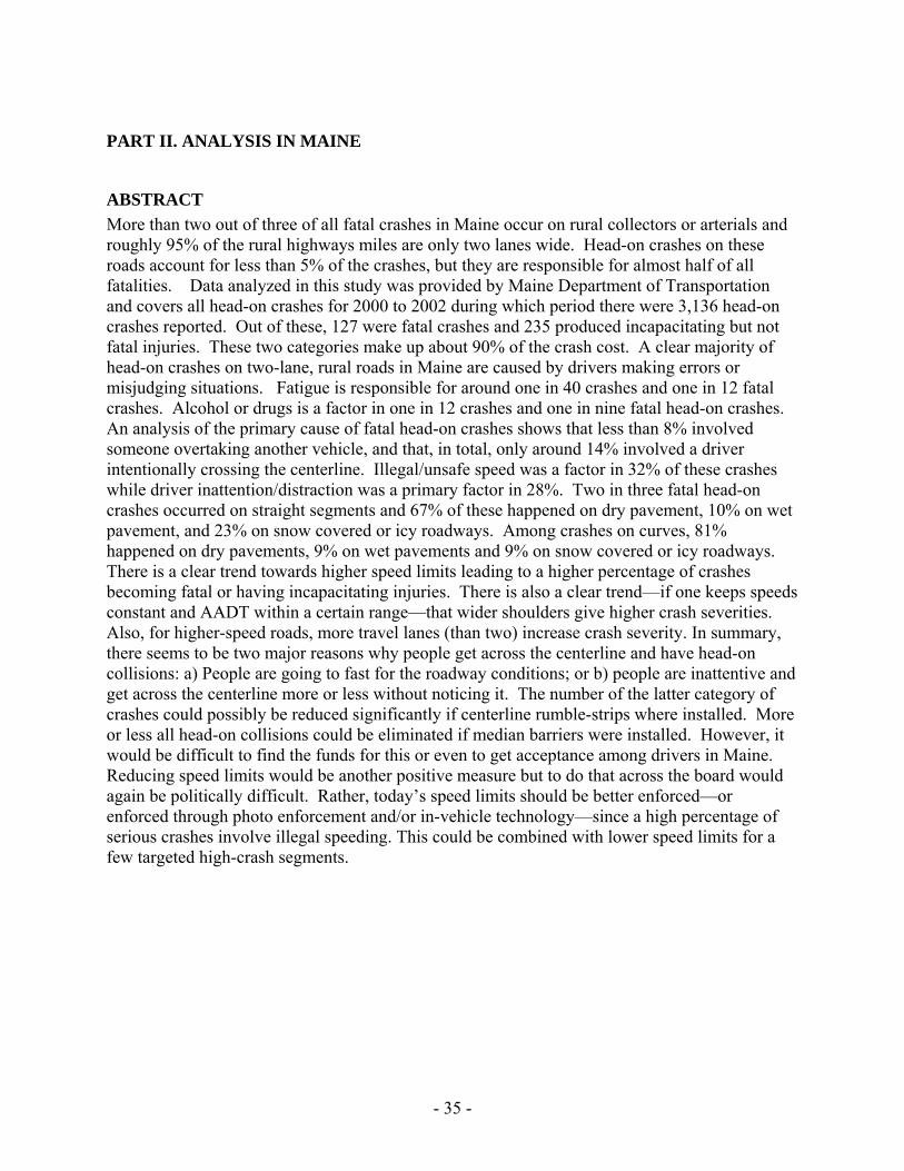
- 35 -

PART II. ANALYSIS IN MAINE

ABSTRACT More than two out of three of all fatal crashes in Maine occur on rural collectors or arterials and roughly 95% of the rural highways miles are only two lanes wide. Head-on crashes on these roads account for less than 5% of the crashes, but they are responsible for almost half of all fatalities. Data analyzed in this study was provided by Maine Department of Transportation and covers all head-on crashes for 2000 to 2002 during which period there were 3,136 head-on crashes reported. Out of these, 127 were fatal crashes and 235 produced incapacitating but not fatal injuries. These two categories make up about 90% of the crash cost. A clear majority of head-on crashes on two-lane, rural roads in Maine are caused by drivers making errors or misjudging situations. Fatigue is responsible for around one in 40 crashes and one in 12 fatal crashes. Alcohol or drugs is a factor in one in 12 crashes and one in nine fatal head-on crashes. An analysis of the primary cause of fatal head-on crashes shows that less than 8% involved someone overtaking another vehicle, and that, in total, only around 14% involved a driver intentionally crossing the centerline. Illegal/unsafe speed was a factor in 32% of these crashes while driver inattention/distraction was a primary factor in 28%. Two in three fatal head-on crashes occurred on straight segments and 67% of these happened on dry pavement, 10% on wet pavement, and 23% on snow covered or icy roadways. Among crashes on curves, 81% happened on dry pavements, 9% on wet pavements and 9% on snow covered or icy roadways. There is a clear trend towards higher speed limits leading to a higher percentage of crashes becoming fatal or having incapacitating injuries. There is also a clear trend—if one keeps speeds constant and AADT within a certain range—that wider shoulders give higher crash severities. Also, for higher-speed roads, more travel lanes (than two) increase crash severity. In summary, there seems to be two major reasons why people get across the centerline and have head-on collisions: a) People are going to fast for the roadway conditions; or b) people are inattentive and get across the centerline more or less without noticing it. The number of the latter category of crashes could possibly be reduced significantly if centerline rumble-strips where installed. More or less all head-on collisions could be eliminated if median barriers were installed. However, it would be difficult to find the funds for this or even to get acceptance among drivers in Maine. Reducing speed limits would be another positive measure but to do that across the board would again be politically difficult. Rather, today’s speed limits should be better enforced—or enforced through photo enforcement and/or in-vehicle technology—since a high percentage of serious crashes involve illegal speeding. This could be combined with lower speed limits for a few targeted high-crash segments.

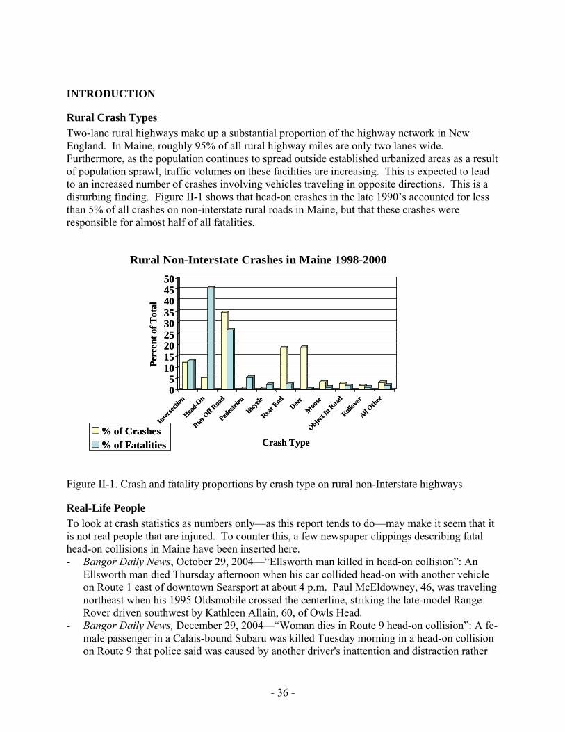
- 36 -

INTRODUCTION

Rural Crash Types Two-lane rural highways make up a substantial proportion of the highway network in New England. In Maine, roughly 95% of all rural highway miles are only two lanes wide. Furthermore, as the population continues to spread outside established urbanized areas as a result of population sprawl, traffic volumes on these facilities are increasing. This is expected to lead to an increased number of crashes involving vehicles traveling in opposite directions. This is a disturbing finding. Figure II-1 shows that head-on crashes in the late 1990’s accounted for less than 5% of all crashes on non-interstate rural roads in Maine, but that these crashes were responsible for almost half of all fatalities.

Figure II-1. Crash and fatality proportions by crash type on rural non-Interstate highways

Real-Life People To look at crash statistics as numbers only—as this report tends to do—may make it seem that it is not real people that are injured. To counter this, a few newspaper clippings describing fatal head-on collisions in Maine have been inserted here. - Bangor Daily News, October 29, 2004—“Ellsworth man killed in head-on collision”: An

Ellsworth man died Thursday afternoon when his car collided head-on with another vehicle on Route 1 east of downtown Searsport at about 4 p.m. Paul McEldowney, 46, was traveling northeast when his 1995 Oldsmobile crossed the centerline, striking the late-model Range Rover driven southwest by Kathleen Allain, 60, of Owls Head.

- Bangor Daily News, December 29, 2004—“Woman dies in Route 9 head-on collision”: A fe-male passenger in a Calais-bound Subaru was killed Tuesday morning in a head-on collision on Route 9 that police said was caused by another driver's inattention and distraction rather

Rural Non-Interstate Crashes in Maine 1998-2000

05

101520253035404550

Perc

ent o

f Tot

al

Inter

sectio

n

Head-O

n

Run Off R

oad

Pedest

rian

Bicycle

Rear End

Deer

Moo

se

Object I

n Road

Rollov

er

All Other

Crash Type% of Crashes% of Fatalities

05

101520253035404550

Perc

ent o

f Tot

al

Inter

sectio

n

Head-O

n

Run Off R

oad

Pedest

rian

Bicycle

Rear End

Deer

Moo

se

Object I

n Road

Rollov

er

All Other

Crash Type% of Crashes% of Fatalities

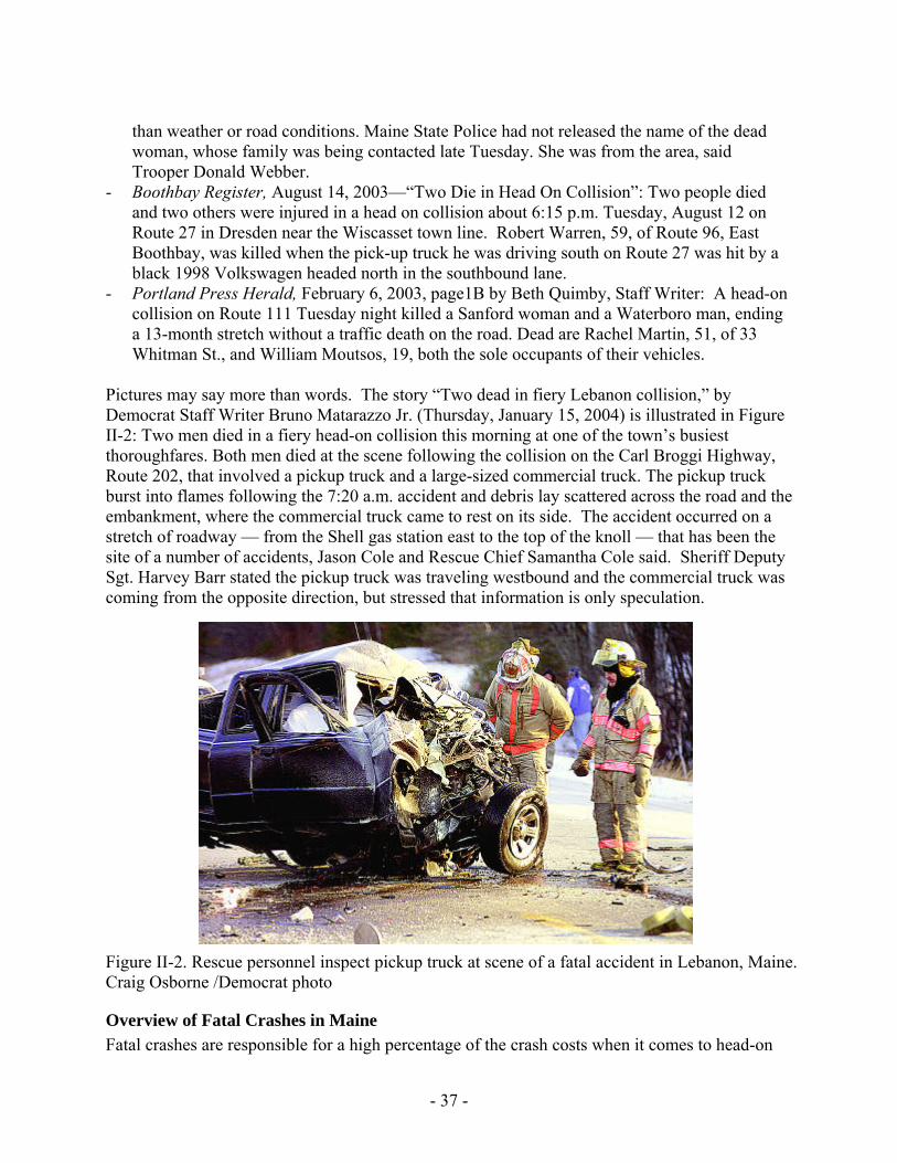
- 37 -

than weather or road conditions. Maine State Police had not released the name of the dead woman, whose family was being contacted late Tuesday. She was from the area, said Trooper Donald Webber.

- Boothbay Register, August 14, 2003—“Two Die in Head On Collision”: Two people died and two others were injured in a head on collision about 6:15 p.m. Tuesday, August 12 on Route 27 in Dresden near the Wiscasset town line. Robert Warren, 59, of Route 96, East Boothbay, was killed when the pick-up truck he was driving south on Route 27 was hit by a black 1998 Volkswagen headed north in the southbound lane.

- Portland Press Herald, February 6, 2003, page1B by Beth Quimby, Staff Writer: A head-on collision on Route 111 Tuesday night killed a Sanford woman and a Waterboro man, ending a 13-month stretch without a traffic death on the road. Dead are Rachel Martin, 51, of 33 Whitman St., and William Moutsos, 19, both the sole occupants of their vehicles.

Pictures may say more than words. The story “Two dead in fiery Lebanon collision,” by Democrat Staff Writer Bruno Matarazzo Jr. (Thursday, January 15, 2004) is illustrated in Figure II-2: Two men died in a fiery head-on collision this morning at one of the town’s busiest thoroughfares. Both men died at the scene following the collision on the Carl Broggi Highway, Route 202, that involved a pickup truck and a large-sized commercial truck. The pickup truck burst into flames following the 7:20 a.m. accident and debris lay scattered across the road and the embankment, where the commercial truck came to rest on its side. The accident occurred on a stretch of roadway — from the Shell gas station east to the top of the knoll — that has been the site of a number of accidents, Jason Cole and Rescue Chief Samantha Cole said. Sheriff Deputy Sgt. Harvey Barr stated the pickup truck was traveling westbound and the commercial truck was coming from the opposite direction, but stressed that information is only speculation.

Figure II-2. Rescue personnel inspect pickup truck at scene of a fatal accident in Lebanon, Maine. Craig Osborne /Democrat photo

Overview of Fatal Crashes in Maine Fatal crashes are responsible for a high percentage of the crash costs when it comes to head-on

- 38 -

collisions. (As shown on page 40, over 75% of the total crash cost of head-on collisions in Maine is attributed to fatal crashes.) Also, fatal crashes are reported to a higher degree than any other type, are the ones that are the most thoroughly investigated with respect to cause, and are the ones that easiest can be found in data banks. An overview of fatal crashes will therefore be provided already here in the introductory section. Fatal as well as non-fatal head-on crashes are analyzed in detail in the results section starting on page 40. Rural, non-interstate crashes, the ones presented in Figure II-1, make up a clear majority of the fatal crashes in the state of Maine. The Fatality Analysis Reporting System (FARS) Web-Based Encyclopedia shows that there in 2002 were 186 fatal crashes in Maine involving 272 vehicles. Fourteen (8%) of the fatal crashes occurred on rural interstate highways, 58 (31%) on other rural arterials, 55 (30%) on rural collector roads, 38 (20%) on rural local roads, and 4 on rural roads with unknown classification. There were two crashes with unknown urban/rural designation. This means that over 90% (169 to 171 out of 186) of the fatal crashes in the state were rural and less than 10% (15 to 17) occurred in urban areas. The fact that more than two out of three (127 to 133 out of 186) of all fatal crashes in Maine occurred on rural collectors/arterials means that this is where a considerable part of the safety improvement efforts ought to be concentrated. And, head-on collisions are the ones taking roughly half of all lives on these roads.

Possible Causation of Head-On Collisions Clearly, something should be done to reduce the number of head-on collisions on rural collector roads and arterials. An obvious first step is to identify what is causing these head-on crashes—especially the fatal ones—and do whatever is necessary to reduce their occurrence, or at least their severity. Obviously, in order for a head-on crash to occur, one vehicle must cross the centerline of the road. The reasons drivers cross the centerline can be divided into intentional and unintentional ones. Examples of intentional reasons are: ● overtaking slower vehicles ● turning left ● making shortcuts through left-hand curves ● intent to commit suicide1 Examples of unintentional crossovers are: ● inattentiveness, distraction ● having fallen asleep ● inability to see centerline, e.g. when roadway is covered by snow ● losing control because of speeding, especially in right-hand curves ● over-correction after running off the right edge of the pavement

1 These events are not accidents and therefore typically not included in accident or crash statistics. However, they

clearly are collisions (and crashes) and a Norwegian study show that in that country close to half of all fatal head-on collisions involving heavy trucks seem to be suicides.

- 39 -

DATA The primary data analyzed in this study was provided by Maine Department of Transportation. The material includes computer files listing all the state’s head-on crashes for 2000 to 2002. These files integrate characteristics of each crash and the roadway on which it happened, including: the jurisdiction, town name, route name, street name, estimated mile point, link node identification, segment identification, crash date, hour of day, day of week, weather condition, road surface condition, light condition, number of fatalities, number of incapacitating injuries, number of evident injuries, number of possible injuries, estimated economic impact, factored AADT, federal functional class jurisdiction, speed limit (mph), average median width (ft), shoulder width left (ft), shoulder type left, shoulder width right (ft), shoulder type right, number of lanes, apparent contributing crash factors, driver ages, driver physical conditions, pre-crash actions, vehicle types, and driver license types. Another file compiled from the previous ones lists the number of crashes on each one-mile segment2 of the State highways and State-aid roads. A third file gives essential characteristics of these one-mile segments. Data provided by FARS has also been used in this study.

2 The roads were all divided into one-mile segments. However, the ‘end’ segment is almost always shorter since a

route typically doesn’t have a length of even miles.

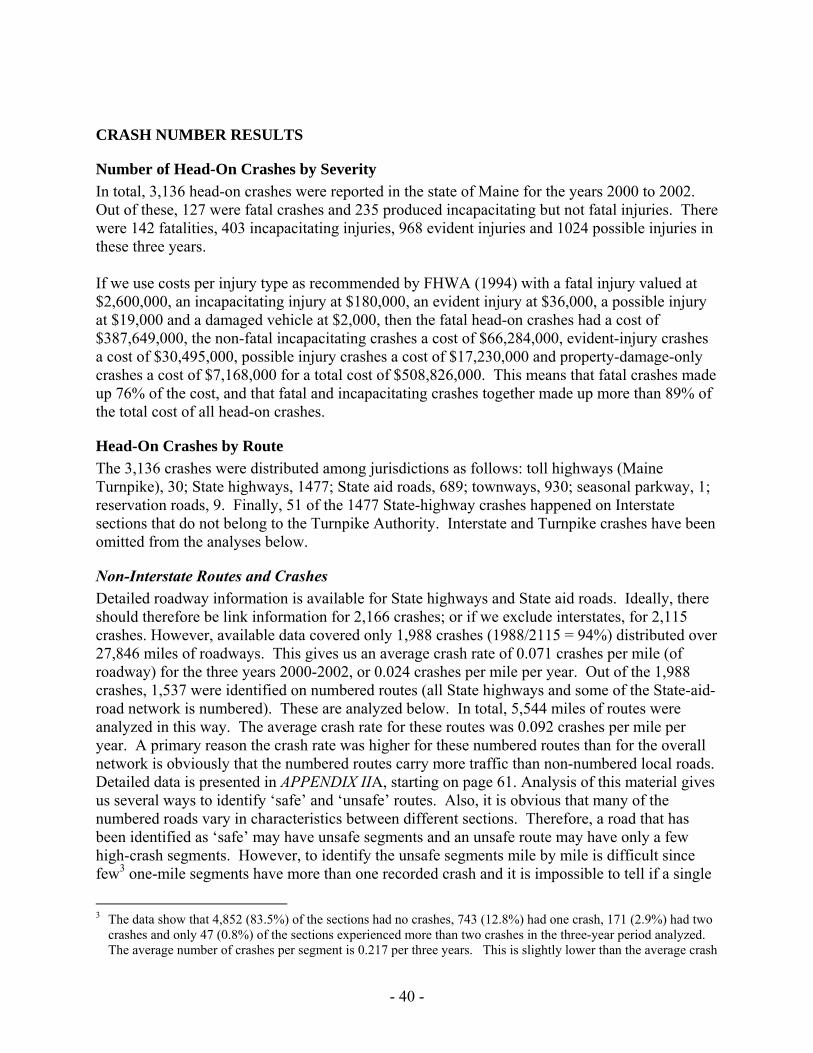
- 40 -

CRASH NUMBER RESULTS

Number of Head-On Crashes by Severity In total, 3,136 head-on crashes were reported in the state of Maine for the years 2000 to 2002. Out of these, 127 were fatal crashes and 235 produced incapacitating but not fatal injuries. There were 142 fatalities, 403 incapacitating injuries, 968 evident injuries and 1024 possible injuries in these three years. If we use costs per injury type as recommended by FHWA (1994) with a fatal injury valued at $2,600,000, an incapacitating injury at $180,000, an evident injury at $36,000, a possible injury at $19,000 and a damaged vehicle at $2,000, then the fatal head-on crashes had a cost of $387,649,000, the non-fatal incapacitating crashes a cost of $66,284,000, evident-injury crashes a cost of $30,495,000, possible injury crashes a cost of $17,230,000 and property-damage-only crashes a cost of $7,168,000 for a total cost of $508,826,000. This means that fatal crashes made up 76% of the cost, and that fatal and incapacitating crashes together made up more than 89% of the total cost of all head-on crashes.

Head-On Crashes by Route The 3,136 crashes were distributed among jurisdictions as follows: toll highways (Maine Turnpike), 30; State highways, 1477; State aid roads, 689; townways, 930; seasonal parkway, 1; reservation roads, 9. Finally, 51 of the 1477 State-highway crashes happened on Interstate sections that do not belong to the Turnpike Authority. Interstate and Turnpike crashes have been omitted from the analyses below.

Non-Interstate Routes and Crashes Detailed roadway information is available for State highways and State aid roads. Ideally, there should therefore be link information for 2,166 crashes; or if we exclude interstates, for 2,115 crashes. However, available data covered only 1,988 crashes (1988/2115 = 94%) distributed over 27,846 miles of roadways. This gives us an average crash rate of 0.071 crashes per mile (of roadway) for the three years 2000-2002, or 0.024 crashes per mile per year. Out of the 1,988 crashes, 1,537 were identified on numbered routes (all State highways and some of the State-aid-road network is numbered). These are analyzed below. In total, 5,544 miles of routes were analyzed in this way. The average crash rate for these routes was 0.092 crashes per mile per year. A primary reason the crash rate was higher for these numbered routes than for the overall network is obviously that the numbered routes carry more traffic than non-numbered local roads. Detailed data is presented in APPENDIX IIA, starting on page 61. Analysis of this material gives us several ways to identify ‘safe’ and ‘unsafe’ routes. Also, it is obvious that many of the numbered roads vary in characteristics between different sections. Therefore, a road that has been identified as ‘safe’ may have unsafe segments and an unsafe route may have only a few high-crash segments. However, to identify the unsafe segments mile by mile is difficult since few3 one-mile segments have more than one recorded crash and it is impossible to tell if a single

3 The data show that 4,852 (83.5%) of the sections had no crashes, 743 (12.8%) had one crash, 171 (2.9%) had two

crashes and only 47 (0.8%) of the sections experienced more than two crashes in the three-year period analyzed. The average number of crashes per segment is 0.217 per three years. This is slightly lower than the average crash

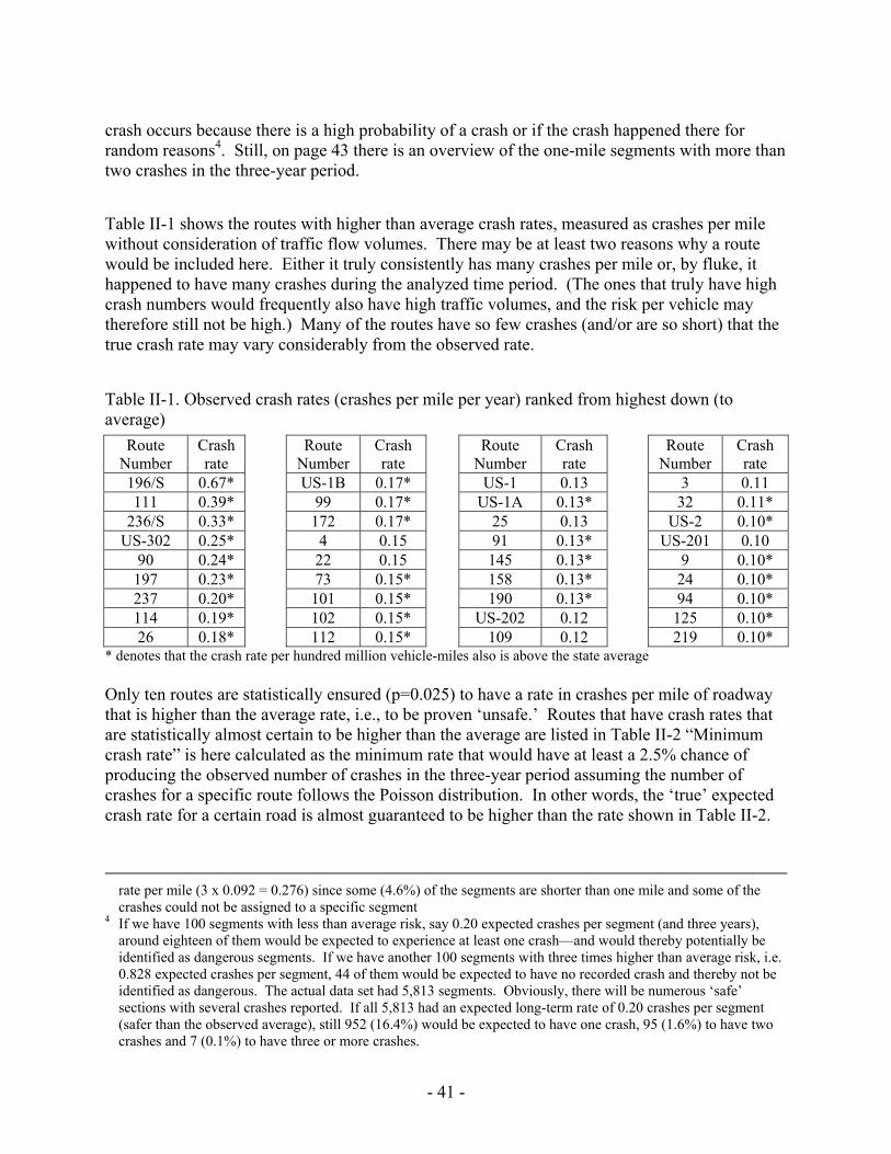
- 41 -

crash occurs because there is a high probability of a crash or if the crash happened there for random reasons4. Still, on page 43 there is an overview of the one-mile segments with more than two crashes in the three-year period. Table II-1 shows the routes with higher than average crash rates, measured as crashes per mile without consideration of traffic flow volumes. There may be at least two reasons why a route would be included here. Either it truly consistently has many crashes per mile or, by fluke, it happened to have many crashes during the analyzed time period. (The ones that truly have high crash numbers would frequently also have high traffic volumes, and the risk per vehicle may therefore still not be high.) Many of the routes have so few crashes (and/or are so short) that the true crash rate may vary considerably from the observed rate. Table II-1. Observed crash rates (crashes per mile per year) ranked from highest down (to average)

Route Number

Crash rate

Route Number

Crash rate

Route Number

Crash rate

Route Number

Crash rate

196/S 0.67* US-1B 0.17* US-1 0.13 3 0.11 111 0.39* 99 0.17* US-1A 0.13* 32 0.11*

236/S 0.33* 172 0.17* 25 0.13 US-2 0.10* US-302 0.25* 4 0.15 91 0.13* US-201 0.10

90 0.24* 22 0.15 145 0.13* 9 0.10* 197 0.23* 73 0.15* 158 0.13* 24 0.10* 237 0.20* 101 0.15* 190 0.13* 94 0.10* 114 0.19* 102 0.15* US-202 0.12 125 0.10* 26 0.18* 112 0.15* 109 0.12 219 0.10*

* denotes that the crash rate per hundred million vehicle-miles also is above the state average Only ten routes are statistically ensured (p=0.025) to have a rate in crashes per mile of roadway that is higher than the average rate, i.e., to be proven ‘unsafe.’ Routes that have crash rates that are statistically almost certain to be higher than the average are listed in Table II-2 “Minimum crash rate” is here calculated as the minimum rate that would have at least a 2.5% chance of producing the observed number of crashes in the three-year period assuming the number of crashes for a specific route follows the Poisson distribution. In other words, the ‘true’ expected crash rate for a certain road is almost guaranteed to be higher than the rate shown in Table II-2.

rate per mile (3 x 0.092 = 0.276) since some (4.6%) of the segments are shorter than one mile and some of the crashes could not be assigned to a specific segment

4 If we have 100 segments with less than average risk, say 0.20 expected crashes per segment (and three years), around eighteen of them would be expected to experience at least one crash—and would thereby potentially be identified as dangerous segments. If we have another 100 segments with three times higher than average risk, i.e. 0.828 expected crashes per segment, 44 of them would be expected to have no recorded crash and thereby not be identified as dangerous. The actual data set had 5,813 segments. Obviously, there will be numerous ‘safe’ sections with several crashes reported. If all 5,813 had an expected long-term rate of 0.20 crashes per segment (safer than the observed average), still 952 (16.4%) would be expected to have one crash, 95 (1.6%) to have two crashes and 7 (0.1%) to have three or more crashes.

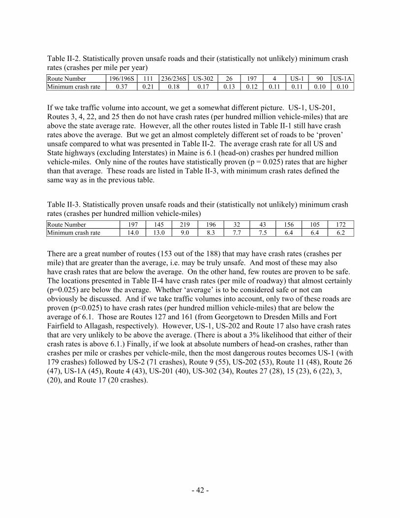
- 42 -

Table II-2. Statistically proven unsafe roads and their (statistically not unlikely) minimum crash rates (crashes per mile per year) Route Number 196/196S 111 236/236S US-302 26 197 4 US-1 90 US-1AMinimum crash rate 0.37 0.21 0.18 0.17 0.13 0.12 0.11 0.11 0.10 0.10

If we take traffic volume into account, we get a somewhat different picture. US-1, US-201, Routes 3, 4, 22, and 25 then do not have crash rates (per hundred million vehicle-miles) that are above the state average rate. However, all the other routes listed in Table II-1 still have crash rates above the average. But we get an almost completely different set of roads to be ‘proven’ unsafe compared to what was presented in Table II-2. The average crash rate for all US and State highways (excluding Interstates) in Maine is 6.1 (head-on) crashes per hundred million vehicle-miles. Only nine of the routes have statistically proven (p = 0.025) rates that are higher than that average. These roads are listed in Table II-3, with minimum crash rates defined the same way as in the previous table. Table II-3. Statistically proven unsafe roads and their (statistically not unlikely) minimum crash rates (crashes per hundred million vehicle-miles) Route Number 197 145 219 196 32 43 156 105 172 Minimum crash rate 14.0 13.0 9.0 8.3 7.7 7.5 6.4 6.4 6.2

There are a great number of routes (153 out of the 188) that may have crash rates (crashes per mile) that are greater than the average, i.e. may be truly unsafe. And most of these may also have crash rates that are below the average. On the other hand, few routes are proven to be safe. The locations presented in Table II-4 have crash rates (per mile of roadway) that almost certainly (p=0.025) are below the average. Whether ‘average’ is to be considered safe or not can obviously be discussed. And if we take traffic volumes into account, only two of these roads are proven (p<0.025) to have crash rates (per hundred million vehicle-miles) that are below the average of 6.1. Those are Routes 127 and 161 (from Georgetown to Dresden Mills and Fort Fairfield to Allagash, respectively). However, US-1, US-202 and Route 17 also have crash rates that are very unlikely to be above the average. (There is about a 3% likelihood that either of their crash rates is above 6.1.) Finally, if we look at absolute numbers of head-on crashes, rather than crashes per mile or crashes per vehicle-mile, then the most dangerous routes becomes US-1 (with 179 crashes) followed by US-2 (71 crashes), Route 9 (55), US-202 (53), Route 11 (48), Route 26 (47), US-1A (45), Route 4 (43), US-201 (40), US-302 (34), Routes 27 (28), 15 (23), 6 (22), 3, (20), and Route 17 (20 crashes).

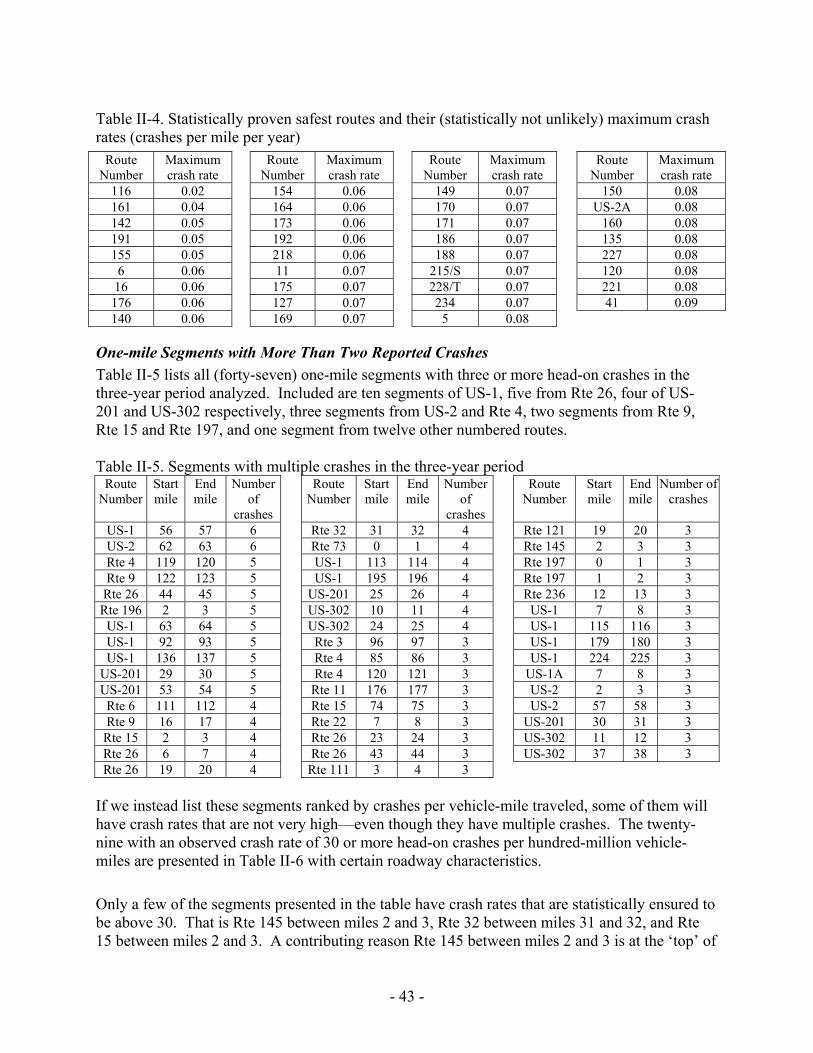
- 43 -

Table II-4. Statistically proven safest routes and their (statistically not unlikely) maximum crash rates (crashes per mile per year)

Route Number

Maximum crash rate

Route Number

Maximum crash rate

Route Number

Maximum crash rate

Route Number

Maximum crash rate

116 0.02 154 0.06 149 0.07 150 0.08 161 0.04 164 0.06 170 0.07 US-2A 0.08 142 0.05 173 0.06 171 0.07 160 0.08 191 0.05 192 0.06 186 0.07 135 0.08 155 0.05 218 0.06 188 0.07 227 0.08 6 0.06 11 0.07 215/S 0.07 120 0.08

16 0.06 175 0.07 228/T 0.07 221 0.08 176 0.06 127 0.07 234 0.07 41 0.09 140 0.06 169 0.07 5 0.08

One-mile Segments with More Than Two Reported Crashes Table II-5 lists all (forty-seven) one-mile segments with three or more head-on crashes in the three-year period analyzed. Included are ten segments of US-1, five from Rte 26, four of US-201 and US-302 respectively, three segments from US-2 and Rte 4, two segments from Rte 9, Rte 15 and Rte 197, and one segment from twelve other numbered routes. Table II-5. Segments with multiple crashes in the three-year period

Route Number

Start mile

End mile

Number of

crashes

Route Number

Start mile

End mile

Number of

crashes

Route Number

Start mile

End mile

Number of crashes

US-1 56 57 6 Rte 32 31 32 4 Rte 121 19 20 3 US-2 62 63 6 Rte 73 0 1 4 Rte 145 2 3 3 Rte 4 119 120 5 US-1 113 114 4 Rte 197 0 1 3 Rte 9 122 123 5 US-1 195 196 4 Rte 197 1 2 3

Rte 26 44 45 5 US-201 25 26 4 Rte 236 12 13 3 Rte 196 2 3 5 US-302 10 11 4 US-1 7 8 3

US-1 63 64 5 US-302 24 25 4 US-1 115 116 3 US-1 92 93 5 Rte 3 96 97 3 US-1 179 180 3 US-1 136 137 5 Rte 4 85 86 3 US-1 224 225 3

US-201 29 30 5 Rte 4 120 121 3 US-1A 7 8 3 US-201 53 54 5 Rte 11 176 177 3 US-2 2 3 3 Rte 6 111 112 4 Rte 15 74 75 3 US-2 57 58 3 Rte 9 16 17 4 Rte 22 7 8 3 US-201 30 31 3

Rte 15 2 3 4 Rte 26 23 24 3 US-302 11 12 3 Rte 26 6 7 4 Rte 26 43 44 3 US-302 37 38 3 Rte 26 19 20 4 Rte 111 3 4 3

If we instead list these segments ranked by crashes per vehicle-mile traveled, some of them will have crash rates that are not very high—even though they have multiple crashes. The twenty-nine with an observed crash rate of 30 or more head-on crashes per hundred-million vehicle-miles are presented in Table II-6 with certain roadway characteristics. Only a few of the segments presented in the table have crash rates that are statistically ensured to be above 30. That is Rte 145 between miles 2 and 3, Rte 32 between miles 31 and 32, and Rte 15 between miles 2 and 3. A contributing reason Rte 145 between miles 2 and 3 is at the ‘top’ of

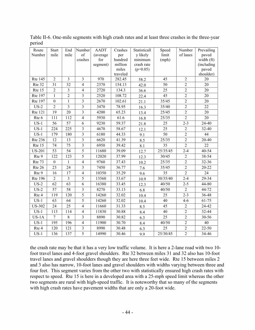
- 44 -

Table II-6. One-mile segments with high crash rates and at least three crashes in the three-year period

Route Number

Start mile

End mile

Number of

crashes

AADT (average

for segment)

Crashes per

hundred million miles

traveled

Statistically likely

minimum crash rate (p=0.05)

Speed limit

(mph)

Number of lanes

Prevailing paved

width (ft) (including

paved shoulder)

Rte 145 2 3 3 970 282.45 58.2 45 2 20 Rte 32 31 32 4 2370 154.13 42.0 50 2 20 Rte 15 2 3 4 2720 134.3 36.6 25 2 20

Rte 197 1 2 3 2520 108.72 22.4 45 2 20 Rte 197 0 1 3 2670 102.61 21.1 35/45 2 20

US-2 2 3 3 3470 78.95 16.3 35/40 2 22 Rte 121 19 20 3 4200 65.23 13.4 25/45 2 20

Rte 6 111 112 4 5930 61.6 16.8 25/35 2 20 US-1 56 57 6 9230 59.37 21.8 25 2-3 24-40 US-1 224 225 3 4670 58.67 12.1 25 2 32-40 US-1 179 180 3 6180 44.33 9.1 50 2 44

Rte 236 12 13 3 6620 41.39 8.5 25/35 2 20-40 Rte 15 74 75 3 6950 39.42 8.1 35 2 22 US-201 53 54 5 11680 39.09 12.7 25/35/45 2-4 40-54 Rte 9 122 123 5 12020 37.99 12.3 30/45 2 38-54

Rte 73 0 1 4 9760 37.43 10.2 25/35 2 32-36 Rte 26 23 24 3 7450 36.77 7.6 35/45 2 20-22 Rte 9 16 17 4 10350 35.29 9.6 35 2 24

Rte 196 2 3 5 13560 33.67 10.9 30/35/40 2-4 29-34 US-2 62 63 6 16380 33.45 12.3 40/50 2-5 44-80 US-2 57 58 3 8270 33.13 6.8 40/50 2 44-72 Rte 4 119 120 5 14260 32.02 10.4 25 2-3 36-48 US-1 63 64 5 14260 32.02 10.4 40 4-6 61-75

US-302 24 25 4 11660 31.33 8.5 45 2 24-42 US-1 113 114 4 11830 30.88 8.4 40 2 32-44

US-1A 7 8 3 8890 30.82 6.3 25 2 30-56 US-1 195 196 4 11900 30.70 8.4 40/50 2 40 Rte 4 120 121 3 8990 30.48 6.3 25 2 22-50 US-1 136 137 5 14990 30.46 9.9 25/30/45 2 34-46

the crash rate may be that it has a very low traffic volume. It is here a 2-lane road with two 10-foot travel lanes and 4-foot gravel shoulders. Rte 32 between miles 31 and 32 also has 10-foot travel lanes and gravel shoulders though they are here three feet wide. Rte 15 between miles 2 and 3 also has narrow, 10-foot lanes and gravel shoulders with widths varying between three and four feet. This segment varies from the other two with statistically ensured high crash rates with respect to speed. Rte 15 is here in a developed area with a 25-mph speed limit whereas the other two segments are rural with high-speed traffic. It is noteworthy that so many of the segments with high crash rates have pavement widths that are only a 20-foot wide.

- 45 -

Fatal Crashes As mentioned above, there were 127 fatal head-on crashes in the state and 104 of those occurred on non-Interstate State highways or State aid roads. By absolute numbers, the most crash prone route was US-1 with 18 fatal crashes followed by US-2 with eight, and US-202 with six. Then follows Routes 4 and 111 with five fatal crashes each, Routes 9 and 11 with four each, and US-1A, US-201, Routes 3 and 26 with three each. Measured as fatal crashes per mile of roadway, 37 out of the 188 routes have observed crash rates that are higher than the average of 0.0060 fatal crashes per mile per year. The worst were Rte 111 (with a rate of 0.139), Rte 207 (0.083), Rte 196/196S (0.048), and Rte 99 (0.042 fatal crashes per mile). US-1, US-1A, US-2, US-2A, US-201, US-202 and US-302 all have rates between 0.007 and 0.016 fatal crashes per mile of roadway. Only two routes are statistically significantly (p=0.025) proven to have more crashes per mile than the average road. That is Route 111 (which goes between Alfred and Biddeford) and US-1. However, 134 of the 188 routes may statistically (p=0.025) be more dangerous than the average road. There is not a single route that is statistically ensured (p=0.025) to have a fatality rate below 0.0060 crashes per mile, meaning that there is no route that is ‘proven’ to be safer than the average road. The route that is closest to being proven safer is Route 16 (which goes from the New Hampshire border to Orono), followed by Routes 11 and 17. If we take traffic volumes into account, the average crash rate becomes 0.504 fatal (head-on) crashes per hundred million vehicle-miles. Only Route 111 (which goes between Alfred and Biddeford) has a fatality rate that is significantly ensured (p<0.025) to be above that, meaning it is almost definitely a high-risk route with respect to fatalities. There is not a single route that is statistically ensured to have a fatality rate below 0.504 crashes per hundred million vehicle-miles, meaning that there is no route that is ‘proven’ to be safer than average. The route that is closest to being proven safer is Route 17 (which stretches from Rockland to Rangeley).

Fatality Share Out of the routes that had at least ten reported head-on crashes in the three-year period, the share that was fatal has been calculated. The highest share was found for Route 111 with 5 out of 14 crashes being fatal. That is followed by Route 139 (2 out of 10), Route 24 (2 out of 11), Route 3 (3 out of 20), Route 4 (5 out of 43), US-202 (6 out of 53), US-2 (8 out of 71), Route 32 (2 out of 18), and US-1 (18 out of 179). The average fatality share for all analyzed routes was 8.2%. Only Route 111 has a share which is statistically significantly greater than the average (p<0.025).

Cause of Crashes Below follows a detailed analysis of causes behind fatal crashes as construed from the crash reports. One reason only fatal crashes are analyzed in detail is that these are the ones with the most reliable data. Another reason is that an analysis of a small number of crashes illuminates the causation of roughly three quarters of the crash cost. The association between design characteristics and non-fatal crash numbers is discussed on page 49.

- 46 -

Fatal Crashes The primary cause was analyzed for the 127 fatal head-on crashes that occurred in the state in 2000-2002. Three of them, occurring on Interstate facilities, are excluded from further analysis5. Based on the police reports, the primary cause of the remaining 124 crashes has been assessed by the author of this report as outlined below. It should be noted that it is the primary cause of the crash, not the primary cause of the fatality that is listed. For example, a crash would be listed as sleep related when a driver crosses the center line after falling asleep even if it may be high speed of the oncoming vehicle that made the crash fatal. On the other hand, if a speeding driver crosses the center line and collides with a drunk driver who is driving properly; that crash would be listed as speed related and not as alcohol related6. Known suicides—if any—are not included in the statistics provided by Maine DOT. There are a few crashes that are very clearly attributed to driver error, e.g. eight cases were caused by a driver having fallen asleep. These are easy to categorize and there is one vehicle defect, defective tire - tire failure, which is equally easy to classify, but many crashes are difficult to attribute to only one factor. Therefore, multiple causes are sometimes listed. Intentional Crossovers: A majority of the crashes listed under this subheading would be intentional. Certainly, people typically must cross the centerline when passing slower vehicles on a two-lane road but all lane changes may not necessarily be intentional crossovers. ● overtaking vehicles, while sober: 7 crashes ● overtaking vehicles, while under the influence of alcohol/drinking: 3 crashes ● turning left, while under the influence of alcohol/drinking: 1 crash ● avoiding vehicle changing lanes, while under the influence of alcohol/drinking: 1 crash ● driving left of center, not passing, while avoiding someone changing lanes: 3 crashes ● driving left of center, not passing, while avoiding someone slowing: 1 crash ● driving left of center, not passing, while avoiding vehicle, object, ped, or animal in road: 2 cr. In total, there were 18 crashes that most likely were caused by an intentional crossover (across the centerline). A few of these may have been ‘necessary’ to avoid rear-ending another vehicle or hitting a pedestrian but most of those probably had improved mobility as primary objective. Possibly Intentional Crossovers: The crashes listed in this subgroup cannot easily be classified into intentional versus unintentional crossovers. For example, a person being under the influence of alcohol—as well as a sober person—may be making intentional shortcuts through left-hand curves. But, probably, only a small fraction of the crashes listed here should be considered intentional. ● driving left of center, not passing, while under the influence of alcohol/drinking: 12 crashes ● driving left of center, not passing, while using drugs: 2 crashes

5 Two of those happened on the Turnpike—in Scarborough and Auburn respectively—where drivers in both cases

drove the wrong way into opposing traffic, one of these drivers was under the influence of alcohol. The third crash happened on the Interstate in Falmouth where an 84-year old handicapped driver made a left turn.

6 An actual case involved a driver under the influence of alcohol colliding with another driver under the influence of drugs. The latter was driving on the wrong side of the road.

- 47 -

● driving left of center, not passing, while illegally speeding: 9 crashes ● driving left of center, not passing, while sober, awake and not distracted, etc: 18 crashes In total, there were 41 crashes that probably were caused by unintentional crossover of the centerline but where intention cannot be ruled out. Unintentional Crossovers: A small percentage of the crashes listed below may also be intentional but the chances that these are intentional are assessed by the author as very small. This does not mean that a different behavior by the driver would not have eliminated the crash from happening. ● driving left of center, not passing, while inattentive/distracted: 16 crashes ● driving left of center, not passing, or wrong way after having fallen asleep/fatigued: 11 crashes ● skidding across, while under the influence of alcohol/drinking: 2 crashes ● skidding across, while ill: 1 crash ● skidding across, while snow and illegal speed and sober: 13 crashes ● skidding across, while snow but not illegal speed: 6 crashes ● skidding across when dry road; illegal speed: 8 crashes ● skidding across after tire failure, 1 crash ● skidding across when dry road; no other apparent factor: 7 crashes In total, there were 65 crashes that almost certainly were caused by an unintentional crossover (across the centerline). In the listings above, only the most important reasons for a crash were included. In some instances, there were also secondary or tertiary causes (contributing factors, physical conditions and pre-crash actions) indicated in the police report. In total, 271 drivers were involved in the 124 fatal crashes analyzed. Table II-7 shows 436 alphabetically ordered apparent contributing factors (a maximum of two per driver), physical conditions, and pre-crash actions as they were reported—for a maximum of four factors per driver. These factors are also summarized in Table II-8 into categories showing whether a specific crash was caused primarily by driver error, vehicle factors or roadway/environmental factors. The added up numbers of the two tables differ somewhat because factors which do not add any real information such as ‘other,’ ‘unknown,’ and “driving left of center without passing other vehicle” were excluded from the latter table. In summary, it can be concluded that human factors are the most common causes of head-on crashes. However, roadway characteristics and vehicle design can certainly influence the outcome of a crash as well as the likelihood that there will be a crash since both the risk of making a human error and the risk that making that error will lead to a collision can be influenced by external factors.

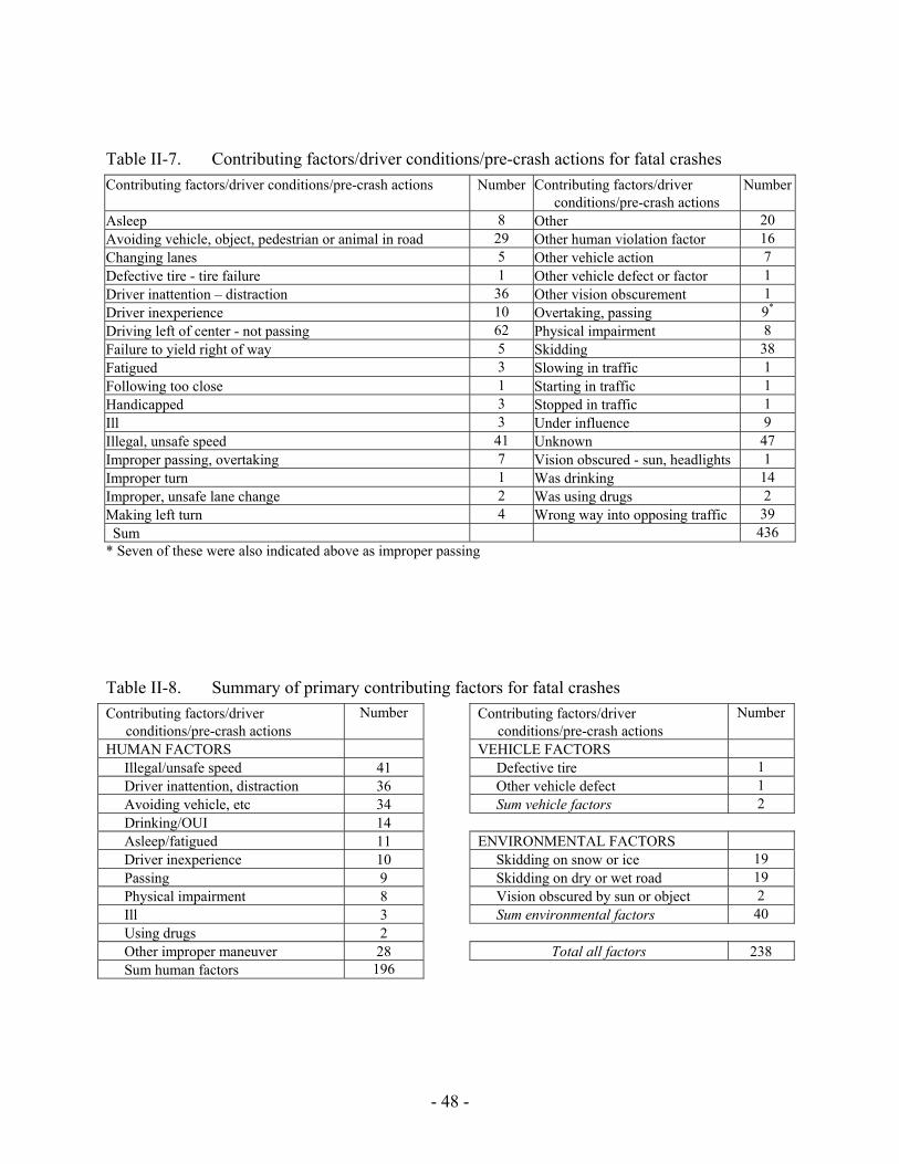
- 48 -

Table II-7. Contributing factors/driver conditions/pre-crash actions for fatal crashes Contributing factors/driver conditions/pre-crash actions Number Contributing factors/driver

conditions/pre-crash actions Number

Asleep 8 Other 20 Avoiding vehicle, object, pedestrian or animal in road 29 Other human violation factor 16 Changing lanes 5 Other vehicle action 7 Defective tire - tire failure 1 Other vehicle defect or factor 1 Driver inattention – distraction 36 Other vision obscurement 1 Driver inexperience 10 Overtaking, passing 9* Driving left of center - not passing 62 Physical impairment 8 Failure to yield right of way 5 Skidding 38 Fatigued 3 Slowing in traffic 1 Following too close 1 Starting in traffic 1 Handicapped 3 Stopped in traffic 1 Ill 3 Under influence 9 Illegal, unsafe speed 41 Unknown 47 Improper passing, overtaking 7 Vision obscured - sun, headlights 1 Improper turn 1 Was drinking 14 Improper, unsafe lane change 2 Was using drugs 2 Making left turn 4 Wrong way into opposing traffic 39 Sum 436

* Seven of these were also indicated above as improper passing

Table II-8. Summary of primary contributing factors for fatal crashes Contributing factors/driver

conditions/pre-crash actions Number Contributing factors/driver

conditions/pre-crash actions Number

HUMAN FACTORS VEHICLE FACTORS Illegal/unsafe speed 41 Defective tire 1 Driver inattention, distraction 36 Other vehicle defect 1 Avoiding vehicle, etc 34 Sum vehicle factors 2 Drinking/OUI 14 Asleep/fatigued 11 ENVIRONMENTAL FACTORS Driver inexperience 10 Skidding on snow or ice 19 Passing 9 Skidding on dry or wet road 19 Physical impairment 8 Vision obscured by sun or object 2 Ill 3 Sum environmental factors 40 Using drugs 2 Other improper maneuver 28 Total all factors 238 Sum human factors 196

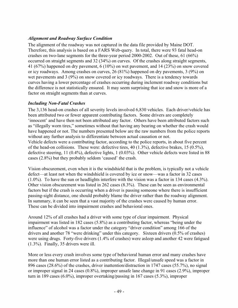
- 49 -

Alignment and Roadway Surface Condition The alignment of the roadway was not captured in the data file provided by Maine DOT. Therefore, this analysis is based on a FARS Web-query. In total, there were 93 fatal head-on crashes on two-lane segments for the three-year period 2000-2002. Out of these, 61 (66%) occurred on straight segments and 32 (34%) on curves. Of the crashes along straight segments, 41 (67%) happened on dry pavement, 6 (10%) on wet pavement, and 14 (23%) on snow covered or icy roadways. Among crashes on curves, 26 (81%) happened on dry pavements, 3 (9%) on wet pavements and 3 (9%) on snow covered or icy roadways. There is a tendency towards curves having a lower percentage of crashes occurring during inclement roadway conditions but the difference is not statistically ensured. It may seem surprising that ice and snow is more of a factor on straight segments than at curves.

Including Non-Fatal Crashes The 3,136 head-on crashes of all severity levels involved 6,830 vehicles. Each driver/vehicle has been attributed two or fewer apparent contributing factors. Some drivers are completely ‘innocent’ and have then not been attributed any factor. Others have been attributed factors such as “illegally worn tires,” sometimes without that having any bearing on whether the crash would have happened or not. The numbers presented below are the raw numbers from the police reports without any further analysis to differentiate between actual causation or not. Vehicle defects were a contributing factor, according to the police reports, in about five percent of the head-on collisions. These were: defective tires, 40 (1.3%), defective brakes, 15 (0.5%), defective steering, 11 (0.4%), defective lights, 1 (0.03%). Other vehicle defects were listed in 88 cases (2.8%) but they probably seldom ‘caused’ the crash. Vision obscurement, even when it is the windshield that is the problem, is typically not a vehicle defect—at least not when the windshield is covered by ice or snow—was a factor in 32 cases (1.0%). To have the sun or headlights interfere with the vision was a factor in 134 cases (4.3%). Other vision obscurement was listed in 262 cases (8.3%). These can be seen as environmental factors but if the crash is occurring when a driver is passing someone where there is insufficient passing-sight distance, one should probably blame the driver rather than the roadway alignment. In summary, it can be seen that a vast majority of the crashes were caused by human error. These can be divided into impairment crashes and behavioral ones. Around 12% of all crashes had a driver with some type of clear impairment. Physical impairment was listed in 182 cases (5.8%) as a contributing factor, whereas “being under the influence” of alcohol was a factor under the category “driver condition” among 166 of the drivers and another 78 “were drinking” under this category. Sixteen drivers (0.5% of crashes) were using drugs. Forty-five drivers (1.4% of crashes) were asleep and another 42 were fatigued (1.3%). Finally, 35 drivers were ill. More or less every crash involves some type of behavioral human error and many crashes have more than one human error listed as a contributing factor. Illegal/unsafe speed was a factor in 896 cases (28.6%) of the crashes, driver inattention/distraction in 1747 cases (55.7%), no signal or improper signal in 24 cases (0.8%), improper unsafe lane change in 91 cases (2.9%), improper turn in 189 cases (6.0%), improper overtaking/passing in 167 cases (5.3%), improper

- 50 -

park/start/stop in 111 cases (3.5%), following too closely in 88 cases (2.8%), failure to yield right-of-way in 1051 cases (33.5% of all crashes), driving left of center—not passing in 818 cases (26.1%), disregard of traffic control device in 149 cases (4.8%), and impeding traffic in 42 cases (1.3%). Driver inexperience was listed in 376 cases (12.0%), and “other human violation factor” in 359 cases (11.4%). Also, 202 drivers left the scene in hit-and-run crashes. Environmental factors with respect to roadway conditions are seldom listed as a contributing factor. However, every crash has roadway conditions and weather listed in the report and every driver has a pre-crash action listed—even if that entry often just states “following roadway.” The roadway was dry in 1759 crashes (56.1%), wet in 407 cases (13.0%), snow or ice covered and not sanded in 523 crashes (16.7%), sanded in 404 (12.9%) and had other or unknown conditions in the remaining 44 cases (1.4%). The pre-crash action shows that 627 drivers were skidding before they crashed (20.0% of all crashes), 654 drivers were making a left turn (20.9% of all crashes), 106 were making a right turn, 34 were making a U-turn, 136 (4.3%) were overtaking/passing, and 311 drivers (9.9%) were avoiding a vehicle, object, pedestrian or animal in road.

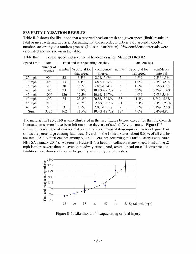
- 51 -

SEVERITY CAUSATION RESULTS Table II-9 shows the likelihood that a reported head-on crash at a given speed (limit) results in fatal or incapacitating injuries. Assuming that the recorded numbers vary around expected numbers according to a random process (Poisson distribution), 95% confidence intervals were calculated and are shown in the table. Table II-9. Posted speed and severity of head-on crashes, Maine 2000-2002

Fatal and incapacitating crashes Fatal crashes Speed limit Total number of

crashes number % of total for that speed

confidence interval

number % of total for that speed

confidence interval

25 mph 904 32 3.5% 2.5%-5.0% 5 0.6% 0.2%-1.3% 30 mph 204 13 6.4% 3.8%-10.6% 2 1.0% 0.3%-3.5% 35 mph 313 30 9.6% 6.8%-13.4% 5 1.6% 0.7%-3.7% 40 mph 146 23 15.8% 10.8%-22.7% 9 6.2% 3.3%-11.4% 45 mph 1006 126 12.5% 10.6%-14.7% 40 4.0% 2.9%-5.4% 50 mph 292 74 25.3% 20.8%-30.8% 33 11.3% 8.2%-15.5% 55 mph 216 61 28.2% 22.8%-34.7% 31 14.4% 10.4%-19.7% 65 mph 55 3 5.5% 2.0%-15.1% 2 3.6% 1.1%-12.5%

Sum 3136 362 11.5% 10.4%-12.7% 127 4.0% 3.4%-4.8% The material in Table II-9 is also illustrated in the two figures below, except for that the 65-mph Interstate crossovers have been left out since they are of such different nature. Figure II-3 shows the percentage of crashes that lead to fatal or incapacitating injuries whereas Figure II-4 shows the percentage causing fatalities. Overall in the United States, about 0.61% of all crashes are fatal (38,309 fatal crashes among 6,316,000 crashes according to Traffic Safety Facts 2002, NHTSA January 2004). As seen in Figure II-4, a head-on collision at any speed limit above 25 mph is more severe than the average roadway crash. And, overall, head-on collisions produce fatalities more than six times as frequently as other types of crashes.

0%

5%

10%

15%

20%

25%

30%

35%

30 40 50 Speed limit (mph)

Fata

l and

inca

paci

tatin

g in

jurie

s

25 35 45 55

Figure II-3. Likelihood of incapacitating or fatal injury

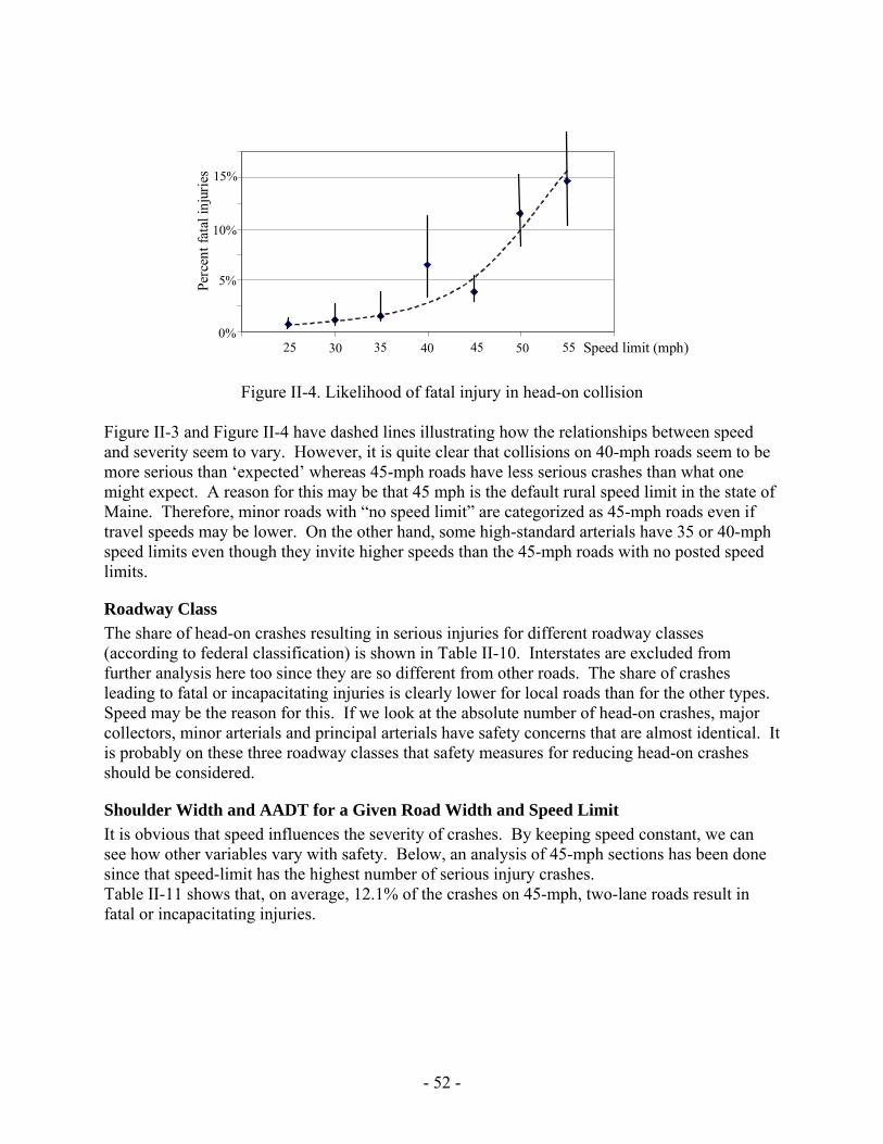
- 52 -

Figure II-4. Likelihood of fatal injury in head-on collision

Figure II-3 and Figure II-4 have dashed lines illustrating how the relationships between speed and severity seem to vary. However, it is quite clear that collisions on 40-mph roads seem to be more serious than ‘expected’ whereas 45-mph roads have less serious crashes than what one might expect. A reason for this may be that 45 mph is the default rural speed limit in the state of Maine. Therefore, minor roads with “no speed limit” are categorized as 45-mph roads even if travel speeds may be lower. On the other hand, some high-standard arterials have 35 or 40-mph speed limits even though they invite higher speeds than the 45-mph roads with no posted speed limits.

Roadway Class The share of head-on crashes resulting in serious injuries for different roadway classes (according to federal classification) is shown in Table II-10. Interstates are excluded from further analysis here too since they are so different from other roads. The share of crashes leading to fatal or incapacitating injuries is clearly lower for local roads than for the other types. Speed may be the reason for this. If we look at the absolute number of head-on crashes, major collectors, minor arterials and principal arterials have safety concerns that are almost identical. It is probably on these three roadway classes that safety measures for reducing head-on crashes should be considered.

Shoulder Width and AADT for a Given Road Width and Speed Limit It is obvious that speed influences the severity of crashes. By keeping speed constant, we can see how other variables vary with safety. Below, an analysis of 45-mph sections has been done since that speed-limit has the highest number of serious injury crashes. Table II-11 shows that, on average, 12.1% of the crashes on 45-mph, two-lane roads result in fatal or incapacitating injuries.

0%

5%

10%

15%

30 40 50 Speed limit (mph)

Perc

ent f

atal

inju

ries

25 35 45 55

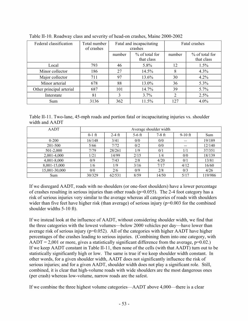
- 53 -

Table II-10. Roadway class and severity of head-on crashes, Maine 2000-2002 Fatal and incapacitating

crashes Fatal crashes Federal classification Total number

of crashes number % of total for

that class number % of total for

that class Local 793 46 5.8% 12 1.5%

Minor collector 186 27 14.5% 8 4.3% Major collector 711 97 13.6% 30 4.2% Minor arterial 678 88 13.0% 36 5.3%

Other principal arterial 687 101 14.7% 39 5.7% Interstate 81 3 3.7% 2 2.5%

Sum 3136 362 11.5% 127 4.0%

Table II-11. Two-lane, 45-mph roads and portion fatal or incapacitating injuries vs. shoulder width and AADT

Average shoulder width AADT 0-1 ft 2-4 ft 5-6 ft 7-8 ft 9-10 ft Sum

0-200 16/148 3/41 0/0 0/0 -- 19/189 201-500 5/66 7/72 0/2 0/0 -- 12/140

501-2,000 7/79 28/261 1/9 0/1 1/1 37/351 2,001-4,000 1/21 14/99 2/15 1/4 0/0 18/139 4,001-8,000 0/9 7/43 2/8 4/20 0/1 13/81

8,001-15,000 1/6 1/9 3/16 7/17 4/12 16/60 15,001-30,000 0/0 2/6 0/9 2/8 0/3 4/26

Sum 30/329 62/531 8/59 14/50 5/17 119/986 If we disregard AADT, roads with no shoulders (or one-foot shoulders) have a lower percentage of crashes resulting in serious injuries than other roads (p=0.055). The 2-4 foot category has a risk of serious injuries very similar to the average whereas all categories of roads with shoulders wider than five feet have higher risk (than average) of serious injury (p=0.003 for the combined shoulder widths 5-10 ft). If we instead look at the influence of AADT, without considering shoulder width, we find that the three categories with the lowest volumes—below 2000 vehicles per day—have lower than average risk of serious injury (p=0.052). All of the categories with higher AADT have higher percentages of the crashes leading to serious injuries. (Combining them into one category, with AADT = 2,001 or more, gives a statistically significant difference from the average, p=0.02.) If we keep AADT constant in Table II-11, then none of the cells (with that AADT) turn out to be statistically significantly high or low. The same is true if we keep shoulder width constant. In other words, for a given shoulder width, AADT does not significantly influence the risk of serious injuries; and for a given AADT, shoulder width does not play a significant role. Still, combined, it is clear that high-volume roads with wide shoulders are the most dangerous ones (per crash) whereas low-volume, narrow roads are the safest. If we combine the three highest volume categories—AADT above 4,000—there is a clear

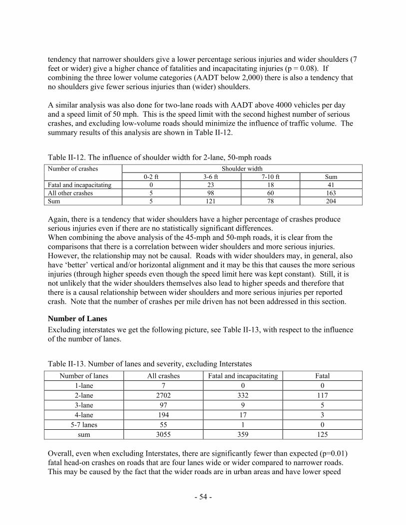
- 54 -

tendency that narrower shoulders give a lower percentage serious injuries and wider shoulders (7 feet or wider) give a higher chance of fatalities and incapacitating injuries (p = 0.08). If combining the three lower volume categories (AADT below 2,000) there is also a tendency that no shoulders give fewer serious injuries than (wider) shoulders. A similar analysis was also done for two-lane roads with AADT above 4000 vehicles per day and a speed limit of 50 mph. This is the speed limit with the second highest number of serious crashes, and excluding low-volume roads should minimize the influence of traffic volume. The summary results of this analysis are shown in Table II-12. Table II-12. The influence of shoulder width for 2-lane, 50-mph roads

Shoulder width Number of crashes 0-2 ft 3-6 ft 7-10 ft Sum

Fatal and incapacitating 0 23 18 41 All other crashes 5 98 60 163 Sum 5 121 78 204 Again, there is a tendency that wider shoulders have a higher percentage of crashes produce serious injuries even if there are no statistically significant differences. When combining the above analysis of the 45-mph and 50-mph roads, it is clear from the comparisons that there is a correlation between wider shoulders and more serious injuries. However, the relationship may not be causal. Roads with wider shoulders may, in general, also have ‘better’ vertical and/or horizontal alignment and it may be this that causes the more serious injuries (through higher speeds even though the speed limit here was kept constant). Still, it is not unlikely that the wider shoulders themselves also lead to higher speeds and therefore that there is a causal relationship between wider shoulders and more serious injuries per reported crash. Note that the number of crashes per mile driven has not been addressed in this section.

Number of Lanes Excluding interstates we get the following picture, see Table II-13, with respect to the influence of the number of lanes. Table II-13. Number of lanes and severity, excluding Interstates

Number of lanes All crashes Fatal and incapacitating Fatal 1-lane 7 0 0 2-lane 2702 332 117 3-lane 97 9 5 4-lane 194 17 3

5-7 lanes 55 1 0 sum 3055 359 125

Overall, even when excluding Interstates, there are significantly fewer than expected (p=0.01) fatal head-on crashes on roads that are four lanes wide or wider compared to narrower roads. This may be caused by the fact that the wider roads are in urban areas and have lower speed

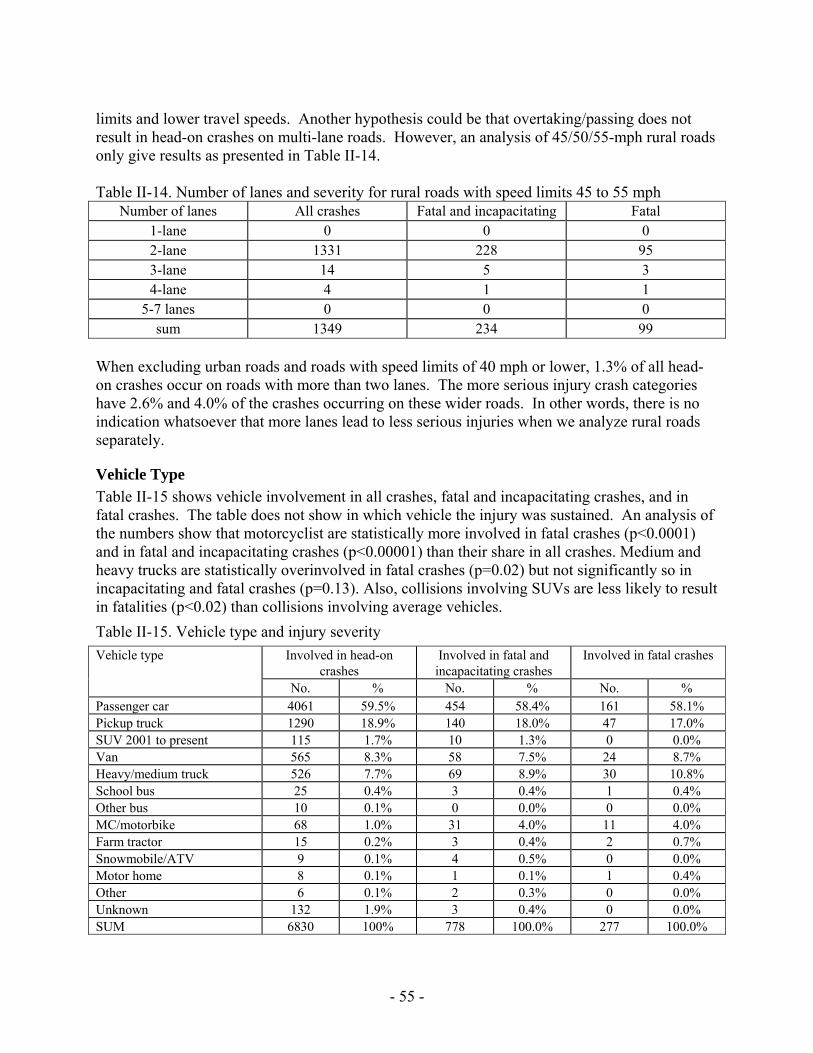
- 55 -

limits and lower travel speeds. Another hypothesis could be that overtaking/passing does not result in head-on crashes on multi-lane roads. However, an analysis of 45/50/55-mph rural roads only give results as presented in Table II-14. Table II-14. Number of lanes and severity for rural roads with speed limits 45 to 55 mph

Number of lanes All crashes Fatal and incapacitating Fatal 1-lane 0 0 0 2-lane 1331 228 95 3-lane 14 5 3 4-lane 4 1 1

5-7 lanes 0 0 0 sum 1349 234 99

When excluding urban roads and roads with speed limits of 40 mph or lower, 1.3% of all head-on crashes occur on roads with more than two lanes. The more serious injury crash categories have 2.6% and 4.0% of the crashes occurring on these wider roads. In other words, there is no indication whatsoever that more lanes lead to less serious injuries when we analyze rural roads separately.

Vehicle Type Table II-15 shows vehicle involvement in all crashes, fatal and incapacitating crashes, and in fatal crashes. The table does not show in which vehicle the injury was sustained. An analysis of the numbers show that motorcyclist are statistically more involved in fatal crashes (p<0.0001) and in fatal and incapacitating crashes (p<0.00001) than their share in all crashes. Medium and heavy trucks are statistically overinvolved in fatal crashes (p=0.02) but not significantly so in incapacitating and fatal crashes (p=0.13). Also, collisions involving SUVs are less likely to result in fatalities (p<0.02) than collisions involving average vehicles. Table II-15. Vehicle type and injury severity

Involved in head-on crashes

Involved in fatal and incapacitating crashes

Involved in fatal crashes Vehicle type

No. % No. % No. % Passenger car 4061 59.5% 454 58.4% 161 58.1% Pickup truck 1290 18.9% 140 18.0% 47 17.0% SUV 2001 to present 115 1.7% 10 1.3% 0 0.0% Van 565 8.3% 58 7.5% 24 8.7% Heavy/medium truck 526 7.7% 69 8.9% 30 10.8% School bus 25 0.4% 3 0.4% 1 0.4% Other bus 10 0.1% 0 0.0% 0 0.0% MC/motorbike 68 1.0% 31 4.0% 11 4.0% Farm tractor 15 0.2% 3 0.4% 2 0.7% Snowmobile/ATV 9 0.1% 4 0.5% 0 0.0% Motor home 8 0.1% 1 0.1% 1 0.4% Other 6 0.1% 2 0.3% 0 0.0% Unknown 132 1.9% 3 0.4% 0 0.0% SUM 6830 100% 778 100.0% 277 100.0%

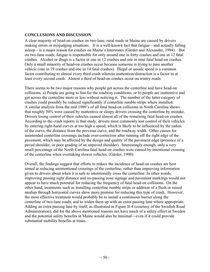
- 56 -

CONCLUSIONS AND DISCUSSION A clear majority of head-on crashes on two-lane, rural roads in Maine are caused by drivers making errors or misjudging situations. It is a well-known fact that fatigue—and actually falling asleep—is a major reason for crashes on Maine’s Interstates (Gårder and Alexander, 1994). But on two-lane roads, fatigue is responsible for only around one in forty crashes and one in 12 fatal crashes. Alcohol or drugs is a factor in one in 12 crashes and one in nine fatal head-on crashes. Only a small minority of head-on crashes occur because someone is trying to pass another vehicle (one in 19 crashes and one in 14 fatal crashes). Illegal or unsafe speed is a common factor contributing to almost every third crash whereas inattention/distraction is a factor in at least every second crash. Almost a third of head-on crashes occur on wintry roads. There seems to be two major reasons why people get across the centerline and have head-on collisions: a) People are going to fast for the roadway conditions; or b) people are inattentive and get across the centerline more or less without noticing it. The number of the latter category of crashes could possibly be reduced significantly if centerline rumble-strips where installed. A similar analysis from the mid 1980’s of all fatal head-on collisions in North Carolina shows that roughly 50% were caused by inattentive or sleepy drivers crossing the centerline by mistake. Drivers losing control of their vehicles caused almost all of the remaining fatal head-on crashes. According to the crash reports in that study, drivers most commonly lost control of their vehicles by entering right-hand curves at too high a speed, which is likely to be influenced by the radius of the curve, the distance from the previous curve, and the roadway width. Other causes for unintended centerline crossings include over-correction after running off the right edge of the pavement, which may be affected by the design and quality of the pavement edge (presence of a paved shoulder, or poor grading of an unpaved shoulder). Interestingly enough, only a very small percentage of the North Carolina fatal head-on crashes were caused by intentional crossing of the centerline when overtaking slower vehicles. (Gårder, 1990) Overall, the findings suggest that efforts to reduce the incidence of head-on crashes are best aimed at reducing unintentional crossings of the centerline, rather than improving information given to drivers about when it is safe to intentionally cross the centerline. In other words, improving passing sight distance and no-passing zone signage and pavement markings would not appear to have much potential for reducing the frequency of fatal head-on collisions. On the other hand, treatments such as installing centerline rumble strips or addition of a flush or raised median through horizontal curves show more promise for reducing this type of crash. However, the most effective treatment would probably be to install a continuous barrier along the centerline of two-lane roads, and to widen them up with an extra passing lane where appropriate. Adding an extra passing lane by itself, as illustrated in Figure II-4 (courtesy of the Swedish Road Administration), did for the above mentioned reasons not have much of a safety effect in Sweden and the potential safety benefits in Maine would also be minimal—even if it could provide substantial mobility benefits at times.

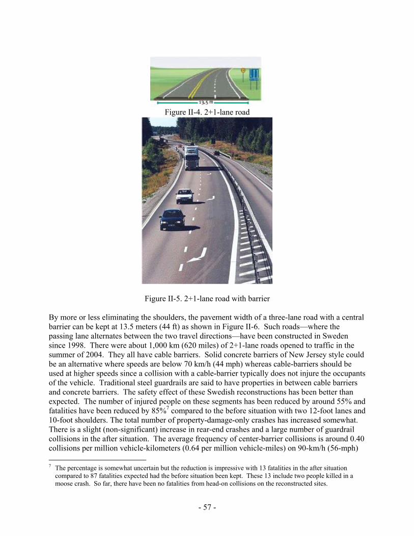
- 57 -

Figure II-4. 2+1-lane road

Figure II-5. 2+1-lane road with barrier By more or less eliminating the shoulders, the pavement width of a three-lane road with a central barrier can be kept at 13.5 meters (44 ft) as shown in Figure II-6. Such roads—where the passing lane alternates between the two travel directions—have been constructed in Sweden since 1998. There were about 1,000 km (620 miles) of 2+1-lane roads opened to traffic in the summer of 2004. They all have cable barriers. Solid concrete barriers of New Jersey style could be an alternative where speeds are below 70 km/h (44 mph) whereas cable-barriers should be used at higher speeds since a collision with a cable-barrier typically does not injure the occupants of the vehicle. Traditional steel guardrails are said to have properties in between cable barriers and concrete barriers. The safety effect of these Swedish reconstructions has been better than expected. The number of injured people on these segments has been reduced by around 55% and fatalities have been reduced by 85%7 compared to the before situation with two 12-foot lanes and 10-foot shoulders. The total number of property-damage-only crashes has increased somewhat. There is a slight (non-significant) increase in rear-end crashes and a large number of guardrail collisions in the after situation. The average frequency of center-barrier collisions is around 0.40 collisions per million vehicle-kilometers (0.64 per million vehicle-miles) on 90-km/h (56-mph) 7 The percentage is somewhat uncertain but the reduction is impressive with 13 fatalities in the after situation

compared to 87 fatalities expected had the before situation been kept. These 13 include two people killed in a moose crash. So far, there have been no fatalities from head-on collisions on the reconstructed sites.

- 58 -

roads and 0.56 collisions per million vehicle-kilometers (1.03 per million vehicle-miles) on 110-km/h (68-mph) roads. The cost of repairing the damages from approximately 3,000 barrier collisions8 has been substantial—not least from a worker-safety perspective—but at this point, no serious injuries have occurred during these repairs while more than 40 fatalities in head-on collisions have been eliminated. The average repair costs are around 70,000 SEK per year and kilometer9, or $14,000 per mile and year10. Also, plowing and snow-removal costs have increased by around 7,000 SEK per year and kilometer, or $1,400 per mile and year. Finally, with respect to attitudes, when the first segment was built, less than 1% of Swedish drivers thought the design idea was good. But within one year, 40% of users supported the design concept and now a majority likes these roads. A remaining problem is that some drivers with epileptic tendencies say they are bothered by the shadows cast by the posts and that motorcyclists11 fear what could happen if they crash into the cable barrier. (Carlsson and Bergh, 2004) To get a large number of center-barriers installed in Maine is probably unrealistic no matter how effective they may be. As noted above, Maine has 5,544 miles of numbered routes and if installing centerline barriers costs $68,00012 per mile, 5,544 miles of roadway installations would cost around $377 million13. However, to have centerline barriers installed along some high-crash sections may be a realistic goal. Other sections could have continuous centerline rumble strips installed. For mobility reasons, two-lane roads with center barriers need passing lanes at regular intervals. An alternating passing lane and cable barriers can be provided within the footprint of a two-lane road with 10-foot wide shoulders if the shoulders are narrowed to about one foot each. However, bicyclists and other slow-moving traffic will frequently need wide shoulders to travel safely and 4-foot shoulders should still be provided if there aren’t alternative routes for bicyclists. Also, if former shoulders are to be used as travel lanes, their bearing capacity must be upgraded to carry trucks. To widen two-lane roads and provide extra travel lanes without providing center barriers seem to influence the crash severity negatively. And, if we keep AADT and speeds constant, there is a clear tendency that roads with no shoulders or narrow shoulders have crashes producing few serious injuries while roads with wider shoulders (7 feet or wider) give a higher risk of fatalities and incapacitating injuries. If we cannot put in center-barriers to ‘eliminate’ crossovers or

8 Typically, 10 to 14 posts need to be replaced. The passing lane is closed off while this work is undertaken 9 Only about 10% of this cost has been carried by the Road Administration. 90% has been paid for through driver

insurance 10 This can be compared to an annual maintenance and repair costs estimated at $2,014/km for a similar cable

system in the center of I-5 in Oregon according to “Three-Cable Barrier Makes I-5 Safer” in Oregon Department of Transportation Research Notes August 1998, which can be accessed at http://www.oregon.gov/ODOT/TD/TP_RES/research_notes/cable.pdf#search='cable%20barrier%20installation%20cost'

11 Through 2004, there hadn’t been any serious injuries among motorcyclists 12 Washington State Department of Transportation News 2002 “I-5 Cable Median Barrier in Northern Clark County

Saves Lives and Money,” can be accessed at http://www.wsdot.wa.gov/news/dec02/median_barrier_clarkcounty.htm

13 Maine Department of Transportation is budgeting $483 million for the entire program area Highways and Bridges for the fiscal biennium 2004-2005 according to the Biennial Transportation Improvement Program, Fiscal Years 2004-2005, Maine Department of Transportation

- 59 -

install centerline rumble strips to reduce involuntary crossovers caused by driver inattention, the most effective way of reducing crash severity, according to the data presented here, is to reduce speeds. However, it would be difficult to get acceptance among drivers in Maine for reducing speed limits across the board. And since two-thirds of all fatalities occur on straight segments, reducing the speed at sharp curves only would not be very effective. Rather, speed limits should be better enforced—or enforced through photo enforcement and/or in-vehicle technology—since a high percentage of serious crashes involve illegal speeding. This could be combined with lower speed limits for a few targeted high-crash segments.

- 60 -

REFERENCES FARS (2005), Fatality Analysis Reporting System (FARS) Web-Based Encyclopedia made available by NCSA (National Statistics for Statistics and Analysis) and NHTSA (National Highway Traffic Safety Administration) within the US Department of Transportation at http://www-fars.nhtsa.dot.gov/ FHWA (1994), Federal Highway Administration: Motor Vehicle Accident Costs, U.S. Department of Transportation, FHWA Technical Advisory T 7570.2 Gårder, Per (1990) Occurrence of Evasive Maneuvers Prior to Accidents-Data from North Carolina Accidents, Proceedings of the 2nd Workshop of the International Committee on Traffic Conflicts Techniques (ICTCT), Munich, Germany, November 23-24, 1989. Bulletin 86, 13 pages, Lund Institute of Technology, Lund, Sweden Carlsson, Arne and Bergh, Torsten (2004), 2+1 vägar med räcke. Väg- och Vattenbyggaren no. 6, 2004, Stockholm, Sweden Gårder, Per & Alexander, John (1994) Shoulder Rumble Strips for Improving Safety on Rural Interstates. Year One, Final report. Technical Paper 94-4. Technical Services Division, Maine Department of Transportation

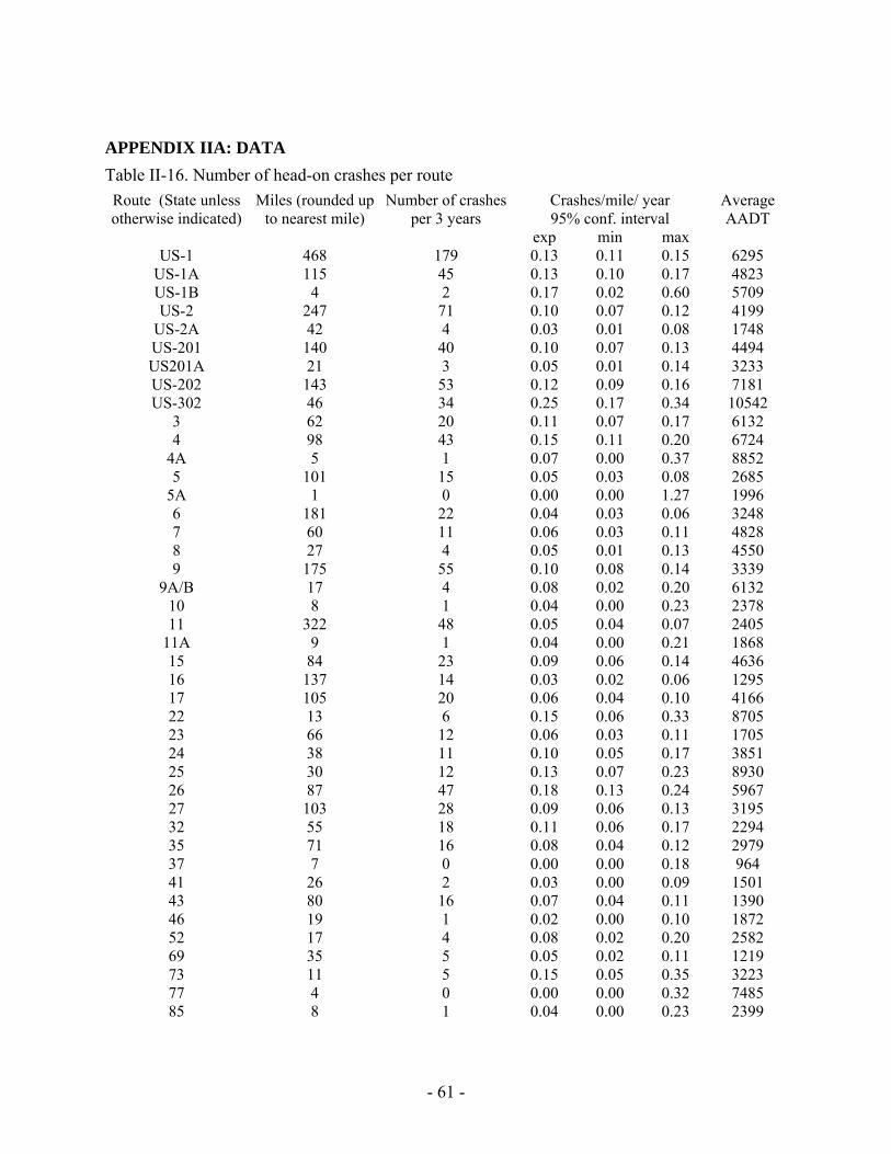
- 61 -

APPENDIX IIA: DATA Table II-16. Number of head-on crashes per route

Crashes/mile/ year 95% conf. interval

Route (State unless otherwise indicated)

Miles (rounded up to nearest mile)

Number of crashesper 3 years

exp min max

Average AADT

US-1 468 179 0.13 0.11 0.15 6295 US-1A 115 45 0.13 0.10 0.17 4823 US-1B 4 2 0.17 0.02 0.60 5709 US-2 247 71 0.10 0.07 0.12 4199

US-2A 42 4 0.03 0.01 0.08 1748 US-201 140 40 0.10 0.07 0.13 4494 US201A 21 3 0.05 0.01 0.14 3233 US-202 143 53 0.12 0.09 0.16 7181 US-302 46 34 0.25 0.17 0.34 10542

3 62 20 0.11 0.07 0.17 6132 4 98 43 0.15 0.11 0.20 6724

4A 5 1 0.07 0.00 0.37 8852 5 101 15 0.05 0.03 0.08 2685

5A 1 0 0.00 0.00 1.27 1996 6 181 22 0.04 0.03 0.06 3248 7 60 11 0.06 0.03 0.11 4828 8 27 4 0.05 0.01 0.13 4550 9 175 55 0.10 0.08 0.14 3339

9A/B 17 4 0.08 0.02 0.20 6132 10 8 1 0.04 0.00 0.23 2378 11 322 48 0.05 0.04 0.07 2405

11A 9 1 0.04 0.00 0.21 1868 15 84 23 0.09 0.06 0.14 4636 16 137 14 0.03 0.02 0.06 1295 17 105 20 0.06 0.04 0.10 4166 22 13 6 0.15 0.06 0.33 8705 23 66 12 0.06 0.03 0.11 1705 24 38 11 0.10 0.05 0.17 3851 25 30 12 0.13 0.07 0.23 8930 26 87 47 0.18 0.13 0.24 5967 27 103 28 0.09 0.06 0.13 3195 32 55 18 0.11 0.06 0.17 2294 35 71 16 0.08 0.04 0.12 2979 37 7 0 0.00 0.00 0.18 964 41 26 2 0.03 0.00 0.09 1501 43 80 16 0.07 0.04 0.11 1390 46 19 1 0.02 0.00 0.10 1872 52 17 4 0.08 0.02 0.20 2582 69 35 5 0.05 0.02 0.11 1219 73 11 5 0.15 0.05 0.35 3223 77 4 0 0.00 0.00 0.32 7485 85 8 1 0.04 0.00 0.23 2399

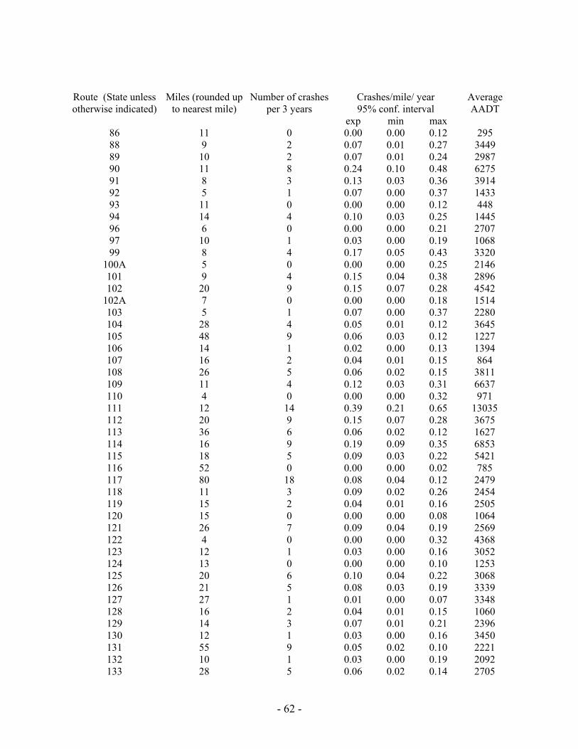
- 62 -

Crashes/mile/ year 95% conf. interval

Route (State unless otherwise indicated)

Miles (rounded up to nearest mile)

Number of crashesper 3 years

exp min max

Average AADT

86 11 0 0.00 0.00 0.12 295 88 9 2 0.07 0.01 0.27 3449 89 10 2 0.07 0.01 0.24 2987 90 11 8 0.24 0.10 0.48 6275 91 8 3 0.13 0.03 0.36 3914 92 5 1 0.07 0.00 0.37 1433 93 11 0 0.00 0.00 0.12 448 94 14 4 0.10 0.03 0.25 1445 96 6 0 0.00 0.00 0.21 2707 97 10 1 0.03 0.00 0.19 1068 99 8 4 0.17 0.05 0.43 3320

100A 5 0 0.00 0.00 0.25 2146 101 9 4 0.15 0.04 0.38 2896 102 20 9 0.15 0.07 0.28 4542

102A 7 0 0.00 0.00 0.18 1514 103 5 1 0.07 0.00 0.37 2280 104 28 4 0.05 0.01 0.12 3645 105 48 9 0.06 0.03 0.12 1227 106 14 1 0.02 0.00 0.13 1394 107 16 2 0.04 0.01 0.15 864 108 26 5 0.06 0.02 0.15 3811 109 11 4 0.12 0.03 0.31 6637 110 4 0 0.00 0.00 0.32 971 111 12 14 0.39 0.21 0.65 13035 112 20 9 0.15 0.07 0.28 3675 113 36 6 0.06 0.02 0.12 1627 114 16 9 0.19 0.09 0.35 6853 115 18 5 0.09 0.03 0.22 5421 116 52 0 0.00 0.00 0.02 785 117 80 18 0.08 0.04 0.12 2479 118 11 3 0.09 0.02 0.26 2454 119 15 2 0.04 0.01 0.16 2505 120 15 0 0.00 0.00 0.08 1064 121 26 7 0.09 0.04 0.19 2569 122 4 0 0.00 0.00 0.32 4368 123 12 1 0.03 0.00 0.16 3052 124 13 0 0.00 0.00 0.10 1253 125 20 6 0.10 0.04 0.22 3068 126 21 5 0.08 0.03 0.19 3339 127 27 1 0.01 0.00 0.07 3348 128 16 2 0.04 0.01 0.15 1060 129 14 3 0.07 0.01 0.21 2396 130 12 1 0.03 0.00 0.16 3450 131 55 9 0.05 0.02 0.10 2221 132 10 1 0.03 0.00 0.19 2092 133 28 5 0.06 0.02 0.14 2705

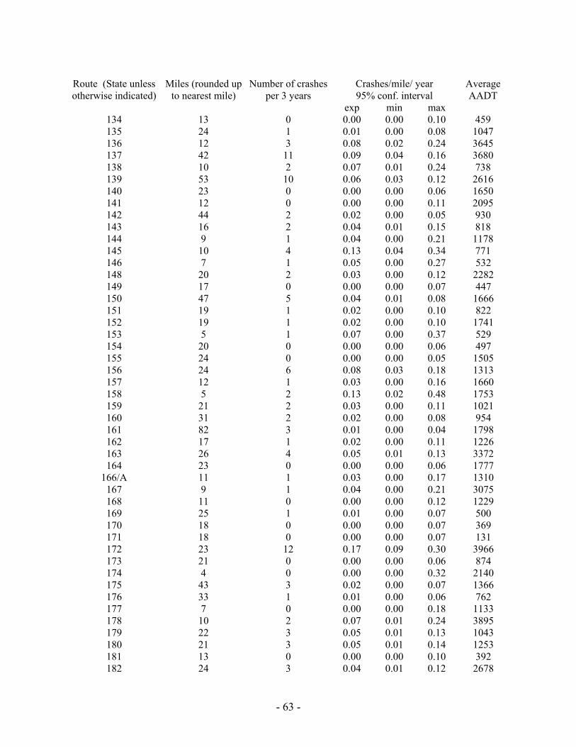
- 63 -

Crashes/mile/ year 95% conf. interval

Route (State unless otherwise indicated)

Miles (rounded up to nearest mile)

Number of crashesper 3 years

exp min max

Average AADT

134 13 0 0.00 0.00 0.10 459 135 24 1 0.01 0.00 0.08 1047 136 12 3 0.08 0.02 0.24 3645 137 42 11 0.09 0.04 0.16 3680 138 10 2 0.07 0.01 0.24 738 139 53 10 0.06 0.03 0.12 2616 140 23 0 0.00 0.00 0.06 1650 141 12 0 0.00 0.00 0.11 2095 142 44 2 0.02 0.00 0.05 930 143 16 2 0.04 0.01 0.15 818 144 9 1 0.04 0.00 0.21 1178 145 10 4 0.13 0.04 0.34 771 146 7 1 0.05 0.00 0.27 532 148 20 2 0.03 0.00 0.12 2282 149 17 0 0.00 0.00 0.07 447 150 47 5 0.04 0.01 0.08 1666 151 19 1 0.02 0.00 0.10 822 152 19 1 0.02 0.00 0.10 1741 153 5 1 0.07 0.00 0.37 529 154 20 0 0.00 0.00 0.06 497 155 24 0 0.00 0.00 0.05 1505 156 24 6 0.08 0.03 0.18 1313 157 12 1 0.03 0.00 0.16 1660 158 5 2 0.13 0.02 0.48 1753 159 21 2 0.03 0.00 0.11 1021 160 31 2 0.02 0.00 0.08 954 161 82 3 0.01 0.00 0.04 1798 162 17 1 0.02 0.00 0.11 1226 163 26 4 0.05 0.01 0.13 3372 164 23 0 0.00 0.00 0.06 1777

166/A 11 1 0.03 0.00 0.17 1310 167 9 1 0.04 0.00 0.21 3075 168 11 0 0.00 0.00 0.12 1229 169 25 1 0.01 0.00 0.07 500 170 18 0 0.00 0.00 0.07 369 171 18 0 0.00 0.00 0.07 131 172 23 12 0.17 0.09 0.30 3966 173 21 0 0.00 0.00 0.06 874 174 4 0 0.00 0.00 0.32 2140 175 43 3 0.02 0.00 0.07 1366 176 33 1 0.01 0.00 0.06 762 177 7 0 0.00 0.00 0.18 1133 178 10 2 0.07 0.01 0.24 3895 179 22 3 0.05 0.01 0.13 1043 180 21 3 0.05 0.01 0.14 1253 181 13 0 0.00 0.00 0.10 392 182 24 3 0.04 0.01 0.12 2678

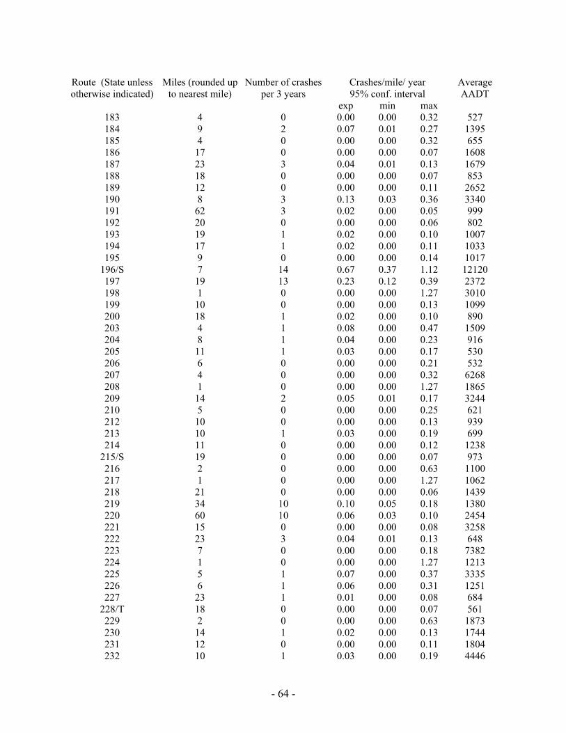
- 64 -

Route (State unless otherwise indicated)

Miles (rounded up to nearest mile)

Number of crashesper 3 years

Crashes/mile/ year 95% conf. interval

Average AADT

exp min max 183 4 0 0.00 0.00 0.32 527 184 9 2 0.07 0.01 0.27 1395 185 4 0 0.00 0.00 0.32 655 186 17 0 0.00 0.00 0.07 1608 187 23 3 0.04 0.01 0.13 1679 188 18 0 0.00 0.00 0.07 853 189 12 0 0.00 0.00 0.11 2652 190 8 3 0.13 0.03 0.36 3340 191 62 3 0.02 0.00 0.05 999 192 20 0 0.00 0.00 0.06 802 193 19 1 0.02 0.00 0.10 1007 194 17 1 0.02 0.00 0.11 1033 195 9 0 0.00 0.00 0.14 1017

196/S 7 14 0.67 0.37 1.12 12120 197 19 13 0.23 0.12 0.39 2372 198 1 0 0.00 0.00 1.27 3010 199 10 0 0.00 0.00 0.13 1099 200 18 1 0.02 0.00 0.10 890 203 4 1 0.08 0.00 0.47 1509 204 8 1 0.04 0.00 0.23 916 205 11 1 0.03 0.00 0.17 530 206 6 0 0.00 0.00 0.21 532 207 4 0 0.00 0.00 0.32 6268 208 1 0 0.00 0.00 1.27 1865 209 14 2 0.05 0.01 0.17 3244 210 5 0 0.00 0.00 0.25 621 212 10 0 0.00 0.00 0.13 939 213 10 1 0.03 0.00 0.19 699 214 11 0 0.00 0.00 0.12 1238

215/S 19 0 0.00 0.00 0.07 973 216 2 0 0.00 0.00 0.63 1100 217 1 0 0.00 0.00 1.27 1062 218 21 0 0.00 0.00 0.06 1439 219 34 10 0.10 0.05 0.18 1380 220 60 10 0.06 0.03 0.10 2454 221 15 0 0.00 0.00 0.08 3258 222 23 3 0.04 0.01 0.13 648 223 7 0 0.00 0.00 0.18 7382 224 1 0 0.00 0.00 1.27 1213 225 5 1 0.07 0.00 0.37 3335 226 6 1 0.06 0.00 0.31 1251 227 23 1 0.01 0.00 0.08 684

228/T 18 0 0.00 0.00 0.07 561 229 2 0 0.00 0.00 0.63 1873 230 14 1 0.02 0.00 0.13 1744 231 12 0 0.00 0.00 0.11 1804 232 10 1 0.03 0.00 0.19 4446

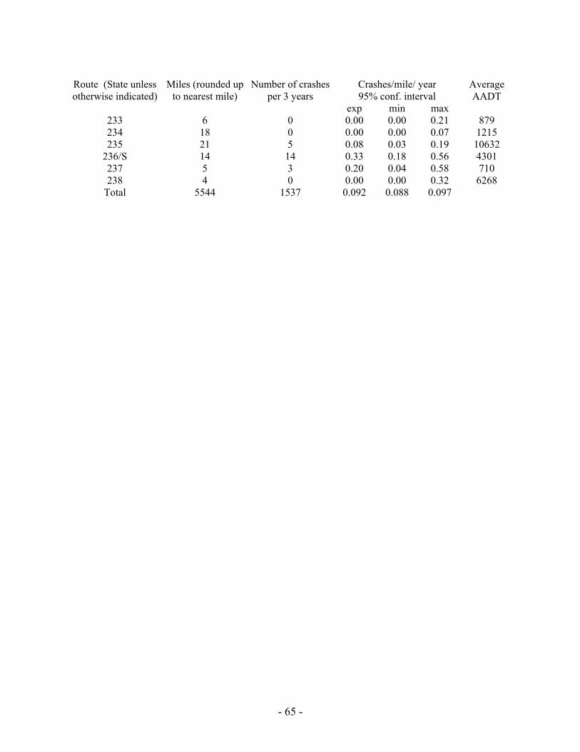
- 65 -

Route (State unless otherwise indicated)

Miles (rounded up to nearest mile)

Number of crashesper 3 years

Crashes/mile/ year 95% conf. interval

Average AADT

exp min max 233 6 0 0.00 0.00 0.21 879 234 18 0 0.00 0.00 0.07 1215 235 21 5 0.08 0.03 0.19 10632

236/S 14 14 0.33 0.18 0.56 4301 237 5 3 0.20 0.04 0.58 710 238 4 0 0.00 0.00 0.32 6268

Total 5544 1537 0.092 0.088 0.097

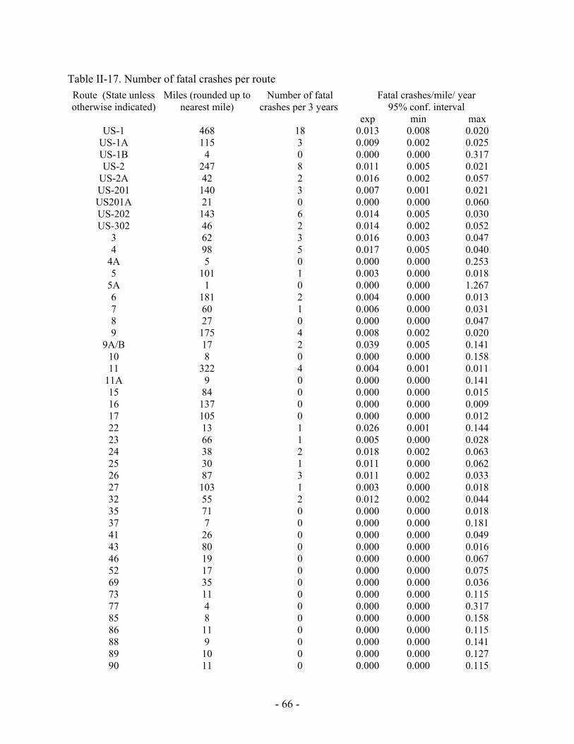
- 66 -

Table II-17. Number of fatal crashes per route Fatal crashes/mile/ year

95% conf. interval Route (State unless otherwise indicated)

Miles (rounded up to nearest mile)

Number of fatal crashes per 3 years

exp min max US-1 468 18 0.013 0.008 0.020

US-1A 115 3 0.009 0.002 0.025 US-1B 4 0 0.000 0.000 0.317 US-2 247 8 0.011 0.005 0.021

US-2A 42 2 0.016 0.002 0.057 US-201 140 3 0.007 0.001 0.021 US201A 21 0 0.000 0.000 0.060 US-202 143 6 0.014 0.005 0.030 US-302 46 2 0.014 0.002 0.052

3 62 3 0.016 0.003 0.047 4 98 5 0.017 0.005 0.040

4A 5 0 0.000 0.000 0.253 5 101 1 0.003 0.000 0.018

5A 1 0 0.000 0.000 1.267 6 181 2 0.004 0.000 0.013 7 60 1 0.006 0.000 0.031 8 27 0 0.000 0.000 0.047 9 175 4 0.008 0.002 0.020

9A/B 17 2 0.039 0.005 0.141 10 8 0 0.000 0.000 0.158 11 322 4 0.004 0.001 0.011

11A 9 0 0.000 0.000 0.141 15 84 0 0.000 0.000 0.015 16 137 0 0.000 0.000 0.009 17 105 0 0.000 0.000 0.012 22 13 1 0.026 0.001 0.144 23 66 1 0.005 0.000 0.028 24 38 2 0.018 0.002 0.063 25 30 1 0.011 0.000 0.062 26 87 3 0.011 0.002 0.033 27 103 1 0.003 0.000 0.018 32 55 2 0.012 0.002 0.044 35 71 0 0.000 0.000 0.018 37 7 0 0.000 0.000 0.181 41 26 0 0.000 0.000 0.049 43 80 0 0.000 0.000 0.016 46 19 0 0.000 0.000 0.067 52 17 0 0.000 0.000 0.075 69 35 0 0.000 0.000 0.036 73 11 0 0.000 0.000 0.115 77 4 0 0.000 0.000 0.317 85 8 0 0.000 0.000 0.158 86 11 0 0.000 0.000 0.115 88 9 0 0.000 0.000 0.141 89 10 0 0.000 0.000 0.127 90 11 0 0.000 0.000 0.115

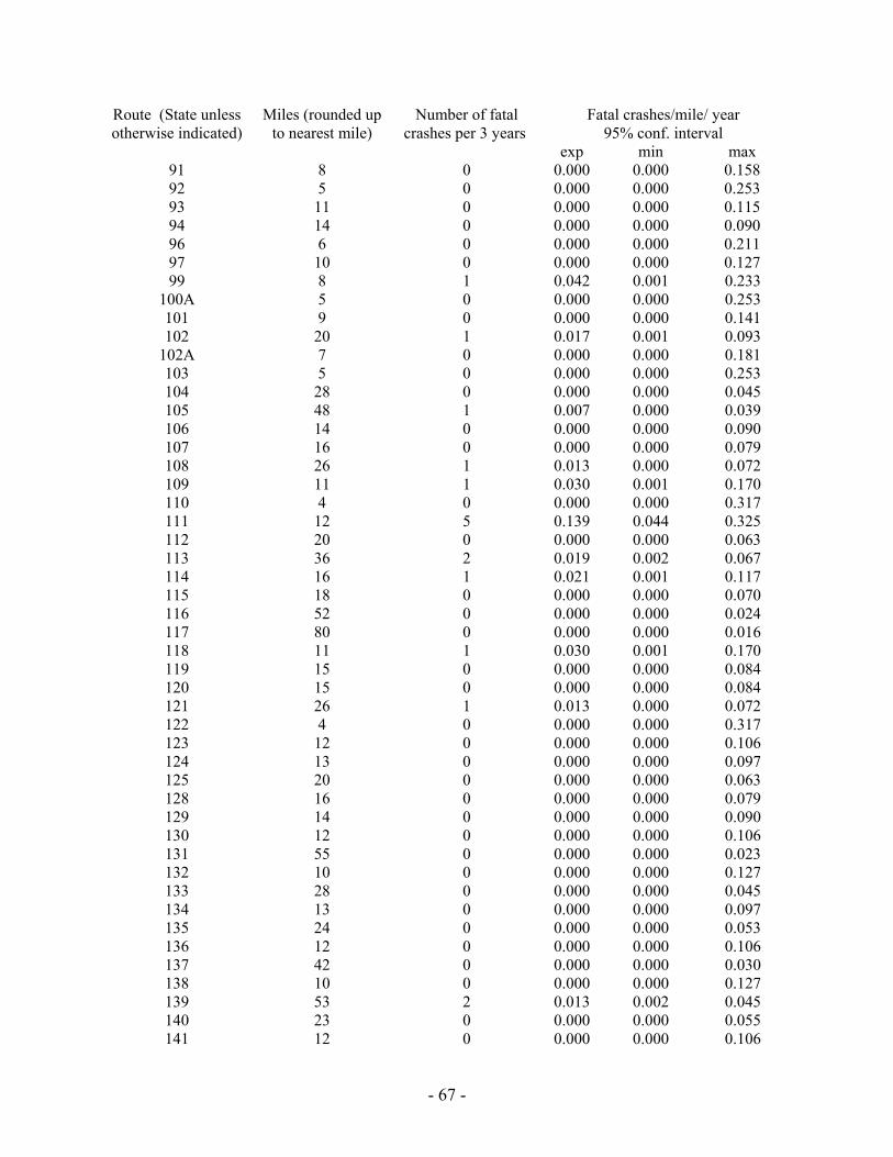
- 67 -

Route (State unless otherwise indicated)

Miles (rounded up to nearest mile)

Number of fatal crashes per 3 years

Fatal crashes/mile/ year 95% conf. interval

exp min max 91 8 0 0.000 0.000 0.158 92 5 0 0.000 0.000 0.253 93 11 0 0.000 0.000 0.115 94 14 0 0.000 0.000 0.090 96 6 0 0.000 0.000 0.211 97 10 0 0.000 0.000 0.127 99 8 1 0.042 0.001 0.233

100A 5 0 0.000 0.000 0.253 101 9 0 0.000 0.000 0.141 102 20 1 0.017 0.001 0.093

102A 7 0 0.000 0.000 0.181 103 5 0 0.000 0.000 0.253 104 28 0 0.000 0.000 0.045 105 48 1 0.007 0.000 0.039 106 14 0 0.000 0.000 0.090 107 16 0 0.000 0.000 0.079 108 26 1 0.013 0.000 0.072 109 11 1 0.030 0.001 0.170 110 4 0 0.000 0.000 0.317 111 12 5 0.139 0.044 0.325 112 20 0 0.000 0.000 0.063 113 36 2 0.019 0.002 0.067 114 16 1 0.021 0.001 0.117 115 18 0 0.000 0.000 0.070 116 52 0 0.000 0.000 0.024 117 80 0 0.000 0.000 0.016 118 11 1 0.030 0.001 0.170 119 15 0 0.000 0.000 0.084 120 15 0 0.000 0.000 0.084 121 26 1 0.013 0.000 0.072 122 4 0 0.000 0.000 0.317 123 12 0 0.000 0.000 0.106 124 13 0 0.000 0.000 0.097 125 20 0 0.000 0.000 0.063 128 16 0 0.000 0.000 0.079 129 14 0 0.000 0.000 0.090 130 12 0 0.000 0.000 0.106 131 55 0 0.000 0.000 0.023 132 10 0 0.000 0.000 0.127 133 28 0 0.000 0.000 0.045 134 13 0 0.000 0.000 0.097 135 24 0 0.000 0.000 0.053 136 12 0 0.000 0.000 0.106 137 42 0 0.000 0.000 0.030 138 10 0 0.000 0.000 0.127 139 53 2 0.013 0.002 0.045 140 23 0 0.000 0.000 0.055 141 12 0 0.000 0.000 0.106

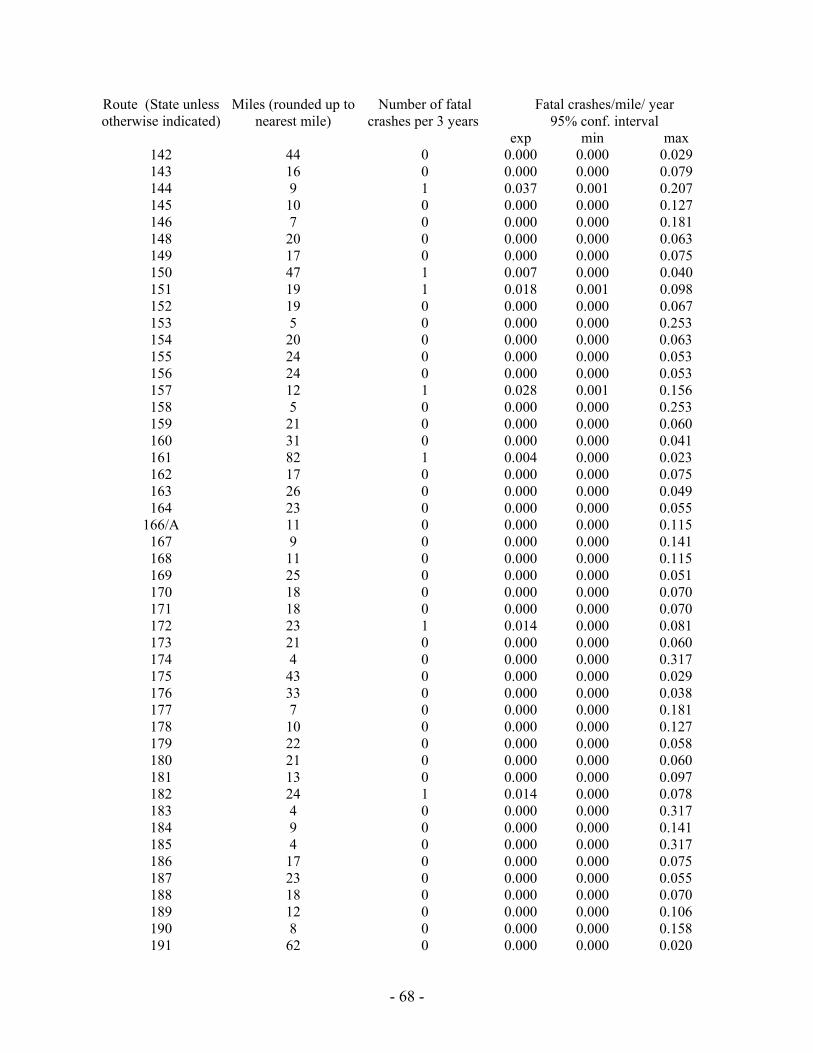
- 68 -

Route (State unless otherwise indicated)

Miles (rounded up to nearest mile)

Number of fatal crashes per 3 years

Fatal crashes/mile/ year 95% conf. interval

exp min max 142 44 0 0.000 0.000 0.029 143 16 0 0.000 0.000 0.079 144 9 1 0.037 0.001 0.207 145 10 0 0.000 0.000 0.127 146 7 0 0.000 0.000 0.181 148 20 0 0.000 0.000 0.063 149 17 0 0.000 0.000 0.075 150 47 1 0.007 0.000 0.040 151 19 1 0.018 0.001 0.098 152 19 0 0.000 0.000 0.067 153 5 0 0.000 0.000 0.253 154 20 0 0.000 0.000 0.063 155 24 0 0.000 0.000 0.053 156 24 0 0.000 0.000 0.053 157 12 1 0.028 0.001 0.156 158 5 0 0.000 0.000 0.253 159 21 0 0.000 0.000 0.060 160 31 0 0.000 0.000 0.041 161 82 1 0.004 0.000 0.023 162 17 0 0.000 0.000 0.075 163 26 0 0.000 0.000 0.049 164 23 0 0.000 0.000 0.055

166/A 11 0 0.000 0.000 0.115 167 9 0 0.000 0.000 0.141 168 11 0 0.000 0.000 0.115 169 25 0 0.000 0.000 0.051 170 18 0 0.000 0.000 0.070 171 18 0 0.000 0.000 0.070 172 23 1 0.014 0.000 0.081 173 21 0 0.000 0.000 0.060 174 4 0 0.000 0.000 0.317 175 43 0 0.000 0.000 0.029 176 33 0 0.000 0.000 0.038 177 7 0 0.000 0.000 0.181 178 10 0 0.000 0.000 0.127 179 22 0 0.000 0.000 0.058 180 21 0 0.000 0.000 0.060 181 13 0 0.000 0.000 0.097 182 24 1 0.014 0.000 0.078 183 4 0 0.000 0.000 0.317 184 9 0 0.000 0.000 0.141 185 4 0 0.000 0.000 0.317 186 17 0 0.000 0.000 0.075 187 23 0 0.000 0.000 0.055 188 18 0 0.000 0.000 0.070 189 12 0 0.000 0.000 0.106 190 8 0 0.000 0.000 0.158 191 62 0 0.000 0.000 0.020

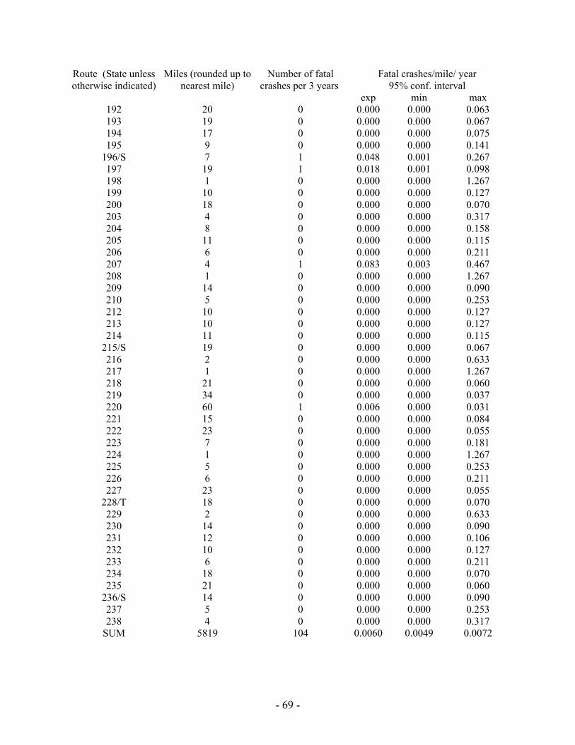
- 69 -

Route (State unless otherwise indicated)

Miles (rounded up to nearest mile)

Number of fatal crashes per 3 years

Fatal crashes/mile/ year 95% conf. interval

exp min max 192 20 0 0.000 0.000 0.063 193 19 0 0.000 0.000 0.067 194 17 0 0.000 0.000 0.075 195 9 0 0.000 0.000 0.141

196/S 7 1 0.048 0.001 0.267 197 19 1 0.018 0.001 0.098 198 1 0 0.000 0.000 1.267 199 10 0 0.000 0.000 0.127 200 18 0 0.000 0.000 0.070 203 4 0 0.000 0.000 0.317 204 8 0 0.000 0.000 0.158 205 11 0 0.000 0.000 0.115 206 6 0 0.000 0.000 0.211 207 4 1 0.083 0.003 0.467 208 1 0 0.000 0.000 1.267 209 14 0 0.000 0.000 0.090 210 5 0 0.000 0.000 0.253 212 10 0 0.000 0.000 0.127 213 10 0 0.000 0.000 0.127 214 11 0 0.000 0.000 0.115

215/S 19 0 0.000 0.000 0.067 216 2 0 0.000 0.000 0.633 217 1 0 0.000 0.000 1.267 218 21 0 0.000 0.000 0.060 219 34 0 0.000 0.000 0.037 220 60 1 0.006 0.000 0.031 221 15 0 0.000 0.000 0.084 222 23 0 0.000 0.000 0.055 223 7 0 0.000 0.000 0.181 224 1 0 0.000 0.000 1.267 225 5 0 0.000 0.000 0.253 226 6 0 0.000 0.000 0.211 227 23 0 0.000 0.000 0.055

228/T 18 0 0.000 0.000 0.070 229 2 0 0.000 0.000 0.633 230 14 0 0.000 0.000 0.090 231 12 0 0.000 0.000 0.106 232 10 0 0.000 0.000 0.127 233 6 0 0.000 0.000 0.211 234 18 0 0.000 0.000 0.070 235 21 0 0.000 0.000 0.060

236/S 14 0 0.000 0.000 0.090 237 5 0 0.000 0.000 0.253 238 4 0 0.000 0.000 0.317

SUM 5819 104 0.0060 0.0049 0.0072