J Econ Growth (2007) 12:235–259DOI 10.1007/s10887-007-9019-x

Inequality and mobility

John Hassler · José V. Rodríguez Mora · Joseph Zeira

Published online: 23 August 2007© Springer Science+Business Media, LLC 2007

Abstract Acknowledging that wage inequality and intergenerational mobility are stronglyinterrelated, this paper presents a model in which both are jointly determined. The modelenables us to study how inequality and mobility are affected by exogenous changes andwhat determines their correlation. A main implication of the model is that differences inthe amount of public subsidies to education and educational quality produce cross-countrypatterns with a negative correlation between inequality and mobility. Differences in the labormarket, like differences in skill-biased technology or wage compression instead produce apositive correlation. The predictions of the model are found to be consistent with variousempirical observations on mobility and inequality.

Keywords Intergenerational mobility · Inequality · Educational policy

J. Hassler (B)Institute for International Economics Studies (IIES), Stockholm University, Stockholm, Swedene-mail: John@hassler.se

J. Hassler · J. V. Rodríguez Mora · J. ZeiraCentre for Economic Policy Research, 53–56 Great Sutton Street, London, EC1V 0DG, UK

J. V. Rodríguez MoraUniversity of Southampton, Southampton, UKe-mail: sevimora@gmail.com

J. V. Rodríguez MoraUniversitat Pompeu Fabra, Barcelona, Spain

J. V. Rodríguez MoraUniversity of Edinburgh, Edinburgh, UK

J. ZeiraHebrew University of Jerusalem, Jerusalem, Israel

123

236 J Econ Growth (2007) 12:235–259

1 Introduction

Macroeconomic research on income inequality has expanded significantly in recent years.This interest in the distribution of income reflects both its social importance and also agrowing awareness among economists of its significant macroeconomic implications. In thispaper we claim that inequality, in particular wage inequality, should be analyzed jointly withintergenerational mobility, since the two are strongly related. On the one hand inequalityaffects mobility. A greater skill premium increases incentives for education acquisition andthus raises upward mobility and reduces downward mobility. On the other hand, intergener-ational mobility affects the supplies of skilled and unskilled and thus the returns to skill andwage inequality. This paper studies the general equilibrium determination of both.

The joint analysis of inequality and mobility is also important for a welfare analysis. Theutility of an individual depends on her current income, but also on the chances of herself orher children to change income in the future. Indirectly, individuals therefore care about futurerates of social mobility since high mobility means that a shock to the income of a dynastyis less persistent. In order to capture this, the model assumes that parents derive utility fromthe utility of their children. This enables the model to analyze how various policies affectwelfare through both inequality and mobility.

Finally and perhaps most importantly, our joint analysis of inequality and mobility canhelp in understanding various empirical findings. Our model predicts that differences in labormarkets across countries lead to a positive correlation between inequality and mobility. Ifcountries with high inequality also have high mobility, our model predicts that the main driv-ing force behind these differences is to be found at the labor market, e.g., different skill-biasin their industries or different labor market institutions. If instead a negative correlation isfound, the main difference is in the education system, e.g., the quality and general availabilityof public education. Thus, our model can contribute to understanding the underlying reasonsfor differences across countries in inequality and mobility.

Let us now describe the main ingredients of our model. Workers can be either skilled orunskilled and we use the ratio between their wages as a measure of inequality. This measureis endogenously determined in general equilibrium as a function of the relative supplies ofskilled and unskilled. Skill is acquired through education. We assume that parents cannot bor-row against the future income of their children and hence must finance education from theirincome only. The amount of education needed to become skilled differs both by the child’sinnate ability and by the parent’s education. The ability of an individual is stochastic and isindependent of parental ability. However, we assume that skilled parents have an advantageover unskilled parents in providing education for their children. For example, skilled parentshave better knowledge of what books to buy, which tutors to hire, or may provide a homeenvironment more suitable for education. As a result, success in education depends not onlyon ability but also on income of parents as well as on their education.

We assume that parents know the educational ability of their children. They allocateincome between their own consumption and their child’s education and that determines anability threshold above which children become skilled. These thresholds define the probabili-ties of becoming skilled and unskilled for children of various backgrounds. The probabilitiesdescribe intergenerational mobility in our model. The main variable we focus on is the prob-ability of a child of unskilled to become skilled, which is the rate of upward mobility. Weuse it as our main measure of mobility.

The equilibrium is analyzed by looking at two relationships between inequality and mobil-ity. The first describes how inequality affects the investment in education and thus the rateof upward mobility. We identify two potential and opposite effects here. On the one hand,

123

J Econ Growth (2007) 12:235–259 237

higher inequality increases the gains from education. This strengthens the incentive to investin education and increases upward mobility. We call this the incentive effect. On the otherhand, higher inequality reduces the ability of unskilled parents to pay for education costs thatare indexed to skilled wage, like teachers’ salaries. We call this negative effect of inequalityon mobility the distance effect. Note that even if all educational costs are indexed to unskilledwage, like foregone income, higher inequality still reduces the relative ability of unskilled topay for education. Namely, the difference in educational attainment between children withdifferent social backgrounds might increase with inequality.

The second equilibrium relationship reflects the effect of mobility on inequality throughthe production sector and the labor market. Higher mobility increases the net flow fromunskilled to skilled and reduces the number of unskilled in the long run. This raises theirwage, so it reduces inequality. Hence, this creates a negative relationship between mobilityand inequality.

The interaction of these two relationships determines the equilibrium. We then look at theeffect of various exogenous changes and divide them to two types: changes in the productionsector and changes in the education sector. Changes in the production sector tend to shiftinequality and mobility in the same direction. Intuitively, such changes affect the returns tofactors of production and thus affect inequality. Increased inequality tends to raise mobilitythrough the incentive effect and hence the correlation is positive. Changes in the educationsector usually lead to a negative correlation between inequality and mobility. Such changesincrease access to education and thus increase mobility. That reduces the number of unskilledworkers, which reduces inequality. Hence, the two variables are negatively related under suchchanges.

The paper then focuses on a public education, which is modeled as a subsidy to educa-tion. Similar to other improvements in education, a public subsidy reduces inequality andincreases upward mobility. As in Fernandez and Rogerson (1995), skilled parents have anadvantage in capturing the subsidy since they, on average, educate their children more. Thedirect effect of subsidies is therefore to increase the difference between educational attain-ment of children of skilled and of unskilled. However, in addition to previous literature, wealso consider the general equilibrium effect of the subsidy on wage inequality, through theincrease in supply of skill. The lower wage inequality reduces the difference in educationattainment between the two classes. Furthermore, we show that the indirect effect may verywell dominate the direct one and the long-run result of public education is a reduction ofthe difference in education attainment between children of skilled and of unskilled, unlikeprevious results in the literature.

Although measuring intergenerational mobility is hard, due to data limitations, empiricalresearch in the area has been growing recently, as more longitudinal data is being accumu-lated. We use this research to examine whether the predictions of our model are supported bythe data and we find significant support to it. Checchi et al. (1999) find that Italy is more equalbut less mobile than the US. Indeed, the fact that Italy has labor market policies which sig-nificantly compress wages relative to the US, fits this positive correlation between inequalityand mobility according to our model. Björklund et al. (2002) and Blanden et al. (2005) findthat Nordic countries and Canada are more equal and more mobile than the US and UK.Indeed, we show that public education is much larger in these countries than in US and UK,which should lead according to our model to a negative correlation between inequality andmobility. Dahan and Gaviria (2003) find that Latin American countries are both less equaland less mobile than the US. According to our model this hints at higher public education inthe US, which is found to be the case. We discuss other empirical findings as well and theyare largely in line with the predictions of our model.

123

238 J Econ Growth (2007) 12:235–259

This paper contributes to a growing literature that brings inequality and mobility into mac-roeconomics. This literature has been spurred by the recent widening of wage gaps, and byrecent findings that income distribution matters for the overall economy. This point has beenmade both theoretically, by Loury (1981), Galor and Zeira (1993), Banerjee and Newman(1993), Aghion and Bolton (1997), and others, and empirically by Alesina and Rodrik (1994),Persson and Tabellini (1994), Perotti (1996) and Barro (2000). Intergenerational mobility hasrecently been studied by Galor and Tsiddon (1997), Owen and Weil (1998), Fernandez andRogerson (1998), Maoz and Moav (1999), Hassler and Rodríguez Mora (2000), Benabou(2001) and Solon (2004). These studies focus mainly on the dynamics of inequality andmobility and their relation to economic growth. Recent papers, which focus on public educa-tion, are Glomm and Ravikumar (1992), Fernandez and Rogerson (1995), Benabou (2002)and Fender and Wang (2003).1

When placing our paper within this literature we wish to emphasize three important fea-tures of our model. The first is the question it raises. While most other papers discuss theevolution of inequality over time, our paper focuses on cross country differences in inequalityand mobility and enables us to draw empirical implications. The second special element ofthis model is the feedback from labor supplies to wage inequality. Most papers on inequalityand mobility study how wage levels affect skill acquisition. Few, however, allow the suppliesof skilled and unskilled labor to affect wages in general equilibrium on the labor market.2

The third special ingredient is the modeling of the intertemporal link within a dynasty byassuming that parents care about their offspring’s utility as in a Barro type model. Sharingformulation with the standard neoclassical macroeconomic model is an advantage in itself.More importantly, it adds new insights and results since it allows for the intuitive idea thatpeople care about inequality and mobility both current and future. These are the three specialingredients of our model, and although each appears in some papers, the integration of allthree elements into a unified theory of inequality and mobility has not been done previously.3

The paper is organized as follows. Section 2 presents the model, and Sect. 3 describesthe steady state equilibrium. Section 4 studies the comparative statics of the equilibriumwhile Sect. 5 analyzes the effects of public subsidies to education. Section 6 is devoted toan empirical discussion and Sect. 7 summarizes. The appendix contains some proofs and ananalysis of the case of no information on innate ability.

2 The model

Consider an economy that consists of two-period overlapping generations with no populationgrowth. Each person has one child, and each generation is a continuum of unitary measure.Individuals are born unskilled and in the first period of life they can acquire education andbecome skilled.

In the second period of life individuals supply inelastically one unit of labor, earningas skilled ws or wn as unskilled. They consume and invest in the education of their child,

1 Related are also two papers that deal with child labor and education policy: Baland and Robinson (2000)and Doepke and Zilibotti (2005).2 Exceptions are Galor and Zeira (1993), Owen and Weil (1998) and Maoz and Moav (1999).3 A cost of our approach is that we cannot analytically solve for the dynamics around the steady state. Weare also aware of the discussion about whether bequest incentives arise from the offspring’s utility or from the“warm glow of giving”. See, e.g., Altonji, et al. (1997). However, in our model parents directly finance theeducation of their children, in which case it is more reasonable to use the utilitarian assumption rather thanthe alternative.

123

J Econ Growth (2007) 12:235–259 239

deriving utility both from own consumption and from the expected utility of their offspring.Parental utility is:

ln c + βVoff ,

where c is own consumption, Voff is expected utility of offspring, and β ∈ (0, 1) is theintergenerational discount factor.

For wage determination we turn to describe production in the economy. There is one finalgood in the economy, which is produced with skilled and unskilled labor:

Y = F (a, N , S)

where N and S are the inputs of unskilled and skilled labor, respectively, F is a standardquasi-concave CRS production function of N and S, and a is a productivity parameter,which is assumed to affect skilled more than unskilled, as becomes clear below. Labor mar-kets are competitive and hence wages are equal to their respective marginal productivities.The skilled wages is ws = FS (a, N , S) = FS (a, n, 1), where n ≡ N/S is the relativesupply of unskilled workers. Similarly the unskilled wages is wn = FN (a, n, 1). Hence, theratio of skilled to unskilled wages, which is our measure of wage inequality and is denotedI , satisfies:

I ≡ ws

wn= FS (a, n, 1)

FN (a, n, 1)= I (a, n).

Due to quasi-concavity and CRS of the production function I is an increasing function of n.We can therefore write the inverse relation, namely how the labor supplies fit the equilibriumwage inequality, in the following way:

n = n (I, a) . (1)

We also assume that the range of I includes levels of inequality both above and belowunity, or formally, that limn→0 I (a, n) < 1 and limn→∞ I (a, n) > 1 for all relevant a′s.

As stated above, the productivity parameter a is assumed to be skill-biased. We formallyassume that the elasticity of FS with respect to a is larger than the elasticity of FN withrespect to a. This therefore means that Ia > 0, and also na < 0.

In most of the analysis in this paper, we use a CES specification of the production function

Y =(

Nσ−1σ + a

1σ S

σ−1σ

) σσ−1

, (2)

where σ is the elasticity of substitution between skilled and non-skilled labor. In this casewage inequality is described by the following function:

I = (an)1σ .

We next describe education acquisition. Children differ in the amount of education theyneed to become skilled, both due to different innate abilities to learn and to differences inparental education. The (inverse) measure of innate ability is “inaptitude.” It is the amountof education a child needs to become skilled if born to a skilled parent. We denote inaptitudeby e and assume that it is random, independent across families and over time, and distributeduniformly on [0, 1]. As we assume that educated parents help their children in non-pecuniaryways in addition to paying for education, children of unskilled parents face an educationalbarrier relative to children of skilled parents. A child with inaptitude e of an unskilled parentneeds be units of education to become skilled, where b ≥ 1. The barrier b reflects manyfactors, social, cultural, and even technological.

123

240 J Econ Growth (2007) 12:235–259

The cost of one unit of education is assumed to be proportional to the unskilled wage,namely it is wn

h , where h parameterizes the productivity of the educational sector. Thisassumption is a short-cut for a more detailed description of the educational production pro-cess, where a significant part of the cost is the opportunity cost of student time, which isproportional to the unskilled wage. We believe this assumption provides a reasonable baseline despite the fact that, literally, we do not have an opportunity cost of education in ourmodel. However, we have analyzed the case where education costs are indexed to skilledwages, finding similar results, except for very high inequality levels. We return to theseissues below.

Capital markets are imperfect. We assume that neither the parent nor the child can borrowto finance education and that dynasties can not accumulate wealth in order to finance educa-tion.4 As a result, parents pay for education out of their income. We assume first that educationis a private good, and introduce public education in Sect. 5. Regarding the information struc-ture of the model, we assume that the education decision is made after the child’s inaptitude isrevealed. Then the parent decides whether or not to spend the amount on education requiredto make the child skilled. In Appendix 2 we consider the case when the educational decisionis taken before information on inaptitude is revealed. In this case an interesting bargainingsituation emerges between parent and offspring, and as a result, intrafamily relations have aneffect on inequality and mobility.

3 Equilibrium

The decision to invest in the child’s education depends on the cost of education on the onehand and on the expected gains from education for the child on the other hand. Note that theinaptitude of the child is already known, so the expectation of gains refers to the yet unknowninaptitude of the grandchild and other future descendants. These gains depend of course onfuture wages for skilled and unskilled. To simplify the analysis we focus in the paper on thesteady state. Hence the expected utilities of skilled and unskilled are not time dependent andwe denote them by Vs and Vn , respectively, noting that these values are calculated before theaptitude of the child is revealed.

Suppose a parent with wage w has a child for whom it costs x to become educated. Theparent can decide to pay x and have a skilled offspring or to abstain and keep the offspringunskilled.5 Education is chosen if

ln(w − x) + βVs ≥ ln w + βVn .

Subtracting ln (w) from both sides we can derive a maximum share of the wage that aparent would pay to make her child skilled. We denote this maximum by m and note that itis determined by

4 There can be many reasons for the existence of the borrowing constraint. The main one is the inability todefine property rights, namely to commit the offspring to return loans taken by the parents. In fact, a perfectmarket in our model would require that a person must be able to commit his descendents in any future gener-ation. The inability to accumulate wealth is more restrictive and done to keep the analysis tractable. See alsonext footnote.5 Note that to keep the analysis tractable, we assume that a parent pays only to the child’s education and isnot allowed to leave an additional pecuniary bequest. It can be shown that this assumption is not needed andpeople do not leave an additional bequest if the steady state inequality satisfies: I (1 − β) > 1/h, which is inline with our parameterization below.

123

J Econ Growth (2007) 12:235–259 241

− ln(1 − m)

β= Vs − Vn . (3)

Hence, the log specification of utility implies that m is equal for skilled and unskilled anddepends only on the expected gains from education, namely on the RHS of (3).

Given a value of m, wages and the cost of education, we can now calculate threshold levelsof inaptitude for children of skilled and non-skilled such that if the inaptitude e is below thisthreshold, the parent will pay for her becoming skilled. The threshold level for children ofskilled is:

es = hm I (4)

and similarly, the education threshold for children of unskilled is:6

en = hm

b. (5)

The thresholds in Eqs. 4 and 5 are computed for a given level of m. This level will be deter-mined by the optimal choices of parents, as implicitly given by (3). As we will see shortly,this implies that m will be a monotone increasing function of I .

Note that given our distributional assumptions on e, the thresholds es and en are the sharesof children from skilled and non-skilled homes, respectively, who become skilled. Hence,1 − es and en are measures for downward and upward mobility, respectively. As we see,es ≥ en for two reasons. First, there is the direct social disadvantage if b > 1. Second, theincome difference affects the ability to pay for education. If I > 1 and b > 1, there is thus adouble relative handicap for children of non-skilled.

We next turn to calculate the expected gains from education, Vs − Vn , using the abovethreshold levels and the common value of m. The expected utility of skilled, before theirchild’s inaptitude becomes known, is

Vs =∫ es

0ln

(ws − e

wn

h

)de +

∫ 1

es

ln wsde + βVn + esβ (Vs − Vn). (6)

The last term represents the expected additional utility a skilled person gets from the pos-sibility that her child will become skilled. Calculating Vn in the same way and taking thedifference yields

Vs − Vn = ln I + ∫ es0 ln

(1 − e

I h

)de − ∫ en

0 ln(1 − e b

h

)de

1 − β (es − en).

As seen from this equation the gains from education include a direct income effect, as edu-cation raises income of the child, and an indirect effect, as an educated child will be able toprovide more education to her child, by avoiding the educational barrier.

Using the common value of m and evaluating the integrals,7 we can express the gainsfrom education as

Vs − Vn = ln I + h(I − 1

b

)(− (1 − m) ln (1 − m) − m)

1 − βh(I − 1

b

)m

. (7)

When m = 0, the gains from education are equal to ln I . As m rises and parents invest morein education, the gains from education may rise or decline.

6 If hm I ≥ 1, then es = 1 in a corner solution and all children of skilled become skilled themselves. Asshown later this is impossible in the steady state.7 Note that

∫ es0 ln

(1 − e

I h

)de = − (I h − es ) ln

(1 − es

I h

) − es .

123

242 J Econ Growth (2007) 12:235–259

Fig. 1 Incentive and gain fromeducation for given wageinequality

Vs V- n

Incentive

Gain

8.0

6.0

4.0

2.0

20.0 40.0 60.0 80.0 21.0 41.0 61.0 81.0 2.01.0m

Equations 3 and 7 describe two relationships between the gains to education and m. Equa-tion 3 describes how m depends on the gains from education and is drawn in Fig. 1 as themonotonically upward sloping Incentive curve. Equation 7 describes, instead, how the gainsfrom education depend on maximum educational spending m, and is drawn in Fig. 1 as theGain curve. The intersection of the two curves determines the steady state level of maximumspending on education m. Note that the denominator of the RHS of (7) is strictly positivesince βh

(I − 1

b

)m = β (es − en) < 1. In Fig. 1 we draw the two curves for the values

I = 1.55, h = 4, b = 1.1, β = 14 . In this example m is 0.107 and consequently, es = 0.663

and en = 0.389.The intersection of the incentive curve and the gain curve in Fig. 1 can be analytically

characterized by the following equation, which is derived from equating the LHS of (3) andthe RHS of (7):

− ln (1 − m)

β= ln I + h

(I − 1

b

)(− ln (1 − m) − m). (8)

This equation, which implicitly describes how the maximum investment in education dependson inequality, is analyzed in the following Proposition.

Proposition 1 For a given I , let m (I ) denote a solution to (8) such that es ∈ [0, 1] . It canthen be established that:

1. m (I ) exists for a non-degenerate domain I ∈ [1, Imax].2. m (I ) is unique.3. m (I ) is continuous and strictly increasing with m (1) = 0.

Proof in Appendix 1.According to Proposition 1 the maximum steady state spending on education m depends

positively on inequality I . Hence, upward mobility, which is:

en = M(I ) ≡ h

bm (I )

also depends positively on inequality. This is the incentive effect. It reflects how higherinequality increases the gains from education, increases the maximum spending on educa-tion and thus increases upward mobility. Note also that inequality reduces downward mobility,since 1 − es = 1 − hm (I ) I .

Clearly, income inequality and mobility are also related in the reverse direction, throughthe labor market. Mobility changes the supplies of skilled and unskilled, their wages and as

123

J Econ Growth (2007) 12:235–259 243

Fig. 2 Steady state equilibrium,en = L (I ) and en = M (I )

en

L(I )

M(I )6.0

5.0

4.0

3.0

2.0

1.0

2.1 4.1 6.1 8.1 2

I

a result wage inequality. To analyze it we focus on the steady state, in which the upward flowof children of unskilled, who acquire education, must equal the downward flow of childrenof skilled, who do not get education. The steady state must satisfy:

en N = (1 − es) S. (9)

We next show that our assumptions imply that the upward and downward flows in thesteady state are strictly positive. First note that es < 1. Otherwise, by (9) either N = 0 oren = 0. In the first case, n = 0 and since we have assumed limn→0 I (a, n) < 1, this isinconsistent with es = 1 since no one should become skilled when I ≤ 1. Alternatively, ifen = 0, it follows from (4) and (5) that es = 0 as well, contradicting the initial assumptiones = 1. Similarly, en = es = 0 cannot be a steady state equilibrium, since then (9) impliesthat S = 0, and since limn→∞ I (a, n) > 1 this is inconsistent with no parent choosing tomake her child skilled. We therefore conclude that the steady state must satisfy I > 1 and0 < en < es < 1.

In addition to the steady state flow restriction in (9), the relation between inequality andthe ratio of non-skilled to skilled is determined at the labor market by (1). Substituting thisequation, together with (4) and (5) in Eq. 9, we get the following equilibrium condition:

en = 1

n (I, a) + I b≡ L (I ) . (10)

The function L (I ) denotes the labor market relation between mobility and inequality,whereby mobility affects the distribution of workers and thus wage inequality. It is clear fromEq. 10 that L(I ) is decreasing. Intuitively, there are two reasons for that. First, higher inequal-ity implies that the supply of skilled is smaller and the supply of unskilled is larger. Hence,for the same mobility rates the upward flow increases and the downward flow decreases.To restore equality of the two flows, so that Eq. 9 holds, upward mobility must decline anddownward mobility must rise. The second reason is due to do the difference between educa-tional attainments of children of skilled and unskilled. If inequality rises, downward mobilitydeclines for a given level of upward mobility as the skilled can pay more for education.To restore equality of up and down flows, upward mobility must decline. Hence, these twomechanisms lead to a negative effect of inequality on upward mobility, as described by thefunction L .

Our model is now fully solved and we depict the two equilibrium conditions in Fig. 2,under the previous specifications.8 The downward sloping curve represents en = L (I ) and

8 The parameters used here and in the following graphs unless otherwise stated are a = 2.5, b = 1.1, h = 4,and β = 0.25. Following Hornstein and Krusell (2003), we set σ = 1.67.

123

244 J Econ Growth (2007) 12:235–259

Fig. 3 Skill-technical bias, a,increases from 2.5 (solid line) to3 (dotted line)

en

L(I )

M(I )6.0

5.0

4.0

3.0

2.0

1.0

2.1 4.1 6.1 8.1 2

I

the upward sloping en = M (I ). At the crossing, the labor market is in a steady state equi-librium where educational decisions are taken optimally.

Proposition 2 There is a unique steady state equilibrium in the model, satisfying en =L (I ) = M (I ). The steady state wage inequality satisfies 1 < I < Imax and en < (bImax )

−1.

Proof To establish the proposition, we note that

1. L ′ < 0 and M ′ > 0,2. M (1) = 0 and L (1) = 1

n(1; a)+b > 0, and

3. M (Imax) = 1Imaxb > 1

n(Imax, a)+Imaxb = L (Imax).

4 Comparative statics

This section contains a comparative statics analysis of the steady state. In general such ananalysis can be interpreted in two possible ways: as explaining cross-country differences andas explaining changes within the same country over time.

4.1 Changes in the production sector

In this sub-section we turn to examine exogenous changes in the production sector. We firstanalyze the case of skill-biased-technical-change (SBTC), being a topic of much researchrecently. As already noted, such a change is described by a shift of the parameter a in theproduction function. Note that such a change has no direct effect on the function relatingparental educational decisions to inequality. Thus, an increase in a has no effect on the Mcurve. However, an increase in a shifts the L curve up and to the right. As a result, inequalityI increases, upward mobility increases and the maximum share of income spent on educationm rises as well (Fig. 3).

Another type of change, which is usually more related to differences across countries,and that has a similar effect as a negative SBTC, is wage compression. A country with muchlabor regulation or strong labor unions tends to have more compressed wages. In our modelthis can be described as having a lower a. Hence, such a country experiences lower wageinequality and since only the L (I ) curve shifts inwards, upward mobility must be lower aswell.

123

J Econ Growth (2007) 12:235–259 245

Fig. 4 Better education, hincreases from 4 (solid line) to4.5 (dotted line) 6.0

5.0

4.0

3.0

2.0

1.0

en

L(I )

M(I )

2.1 4.1 6.1 8.1 2

I

4.2 Changes in the education sector

In this section we turn to examine how changes in the education sector affect the steady stateequilibrium levels of inequality and mobility. More specifically, we examine the effects ofchanges in the parameters h and b on the steady state equilibrium, where h is the overallproductivity of education, and b describes the sociocultural barriers to education faced bychildren of unskilled parents.

Intuitively, improvements in the productivity of education should lead to higher mobilityand lower inequality. Better education enables children of unskilled to acquire more educationfor their money, so that more of them become skilled. Hence, upward mobility increases.As better education increases the number of skilled and reduces the number of unskilled,inequality falls. However, this intuitive argument does not take into account general equilib-rium effects. We therefore turn to a formal analysis of changes in h and b.

Consider first an increase in the overall productivity of education h. First, for any givenm, upward mobility, which is equal to hmb−1, increases. Second, for any given inequalityI , maximum spending on education m increases as well, because a rise in h increases thegains from education. The reason for this is that part of the gains from education of a childis the higher probability of the grandchild to go to school. Since this probability increases ifeducation is less costly, it increases the gains from education and m, as seen in Eq. 8. Thetwo effects together shift the M curve upward, as shown in Fig. 4.

When education is more productive, the L (I ) curve remains unchanged, as seen in Eq. 10.The intuition is simple: upward mobility and downward mobility change together when edu-cation becomes more efficient. Thus, for the same level of upward mobility the distributionof skill is unchanged and so is I . Hence, the economy moves along the L (I ) curve in Fig. 4to the left: inequality falls and upward mobility rises. Note, that the effect on investmentin education m is ambiguous. Lower inequality reduces the gains from education, whichmitigates the positive effect described above.

We next examine the effect of a reduction of the educational barrier to children ofunskilled, b. The direct effect of a reduction in b is to increase upward mobility. How-ever, there are also indirect effects. Consider first the educational choice. In Eq. 8 we see thata reduction in b reduces the maximum spending on education m. The intuitive explanationis that part of the gain from education is that an educated person has an advantage over anuneducated in providing education for her offspring, even when income is controlled for.A lower b reduces this part of the gain from education. However, it can be shown that the

123

246 J Econ Growth (2007) 12:235–259

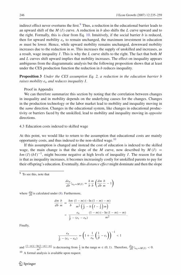
indirect effect never overturns the first.9 Thus, a reduction in the educational barrier leads toan upward shift of the M (I ) curve. A reduction in b also shifts the L curve upward and tothe right. Formally, this is clear from Eq. 10. Intuitively, if the social barrier b is reduced,then for upward mobility en to remain unchanged, the maximum investment in educationm must be lower. Hence, while upward mobility remains unchanged, downward mobilityincreases due to the reduction in m. This increases the supply of unskilled and increases, asa result, wage inequality I . This is why the L curve shifts to the right. The fact that both Mand L curves shift upward implies that mobility increases. The effect on inequality appearsambiguous from the diagrammatic analysis but the following proposition shows that at leastunder the CES production function the reduction in b reduces inequality.

Proposition 3 Under the CES assumption Eq. 2, a reduction in the education barrier braises mobility en and reduces inequality I .

Proof in AppendixWe can therefore summarize this section by noting that the correlation between changes

in inequality and in mobility depends on the underlying causes for the changes. Changesin the production technology or the labor market lead to mobility and inequality moving inthe same direction. Changes in the educational system, like changes in educational produc-tivity or barriers faced by the unskilled, lead to mobility and inequality moving in oppositedirections.

4.3 Education costs indexed to skilled wage

At this point, we would like to return to the assumption that educational costs are mainlyopportunity costs, and thus indexed to the non-skilled wage.10

If this assumption is changed and instead the cost of education is indexed to the skilledwage, the main change is that the slope of the M curve, now described by M (I ) =hm (I ) (bI )−1, might become negative at high levels of inequality I . The reason for thatis that as inequality increases, it becomes increasingly costly for unskilled parents to pay fortheir offspring’s education. Eventually, this distance effect might dominate and then the slope

9 To see this, note that

den

db|en=M(I ) = h

b

m

b

(dm

db

b

m− 1

)

where dmdb is calculated under (8). Furthermore,

dm

db

b

m= hm

b

(1 − m) (−ln (1 − m) − m)

m2(

1β − h

(I − 1

b

)m

)

<en

1β − (es − en)

(1 − m) (− ln (1 − m) − m)

m2 .

Finally,

en1β

− (es − en)=

(1 + 1

en

(1

β− es

))−1< 1

and (1−m)(−ln(1−m)−m)

m2 is decreasing from 12 in the range m ∈ (0, 1) . Therefore, den

db |en=M(I ) < 0.10 A formal analysis is available upon request.

123

J Econ Growth (2007) 12:235–259 247

of the M becomes negative. The conclusion, however, is that the model behaves in a fairlysimilar way under this alternative assumption. The main difference is that at very high levelsof inequality a skill-biased technical change might lead to a reduction of mobility insteadof higher mobility. But we should note that this case appears less plausible for developedeconomies, requiring, in particular, that the level of inequality at which the curve M changesslope is smaller than Imax.

5 Public subsidies to education

This section introduces public support to education. This support can be partial, so that someeducation costs are still privately financed. Our assumption in this section therefore differsfrom those in Glomm and Ravikumar (1992), where public education rules out private expen-ditures on education. In our model public education helps parents increase the probability oftheir children to become skilled by lowering the private cost of schooling. We assume thatpublic education is financed by a proportional tax on income.

Intuitively, one may think that public education should lead to higher mobility and lowerinequality. Public education enables more children of unskilled to go to school, thus raisingupward mobility. It also increases the number of skilled workers and reduces the number ofunskilled, thus lowering inequality. Indeed, these are usually the declared goals of increasesin public education. However, the analysis should take account of other secondary effects,which might reduce these primary effects, and might even harm the declared goals. In orderto assess these opposing effects we turn to a formal analysis of public subsidies to education,which helps us examine these issues within a general equilibrium framework.

Let p be a proportional subsidy to education, paid by a proportional income tax T . Tosimplify calculation we assume that educational spending is tax-deductible. Hence, a parentthat spends a share m of gross income on education consumes (1 − T )(1 − m)w and getshm/(1 − p) units of education if unskilled and hm I/(1 − p) units of education if skilled.Consequently,

en = mh

b (1 − p)

es = mhI

1 − p= enbI,

and, as in the case of changes in h, the L (I ) curve is unaffected by changes in p and T .Note that public subsidies to education benefit skilled parents by more than unskilled in

the sense that ∂es∂p > ∂en

∂p , both because they use education better, provided b > 1, and sincethey have a higher income. This point has been made by Fernandez and Rogerson (1995).However, we have an additional indirect effect through wage inequality. Public educationincreases the supply of skill, which reduces I and thus reduces the difference es − en . Weshow in a numerical example below that it is perfectly possible that the indirect effect domi-nates the direct effect and that despite the double handicap of unskilled parents they increaseeducation attainment by more than skilled parents in the long-run.

To analyze the long-run effects of educational subsidies, we start by analyzing the incen-tives to invest in education. First, note that since the utility loss of taxes is additive, givenby ln (1 − T ), regardless of income and the share spent on education, Eq. 3 is unaffected.11

straightforward calculation yields that (7) now becomes

11 Clearly, a progressive tax system affects educational incentives directly.

123

248 J Econ Growth (2007) 12:235–259

Fig. 5 Welfare as a function ofthe subsidy rate p

1.2

2.2

3.2

4.2

5.2

6.2

0.0

Vn

Vs

VN n VS+ s

erafleW

2.0 4.0 6.0 8.0 0.1

p

Vs − Vn = ln I + (I − 1

b

) h1−p (− (1 − m) ln (1 − m) − m)

1 − β mh1−p

(I − 1

b

) . (11)

An increase in p thus raises the gains from education and its effect is isomorphic to anincrease in h, the productivity of education.

We therefore conclude that inequality falls and upward mobility rises with p. This resultshows that the effect of public education on mobility and inequality is similar to the effectsof the other changes in the educational sector, which are analyzed in Sect. 4.2.

We next briefly discuss some welfare aspects of public education. Specifically, we exam-ine who prefers more subsidies to education, the skilled or the unskilled. On the one hand theunskilled gain more from the subsidy, since it reduces inequality by raising their wage andsince it increases mobility and thus increases their children’s chance to escape from poverty.On the other hand, the skilled can use the public subsidy to education better, since they facea lower barrier to education.

In Fig. 5 we plot the welfare of skilled and unskilled as measured by Vs and Vn , respec-tively, against p. In addition, we also plot aggregate welfare, i.e., N Vn + SVs . We use thesame parameters as above.12

In Fig. 5 we see that Vs is monotonically decreasing in p, while the opposite is true forVn . Public education affects welfare via its effect on inequality and mobility and via the taxcost. The effect of inequality is positive for the unskilled, since their wage rises and negativefor the skilled since their wage declines. The effect through mobility is positive for both,since public education reduces the chance that the child will become unskilled. In Fig. 5 wesee that for the skilled, the inequality effect dominates the mobility effect and they prefer toreduce public education as much as possible. The unskilled gain from public education boththrough inequality and through mobility and despite the fact that they are less likely to getthe subsidy since fewer of their children get educated they prefer to have as much subsidy aspossible.

Figure 5 also shows that average welfare is maximized by a positive subsidy rate. Thesocial optimal subsidy of education is p = 0.751, which is financed by a proportional tax

12 The budget constraint of the government is T = p(

e2s +(1−es )ben

)

2h(n+I )−(1−p)(

e2s +(1−es )ben

) . Proof and code to solve

for the utility levels numerically are available upon request.

123

J Econ Growth (2007) 12:235–259 249

Fig. 6 Mobility vs. inequality

KU

dnalniFadanaCewS

SU

ynamreG

roN

7,0

27,0

47,0

67,0

87,0

8,0

28,0

48,0

68,0

88,0

081071061051041031

pagegawyraitreT

roNewS

reG

KU

SU7,0

27,0

47,0

67,0

87,0

8,0

28,0

48,0

68,0

88,0

8,16,14,12,118,06,0

ytilauqeniegaw01/09

Mo

bil

ity

Mo

bil

ity

of 3.87%. Interestingly these figures are not far from observed values.13 The effect of thissubsidy is to increase upward mobility from en = 0.393 to 0.557. Also es increases, but byless, from es = 0.672 to 0.713. Therefore, the difference in educational attainment, es − en

falls from 0.279 to 0.156, i.e., it is almost cut in half. The changes in es and en increasethe supply of skilled, causing wage inequality to fall from 1.554 to 1.165 and the wage ofunskilled to increase by 21.4%.

The finding that unskilled and skilled have opposing views on public subsidies remainsalso if the barrier to education is much higher. Setting b = 3, for example, implies that mobil-ity, with and without subsidies, is very low. But, nevertheless, the unskilled still prefer 100%subsidies while the skilled still prefer none. Interestingly, the welfare maximizing level ofsubsidies is almost the same as in the low barrier case, it is p = 0.760. The subsidy increasesen from 0.170 to 0.246 and es from 0.843 to 0.870. Also in this case es − en falls, now from0.673 to 0.624. Inequality falls from 1.649 to 1.181 and the wage of unskilled increases by24.9%.

13 The average share of public education in total education costs in OECD countries is 0.884 and the averagepublic education costs as a share of GDP in these countries is 4.96%. Source: OECD in Figures—2005 Edition.Table “Education expenditures”.

123

250 J Econ Growth (2007) 12:235–259

6 Empirical implications

A main message of our theoretical model is that features of the educational system tend togenerate a negative association between inequality and mobility, while features of the labormarket tend to generate a positive association between them. As a result we can use observa-tions on wage inequality and intergenerational mobility in order to learn which underlyingfactors caused them. In this section we review some international comparisons of inequalityand mobility and show that their correlations are in line with the predictions of the model.Measuring wage inequality, e.g., the ratio of skilled to unskilled wages is relatively sim-ple, though the definition of skill might differ across countries. Measuring intergenerationalmobility is more difficult due to lack of sufficient data that go back to past generations. Asa result not many studies have produced internationally comparable measures. One of thesefew studies is Blanden et al. (2005), extending work by Björklund et al. (2002). They providemeasures of mobility, based on intergenerational correlation of income between fathers andsons, for UK, Canada, Denmark, Finland, Norway, Sweden, US and West Germany. Theyfind that Canada and the Nordic countries have relatively high degrees of mobility, Britainand the US have substantially lower mobility, while Germany is an intermediate case. InFig. 6 we plot the reported levels of mobility, measured as 1 minus the intergenerationalpartial correlation coefficient, against measures of wage inequality. In the upper panel, weuse the college education wage gap, taken from the “OECD Education at a glance 2002”. Inthe lower panel, we instead use the log wage difference between the 90th and the 10th wagedecile as reported by Blau and Kahn (1996).14 As we see, the general pattern here is a negativerelation between inequality and mobility. This is largely driven by the difference between,on the one hand, the US and UK, with high inequality and low mobility and on the other, thenorthern European countries and Canada, where inequality is low and mobility is high. Thispattern remains also if other measures of inequality reported in Blau and Kahn (1996) areused. For differences within the group of European countries and Canada, however, such anegative relation is not clearly visible, an observation we will return to below.

Applying our model to the correlations shown in the two graphs leads to a clear conclu-sion. The main difference between the US and UK and the Northern European countriesand Canada lies in the area of education. Despite other possible differences like wage com-pression in Europe, emphasized by Blau and Kahn (1996) and further discussed below, ourinterpretation is that differences in the educational systems must play a more prominent role,given the observed differences in mobility and inequality. There is support in the data for thisinterpretation. In Canada and in the Scandinavian countries, government subsidies to highereducation are substantially higher than in the US and the UK. In Table 1, we report publicspending on tertiary education. The average public spending in Canada and the Scandinaviancountries is almost twice as high as in the UK and the US (2.03% vs. 1.17%) and evenhigher relative to the Mediterranean countries, which we will return to below.15 We alsonote that public expenditures on tertiary education are low in Germany, despite a fairly lowlevel of inequality and a fairly high level of mobility, a fact less easy to explain with ourmodel. However, the fact that the German educational system stands out by relying heav-ily on apprenticeships makes Germany a special case. More than half the cohort of youngindividuals participate in the apprenticeships system including also a substantial share ofindividuals that later get a tertiary education (the “double qualification strategy”), see Ryan

14 Canada and Finland are not included in the data from Blau and Kahn.15 The Scandinavian countries and Canada also spend a larger share of GDP on education below the tertiarylevel, although this is arguably less relevant in the perspective of our model.

123

J Econ Growth (2007) 12:235–259 251

Table 1 Public spending ontertiary education

Source: OECD.stat webpage(http://stats.oecd.org/wbos/)

Average share of GDP 1997–2003 (%)

Norway 1.96

Sweden 2.04

Canada 1.73

Finland 2.02

Denmark 2.38

Germany 1.11

UK 0.96

US 1.38

Italy 0.78

Spain 0.93

Portugal 0.98

Ireland 1.41

Greece 0.85

(2001). A possible interpretation is that the German society as a whole spends a substantialamount of resources on education of high quality provided on an equal opportunity basis,despite a relatively small amount of subsidies channeled directly via the public budget.

We next turn to another group of countries, mainly from Southern Europe. Measures ofmobility for these countries are scarce, but recently Comi (2003) used the European Com-munity Household panel to derive such measures. Despite some problems with this dataset,in particular that sons’ earnings are measured at a rather early age, it has the clear advantagethat the data are collected in a similar way across all countries. The findings of Comi are thatthe Mediterranean countries, Portugal and Ireland have a relatively low degree of intergener-ational mobility. Comi (2003) finds no systematic evidence that the low degree of mobility inthese countries is correlated with the educational wage premia. Hence, mobility in SouthernEurope is lower than in Northern Europe, while inequality is quite similar in the two regions.Such a cross-country difference is not along the diagonal in the mobility/inequality diagramand thus requires more than one difference between the two groups of countries. One ofthe differences between Northern and Southern Europe is that the former spend much morepublic resources on higher education, as seen in Table 1. By itself, this would lead to highermobility in the north, but also lower inequality. We observe the former, but not the latter.We argue that the remaining difference is that wage compression is much more important inSouthern Europe than in Northern.

Wage compression, i.e., that wages differ less than individual productivities, is obviouslyan impossibility when labor and product markets are perfect. However, perfect markets,particularly in Europe, is not a good description of reality. Minimum wages, collective bar-gaining, employment protection legislation, search frictions and legal and other entry barriersare some features of European labor and product markets that create the possibility that wagesdeviate from marginal productivities. Measuring cross-country differences in wage compres-sion is not a simple task and we cannot claim that the evidence is completely conclusive.However, evidence supporting the idea that wage compression is more important in Southernthan in Northern Europe does exist. Mourre (2005) uses the European Unions Structure ofEarnings Survey 2002. Using a standard CES production function, it is shown that a wage

123

252 J Econ Growth (2007) 12:235–259

compression coefficient can be identified by separately estimating a standard labor demandequation and an equation for the relative labor demand as a function of relative wages. Thefinding is that wage compression is large in EU as a whole—relative wages are compressedby between a fifth and a quarter. More importantly, while strong and significant evidence forwage compression is found for continental and Southern Europe, no significant wage com-pression is found for northern EU countries (Denmark, Finland, Sweden and the Netherlands)nor for the Anglo-Saxon countries (Ireland and the UK). This result is perhaps surprisinggiven the long history of strong unions and centralized bargaining in Scandinavia. It shouldbe noted, however, that the so called “solidaric wage policy” pursued by Scandinavian laborunions aimed at reducing horizontal rather than vertical wage differences (see e.g., Agell andLommerud 1993). The idea was that by demanding “equal pay for equal jobs”, structuralchange, i.e., an expansion/contraction of sectors/firms with high/low productivity, could bespeeded up. To the extent that this policy was successful, it would create wage compressionbetween individuals with similar characteristics, i.e., reduce the variance of the wage residual,rather than compressing the college premium or other measures of vertical wage inequality.Another observation, consistent with this, is that the incidence of long-term unemploymentis much higher in Southern than in Northern Europe.16

These empirical findings mean that the countries in Northern Europe differ from the coun-tries in Southern Europe in two main aspects relevant to our theory. Northern Europe hasmore public education than the South, and has less wage compression in the labor market.The first difference should lead to higher mobility and more equality in Northern Europe.The second difference should lead to less equality but more mobility in Northern Europe.Indeed, the data show that Northern Europe is much more mobile than SouthernEurope. Since the two differences affect inequality in two opposite ways it is not surprisingthat in reality inequality is found to be similar in the North and the South of Europe. Hence,this relationship also fits our model fairly well.

Checchi et al. (1999) provide further empirical evidence to this conclusion. They comparemobility and inequality in Italy and in the US and find that while mobility in Italy is lowerthan in the US, also inequality is much lower than in the US. According to our model, thepositive correlation between mobility and inequality when comparing Italy and the US, pointsto differences in the labor market. As discussed above, the evidence in Mourre (2005) is thatwage compression is high in Southern Europe. Furthermore, comparing the US and Europe,Blau and Kahn (1996, 2002), show that labor market regulation created significant wagecompression in European countries compared to the US and the UK. Blanchard and Wolfers(2000) have also shown that the higher unemployment in Europe is due to labor regulations,like generous unemployment benefits, high minimum wages, high firing costs, and more.Alesina, Glaeser and Sacerdote (2005) have shown that such labor market regulations havereduced hours worked in Europe relative to the US. More specifically, Erikson and Ichino(1994) document an “extreme compression” of wages in Italy during the 1970s.

Another international comparison of intergenerational mobility appears in Dahan andGaviria (2001). They study 16 Latin American countries and compare them to the US. Inorder to overcome data limitations this paper develops an interesting measure to mobilitywhich happens to be close in spirit to this paper. They measure it by sibling correlations ofsuccess and failure in the schooling system. Dahan and Gaviria find that within the LatinAmerican countries and even more so relative to the US, inequality and mobility are nega-tively correlated. Thus, the average Gini coefficient in the Latin American countries is .51

16 The average share of unemployed with an unemployment duration over a year in the years 2000–2006 was19% in Scandinavia, 10% in the US, 24% in the UK, but as large as 57% in Italy. Source: OECD.stat webpage.(http://stats.oecd.org/wbos/).

123

J Econ Growth (2007) 12:235–259 253

while it is .379 in the US. Mobility (1−sibling coefficient) is .505 in the Latin Americancountries while it is equal to .797 in the US. This negative correlation points at differences inthe education system between the two regions. Indeed, comparing the public expenditures’share of GDP relative to the percentage of children in the two regions (which is a proxy forwhat is called p in the model) we get that the public support to education in the US is muchlarger. This figure is .248 in the US, while it is only .109 in the 16 Latin American countries,namely higher by a factor of two and a half. Hence, higher public support to education in theUS relative to Latin America comes with higher mobility and lower inequality, as the modelpredicts.

We conclude this section with a few observations on changes in mobility and inequalityover time. Empirical comparisons of mobility over time are very rare, as mobility measure-ments are rather new and it is hard to find data for past generations. One exception is Lambertet al. (2007), who use a host of data sets on mobility. Most of these data sets are fairly recent,from the Post War period. But they also add a unique historical data set from the CambridgeFamily History Study. This data set consists of people who traced their family history backin time over a long period of time, of more than two centuries. This is of course not a sample,but it supplies significant information on the dynamics of mobility in Britain. As mentionedabove, the authors use more data sets for recent periods. The way they measure mobility isoccupational, which fits the spirit of our paper well. They measure occupational correlationbetween father and child. The pattern the study finds, as presented in Fig. 1 in that paper, isthat mobility in Britain has been on a steady but very slow and gradual rise in the last twocenturies. Interestingly, since the 1970s mobility began to rise much more rapidly. This resultis interesting since 1972 is an important year in the history of public education in the UK. Inthat year compulsory education was extended to the age of 16 from an age of 12. Althoughthere was a mechanism that enabled extension for bright students to secondary school since1902, but it was not until 1972 that this extension became effective for all. The coincidencebetween this change and the sharp rise in mobility adds another empirical support to ourmodel.

Another example of measuring changes in mobility over time is supplied by Güell et al.(2007), who measure intergenerational mobility in Catalonia by studying surnames. Theycompare people above and below the age of fifty and find that mobility in the current genera-tion is lower than in the previous generation. Interestingly the skilled to unskilled wage ratiofor the older generation were close to 2, while for the younger generation it is 1.56. Thusboth mobility and inequality went down, pointing in the direction of changes in labor marketinstitutions. Indeed, Spain went through a significant change thirty years ago with the deathof Franco. While before his death labor unions were not allowed and labor markets were notregulated, after his death labor unions regained much importance and labor market policiesbecame more similar to other Southern European countries. Hence, Spain went through amajor increase in wage compression. The expected effect of such a change on inequality andmobility according to our model is indeed in line with the results of Güell et al. (2007).

Another phenomenon that our analysis can shed light on is the rise of wage inequalityin the US in recent decades. The main explanation to this increase has been skill-biasedtechnical change, but there have been other explanations as well. Our model claims that ifthis widening of the wage gap is a result of SBTC, then it should be accompanied with anincrease in intergenerational mobility as well. Indeed Mayer and Lopoo (2001) find evidencein PSID data that intergenerational mobility is higher for individuals born after 1953. Thus,although a small sample size and the difficulty to measure lifetime income make this findingsomewhat preliminary, it clearly supports our model’s predictions. A skill biased technicalchange increases both inequality and mobility.

123

254 J Econ Growth (2007) 12:235–259

7 Conclusions

This paper presents a simple theoretical model that analyzes the joint determination of incomeinequality, skill distribution and intergenerational mobility. Its main focus is on the expectedcorrelation between inequality and mobility. Empirical studies have shown that this correla-tion across countries can be either positive or negative. Our paper gives a simple explanationto these findings. We show that the correlation between inequality and mobility is positiveif the underlying differences are in the production sector, while the correlation is negativeif the underlying changes are in the education sector. In the empirical section of the paper,we review results supporting the predictions of our model and we therefore believe it helpsin understanding observed differences in inequality across countries, and also over time in asingle country.

Our model can be used to examine additional economic, social and cultural variables.For example, the analysis of the case of missing information in the appendix shows, thatcountries, in which parents are more dominant within the family, tend to have less education,less mobility and higher inequality. We believe that the framework presented here can befurther extended in many other interesting directions.

Finally, we have shown that public subsidies to education may be particularly beneficialfor unskilled individuals. It is tempting to interpret this result as saying that unskilled votersshould be expected to vote in favor of educational subsidies. However, it may be premature todraw such a conclusion. First, we analyze steady states and the inequality reducing effect ofeducational subsides occurs with a substantial lag since it takes time for the relative suppliesof skilled and non-skilled to change after an educational reform. Second, we have analyzedthe consequences of a permanent change in the subsidy rate, while political decisions maybe better modeled as taken without commitment. We leave the study of the dynamic politi-cal determination of educational subsidies in a model with endogenous wage formation forfuture work.

Acknowledgments We thank Omer Moav and Fabrizio Zilibotti for very useful comments on previous drafts.We also thank the referees and the editor of this journal for important suggestions and criticisms. JVRM thanksthe financial support of the Spanish Ministry of Science and Education (project SEJ2004-06877).

Appendix

Appendix 1: Proofs

Proof of proposition 1

We can rewrite (8) as:(

h

(I − 1

b

)− 1

β

)(−ln (1 − m)) + ln I = h

(I − 1

b

)m (A.1)

The RHS of (A.1) is a linear increasing function of m while the LHS is going from ln Ito ∞ (or − ∞) and is increasing and convex (decreasing and concave) if h

(I − 1

b

) − 1β

islarger (smaller) than zero. Hence, there can be at most two solutions to (A.1). We show belowthat the smallest solution, denoted m (I ), is the relevant one since the larger implies es > 1.

We begin the analysis with I = 1. In this case m = 0 is a solution. If h(I − 1

b

) − 1β

≤ 0,a unique solution clearly exists for any I ≥ 1.

123

J Econ Growth (2007) 12:235–259 255

Now consider the alternative case, h(I − 1

b

) − 1β

> 0. Note that the LHS has a strictlysmaller derivative with respect to m at m = 0. Therefore, continuity ensures that a solutionremains for I > 1 in a neighborhood of 1. For a sufficiently high level of inequality nosolution exists. The maximum level of inequality for which a solution exists is I ∗ where thesolution m∗ occurs at the tangency of the LHS and the RHS, namely at

m∗ = m(I ∗) = 1

βh(I ∗ − 1

b

) .

Hence, for I < I ∗, at least one solution exists, that is m (I ) exists in the range I ∈ [1, I ∗].

Next, we show that the smallest solution m (I ) is the only solution to (A.1) such that es ≤ 1.To see this, note that if there are two intersection points to the two sides of (A.1), then inbetween them, there is a point m p , where the two curves have the same slope, given by

m p = 1

βh(I − 1

b

) ,

where we note that m p < 1 when h(I − 1

b

) − 1β

> 0. If there were two solutions to (A.1),then in one m > m p . Then

es = mhI > m phI = I

β(I − 1

b

) ≥ 1.

We next analyze the slope of the function m(I ). First, note that the LHS (A.1) must cutthe RHS from above at m = m (I ). Second, a higher I raises both the LHS and the RHSof (A.1). But since −ln (1 − m) > m, the LHS rises by more than the RHS. Therefore, anincrease in I must lead to higher m, i.e., m′ (I ) > 0.

Finally, implicitly define Imax from

m (Imax) hImax = 1,

i.e., as the highest level of inequality such that es is no larger than unity. To conclude theproof, we must show that Imax ≤ I ∗. Now, at I ∗, we have

m(I ∗) hI ∗ = I ∗

β(I ∗ − 1

b

) > 1.

Since m (I ) hI is increasing in I, I ∗ > Imax

Proof of proposition 3

Using, the definition of es and en , solving for m, and substituting in (8), yields

X ≡ −ln I −(

h

(I − 1

b

)− 1

β

)(−ln

(1 − b

h (I σ + I b)

))

+ h

(I − 1

b

) (b

h (I σ + I b)

)= 0.

From this we can calculate

d I

db= −

d Xdbd Xd I

123

256 J Econ Growth (2007) 12:235–259

where

d X

d I= −1

I+ h

(ln

(1 − b

h (I σ + I b)

))+

(h

(I − 1

b

)− 1

β

) b(I σ−1σ+b

)h(I σ +I b)2

(1 − bh(I σ +I b)

)

+ h

(b

h (I σ + I b)

)− h

(I − 1

b

)b

(I σ−1σ + b

)

h (I σ + I b)2

= hm − 1

I− h (−ln(1 − m)) −

(m

1 − m

(1

β− hm

(I − 1

b

))) (I σ−1σ + b

)

I(I σ−1 + b

)

= −1 − es

I− h (−ln(1 − m)) −

(m

1 − m

(1

β− (es − en)

)) (I σ−1σ + b

)

I(I σ−1 + b

) < 0

and

d X

db= h

b2

(ln

(1 − b

h (I σ + I b)

))−

(h

(I − 1

b

)− 1

β

) I σ

h(I σ +I b)2

1 − bh(I σ +I b)

+ h

b2

(b

h (I σ + I b)

)+ h

(I − 1

b

)I σ

h (I σ + I b)2

= h

b2 (ln(1 − m)) + h

b2 m + 1

1 − m

m

b

(1

β− (es − en)

)I σ

I σ + I b

= h

b2 (1 − m)

((1 − m) ln(1 − m) + m + m2

(1

β− (es − en)

)I σ

)>

= h

b2 (1 − m)((1 − m) ln(1 − m) + m) > 0 ∀m > 0

To see the latter, note that

limm→0

((1 − m) ln(1 − m) + m) = 0

and

d ((1 − m) ln(1 − m) + m)

dm= − ln (1 − m) > 0.

Appendix 2: Unknown inaptitude

In the benchmark model we assume that inaptitude of a child is already known when educa-tion decision is made. In this appendix we explore the possibility that inaptitude is unknownat the time of this decision. While the main results of the paper still hold, one important newissue emerges. Under missing information parents and children bargain over the amount ofinvestment in education, and it therefore depends on their relative bargaining strengths. Thisopens a discussion on the effect of differences in social and cultural norms on inequality andmobility.

Assume that the amount of education is decided before inaptitude is known. When edu-cation begins, the child immediately observes whether she can finish school or not, namelywhether e is below or above the amount of education purchased. If she can, she remains inschool, and if not she leaves school and the parents get their money back. Note that underthese informational assumptions, the offspring can bargain with the parent on the size of

123

J Econ Growth (2007) 12:235–259 257

investment in education, threatening not to go to school if the amount is not high enough.The underlying conflict reflects the different interests of parents and children. While the latteralways want to have more education, to raise probability of success, parents share this desire,but also care about own consumption. This conflict of interests is resolved in bargaining. Weassume that parent and offspring use a simple form of asymmetric Nash bargaining.

The expected utility of parents at time of bargaining is:

ln w j + βVn + e j[ln

(1 − m j

) + β (Vs − Vn)]

where j = s if skilled and n if unskilled. The threshold levels are: es = ms I h and en =mnh/b.

The expected utility of children to parents of type j is:

Vn + e j (Vs − Vn)

The threat points are ln w j +βVn and Vn for parent and child respectively, and if the relativebargaining power of parents is denoted by q , the logarithm of the asymmetric Nash-productis

ln e j + q ln[ln

(1 − m j

) + β (Vs − Vn)] + (1 − q) ln (Vs − Vn).

Substituting the threshold levels and maximizing yields that skilled and unskilled spendthe same share of income m on education, which is determined by:

β (Vs − Vn) + qm

1 − m− ln (1 − m). (A.2)

We see that a higher bargaining power to parents q , reduces the share of income that goesto education m. While (A.2) is the new incentive curve in this extension, the gains curve is thesame as in the benchmark model. Calculating the two relations together yields the functionm

− ln (1 − m)

β+ qm

1 − m

[1

β− h

(I − 1

b

)m

]

= ln (I ) + h

(I − 1

b

)[−ln (1 − m) − m]. (12)

Note that (12) is similar to the equilibrium condition (8), except for the element thatdepends on q . The other equilibrium conditions are derived as in the benchmark model.Clearly, the main results of the paper remain intact. The only novelty here is the new vari-able q , the bargaining power of parents. As the LHS of (12) increases with q , it leads to adownward shift of m and of the M curve, while the L curve remains unchanged. Intuitively,when parents have more bargaining power over their children, they consume more and payless for their education. Hence, upward mobility decreases and inequality increases. Thus,the social power of parents within the family can be another potential explanation for highinequality and low mobility.

References

Aghion, P., & Bolton, P. (1997). A theory of trickle-down growth and development. The Review of EconomicStudies, 64(2), 151–172.

Alesina, A., Glaeser, E., & Sacerdote, B. (2005). Work and leisure in the U.S. and Europe: Why so different?NBER Macroeconomics Annual, 20, 1–64.

123

258 J Econ Growth (2007) 12:235–259

Alesina, A., & Rodrik, D. (1994). Distributive politics and economic growth. The Quarterly Journal of Eco-nomics, 109(2), 465–490.

Baland, J. M., & Robinson, J. A. (2000). Is child labor inefficient? Journal of Political Economy, 108(4),663–679.

Banerjee, A. V., & Newman, A. F. (1993). Occupational choice and the process of development. Journal ofPolitical Economy, 101(2), 274–298.

Barro, R. J. (2000). Inequality and growth in a panel of countries. Journal of Economic Growth, 5(1), 5–32.Benabou, R. (2001). Social mobility and the demand for redistribution: The poum hypothesis. The Quarterly

Journal of Economics, 116(2), 447–487.Benabou, R. (2002). Tax and education policy in a heterogeneous-agent economy: What levels of redistribution

maximize growth and efficiency? Econometrica, 70(2), 481–517.Björklund, A., Eriksson, T., Jantti, M., Raaum, O., & Osterbacka, E. (2002). Brother correlations in earnings

in Demark, Finland, Norway and Sweden compared to the United States. Journal of Population Economics,15(4), 757–772.

Blanchard, O. J., & Wolfers, J. (2000). The role of shocks and institutions in the rise of european unemployment:The aggregate evidence. Economic Journal 110, 1–33.

Blanden, J., Gregg, P., & Machin, S. (2005). Intergenerational mobility in Europe and North America—areport for the Sutton Trust. Centre for Economic Performance, London School of Economics.

Blau, F., & Kahn, L. M. (1996). International differences in male wage inequality: Institutions and marketforces. Journal of Political Economy, 104(4), 791–837.

Blau, F., & Kahn, L. (2002). At home and abroad: U.S. labor markets in international perspective. New York,NY: Russell Sage.

Checchi, D., Ichino, A., & Rustichini, A. (1999). More equal but less mobile? Education financing and inter-generational mobility in Italy and in the US. Journal of Public Economics, 74(3), 351–393.

Comi, S. (2003). Intergenerational mobility in Europe: Evidence from ECHP. Mimeo, Univerista degli studidi Milano.

Cooper, S., Durlauf, S. N., & Johnson, P. A. (1993). On the evolution of economic status across generations.American Statistical Association Proceedings of Business and Economics, 83, 50–58.

Dahan, M., & Gaviria, A. (2001). Sibling correlations and intergenerational mobility in Latin America. Eco-nomic Development & Cultural Change, 49(3), 537–554.

Doepke, M., & Zilibotti, F. (2005). The macroeconomics of child labor regulation. American Economic Review,95, 1492–1524.

Durlauf, S. N. (1996). A theory of persistent income inequality. Journal of Economic Growth, 1(1), 75–93.Erikson, C. L., Ichino, A. (1994). Wage differentials in Italy: Market forces, institutions, and inflation. NBER

Working Paper No. 4922, 1994.Fender, J., & Wang, P. (2003). Educational policy in a credit constrained economy with skill heterogeneity.

International Economic Review, 44, 939–964.Fernandez, R., & Rogerson, R. (1995). On the political economy of education subsidies. Review of Economic

Studies, 62(2), 249–262.Fernandez, R., & Rogerson, R. (1998). Public education and income distribution: A dynamic quantitative

evaluation of education-finance reform. American Economic Review, 88(4), 813–833.Galor, O., & Zeira, J. (1993). Income distribution and macroeconomics. The Review of Economic Studies,

60(1), 35–52.Galor, O., & Tsiddon, D. (1997). Technological progress, mobility, and economic growth. American Economic

Review, 87, 363–382.Glomm, G., & Ravikumar, B. (1992). Public versus private investment in human capital, endogenous growth

and income inequality. Journal of Political Economy, 100(4), 813–834.Güell, M., Rodríguez Mora, J. V., & Telmer, C. (2007). Intergenerational mobility and the informative content

of surnames. CEPR DP 6316.Hassler, J., & Rodríguez Mora, J. V. (2000). Intelligence, social mobility, and growth. American Economic

Review, 90(4), 888–908.Hornstein, A., & Krusell, P. (2003). Implications of the capital-embodiment revolution for directed R&D and

wage inequality. Federal Reserve Bank of Richmond Economic Quarterly, 89(4), 25–50.Lambert, P., Prandy, K., & Bottero, W. (2007). By slow degrees: Two centuries of social reproduction and

mobility in britain. Sociological Research Online, 12(1).Loury, G. C. (1981). Intergenerational transfers and the distribution of earnings. Econometrica, 49(4), 843–

867.Maoz, Y. D., & Moav, O. (1999). Intergenerational mobility and the process of development. Economic

Journal, 109(458), 677–697.

123

J Econ Growth (2007) 12:235–259 259

Mayer, S. E., & Lopoo, L. M. (2001). Has the intergenerational transmission of economic status changed?Mimeo.

Mourre, G. (2005). Wage compression and employment in Europe: First evidence from the structure of earn-ings survey 2002. Economic Papers no. 232, September 2005, European Commission, Directorate-Generalfor Economic and Financial Affairs.

Owen, A. L., & Weil, D. N. (1998). Intergenerational earnings mobility, inequality and growth. Journal ofMonetary Economics, 41(1), 71–104.

Perotti, R. (1996). Growth, income distribution, and democracy: What the data say. Journal of EconomicGrowth, 1(2), 149–187.

Persson, T., & Tabellini, G. Is inequality harmful for growth? American Economic Review, 84(3), 600–621.Ryan, P. (2001). The school-to-work transition: A cross-national perspective. Journal of Economic Literature,

39(1), 34–92.Solon, G. (1999). Intergenerational mobility in the labor market. Handbook of Labor Economics (Vol. 3A).

In O. Ashenfelter & D. Card (Eds.), Handbooks in economics (Vol. 5, pp. 1761–1800). Amsterdam; NewYork and Oxford: Elsevier Science, North-Holland.

Solon, G. (2004). A model of intergenerational mobility variation over time and place. In Corak, M. (Ed.),Generational income mobility in North America and Europe. Cambridge: Cambridge University Press.

123