JOAN ROBINSON WAS ALMOST RIGHT: OUTPUT UNDER THIRD-

DEGREE PRICE DISCRIMINATION

by

Iñaki Aguirre

2009

Working Paper Series: IL. 38/09

Departamento de Fundamentos del Análisis Económico I

Ekonomi Analisiaren Oinarriak I Saila

University of the Basque Country

Joan Robinson Was Almost Right:Output under Third-Degree Price

DiscriminationDecember 2008

Iñaki Aguirre1University of the Basque Country

ABSTRACT

In this paper, we show that in order for third-degree price discriminationto increase total output, the demands of the strong markets should be, asconjectured by Robinson (1933), more concave than the demands of theweak markets. By making the distinction between adjusted concavity of theinverse demand and adjusted concavity of the direct demand, we are ableto state necessary conditions and su¢ cient conditions for third-degree pricediscrimination to increase total output.

Keywords: Third-Degree Price Discrimination, Output, Monopoly, Wel-fare.

JEL Classi�cation: D42, L12, L13.

1I would like to thank Miguel Aramendía, Simon Cowan and Ignacio Palacios-Huertafor helpful comments. Financial support from the Ministerio de Ciencia y Tecnología andFEDER (SEJ2006-05596), and from the Departamento de Educación, Universidades eInvestigación del Gobierno Vasco (IT-223-07) is gratefully acknowledged. Departamentode Fundamentos del Análisis Económico I, Avda. Lehendakari Aguirre 83, 48015-Bilbao,Spain. E-mail: inaki.aguirre@ehu.es. Website: www.ehu.es/iaguirre.

1

1 Introduction

A move from uniform pricing to third-degree price discrimination generatestwo e¤ects: �rst, price discrimination causes a misallocation of goods fromhigh to low value users (in other words, price discrimination is an ine¢ -cient way of distributing output between di¤erent consumers) and, second,price discrimination a¤ects total output.1 Therefore, a necessary conditionfor third-degree price discrimination to increase social welfare is that it in-creases total output.2 As a result, a focal point has been the analysis ofthe e¤ects of price discrimination on output. Since Robinson (1933) manyarticles have addressed this issue, including Leontief (1940), Edwards (1950),Silberberg (1970), Löfgren (1977), Ippolito (1980), Smith and Formby (1981),Formby, Layson and Smith (1983), Schmalensee (1981), Shih, Mai and Liu(1988), Cheung and Wang (1994), Aguirre (2006), Cowan (2007), and Cowanand Vickers (2007), among others.3 The e¤ect of third-degree price discrim-ination on total output is intrinsically related to how the shape of demandsin strong markets (markets where the optimal discriminatory price exceedsthe optimal single price) compares to that in weak markets (where the opti-mal discriminatory prices are lower than the single price). It is known fromPigou (1920) that under linear demands price discrimination does not changeoutput. In the general non-linear case, however, the e¤ect of price discrimi-nation on output may be either positive or negative. It is well known (see,for example, Robinson, 1933, Silberberg, 1970, or Schmalensee, 1981) thatwhen all the strong markets have concave demands whereas the weak mar-kets have convex demands (with at least one market with strict concavityor convexity) then third-degree price discrimination increases output. Whenstrong markets have convex demands and weak markets concave demandsprice discrimination reduces output. In the case in which all the demand

1See, for example, Ippolito (1980), Schmalensee (1981) or Aguirre (2008) for explicitdecompositions of the change in social welfare into these two e¤ects: the misallocatione¤ect and the output e¤ect.

2Schmalensee (1981) proves this conjecture assuming nonlinear demand curves, per-fectly separated markets and constant marginal cost. Varian (1985), Schwartz (1990) andmore recently Bertoletti (2004) generalize the result.

3It is assumed throughout the paper that all markets are served under both pricingregimes, uniform pricing and price discrimination. The possibility that price discriminationopens up new markets (and that may even yield Pareto improvements) was also consideredby Robinson (1933). See, for example, Battalio and Ekelund (1972), Hausman and Mackie-Mason (1988) and Layson (1994) for more recent analysis.

2

curves have similar curvature the answer is more complicated. We completepartially the theorem by Robinson (1933) and show that she was almost rightwhen stated that

�If both (curves) are (strictly) concave or both (strictly) convex it isobvious that the result (the e¤ect on output) must depend upon whether ornot the more elastic demand curve is, in some sense, "more concave" thanthe less elastic demand curve (p. 193).�4

In particular we show that in order for third-degree price discriminationto increase total output the demand in the strong markets should be in somesense more concave than the demand in the weak markets. By making thedistinction between adjusted concavity of the inverse demand (the measureused by Robinson, 1933) and adjusted concavity of the direct demand, weare able to state necessary conditions and su¢ cient conditions for third-degree price discrimination to increase total output. A su¢ cient condition forthird-degree price discrimination to increase total output is that all curves,demands and inverse demands, are more concave in strong markets. Onthe other hand, we show that if demands and inverse demands are less (orequally) concave in the strong markets than in the weak markets then third-degree price discrimination does not increase total output.The paper is organized as follows. Section 2 introduces di¤erent measures

of adjusted concavity of demands and inverse demands and shows how theyare related to each other. In Section 3, we study the e¤ects of third-degreeprice discrimination on total output and we state necessary conditions andsu¢ cient conditions for price discrimination to increase output. In Section4, we arrange previous results in the literature. Finally, Section 5 o¤ersconcluding remarks.

4Robinson (1933) uses the terms concave and convex just in the opposite way to how itwill be used in this paper. We follow the modern convention over concavity and convexity.

3

2 Direct demands, inverse demands and con-cavity

Economists typically use the terms demand and inverse demand interchange-ably. Although this practice is generally irrelevant, when we study di¤erentmarkets the comparison of their degree of concavity may depend cruciallyon whether we consider demands or inverse of demands. Assume that thedemand function in market i = 1; :::; n is given by Di(pi), with D

0i(pi) < 0,

where pi is the price charged in that market and the inverse demand func-tion is pi(qi), with p

0i(qi) < 0, where qi is the quantity sold. We assume

that all curves (demands and inverse demands) are everywhere continuousand di¤erentiable. The elasticity of demand of market i is given by "i(pi) =�D0

i(pi)pi

Di(pi)as a function of the price or, equivalently, "i(qi) = � 1

p0i(qi)

pi(qi)qias

a function of the quantity. We distinguish between the concavity of the directdemand and the concavity of the inverse demand. The (adjusted) concavity

of the direct demand in market i, CDi (pi), is given by CDi (pi) = pi

D00i (pi)

D0i(pi)

, and

the (adjusted) concavity of the inverse demand in market i, CIi (qi), is given

by CIi (qi) = qip00i (qi)

p0i(qi)

. From Robinson (1933) the term CIi (qi) has been referred

to, indistinctly, as adjusted concavity of the demand or adjusted concavity ofthe inverse demand. However, if we accept that pi(qi) represents the inversedemand and Di(pi) the demand function, it seems more reasonable that theconcavity of the inverse demand be measured by CIi (:) and the concavity ofthe demand by CDi (:). In fact, as we show in the next section, this distinctionwill be important when we study the e¤ects of third-degree price discrimina-tion on output. The next lemma states the relation between these measuresof demand concavity.

Lemma 1.(i) CDi (pi) = "i(pi)C

Ii (pi).

(ii) CDi (qi) = "i(qi)CIi (qi).

Proof. By twice di¤erentiating the identities pi � pi(Di(pi)) and qi �Di(pi(qi)) with respect to pi and qi, respectively, we obtain:

CIi (pi) = �D

00

i (pi)Di(pi)

[D0i(pi)]

2;

4

CDi (qi) = �p00

i (qi)pi(qi)

[p0i(qi)]

2:

Therefore, taking into account the de�nition of the elasticity of demandin market i, it is direct to obtain CDi (pi) = "i(pi)C

Ii (pi) and C

Di (qi) =

"i(qi)CIi (qi).

5�

Note that the two measures, CDi and CIi , have the same sign: if demand

is strictly concave/strictly convex/linear then inverse demand is strictly con-cave/strictly convex/linear and viceversa. We assume that any demand (orinverse demand) curve which is strictly concave (or linear or strictly convex)remains so throughout the relevant range. On the other hand, we assume thatthe curves of all the strong (weak) markets have the same general curvature.Put di¤erently, the case where some strong (weak) markets have strictly con-cave demands and some strong (weak) markets have strictly convex demandis ruled out.

3 Analysis

Consider a monopolist selling a good in n perfectly separated markets. Thedemand function in market i is given by Di(pi), where pi is the price chargedin that market and the inverse demand function is pi(qi), where qi is thequantity sold. Unit cost, c, is assumed constant. We shall obtain the changein total output due to third-degree price discrimination by solving �rstly theproblem in prices and then the problem in quantities.

Under price discrimination, the optimal policy for the monopolist is givenby:

Di(pdi ) + (p

di � c)D

0

i(pdi ) = 0 i = 1; :::; n; (1)

where pdi denotes the optimal price in market i (and pro�t functions areassumed strictly concave in the relevant range). The quantity sold in marketi is qdi = Di(p

di ), i = 1; :::; n. The total output under price discrimination is

5See also Cowan (2007) and Cowan and Vickers (2007).

5

Qd =nXi=1

qdi =nXi=1

Di(pdi ). Given �rst order conditions (1), total output can

be expressed as:

Qd =nXi=1

Di(pdi ) = �

nXi=1

(pdi � c)D0

i(pdi ): (2)

Under simple monopoly pricing, pro�ts are maximized by charging all con-sumers a common price p0 such that:

nXi=1

Di( p0) + ( p0 � c)

nXi=1

D0

i( p0) = 0: (3)

The quantity sold in market i is q0i = Di(p0), i = 1; :::; n. The total out-

put under uniform pricing is Q0 =nXi=1

q0i =

nXi=1

Di( p0). Given �rst order

condition (3), total output can be expressed as:

Q0 =nXi=1

Di(p0) = �

nXi=1

(p0 � c)D0

i(p0): (4)

Given conditions (2) and (4) the change in total output, �Q = Qd �Q0, isgiven by:

�Q = :Qd �Q0 = �nXi=1

(pdi � c)D0

i(pdi ) +

nXi=1

(p0 � c)D0

i(p0). (5)

We can write condition (5) as:

�Q = �nXi=1

(Z pdi

p0dh(pi � c)D

0

i(pi)i). (6)

Therefore, we get:

6

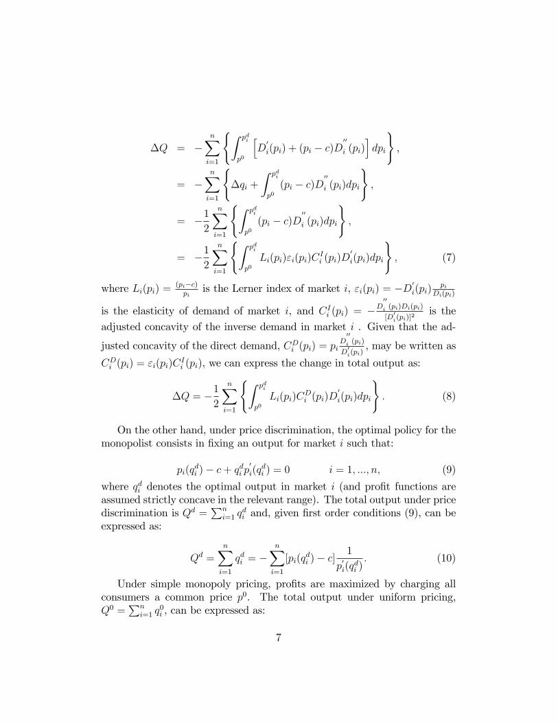
�Q = �nXi=1

(Z pdi

p0

hD

0

i(pi) + (pi � c)D00

i (pi)idpi

),

= �nXi=1

(�qi +

Z pdi

p0(pi � c)D

00

i (pi)dpi

);

= �12

nXi=1

(Z pdi

p0(pi � c)D

00

i (pi)dpi

);

= �12

nXi=1

(Z pdi

p0Li(pi)"i(pi)C

Ii (pi)D

0

i(pi)dpi

); (7)

where Li(pi) =(pi�c)pi

is the Lerner index of market i, "i(pi) = �D0i(pi)

piDi(pi)

is the elasticity of demand of market i, and CIi (pi) = �D00i (pi)Di(pi)

[D0i(pi)]

2is the

adjusted concavity of the inverse demand in market i . Given that the ad-

justed concavity of the direct demand, CDi (pi) = piD00i (pi)

D0i(pi)

, may be written as

CDi (pi) = "i(pi)CIi (pi), we can express the change in total output as:

�Q = �12

nXi=1

(Z pdi

p0Li(pi)C

Di (pi)D

0

i(pi)dpi

): (8)

On the other hand, under price discrimination, the optimal policy for themonopolist consists in �xing an output for market i such that:

pi(qdi )� c+ qdi p

0

i(qdi ) = 0 i = 1; :::; n; (9)

where qdi denotes the optimal output in market i (and pro�t functions areassumed strictly concave in the relevant range). The total output under pricediscrimination is Qd =

Pni=1 q

di and, given �rst order conditions (9), can be

expressed as:

Qd =nXi=1

qdi = �nXi=1

[pi(qdi )� c]

1

p0i(q

di ): (10)

Under simple monopoly pricing, pro�ts are maximized by charging allconsumers a common price p0. The total output under uniform pricing,Q0 =

Pni=1 q

0i , can be expressed as:

7

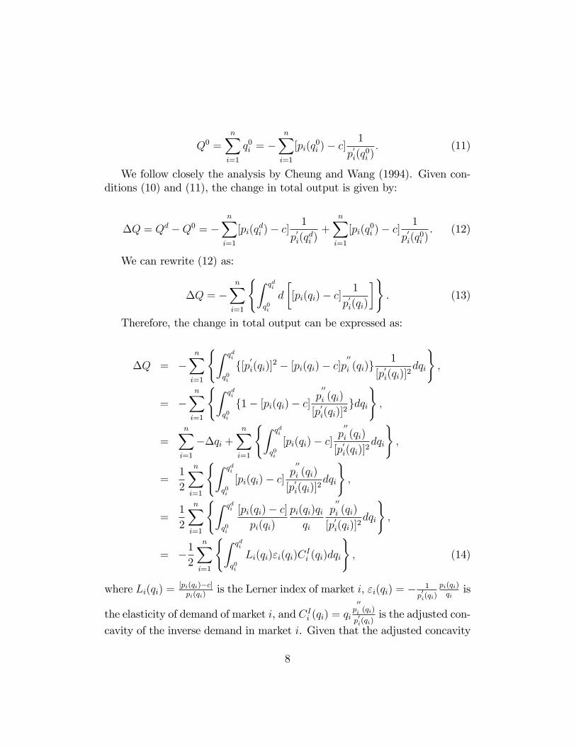
Q0 =

nXi=1

q0i = �nXi=1

[pi(q0i )� c]

1

p0i(q

0i ): (11)

We follow closely the analysis by Cheung and Wang (1994). Given con-ditions (10) and (11), the change in total output is given by:

�Q = Qd �Q0 = �nXi=1

[pi(qdi )� c]

1

p0i(q

di )+

nXi=1

[pi(q0i )� c]

1

p0i(q

0i ). (12)

We can rewrite (12) as:

�Q = �nXi=1

(Z qdi

q0i

d

�[pi(qi)� c]

1

p0i(qi)

�). (13)

Therefore, the change in total output can be expressed as:

�Q = �nXi=1

(Z qdi

q0i

f[p0i(qi)]2 � [pi(qi)� c]p00

i (qi)g1

[p0i(qi)]

2dqi

);

= �nXi=1

(Z qdi

q0i

f1� [pi(qi)� c]p00

i (qi)

[p0i(qi)]

2gdqi

);

=nXi=1

��qi +nXi=1

(Z qdi

q0i

[pi(qi)� c]p00

i (qi)

[p0i(qi)]

2dqi

);

=1

2

nXi=1

(Z qdi

q0i

[pi(qi)� c]p00

i (qi)

[p0i(qi)]

2dqi

);

=1

2

nXi=1

(Z qdi

q0i

[pi(qi)� c]pi(qi)

pi(qi)qiqi

p00

i (qi)

[p0i(qi)]

2dqi

);

= �12

nXi=1

(Z qdi

q0i

Li(qi)"i(qi)CIi (qi)dqi

); (14)

where Li(qi) =[pi(qi)�c]pi(qi)

is the Lerner index of market i, "i(qi) = � 1

p0i(qi)

pi(qi)qi

is

the elasticity of demand of market i, and CIi (qi) = qip00i (qi)

p0i(qi)

is the adjusted con-

cavity of the inverse demand in market i. Given that the adjusted concavity

8

of the direct demand, CDi (qi) = �p00i (qi)pi(qi)

[p0i(qi)]

2, is given byCDi (qi) = "i(qi)C

Ii (qi),

we can express the change in total output as:

�Q = �12

nXi=1

(Z qdi

q0i

Li(qi)CDi (qi)dqi

): (15)

Although we conjecture that the results are more general, following Che-ung and Wang (1994) we restrict our analysis to say that demands in strongmarkets are more (less) concave than demands in weak markets if the min-imum (maximum) value of demand adjusted concavity over the range ofoutput levels between the simple monopoly and discriminatory outputs ineach of the strong markets is greater (lower) than the maximum (minimum)value of demand adjusted concavity over the corresponding ranges of out-put in all of the weak markets. In a similar way, we may de�ne when theinverse demands are more or less concave in strong markets as compared toweak markets. We de�ne these maximum and minimum values of adjustedconcavity as:

CD

s = maxfCDi (qi); qi 2 [qdi ; q0i ]; i 2 Sg = maxfCDi (pi); pi 2 [p0; pdi ]; i 2 Sg;

CD

w = maxfCDi (qi); qi 2 [q0i ; qdi ]; i 2 Wg = maxfCDi (pi); pi 2 [pdi ; p0]; i 2 Wg;

CDs = minfCDi (qi); qi 2 [qdi ; q0i ]; i 2 Sg = minfCDi (pi); pi 2 [p0; pdi ]; i 2 Sg;

CDw = minfCDi (qi); qi 2 [q0i ; qdi ]; i 2 Wg = minfCDi (pi); pi 2 [pdi ; p0]; i 2 Wg;

CI

s = maxfCIi (qi); qi 2 [qdi ; q0i ]; i 2 Sg = maxfCIi (pi); pi 2 [p0; pdi ]; i 2 Sg;

CI

w = maxfCIi (qi); qi 2 [q0i ; qdi ]; i 2 Wg = maxfCIi (pi); pi 2 [pdi ; p0]; i 2 Wg;

9

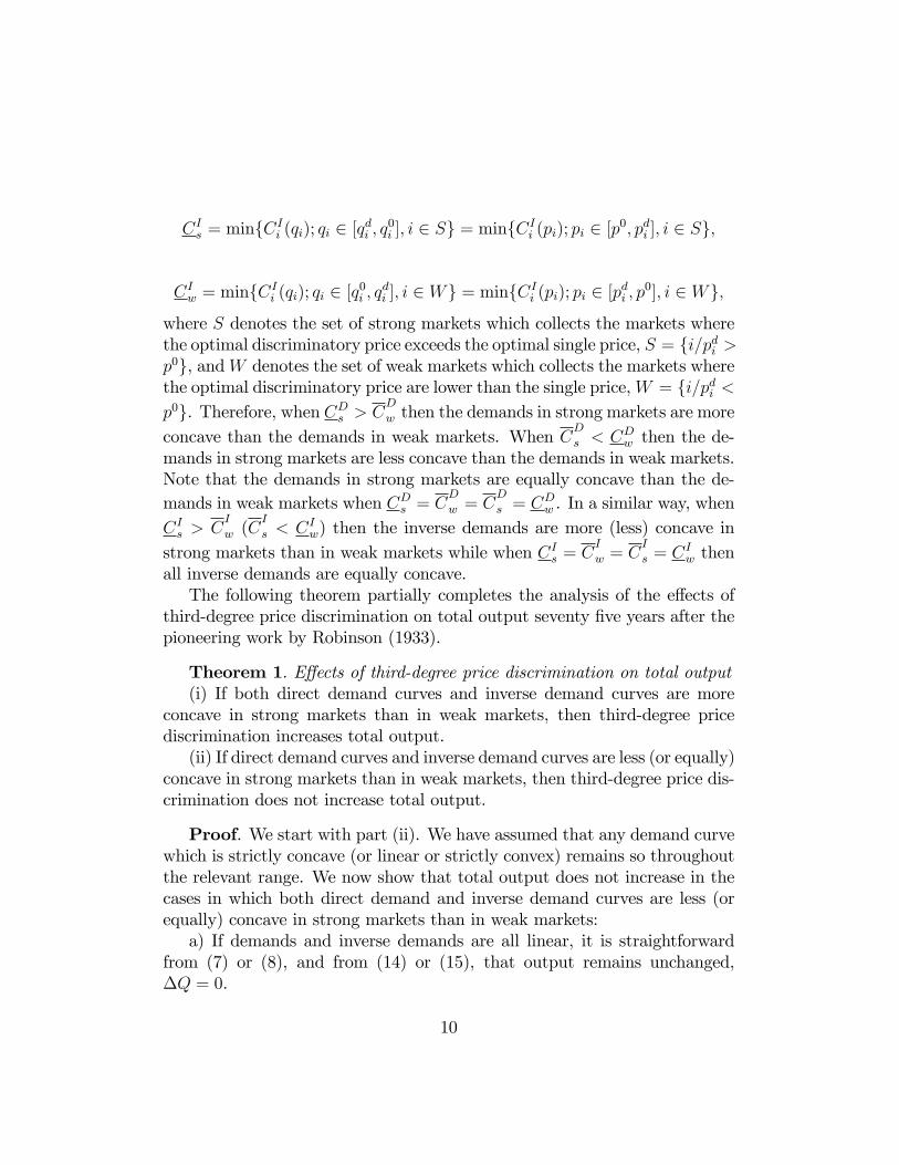
CIs = minfCIi (qi); qi 2 [qdi ; q0i ]; i 2 Sg = minfCIi (pi); pi 2 [p0; pdi ]; i 2 Sg;

CIw = minfCIi (qi); qi 2 [q0i ; qdi ]; i 2 Wg = minfCIi (pi); pi 2 [pdi ; p0]; i 2 Wg;

where S denotes the set of strong markets which collects the markets wherethe optimal discriminatory price exceeds the optimal single price, S = fi=pdi >p0g, andW denotes the set of weak markets which collects the markets wherethe optimal discriminatory price are lower than the single price,W = fi=pdi <p0g. Therefore, when CDs > C

D

w then the demands in strong markets are moreconcave than the demands in weak markets. When C

D

s < CDw then the de-

mands in strong markets are less concave than the demands in weak markets.Note that the demands in strong markets are equally concave than the de-mands in weak markets when CDs = C

D

w = CD

s = CDw . In a similar way, when

CIs > CI

w (CI

s < CIw) then the inverse demands are more (less) concave instrong markets than in weak markets while when CIs = C

I

w = CI

s = CIw then

all inverse demands are equally concave.The following theorem partially completes the analysis of the e¤ects of

third-degree price discrimination on total output seventy �ve years after thepioneering work by Robinson (1933).

Theorem 1. E¤ects of third-degree price discrimination on total output(i) If both direct demand curves and inverse demand curves are more

concave in strong markets than in weak markets, then third-degree pricediscrimination increases total output.(ii) If direct demand curves and inverse demand curves are less (or equally)

concave in strong markets than in weak markets, then third-degree price dis-crimination does not increase total output.

Proof. We start with part (ii). We have assumed that any demand curvewhich is strictly concave (or linear or strictly convex) remains so throughoutthe relevant range. We now show that total output does not increase in thecases in which both direct demand and inverse demand curves are less (orequally) concave in strong markets than in weak markets:a) If demands and inverse demands are all linear, it is straightforward

from (7) or (8), and from (14) or (15), that output remains unchanged,�Q = 0.

10

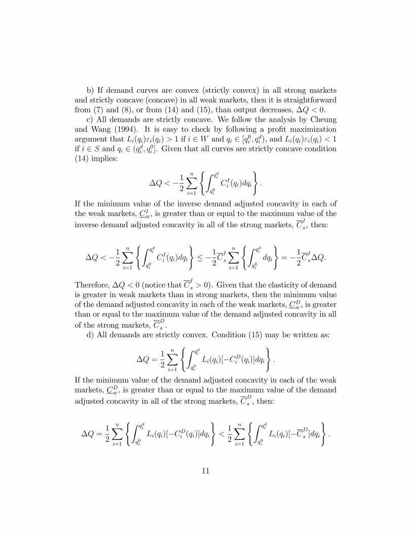
b) If demand curves are convex (strictly convex) in all strong marketsand strictly concave (concave) in all weak markets, then it is straightforwardfrom (7) and (8), or from (14) and (15), than output decreases, �Q < 0.c) All demands are strictly concave. We follow the analysis by Cheung

and Wang (1994). It is easy to check by following a pro�t maximizationargument that Li(qi)"i(qi) > 1 if i 2 W and qi 2 [q0i ; qdi ), and Li(qi)"i(qi) < 1if i 2 S and qi 2 (qdi ; q0i ]. Given that all curves are strictly concave condition(14) implies:

�Q < �12

nXi=1

(Z qdi

q0i

CIi (qi)dqi

):

If the minimum value of the inverse demand adjusted concavity in each ofthe weak markets, CIw, is greater than or equal to the maximum value of theinverse demand adjusted concavity in all of the strong markets, C

I

s, then:

�Q < �12

nXi=1

(Z qdi

q0i

CIi (qi)dqi

)� �1

2CI

s

nXi=1

(Z qdi

q0i

dqi

)= �1

2CI

s�Q:

Therefore, �Q < 0 (notice that CI

s > 0). Given that the elasticity of demandis greater in weak markets than in strong markets, then the minimum valueof the demand adjusted concavity in each of the weak markets, CDw , is greaterthan or equal to the maximum value of the demand adjusted concavity in allof the strong markets, C

D

s .d) All demands are strictly convex. Condition (15) may be written as:

�Q =1

2

nXi=1

(Z qdi

q0i

Li(qi)[�CDi (qi)]dqi

):

If the minimum value of the demand adjusted concavity in each of the weakmarkets, CDw , is greater than or equal to the maximum value of the demandadjusted concavity in all of the strong markets, C

D

s , then:

�Q =1

2

nXi=1

(Z qdi

q0i

Li(qi)[�CDi (qi)]dqi

)<1

2

nXi=1

(Z qdi

q0i

Li(qi)[�CD

s ]dqi

):

11

On the other hand, given that Li(qi) is decreasing in qi,R qdiq0iLi(qi)dqi <R qdi

q0iLi(q

0i )dqi where Li(q

0i ) =

p0�cp0

(see Cheung and Wang, 1994). Therefore,we obtain:

�Q <1

2

nXi=1

(Z qdi

q0i

Li(qi)[�CD

s ]dqi

)=1

2

nXi=1

Li(q0i )[�C

D

s ]

(Z qdi

q0i

dqi

)

=1

2[�CDs ]

p0 � cp0

�Q:

Therefore, �Q < 0 (notice that, from second order conditions, [�CDs ]p0�cp0

<

2). Note also that given that the elasticity of demand is greater in weakmarkets than in strong markets, when 0 > CDw > C

D

s then the minimumvalue of the inverse demand adjusted concavity in each of the weak markets,CIw, is greater than or equal to the maximum value of the inverse demandadjusted concavity in all of the strong markets, C

I

s.

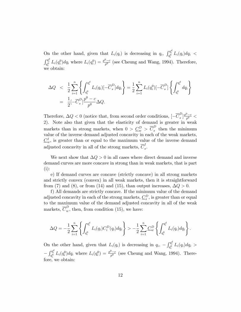
We next show that �Q > 0 in all cases where direct demand and inversedemand curves are more concave in strong than in weak markets, that is part(i):e) If demand curves are concave (strictly concave) in all strong markets

and strictly convex (convex) in all weak markets, then it is straightforwardfrom (7) and (8), or from (14) and (15), than output increases, �Q > 0.f) All demands are strictly concave. If the minimum value of the demand

adjusted concavity in each of the strong markets, CDs , is greater than or equalto the maximum value of the demand adjusted concavity in all of the weakmarkets, C

D

w , then, from condition (15), we have:

�Q = �12

nXi=1

(Z qdi

q0i

Li(qi)CDi (qi)dqi

)> �1

2

nXi=1

CDw

(Z qdi

q0i

Li(qi)dqi

):

On the other hand, given that Li(qi) is decreasing in qi, �R qdiq0iLi(qi)dqi >

�R qdiq0iLi(q

0i )dqi where Li(q

0i ) =

p0�cp0

(see Cheung and Wang, 1994). There-fore, we obtain:

12

�Q > �12

nXi=1

CDwLi(q0i )

(Z qdi

q0i

dqi

)= �1

2CDw

p0 � cp0

�Q:

Therefore, �Q > 0. Note that given that the elasticity of demand is greaterin weak markets than in strong markets, when CDs > C

D

w > 0 then theminimum value of the inverse demand adjusted concavity in each of thestrong markets, CIs, is greater than or equal to the maximum value of theinverse demand adjusted concavity in all of the weak markets, C

I

w.g) All demands are strictly convex. The proof in this case is based on

Cheung and Wang (1994). Given that all curves are strictly convex and thatLi(qi)"i(qi) > 1 if i 2 W and qi 2 [q0i ; qdi ), and Li(qi)"i(qi) < 1 if i 2 S andqi 2 (qdi ; q0i ] then condition (14) implies:

�Q > �12

nXi=1

(Z qdi

q0i

CIi (qi)dqi

):

If the minimum value of the inverse demand adjusted concavity in each ofthe strong markets, CIs, is greater than or equal to the maximum value ofthe inverse demand adjusted concavity in all of the weak markets, C

I

w, thenwe have:

�Q > �12

nXi=1

(Z qdi

q0i

CIi (qi)dqi

)> �1

2CIs

nXi=1

(Z qdi

q0i

dqi

)= �1

2CIs�Q

From second order conditions, 0 > CIs > �2 and therefore �Q > 0. Giventhat the elasticity of demand is greater in weak markets than in strong mar-kets, then the minimum value of the demand adjusted concavity in each ofthe strong markets, CDs , is greater than or equal to the maximum value ofthe demand adjusted concavity in all of the weak markets, C

D

w .�

Note that Theorem 1 a su¢ cient condition for third-degree price dis-crimination to increase total output: if both types of curves, demands andinverse demands, are more concave in the strong markets then price discrimi-nation increases total output. When both types of curves are less (or equally)concave in strong markets than in weak markets then price discriminationreduces (maintains constant) total output. Given Theorem 1 we may con-jecture that a necessary condition for third-degree price discrimination to

13

increase total output is that at least one family of curves, direct or inversedemands, are more concave in strong markets than in weak markets. How-ever, given our concavity comparison criterion we only state that a necessarycondition for price discrimination to increase total output is that both typesof curves cannot be less concave in strong markets than in weak markets. Thenext corollary states necessary conditions and su¢ cient conditions when alldemand curves are strictly concave or strictly convex.

Corollary 1.(i) When all markets have strictly concave demands a su¢ cient (neces-

sary) condition for third-degree price discrimination to increase total outputis that the demands (inverse demands) of the strong markets are more (notless) concave than the demands (inverse demands) of the weak markets.(ii) When all markets have strictly convex demands a necessary (su¢ -

cient) condition for third-degree price discrimination to increase total outputis that the demands (inverse demands) of the strong markets are not less(more) concave than the demands (inverse demands) of the weak markets.

Proof.(i) If the demands of the strong markets are more concave than the de-

mands of the weak markets, CDs > CD

w > 0, then:

CIs �CDs"s>CD

w

"w� CIw;

given that by de�nition strong markets have lower elasticities than weakmarkets. Therefore, both demands and inverse demands are more concave instrong markets than in weak markets and Theorem 1 implies that a su¢ cientcondition for third-degree price discrimination to increase total output issatis�ed.(ii) Assume, on the contrary, that C

D

s < CDw < 0. Then:

CI

s =CD

s

"s<CDw"w

= CIw < 0,

and, therefore, Theorem 1 implies that price discrimination reduces output.�

14

4 Related literature

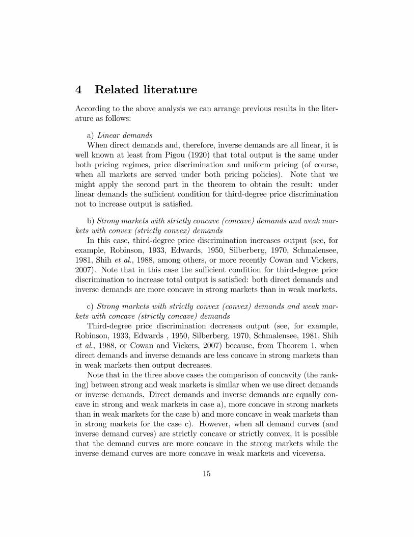
According to the above analysis we can arrange previous results in the liter-ature as follows:

a) Linear demandsWhen direct demands and, therefore, inverse demands are all linear, it is

well known at least from Pigou (1920) that total output is the same underboth pricing regimes, price discrimination and uniform pricing (of course,when all markets are served under both pricing policies). Note that wemight apply the second part in the theorem to obtain the result: underlinear demands the su¢ cient condition for third-degree price discriminationnot to increase output is satis�ed.

b) Strong markets with strictly concave (concave) demands and weak mar-kets with convex (strictly convex) demandsIn this case, third-degree price discrimination increases output (see, for

example, Robinson, 1933, Edwards, 1950, Silberberg, 1970, Schmalensee,1981, Shih et al., 1988, among others, or more recently Cowan and Vickers,2007). Note that in this case the su¢ cient condition for third-degree pricediscrimination to increase total output is satis�ed: both direct demands andinverse demands are more concave in strong markets than in weak markets.

c) Strong markets with strictly convex (convex) demands and weak mar-kets with concave (strictly concave) demandsThird-degree price discrimination decreases output (see, for example,

Robinson, 1933, Edwards , 1950, Silberberg, 1970, Schmalensee, 1981, Shihet al., 1988, or Cowan and Vickers, 2007) because, from Theorem 1, whendirect demands and inverse demands are less concave in strong markets thanin weak markets then output decreases.Note that in the three above cases the comparison of concavity (the rank-

ing) between strong and weak markets is similar when we use direct demandsor inverse demands. Direct demands and inverse demands are equally con-cave in strong and weak markets in case a), more concave in strong marketsthan in weak markets for the case b) and more concave in weak markets thanin strong markets for the case c). However, when all demand curves (andinverse demand curves) are strictly concave or strictly convex, it is possiblethat the demand curves are more concave in the strong markets while theinverse demand curves are more concave in weak markets and viceversa.

15

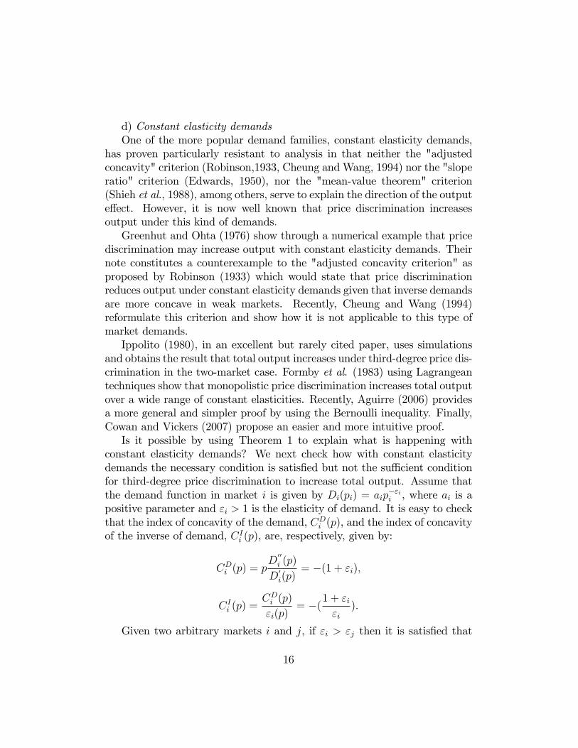
d) Constant elasticity demandsOne of the more popular demand families, constant elasticity demands,

has proven particularly resistant to analysis in that neither the "adjustedconcavity" criterion (Robinson,1933, Cheung andWang, 1994) nor the "sloperatio" criterion (Edwards, 1950), nor the "mean-value theorem" criterion(Shieh et al., 1988), among others, serve to explain the direction of the outpute¤ect. However, it is now well known that price discrimination increasesoutput under this kind of demands.Greenhut and Ohta (1976) show through a numerical example that price

discrimination may increase output with constant elasticity demands. Theirnote constitutes a counterexample to the "adjusted concavity criterion" asproposed by Robinson (1933) which would state that price discriminationreduces output under constant elasticity demands given that inverse demandsare more concave in weak markets. Recently, Cheung and Wang (1994)reformulate this criterion and show how it is not applicable to this type ofmarket demands.Ippolito (1980), in an excellent but rarely cited paper, uses simulations

and obtains the result that total output increases under third-degree price dis-crimination in the two-market case. Formby et al. (1983) using Lagrangeantechniques show that monopolistic price discrimination increases total outputover a wide range of constant elasticities. Recently, Aguirre (2006) providesa more general and simpler proof by using the Bernoulli inequality. Finally,Cowan and Vickers (2007) propose an easier and more intuitive proof.Is it possible by using Theorem 1 to explain what is happening with

constant elasticity demands? We next check how with constant elasticitydemands the necessary condition is satis�ed but not the su¢ cient conditionfor third-degree price discrimination to increase total output. Assume thatthe demand function in market i is given by Di(pi) = aip

�"ii , where ai is a

positive parameter and "i > 1 is the elasticity of demand. It is easy to checkthat the index of concavity of the demand, CDi (p), and the index of concavityof the inverse of demand, CIi (p), are, respectively, given by:

CDi (p) = pD

00i (p)

D0i(p)

= �(1 + "i);

CIi (p) =CDi (p)

"i(p)= �(1 + "i

"i):

Given two arbitrary markets i and j, if "i > "j then it is satis�ed that

16

CDi (p) < CDj (p) and CIi (p) > CIj (p). Therefore, when the criterion of con-

cavity uses inverse demands the ranking of markets is just the opposite tothat when the criterion uses direct demands. In other words, the demandof strong markets is more concave than the demand of the weak marketsand the inverse of demand of strong markets is less concave than the inverseof demand of weak markets: note that CDs > C

D

w and CI

s < CIw. Thatis, according to Theorem 1, the necessary condition is satis�ed but not thesu¢ cient condition for third-degree price discrimination to increase output.

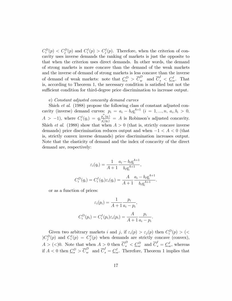
e) Constant adjusted concavity demand curvesShieh et al. (1988) propose the following class of constant adjusted con-

cavity (inverse) demand curves: pi = ai � biqA+1i (i = 1; :::; n; ai; bi > 0;

A > �1), where CIi (qi) = qip00i (qi)

p0i(qi)

= A is Robinson�s adjusted concavity.

Shieh et al. (1988) show that when A > 0 (that is, strictly concave inversedemands) price discrimination reduces output and when �1 < A < 0 (thatis, strictly convex inverse demands) price discrimination increases output.Note that the elasticity of demand and the index of concavity of the directdemand are, respectively:

"i(qi) =1

A+ 1

ai � biqA+1i

biqA+1i

;

CDi (qi) = CIi (qi)"i(qi) =

A

A+ 1

ai � biqA+1i

biqA+1i

:

or as a function of prices:

"i(pi) =1

A+ 1

piai � pi

;

CDi (pi) = CIi (pi)"i(pi) =

A

A+ 1

piai � pi

:

Given two arbitrary markets i and j, if "i(p) > "j(p) then CDi (p) > (<)CDj (p) and C

Ii (p) = CIj (p) when demands are strictly concave (convex),

A > (<)0. Note that when A > 0 then CD

s < CDw and C

I

s = CIw, whereas

if A < 0 then CDs > CD

w and CI

s = CIw. Therefore, Theorem 1 implies that

17

output decreases when demands are strictly concave and output increaseswhen demands are strictly convex.

f) A¢ ne transformations and strictly concave transformations of demandCowan (2007) analyzes the welfare e¤ects of third-degree price discrim-

ination when demand in one market is a shifted version of demand in theother market. In particular, assume that there are only two markets andthe demand in the strong market is an a¢ ne transformation of the demandin the weak market: Ds(p) = � + �Dw(p) with � � 0 and � > 0. It isstraightforward to check that the adjusted concavities are given by:

CDs (p) = CDw (p);

CIs (p) = CIw(p)�

�D00w(p)

�[D0w(p)]

2:

It is easy to �nd examples with strictly convex demands where CD

s � CDw andCI

s < CIw and, therefore, from Theorem 1, output decreases. For example,Cowan (2007) obtains the result that when the underlying demand function,Dw(p), is iso-elastic output decreases.On the other hand, when the demand of the strong market is a strictly

concave transformation of the demand of the weak market,Ds(p) = (Dw(p));

0> 0 and

00< 0, it is easy to �nd examples where output increases. For

example, under iso-elastic demands the demand of the strong market maybe written as a concave transformation of the demand of the weak mar-ket: Ds(p) = (Dw(p)) = k(Dw(p))

"s"w , where k = as(aw)

� "s"w > 0;

0> 0

and 00< 0, and we know that with constant elasticity demands output

increases.Note that in the case of two markets if both the demand and the inverse

demand in the strong market were strictly concave transformations, respec-tively, of the demand and the inverse demand in the weak market then thesu¢ cient condition (from Theorem 1) for third-degree price discriminationto increase output would be satis�ed.

g) Constant inverse demand curvatureCowan and Vickers (2007) propose the following class of constant adjusted

concavity (inverse) demand curves: : pi = ai � bi1+Ai

q1+Aii (ai; bi > 0; Ai 6=

18

�1). Note that the elasticity of demand and the index of concavity of thedirect demand are, respectively:

"i(pi) =1

Ai + 1

piai � pi

;

CIi (pi) = Ai;

CDi (pi) = CIi (pi)"i(pi) =

AiAi + 1

piai � pi

:

Note that this family of demands perfectly illustrates Theorem 1.When demands are strictly concave, given two arbitrary markets i and j, if

"i(p) > "j(p) and Aj > Ai > 0 then CDi (p) < CDj (p) and C

Ii (p) < C

Ij (p). It is

easy to �nd examples where CDs > CD

w and CIs > CI

w (for example, with twomarkets, s and w, as = aw and As > Aw > 0), and therefore where Theorem1 would imply that output increases given that the su¢ cient condition issatis�ed. When "i(p) > "j(p) and Ai > Aj > 0, we have CDi (p) > C

Dj (p) and

CIi (p) > CIj (p). This case is studied by Cowan and Vickers (2007). In their

analysis when CD

s < CDw and CI

s < CIw total output decreases. Note thataccording to Theorem 1 the necessary condition for price discrimination toincrease output is not satis�ed.When demands are strictly convex, given two arbitrary markets i and

j, if "i(p) > "j(p) and 0 > Aj > Ai then CDi (p) < CDj (p) and CIi (p) <

CIj (p). Cowan and Vickers (2007) show that when CDs > C

D

w and CIs > CI

w,output increases. According to Theorem 1 the su¢ cient condition for pricediscrimination to increase output is satis�ed. When "i(p) > "j(p) and 0 >Ai > Aj, we have that CDi (p) > C

Dj (p) and C

Ii (p) > C

Ij (p). It is possible to

�nd examples where CD

s < CDw and C

I

s < CIw, and Theorem 1 implies that

total output decreases.

5 Concluding remarks

The analysis of the e¤ects of third-degree price discrimination on total out-put (and, therefore, on social welfare) has been the focus of much theoreticalresearch at least from the pioneering work by Robinson (1933). In this pa-per, we show that in order for third-degree price discrimination to increase

19

total output the demands of the strong markets should be, as conjecturedby Robinson (1933), in some sense more concave than the demands of theweak markets. By making the distinction between adjusted concavity of theinverse demand and adjusted concavity of the direct demand we are able tostate necessary conditions and su¢ cient conditions for third-degree price dis-crimination to increase total output. The results obtained are rather generaland they seem robust to other cost structure (increasing marginal cost) orto more general comparisons of concavity.Independently, Cowan (2008) has recently obtained su¢ cient conditions

for third-degree price discrimination to increase or to reduce social welfare,being also crucial the relative concavity of the demand and the inverse de-mand of the strong markets in comparison with the weak markets. His resultson welfare nicely complement our results concerning the output e¤ect. Forexample, in his Proposition 2 welfare increases if the inverse demand func-tion in the weak market is more convex at the discriminatory price than theinverse demand in the strong market and the discriminatory prices are close.But then both the direct demand and the inverse demand would be more con-vex in the weak market than in the strong market (the su¢ cient condition,in theorem 1, for third-degree price discrimination to increase total output).Therefore, given that the output increases, the social welfare will increaseif the price di¤erence is small enough that the output e¤ect dominates themisallocation e¤ect.

6 References

Aguirre, I. (2006). �Monopolistic price discrimination and output e¤ectunder conditions of constant elasticity demand�. Economics Bulletin, vol. 4,No 23 pp. 1-6.Aguirre, I. (2008). �Output and misallocation e¤ects in monopolistic

third-degree price discrimination�. Economics Bulletin, vol. 4, No 11 pp.1-6.Battalio, R. C., and Ekelund, R. B. (1972). �Output change under third

degree discrimination�. Southern Economic Journal, vol. 39, pp. 285-290.Bertoletti, P. (2004). �A note on third-degree price discrimination and

output�. Journal of Industrial Economics, vol. 52, No 3, 457; availableat the �Journal of Industrial Economics (JIE) Notes and Comments page�,http:www.essex.ac.uk/jindec/notes.htm.

20

Cheung, F. K., andWang, X. (1994). �Adjusted concavity and the outpute¤ect under monopolistic price discrimination�. Southern Economic Journal,vol. 60, pp. 1048-1054.Cowan, S. (2007). �The welfare e¤ects of third degree price discrimination

with non-linear demand functions�. Rand Journal of Economics, vol. 38, pp.419-428.Cowan, S., and J. Vickers (2007). �Output and welfare e¤ects in the

classic monopoly price discrimination problem�. Discussion paper no 355,Department of Economics, University of Oxford.Cowan, S. (2008). �When does third-degree price discrimination reduce

social welfare, and when does it raise it?�. Discussion paper no 410, Depart-ment of Economics, University of Oxford.Edwards, E. O. (1950). �The analysis of output under discrimination�.

Econometrica, vol. 18, pp. 163-172.Formby, J. P., Layson, S. K. and Smith, W. J. (1983). �Price discrimi-

nation, adjusted concavity, and output changes under conditions of constantelasticity�. Economic Journal, Vol. 93, 892-899.Ippolito, R. A. (1980). �Welfare e¤ects of price discrimination when

demand curves are constant elasticity�. Atlantic Economic Journal, vol. 8,pp. 89-93.Layson, S. K. (1994). �Market opening under third-degree price discrim-

ination�. Journal of Industrial Economics, vol. 42, pp. 335-340.Leontief, W. W. (1940). �The theory of limited and unlimited discrimi-

nation�. Quarterly Journal of Economics, vol. 54, pp. 490-501.Löfgren, K. G. (1977). �A note of output under discrimination�. Rivista

Internacionale di Scienze Economiche, vol. 24, pp. 776-782.Pigou, A.C. (1920). The Economics of Welfare. London: Macmillan.Robinson, J. (1933) (1969, 2ed.). The Economics of Imperfect Competi-

tion. London: Macmillan.Schmalensee, R. (1981). �Output and welfare implications of monopolis-

tic third-degree price discrimination�. American Economic Review, vol. 71,pp. 242-247.Schwartz, M. (1990). �Third-degree price discrimination and output:

generalizing a welfare result�. American Economic Review, vol. 80, pp.1259-1262.Shih, J., Mai, C. and Liu, J. (1988). �A general analysis of the output

e¤ect under third-degree price discrimination�. Economic Journal, vol. 98,pp. 149-158.

21

Silberberg, E. (1970). �Output under discrimination: a revisit�. SouthernEconomic Journal, vol. 37, pp. 84-87.Smith, W. J. and Formby, J. P. (1981). �Output changes under third

degree price discrimination: a re-examination�. Southern Economic Journal,vol. 48, pp. 164-171.Varian, H.R. (1985). �Price discrimination and social welfare�. American

Economic Review, vol. 75, pp. 870-875.

22