Embed Size (px)
Citation preview

J.M. Wrobel - 19 June 2002 SENSITIVITY
1
SENSITIVITY
Outline
What is Sensitivity & Why Should You Care?
What Are Measures of Antenna Performance?
What is the Sensitivity of an Interferometer?
What is the Sensitivity of a Synthesis Image?
Summary

J.M. Wrobel - 19 June 2002 SENSITIVITY
2
What is Sensitivity & Why Should You Care?• Measure of weakest detectable radio emission• Important throughout research program
– Technically sound observing proposal
– Sensible error analysis in publication
• Expressed in units involving Janskys– Unit for interferometer is Jansky (Jy)
– Unit for synthesis image is Jy beam-1
• 1 Jy = 10-26 W m-2 Hz-1 = 10-23 erg s-1 cm-2 Hz-1
• Common to use milliJy or microJy
J.M. Wrobel - 19 June 2002 SENSITIVITY
3
Measures of Antenna Performance
Source and System Temperatures • What is received power P?• Write P as equivalent temperature of matched
termination at receiver input – Rayleigh-Jeans limit to Planck law
– Boltzmann constant kB
– Observing bandwidth
• Amplify P by g2 where g is voltage gain• Separate powers from source, system noise
– Source antenna temperature Ta => source power
– System temperature Tsys => noise power
TkP B
aBa TkgP 2
sysBN TkgP 2
J.M. Wrobel - 19 June 2002 SENSITIVITY
4
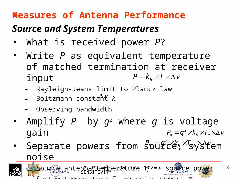
Measures of Antenna Performance
Gain• Source power
– Let for source flux density S, constant K
– Then (1)
• But source power also (2)– Antenna area A, efficiency
– Receiver accepts 1/2 radiation from unpolarized source
• Equate (1), (2) and solve for K
– K is antenna’s gain or “sensitivity”, unit degree Jy-1
• K measures antenna performance but no Tsys
aBa TkgP 2
SKTa SKkgP Ba
2
SAgP aa2
21
a
STkAK aBa /)2/()(

J.M. Wrobel - 19 June 2002 SENSITIVITY
5
Measures of Antenna Performance
System Equivalent Flux Density• Antenna temperature
– Source power
• Express system temperature analogously– Let
– SEFD is system equivalent flux density, unit Jy
– System noise power
• SEFD measures overall antenna performance
– Depends on Tsys and
– Examples in Table 9-1
KTSEFD sys /
SKTa SKkgP Ba
2
SEFDKkgP BN2
)2/()( Ba kAK
SEFDKTsys

J.M. Wrobel - 19 June 2002 SENSITIVITY
6
Interferometer Sensitivity
Real Correlator - 1• Simple correlator with single real output that is
product of voltages from antennas j,i– SEFDi = Tsysi / Ki and SEFDj = Tsysj / Kj
– Each antenna collects bandwidth
• Interferometer built from these antennas has – Accumulation time , system efficiency
– Source, system noise powers imply sensitivity
• Weak source limit – S << SEFDi
– S << SEFDj
acc sijS
acc
ji
sij
SEFDSEFDS
2
1

J.M. Wrobel - 19 June 2002 SENSITIVITY
7
Interferometer Sensitivity
Real Correlator - 2
• For SEFDi = SEFDj = SEFD drop subscripts
– Units Jy
• Interferometer system efficiency – Accounts for electronics, digital losses
– Eg: VLA continuum• Digitize in 3 levels, collect data 96.2% of time
• Effective
s
79.0962.081.0 s
accs
SEFDS
2
1

J.M. Wrobel - 19 June 2002 SENSITIVITY
8
Interferometer Sensitivity
Complex Correlator• Delivers two channels
– Real SR , sensitivity
– Imaginary SI , sensitivity
• Eg: VLBA continuum– Figure 9-1 at 8.4 GHz
– Observed scatter SR(t), SI(t)
– Predicted = 69 milliJy
– Resembles observed scatter
SS
S
accs
SEFDS
2
1

J.M. Wrobel - 19 June 2002 SENSITIVITY
9
Interferometer Sensitivity
Measured Amplitude• Measured visibility amplitude
– Standard deviation (sd) of SR or SI is
• True visibility amplitude S• Probability
– Figure 9-2
– Behavior with true S / • High: Gaussian, sd
• Zero: Rayleigh, sd
• Low: Rice. Sm gives biased estimate of S. Use unbias method.
S
S
22IRm SSS
)/Pr( SSm
S
)2/(2 S

J.M. Wrobel - 19 June 2002 SENSITIVITY
10
Interferometer Sensitivity
Measured Phase• Measured visibility phase
• True visibility phase• Probability
– Figure 9-2
– Behavior with true S /• High: Gaussian
• Zero: Uniform
• Seek weak detection in phase, not amplitude
)Pr( m
S
)/arctan( RIm SS

J.M. Wrobel - 19 June 2002 SENSITIVITY
11
Image Sensitivity
Single Polarization• Simplest weighting case where visibility samples
– Have same interferometer sensitivities
– Have same signal-to-noise ratios w
– Combined with natural weight (W=1), no taper (T=1)
• Image sensitivity is sd of mean of L samples, each with sd , ie,
– No. of interferometers
– No. of accumulation times
– So
int)1(
1
tNN
SEFDI
sm
S
acct /int
)/()1(2
1int acctNNL )1(
2
1 NN
accs
SEFDS
2
1
LSIm /

J.M. Wrobel - 19 June 2002 SENSITIVITY
12
Image Sensitivity
Dual Polarizations - 1• Single-polarization image sensitivity• Dual-polarization data => image Stokes I,Q,U,V
– Gaussian noise in each image
– Mean zero,
• Polarized flux density– Rayleigh noise, sd
– Cf. visibility amplitude, Figure 9-2
• Polarization position angle– Uniform noise between
– Cf. visibility phase, Figure 9-2,
mI
2/mIVUQI 22 UQP
)2/(2)2/(2 UQ
)/arctan(2
1QU
2/

J.M. Wrobel - 19 June 2002 SENSITIVITY
13
Image Sensitivity
Dual Polarizations – 2• Eg: VLBA continuum
– Figure 9-3 at 8.4 GHz
– Observed• T: Stokes I, simplest weighting
• B: Gaussian noise = 90 microJy beam-1
– Predicted
• Previous eg
• Plus here L = 77,200
• So = 88 microJy beam-1
I
I
LSII m 2/2/
S)/()1(
2
1int acctNNL

J.M. Wrobel - 19 June 2002 SENSITIVITY
14
Image Sensitivity
Dual Polarizations – 3• Eg: VLBA continuum
– Figure 9-3 at 8.4 GHz
– Observed• T: Ipeak = 2 milliJy beam-1
• B: Gaussian noise = 90 microJy beam-1
– Position error from sensitivity?
• Gaussian beam = 1.5 milliarcsec
• Then = 34 microarcsec
• Other position errors dominate
I
peakHPBW I
I
2
1
HBPW

J.M. Wrobel - 19 June 2002 SENSITIVITY
15
Image Sensitivity
Dual Polarizations – 4• Eg: VLA continuum
– Figure 9-4 at 1.4 GHz
– Observed• Q, U images, simplest weighting
• Gaussian = 17 microJy beam-1
– Predicted
• = 16 microJy beam-1
accs
SEFDS
2
1
)/()1(2
1int acctNNL
LSIUQ m 2/2/
UQ
UQ
J.M. Wrobel - 19 June 2002 SENSITIVITY
16
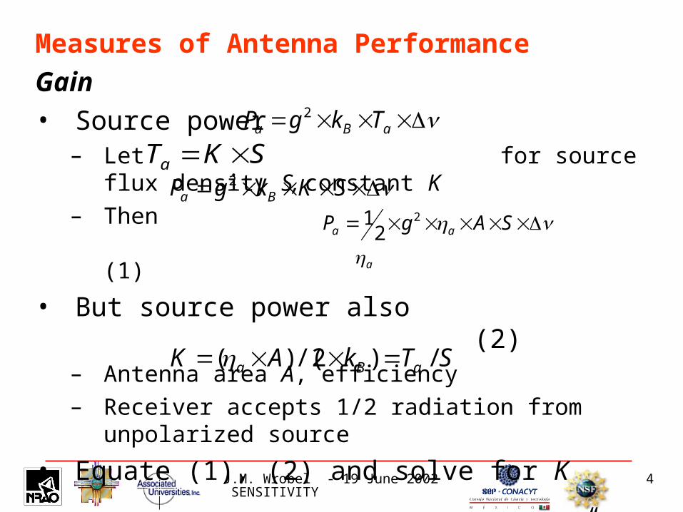
Image Sensitivity
Dual Polarizations – 5• Eg: VLA continuum
– Figure 9-4 at 1.4 GHz
– Observed• Q, U images, simplest weighting
• = 17 microJy beam-1
• Form image of
• Rayleigh noise in P
• Sd 11 microJy beam-1
– Predicted• Sd
• Sd 11 microJy beam-1
22 UQP UQ
)2/(2)2/(2 UQ

J.M. Wrobel - 19 June 2002 SENSITIVITY
17
Image Sensitivity
Dual Polarizations – 6• Eg: VLA continuum
– Figure 9-4 at 1.4 GHz
– Observed• I, Q, U images, simplest weighting
• Gaussian noise
– I, Q, U will have same sd if each is limited by sensitivity• Recall
• Other factors can increase
• Suspect dynamic range as Ipeak = 10,000
• Lesson: Use sensitivity as tool to diagnose problems
II
2/mIVUQI
IUQ

J.M. Wrobel - 19 June 2002 SENSITIVITY
18
Sensitivity
Summary – 1• One antenna
– System temperature Tsys
– Gain K
• Overall antenna performance is measured by system equivalent flux density SEFD
– Units Jy
KTSEFD sys /

J.M. Wrobel - 19 June 2002 SENSITIVITY
19
Sensitivity
Summary - 2• Connect two antennas to form interferometer
– Antennas have same SEFD, observing bandwidth
– Interferometer system efficiency
– Interferometer accumulation time
• Sensitivity of interferometer
– Units Jy
acc
accs
SEFDS
2
1
s

J.M. Wrobel - 19 June 2002 SENSITIVITY
20
Sensitivity
Summary - 3• Connect N antennas to form array
– Antennas have same SEFD, observing bandwidth
– Array has system efficiency
– Array integrates for time tint
– Form synthesis image of single polarization
• Sensitivity of synthesis image
– Units Jy beam-1
int)1(
1
tNN
SEFDI
sm
s