Jitter-minimized reliability-maximized management of networks

Jitter-minimized reliability-maximized management of networks

Waseem Sheikh1,* and Arif Ghafoor2

1Landis+Gyr Inc., 2800 DuncanRoad, Lafayette, IN, USA 47904-50122Department of Electrical and Computer Engineering, Purdue University, West Lafayette, IN, USA

SUMMARY

We propose a joint optimization network management framework for quality-of-service (QoS) routing withresource allocation. Our joint optimization framework provides a convenient way of maximizing thereliability or minimizing the jitter delay of paths. Data traffic is sensitive to droppage at buffers, while it cantolerate jitter delay. On the other hand, multimedia traffic can tolerate loss but it is very sensitive to jitterdelay. Depending on the type of data, our scheme provides a convenient way of selecting the parameterswhich result in either reliability maximization or jitter minimization. We solve the optimization problem fora GPS network and provide the optimal solutions. We find the values of control parameters which controlthe type of optimization performed. We use our analytical results in a multi-objective QoS routing algo-rithm. Finally, we provide insights into our optimization framework using simulations. Copyright © 2011John Wiley & Sons, Ltd.

Received 10 December 2008; Revised 30 January 2010; Accepted 8 February 2010

1. INTRODUCTION

In the last few years, the Internet has become an integral part of our day-to-day life. A growing numberof applications in diverse areas such as personal communications, entertainment, education, telemedi-cine and defense rely on the Internet to transmit multimedia information. As a result, the demand forhigh-quality multimedia information transmitted over the Internet has increased tremendously. Theunderlying networking infrastructure has improved in recent years to provide more resources to usersin order to provide better and reliable data transmission. Despite the continuous improvements innetworking infrastructure, the increasing demand for resource-intensive and QoS-sensitive multimediaservices has increased the need for intelligent and cost-effective network management services.

In order to satisfy the quality-of-service (QoS) requirements for broadband multimedia applications,high-performance communication protocols and networking infrastructure are needed [1]. Suchrequirements pose a broad range of networking challenges for efficient network management, includ-ing resource allocation and intelligent routing. Two major factors affect the QoS requirements:synchronization and reliability. Temporal synchronization at the client [2] is one of the major issues inthe timely transport of multimedia information over a network. Jitter delay experienced over a datanetwork is a major challenge to synchronizing the multimedia stream.

We make the following assumption in our analysis. The reliability value of a link is affected mainlyby data droppage occurring at the output service discipline as a result of buffer overflow. Thisassumption is justified by the fact that packet loss due to corruption during signal propagation alongoptical fibers or coaxial cables tends to be negligible when compared to packet droppage in nodes. Inbroadband networks, losses due to signal corruption are small and negligible. In these networks, the

*Correspondence to: Waseem Sheikh, Senior Software Applications Engineer, Landis+Gyr Inc., 2800 DuncanRoad,Lafayette, IN 47904-5012.

E-mail: [email protected]

INTERNATIONAL JOURNAL OF NETWORK MANAGEMENTInt. J. Network Mgmt 2011; 21: 185–222Published online 27 January 2011 in Wiley Online Library (wileyonlinelibrary.com) DOI: 10.1002/nem.757

Copyright © 2011 John Wiley & Sons, Ltd.

main factor affecting reliability is data droppage at the buffers, due to lack of bandwidth and/or buffer.Lack of bandwidth forces dropping of data irrespective of the traffic characteristics and cannot beavoided. Droppage due to lack of buffer occurs due to burstiness of traffic and either the inability ofthe buffer to absorb such bursts or the lack of the temporarily needed excess bandwidth. The schemeproposed in this paper is for broadband networks where reliability is mostly affected by data droppageat the buffers. Establishing a path with sufficient resources to adequately absorb burstiness is centralto the problem of synchronized multimedia stream delivery. The proposed scheme in this paperestablishes such a path.

This paper deals with the delivery of pre-orchestrated multimedia documents. For this class ofapplications, it is the continuity of presentation rather than the end-to-end delay that dominates theQoS. As a result, the dominating QoS requirements are reliability, bandwidth and jitter. End-to-enddelay has the effect of increasing the start-up time. As long as it is not significantly large (of the orderof several minutes) it does not represent a major degradation in the QoS.

In this paper we consider the problem of jointly optimizing the reliability and jitter delay of pathsunder QoS constraints for a generalized processor sharing (GPS) network [3,4] while reservingbandwidth and buffer at the same time. QoS routing with resource allocation was proposed inBashandy et al. [5], in which the authors only considered maximizing the reliability. However, acertain class of data such as multimedia traffic requires the jitter delay to be minimized. The Internettraffic today consists of a mix of jitter-sensitive traffic such as video and loss-sensitive traffic suchas images and texts. Hence there is a need for a QoS routing scheme which intelligently adapts tothe type of traffic being routed. In this paper we propose a joint optimization framework whichprovides a convenient way of maximizing the reliability or minimizing the jitter delay of the pathsin a network. Multimedia data are sensitive to jitter delay; hence for this kind of data, by selectingappropriate control parameters our problem will find the paths with minimum jitter delay. Datatraffic, on the other hand, can tolerate delay but is sensitive to data drop. For this kind of data,by selecting appropriate control parameters our solution provides the paths with maximumreliability.

This paper is organized as follows. In the next section, we provide an overview of the relatedresearch in the area of QoS routing. In Section 3 we give the formal definition of the multi-objectivepath-resource problem and the multi-objective QoS route problem. Section 4 presents the solution tothe multi-objective path-resource problem for a GPS network. In 5 we present a dynamicprogramming-based algorithm to solve the multi-objective QoS route problem. Simulation results arepresented in Section 6. Finally, we conclude the paper in Section 7.

2. RELATED WORK

In this section we provide an overview of some of the prominent results in the area of QoS routing. Fora detailed survey of the related work in the area of QoS routing please refer to Chen and Nahrstedt [6].The research in this area can be broadly classified into QoS routing with resource consideration andQoS routing without taking resources into account.

In the area of QoS routing with resource consideration [7–9], the network is modeled as a directedgraph with QoS parameters captured as metrics assigned to each edge. Resources are also defined asnumerical values associated with each edge. The metrics associated with each edge are computedbased on the available resources, the traffic description, and, in some cases, the employed servicediscipline. Some of the researchers only consider one resource, which is bandwidth [8,10]. In otherresearch the problem of droppage is not addressed, even though a service discipline is assumed to beemployed [9]. In all the aforementioned work, the allocated resources and the metrics are assumed tobe static and cannot be tweaked during the process of path hunting.

In the area of QoS routing without resource consideration [11–18], the network is modeled as adirected graph G = (V, E). QoS parameters are modeled as functions that map the set of edges E to aset of non-negative integers. These metrics represent the level of QoS provided by each edge. Indetermining these metrics, the interaction between resources is not considered; rather each metric isassumed to be an independent numerical value that can be aggregated using addition. In Wang and

186 W. SHEIKH AND A. GHAFOOR

Copyright © 2011 John Wiley & Sons, Ltd. Int. J. Network Mgmt 2011; 21: 185–222DOI: 10.1002/nem

Crowcroft [18] the authors divided metrics into three categories: additive, multiplicative, and concave(bottleneck). They showed that a combination of one additive or multiplicative metric and one concavemetric is not NP-complete, while a combination of more that one additive and/or multiplicative metricis NP-complete.

Chen and Nahrstedt proposed a heuristic algorithm for the NP-complete multi-path-constrainedrouting problem [19]. The authors show that if all metrics except one take bounded integer values, thenthe multi-path-constrained routing problem is solvable in polynomial time.

Lin and Shroff developed an optimization based approach for QoS routing in high-bandwidthnetworks [20]. The authors take a different view of the network by considering the network (includingthe end-systems and the links) as an integral entity that jointly optimizes some global utility function.Once the solution to the optimization problem is found, the network is driven to an efficient operatingpoint and the routing performance becomes close to optimal. The authors develop an online, distrib-uted algorithm that can efficiently solve the optimization problem. The proposed scheme has theadvantages of reduced computational and communication overhead, analysis of the operating charac-teristics of the network and the ability to tune the desired operating point of the network by choosingappropriate utility functions.

The discussion above highlights the observation that previous research in the field of QoS routingattempts to solve the problem by either modeling the problem as a constrained shortest-path problemwithout considering any resources, or assigning fixed metrics to each link based on the availableresources and the traffic description prior to applying a path search algorithm. These results do notinclude the possibility of tuning the different resources in order to establish a route that simultaneouslysatisfies all the given QoS requirements. Also, the previous efforts do not consider the possibility ofusing the trade-off between QoS parameters to our benefit. For example, suppose the jitter requirementis tight while the droppage requirement is flexible. It may be essential to reduce the jitter resulting fromqueuing delay by reducing the queue size even though we have abundant memory, in order to satisfythe jitter requirement. At the same time, we will not violate the droppage requirement since it is nottight. This implies that assigning the metrics prior to the path search algorithm may preclude findinga path that satisfies the QoS requirements, even though one exists. In addition, the previous results donot incorporate the effect of multiple routers connected in tandem on the QoS parameters of a path;rather addition is used to aggregate the metrics. Also, these results do not include the possibility oftuning the allocated resources during the path search in order to establish a route that simultaneouslysatisfies all the QoS requirements.

Our work is an extension of the framework proposed in Bashandy et al. [5], in which the authorsonly consider reliability as the objective function. However, certain classes of data such as multimediatraffic require the jitter delay to be minimized. Internet traffic today consists of a mix of jitter-sensitivemultimedia traffic and loss-sensitive data traffic. Hence there is a need for a QoS routing scheme whichintelligently adapts to the type of traffic being routed. In this research we propose a joint optimizationframework which provides a convenient way of maximizing the reliability or minimizing the jitterdelay of the paths in a network.

3. PROBLEM DEFINITION

In this section we give the formal definitions of multi-objective path-resource and multi-objective QoSroute problems.

As explained in Section 2, the motivation for formulating the problem as in this section comes fromthe fact that the related research in the area of QoS routing does not provide a single framework thatallows routers and switches to utilize the combined knowledge of hardware/software implementationand the available resources to take intelligent routing decisions.

We consider the following QoS parameters, path jitter delay (Jp), path reliability (Qp), and pathbandwidth (Rp). Let Qreq be the minimum required path reliability, Jreq the maximum required path jit-ter delay, and Rreq the minimum required path bandwidth. The resources are bandwidth and buffer.We denote the buffer at node u of link (u, v) by b(u, v) and the bandwidth for link (u, v) by r(u, v). Let

JITTER-MINIMIZED RELIABILITY-MAXIMIZED MANAGEMENT 187


B(u, v) denote the maximum available buffer at node u, and Cuvmax be the maximum available bandwidth

along link (u, v). Table 1 provides the definitions of symbols used in this paper.Qp is the minimum reliability of the path p. A path p is said to provide a reliability value of Qp if

n

nQp

rec

tran

≥ , where ntran is the total number of bits transmitted at the node at the start of path p and nrec

is the total number of bits received at the end of path p. From the definition of reliability, we haveQp ∈ [0,1].

Instead of minimizing the jitter Jp we minimizeJ

Jp

req

. The minimization ofJ

Jp

req

is the same as the

maximization of −J

Jp

req

or that of 1−⎛⎝⎜

⎞⎠⎟

J

Jp

req

. Note that 1 0 1−⎛⎝⎜

⎞⎠⎟∈[ ]J

Jp

req

, . Hence we define our

objective function as follows: α βQJ

Jp

p+ −⎛⎝⎜

⎞⎠⎟

1req

, where a and b are real numbers selected according

to whether we want to minimize the jitter delay or maximize the reliability.Different researchers [4,11,18,21–25] define the path bandwidth rp(p) as a concave or bottleneck

function of the bandwidths of the links constituting the path. In this paper, we adopt the sameconvention. Hence

r p r u vpu v p

( ) = ( )( )∈min ,

,(1)

In our analysis, we assume that the traffic source is constrained by a leaky bucket [26] policer specifiedby (s, r) where r is the average token rate and s is the bucket size.

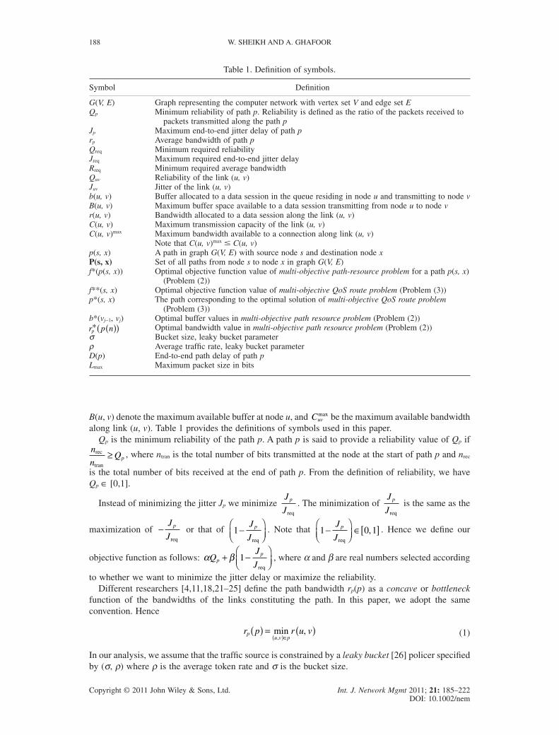
Table 1. Definition of symbols.

Symbol Definition

G(V, E) Graph representing the computer network with vertex set V and edge set EQp Minimum reliability of path p. Reliability is defined as the ratio of the packets received to

packets transmitted along the path pJp Maximum end-to-end jitter delay of path prp Average bandwidth of path pQreq Minimum required reliabilityJreq Maximum required end-to-end jitter delayRreq Minimum required average bandwidthQuv Reliability of the link (u, v)Juv Jitter of the link (u, v)b(u, v) Buffer allocated to a data session in the queue residing in node u and transmitting to node vB(u, v) Maximum buffer space available to a data session transmitting from node u to node vr(u, v) Bandwidth allocated to a data session along the link (u, v)C(u, v) Maximum transmission capacity of the link (u, v)C(u, v)max Maximum bandwidth available to a connection along link (u, v)

Note that C(u, v)max � C(u, v)p(s, x) A path in graph G(V, E) with source node s and destination node xP(s, x) Set of all paths from node s to node x in graph G(V, E)f*(p(s, x)) Optimal objective function value of multi-objective path-resource problem for a path p(s, x)

(Problem (2))f**(s, x) Optimal objective function value of multi-objective QoS route problem (Problem (3))p*(s, x) The path corresponding to the optimal solution of multi-objective QoS route problem

(Problem (3))b*(vj-1, vj) Optimal buffer values in multi-objective path resource problem (Problem (2))r p np* ( )( ) Optimal bandwidth value in multi-objective path resource problem (Problem (2))s Bucket size, leaky bucket parameterr Average traffic rate, leaky bucket parameterD(p) End-to-end path delay of path pLmax Maximum packet size in bits



Let p(v0 = s, v1, v2, . . . , vn-1, vn = x) denote a path with source node s and destination node x. Let{vj|j = 0, 1, . . . , n} be the set of vertices and {(vj-1, vj)|j = 1, 2, . . . , n} the set of edges in this path.Depending on the context in the following discussion, we use symbols p, p(n), and p(s, x) interchange-ably to refer to the path p(v0 = s, v1, v2, . . . , vn-1, vn = x). The multi-objective path-resource problemfor path p is defined as follows:

f p Q pJ p

J

J p J

pp

p

*

Subject to:

req

( ) = ( ) + −( )⎛

⎝⎜⎞⎠⎟

⎧⎨⎩

⎫⎬⎭

( ) ≤

max ,α β 1

rreq

req

req

,

,

, , , ,

, max

Q p Q

b u v B u v u v p

R r u v C

p

uv

( ) ≥≤ ( ) ≤ ( ) ∀( ) ∈

≤ ( ) ≤0

∀∀( )∈∈

u v p, ,

,α β R

(2)

Note that the constraint Rreq � r(u, v) results from adopting the convention that the bandwidth of a pathp is a bottleneck function of the links constituting the path, as specified in equation (1). The decisionvariables in problem (2) are the node buffers b(u, v) and link bandwidth r(u, v) "(u, v) ∈ p. The optimalsolution of problem (2) is denoted by b*(vj-1, vj) and r*(vj-1, vj) for all j = 1, 2, . . . , n.

The multi-objective QoS route problem is defined as follows:

f s x f p s xp s x** *, max ,, ,( ) = ( )( ){ }( )∈ ( )P s x (3)

where P(s, x) is the set of all paths from node s to x. The optimal solution of problem (3) is the pathwhich gives f**(s, x) and is denoted by p*(s, x).

For a GPS network, the QoS parameters as functions of buffers and bandwidth are given asfollows [5].

The minimum reliability Qp(p(n)) for the path p(n) is given by

Q p nb v v

pj n

j j

( )( ) =( ){ }⎧

⎨⎪

⎩⎪

⎫⎬⎪

⎭⎪

≤ ≤−

minmin ,

,11

1σ

(4)

The maximum jitter Jp(p(n)) along the path p(n) is given by

J p n

b v v

r p np

j jj

n

p

( )( ) =( )⎧

⎨⎩

⎫⎬⎭

( )( )

−=∑min , ,1

1

σ(5)

The end-to-end delay for path p(n), denoted by D(p), is given as follows:

D p n J p nL

Cp p

v vj

n

j j

( )( ) = ( )( ) +−( )=

∑ max

,max

11

(6)

where C v vj j−( )1,max is the maximum available physical capacity over the link (vj-1, vj) and Lmax is the

maximum packet size in bits.



For a GPS network, the multi-objective path resource problem can be reformulated as follows:

max minmin ,

,

min , ,

ασ

β11

1

1 1≤ ≤− −( ){ }⎧

⎨⎪

⎩⎪

⎫⎬⎪

⎭⎪+ −

( )j n

j jj jb v v b v v σσ

j

n

pr p n J=∑⎧⎨

⎩

⎫⎬⎭

( )( )

⎛

⎝

⎜⎜⎜⎜

⎞

⎠

⎟⎟⎟⎟

⎧

⎨⎪⎪

⎩⎪⎪

⎫

⎬⎪⎪

⎭⎪⎪

1

req

Subjec

,

tt to: req

min , ,

,

minmin

b v v

r p nJ

b v

j jj

n

p

j n

−=

≤ ≤

( )⎧⎨⎩

⎫⎬⎭

( )( )≤

∑ 11

1

σ

jj jvQ

b u v B u v u v p

R

−( ){ }⎧⎨⎪

⎩⎪

⎫⎬⎪

⎭⎪≥

≤ ( ) ≤ ( ) ∀( ) ∈

1

1

0

,, ,

, , , ,

σ req

req ≤≤ ( ) ≤ ∀( ) ∈∈

r u v C u v puv, ,

,

max

α β R

(7)

Due to the fact that the major contributor of end-to-end delay is the jitter delay, in the later discussionwe only consider the jitter delay.

4. SOLUTION TO THE MULTI-OBJECTIVE PATH RESOURCE PROBLEM

In this section we derive the optimal solutions for the multi-objective path resource problem

defined in (7). For notational simplicity we denote ασ

minmin ,

,1 1 1≤ ≤ −( ){ }⎧⎨⎩

⎫⎬⎭

j n j jb v vby Obj1 and

βσ

111−

( ){ }( )( )

⎛

⎝⎜⎜

⎞

⎠⎟⎟

−=∑min , ,b v v

r p n J

j jj

n

p req

by Obj2. We denote the multi-objective function value by Obj, i.e.,

Obj = Obj1 + Obj2. In all of the following discussion e is a positive real number.

Lemma 1. The optimal value of rp(p(n)) is given by r p n Cp j n v vj j* min ,

max( )( ) = ≤ ≤ ( )−1 1.

Proof. This follows from the fact that the bandwidth of a path is the bottleneck function of thebandwidths of the links constituting the path, and the fact that by increasing the bandwidth the jitterof the path decreases.

Once we have determined the optimal value of bandwidth, we are left with finding the optimal valueof the buffers. �

Theorem 1. If α β σ>( )( )

⎛

⎝⎜

⎞

⎠⎟

n

r p n Jp* req

and J r p n B v vp j jj

n

req * min , ,( )( ) ≥ ( ){ }−=∑σ 11 then the optimal

values of the buffers are given as follows:

b v v B v v j nj jj n

j j* for all−≤ ≤

−( ) = ( ){ } =11

1 1 2, min , min , , , , . . . ,σ

Proof. Let b(vj-1, vj) = b*(vj-1, vj) + e for all j = 1, 2, . . . , n where e is a positive real number.Let the index k be defined as k = arg min1�j�n{B(vj-1, vj)}; then it is not possible to set b(vk-1,vk) = b*(vk-1, vk) + e if B(vk-1, vk) < s. If B(vk-1, vk) � s then Obj1 does not increase; however, Obj2

decreases.Now consider b(vj-1, vj) = b*(vj-1, vj) - e, for all j = 1, 2, . . . , n. Let Objold

i denote the Obji value forb*(vj-1, vj) and let Objnew

i denote the Obji value for b(vj-1, vj) = b*(vj-1, vj) - e for i = 1, 2. We will show



that the multi-objective function value, i.e., Obj, will decrease by changing the buffer values fromb*(vj-1, vj) to b(vj-1, vj).

Obj* *old

11 1 11= ( ){ } = ( ) = (− − −α

σα

σα σ

min,

,, min , ,b v v b v v B v vk k k k k k )){ }

σ

Obj* *new

11 11= ( ) −{ } = ( ) −{ }− −α εσ

ασ

εσ

min,

,,b v v b v vk k k k

Obj Objold new1 1− = αε

σ

Obj*

old

req

2

111= −( ){ }

( )( )

⎧⎨⎪

⎩⎪

⎫⎬⎪

⎭⎪

−=∑β

σmin , ,

*

b v v

r p n J

j jj

n

p

Objnew

req

2

111= −( ){ }

( )( )

⎧⎨⎪

⎩⎪

⎫⎬⎪

⎭⎪

−=∑β

σmin , ,

*

b v v

r p n J

j jj

n

p

Obj Obj*

new old

req

2 2

11− =( ){ }

( )( )−

−=∑β

σβ

min , ,

*

minb v v

r p n J

j jj

n

p

bb v v

r p n J

j jj

n

p

−=( ){ }

( )( )∑ 11

, ,

*

σ

req

Now we have to consider three cases as follows. Case 1 corresponds to when

b v v b v vj jj

n

j jj

n

−= −=( ) < ( ) <∑ ∑11 11

, ,* σ .

Obj Obj*

new old

req

2 2

11 1− =

( )( )( )

−( )−= −∑

β βb v v

r p n J

b v vj jj

n

p

j j,

*

,jj

n

p

p

j jj

n

r p n J

r p n Jb v v n b v

=

−=

∑

∑

( )( )

= −( )( )

( ) − −

1

11

*

*,

req

req

* *β ε jj j

j

n

p

v

n

r p n J

−=

( )⎧⎨⎩

⎫⎬⎭

=( )( )

∑ 11

,

*

εβ

req

The total increase in multi-objective function value is given as follows:

Obj Obj Obj Obj Obj Objnew old new old new old− = − + −

= − +

1 1 2 2

αεσ

εβn

r pp* nn J

n

r p n J

n

r p n Jp p( )( )<

( )( )−

( )( )<

req req req

εβ εσ

β σ* *

0

Hence the net increase in the value of multi-objective function is negative. Therefore

b v v B v vj jj n

j j* −≤ ≤

−( ) = ( ){ }11

1, min , min ,σ

for j = 1, 2, . . . , n is a local optimal solution for case 1.Now we consider case 2, which corresponds to

σ < ( ) < ( )−=

−=

∑ ∑b v v b v vj jj

n

j jj

n

11

11

, ,*

Objold

req

2 1= −( )( )

⎧⎨⎪

⎩⎪

⎫⎬⎪

⎭⎪β σ

r p n Jp*



Objnew

req

2 1= −( )( )

⎧⎨⎪

⎩⎪

⎫⎬⎪

⎭⎪β σ

r p n Jp*

Obj Objnew old2 2 0− =

Obj Objnew old− = −αεσ

Hence in case 2 the multi-objective function value decreases.

Case 3 corresponds to b v v b v vj jj

n

j jj

n

−= −=( ) < < ( )∑ ∑11 11

, ,σ * . In this case the change in multi-

objective function value is computed as follows:

Objold

req

2 1= −( )( )

⎧⎨⎪

⎩⎪

⎫⎬⎪

⎭⎪β σ

r p n Jp*

Objnew

req

2

11

1

1

1

= −( )( )( )

⎧⎨⎪

⎩⎪

⎫⎬⎪

⎭⎪

= −

−=

−

∑β

β

b v v

r p n J

b v

j jj

n

p

j

,

*

,,

*

v n

r p n J

jj

n

p

( ) −( )( )

⎧⎨⎪

⎩⎪

⎫⎬⎪

⎭⎪

=∑ ε1

req

Obj Obj*

new old

req

2 2

11− = −( )

( )( )−

( )(−=∑

β εb v v

r p n J

n

r p n

j jj

n

p p

,

* * ))

⎧⎨⎪

⎩⎪

⎫⎬⎪

⎭⎪+

( )( )

= −( )

( )−=∑

J r p n J

b v v

r p n

p

j jj

n

p

req req

*

βσ

β

*

,

*

11

(( )+

( )( )+

( )( )J

n

r p n J r p n Jp preq req req

β ε β σ* *

Obj Obj*

new old

req

− = −( )

( )( )+

( )( )−=∑

β β εb v v

r p n J

n

r p n

j jj

n

p p

11,

* * JJ r p n J

r p n Jb v v n

p

p

j jj

req req

req

*

+( )( )

−

= −( )( )

( ) − −−

β σ α εσ

β ε σ

*

*,1

==

−=

∑

∑

⎧⎨⎩

⎫⎬⎭−

= −( )( )

( ) −⎧⎨⎩

⎫⎬⎭−

1

11

n

p

j jj

n

r p n Jb v v

α εσ

β σ α εσ*

,req

==( )( )

− ( )⎧⎨⎩

⎫⎬⎭−

<( )( )

−=∑β σ α ε

σ

β

r p n Jb v v

r p n J

p

j jj

n

p

*,

*

req

req

11

σσ εσ

β σ

β

− ( )⎧⎨⎩

⎫⎬⎭−

( )( )

=( )( )

−=∑b v v

n

r p n J

r p n J

j jj

n

p

p

11

,*

*

req

req

σσ ε

β σ ε

− ( ) −⎧⎨⎩

⎫⎬⎭

=( )( )

− ( ) +

−=

−=

∑b v v n

r p n Jb v v

j jj

n

p

j jj

11

1

,

*,

req 11

11

0

n

p

j jj

n

r p n Jb v v

∑

∑

⎛⎝⎜

⎞⎠⎟

⎧⎨⎩

⎫⎬⎭

=( )( )

− ( )⎧⎨⎩

⎫⎬⎭

<

−=

β σ*

,req

*



where the last inequality follows since in this case σ < ( )−=∑ b v vj jj

n* 11

, . This concludes the proof of

Theorem 1. �

Corollary 1.1. The values of a and b can be fixed, for all instances of the path resource allocation

problem in a graph G = (V, E), according to the inequality α β σ> −( )( )( )

N

r p n Jp

1

* req

, where N = �V�.

Proof. Any acyclic path in the directed graph G = (V, E) with vertex set V and edge set E will contain

at most �V� - 1 edges. Let N = �V� - 1; then the constraint α β σ> −( )( )( )

N

r p n Jp

1

* req

impliesα β σ>

( )( )n

r p n Jp* reqfor any n � (N - 1). �

Theorem 2. If α β σ<( )( )

⎛

⎝⎜

⎞

⎠⎟

n

r p n Jp* req

, J r p n B v vp j jj

n

req * min , ,( )( ) ≥ ( ){ }−=∑σ 11and nQreq � 1, then

the optimal values of the buffers are given as follows:

b v v B v v j nj jj n

j j* , for all−≤ ≤

−( ) = ( ){ } =11

1 1 2, min , min , , , . . . ,σ

Proof. Let b(vj-1, vj) = b*(vj-1, vj) + e for all j = 1, 2, . . . , n where e is a positive real number. Let theindex k be defined as k = arg min 1�j�n{B(vj-1, vj)}; then it is not possible to set b(vk-1, vk) = b*(vk-1,vk) + e if B(vk-1, vk) < s. If B(vk-1, vk) � s then the multi-objective function value does not change byincreasing the values of buffers.

Now consider b(vj-1, vj) = b*(vj-1, vj) - e for all j = 1, 2, . . . , n.

Obj*old

11

1

1

1

= ( )⎧⎨⎩

⎫⎬⎭

= ( ){ }{−

−

ασ

α σσ

min,

,

minmin , ,

,

b v v

B v v

j j

k k }}= ( ){ }

= ( )

−

−

α σσ

ασ

min , ,

,

B v v

b v v

k k

j j

1

1*

Obj

*

new1

1

1

1

1

= ( )⎧⎨⎩

⎫⎬⎭

= ( ) −⎧⎨⎩

⎫⎬⎭

−

−

ασ

αε

σ

min,

,

min,

,

b v v

b v v

j j

j j

== ( ) −−αε

σb v vj j* 1,

Obj Obj* *new old

1 11 1− = ( ) − − ( )

= −

− −αε

σα

σ

α εσ

b v v b v vj j j j, ,

Note that the value of Obj2 does not change if we replace b*(vj-1, vj) with any feasible b(vj-1, vj). The

reason for this is since σ σ σ≤ = ≤ ( )= −=∑ ∑n Q Q b v v

j

n

j jj

n

req req1 11, for all positive e that results in a

feasible value for the buffer variables b(vj-1, vj). The first inequality (from the left-hand side) in theabove is true by assumption in the theorem and the last inequality holds because of the minimumreliability constraint. Hence the multi-objective function value decreases by decreasing the value of the



buffers. Therefore, under the assumptions in Theorem 2, the optimal buffer values are given

by b v v B v vj jj n

j j* −≤ ≤

−( ) = ( ){ }11

1, min , min ,σ , for all j = 1, 2, . . . , n. This concludes the proof of

Theorem 2. �


−−

⎛

⎝⎜

⎞

⎠⎟

r p n J

nQ

Qp* req

req

req

1

1, where 0 � Qreq < 1, J r p npreq * ( )( ) ≥

min , ,σ B v vj jj

n

−=( ){ }∑ 11

and nQreq < 1, then the optimal values of the buffers are given by

b v v Q j nj j* for allreq−( ) = =1 1 2, , , , . . . ,σ

Proof. Let b(vj-1, vj) = b*(vj-1, vj) - e for all j = 1, 2, . . . , n where e is a positive real number. This wouldviolate the minimum reliability constraint. Now consider b(vj-1, vj) = b*(vj-1, vj) + e for all j = 1, 2, . . . ,n. We will show that under the assumptions of Theorem 3 the increase in Obj1 will be less than thedecrease in Obj2 for all positive e.

Obj*old

req

req

11 1

1

1

= ( )⎧⎨⎩

⎫⎬⎭

= { }=

−ασ

ασσ

α

min,

,

min ,

min ,

b v v

Q

Q

j j

{{ }= αQreq

Obj

*

new1

1

1

1

1

= ( )⎧⎨⎩

⎫⎬⎭

= ( ) +⎧⎨⎩

⎫⎬⎭

−

−

ασ

αε

σ

min,

,

min,

,

b v v

b v v

j j

j j

== +{ }≤ +{ }α ε

σ

α εσ

min ,Q

Q

req

req

1

Obj Objnew oldreq req1 1− ≤ +{ }−

=

α εσ

α

α εσ

Q Q

In order to find the corresponding decrease in Obj2 we have to consider two cases. In case 1n(sQreq + e) < s. The decrease in Obj2 for case 1 is given as follows:

Objold req

req

req

2 1

1

= − { }( )( )

⎧⎨⎪

⎩⎪

⎫⎬⎪

⎭⎪

= −

βσ σ

βσ

min ,

*

n Q

r p n J

n Q

r

p

pp p n J* ( )( )

⎧⎨⎪

⎩⎪

⎫⎬⎪

⎭⎪req



where the last equality follows from the inequality nQreq < 1 in the hypothesis of Theorem 3.

Objnew req

req

r

2 1

1

= −+{ }

( )( )

⎧⎨⎪

⎩⎪

⎫⎬⎪

⎭⎪

= −

βσ ε σ

βσ

min ,

*

n Q n

r p n J

n Q

p

eeq

req

+

( )( )

⎧⎨⎪

⎩⎪

⎫⎬⎪

⎭⎪

n

r p n Jp

ε*

where the last equality follows since under case 1, i.e., nQreq + ne < s.

Obj Objold new req

req

req2 2 1 1− = −

( )( )

⎧⎨⎪

⎩⎪

⎫⎬⎪

⎭⎪− −β

σβ

σn Q

r p n J

n Q

p*

++

( )( )

⎧⎨⎪

⎩⎪

⎫⎬⎪

⎭⎪

=( )( )

n

r p n J

n

r p n J

p

p

ε

β ε

*

*

req

req

Obj Objnew old

req

req

− ≤ −( )( )

<( )( )

−

α εσ

β ε

β σ εσ

β ε

n

r p n J

n

r p n J

n

r

p

p

*

* pp p n J* ( )( )=

req

0

In case 2, n(Qreq + e) � s. In this case the decrease in Obj2 will not depend on e; hence it is sufficientto show that under the assumptions of Theorem 3 the maximum increase in Obj1 is less than the fixeddecrease in Obj2.

Objold req

req

req

1 1

1

= { }= { }=

ασσ

αα

min ,

min ,

Q

Q

Q

Objnew req

req

1 1

1

=+{ }

= +{ }α

σ εσ

α εσ

min ,

min ,

Q

Q

Obj Objnew oldreq req1 1 1− = +{ }−α ε

σαmin ,Q Q

max Obj Objnew oldreq

req

1 1

1

−{ } = −

= −( )α αα

Q

Q

Objold req

req

req

2 1

1

= − { }( )( )

⎧⎨⎪

⎩⎪

⎫⎬⎪

⎭⎪

= −

βσ σ

βσ

min ,

*

n Q

r p n J

n Q

r

p

pp p n J* ( )( )

⎧⎨⎪

⎩⎪

⎫⎬⎪

⎭⎪req



Objnew req

req

2 1

1

= −+{ }

( )( )

⎧⎨⎪

⎩⎪

⎫⎬⎪

⎭⎪

= −

βσ ε σ

β σ

min ,

*

*

n Q n

r p n J

r

p

p pp n J( )( )

⎧⎨⎪

⎩⎪

⎫⎬⎪

⎭⎪req

where the last equality for Objold2 follows from the hypothesis of Theorem 3, namely, nQreq < 1, and the

last equality for Objnew2 follows from the hypothesis of case 2, i.e., nQreq + ne � s.

Obj Objold new req

req req

2 2− = −( )( )

− +( )( )

=

β βσ

β β σ

β

n Q

r p n J r p n Jp p* *

σσ

r p n JnQ

p* ( )( )−{ }

req

req1

Obj Objnew oldreq

req

req− = −( ) −( )( )

−{ }

<

α β σ1 1

0

Qr p n J

nQp*

where the last inequality follows from the hypothesis in Theorem 3 specifically,

α β σ<( )( )

−−

⎛

⎝⎜

⎞

⎠⎟

r p n J

nQ

Qp* req

req

req

1

1. This concludes the proof of Theorem 3. �

In order for the dynamic programming algorithm to find optimal paths, the values of a and b haveto be fixed and should not vary as the number of nodes in the path change. The following corollary toprevious theorems provides a fixed value for a and b depending upon whether we want to maximizereliability or minimize the jitter delay.

Corollary 3.1. The values of a and b can be fixed, for all instances of the path resource allocation

problem in a graph G = (V, E), according to the inequality β ασ

>( )( ) −

−r p n J Q

n Qp* req req

req*

1

1, where

nQ

* =⎡

⎢⎢

⎤

⎥⎥ −

11

req

.

Proof. Note that we have 1 - Qreq > 1 - nQreq for 11< <n

Qreq

. In other words,1

11

−−

>Q

nQreq

req

for

11< <n

Qreq

. Hence:

β ασ

β ασ

>( )( ) −

−

⎛

⎝⎜

⎞

⎠⎟ ⇒ >

( )( )⎛

⎝⎜

r p n J Q

nQ

r p n J

np p* *req req

req

req1

1

⎞⎞

⎠⎟

for 11< <n

Qreq

.

Let nQ

* =⎡

⎢⎢

⎤

⎥⎥ −

11

req

. We have the following inequality:

1

1

1

1

−−

≥−−

Q

n Q

Q

nQreq

req

req

req*



for all 11< <n

Qreq

. This implies that we can select the values of a and b using the inequality

β ασ

>( )( ) −

−r p n J Q

n Qp* req req

req*

1

1, where n

Q* =

⎡

⎢⎢

⎤

⎥⎥ −

11

req

. �

Theorem 4. If α β σ>( )( )

⎛

⎝⎜

⎞

⎠⎟

n

r p n Jp* req

and J r p n B v vp j jj

n

req * min , ,( )( ) ≤ ( ){ }−=∑σ 11, then the optimal

values of the buffers are given as follows:

b v v B v vJ r p n

nj j

j nj j

req p* −≤ ≤

−( ) = ( ) ( )( )⎧⎨⎪

⎩⎪

⎫⎬1

11, min min min , ,

* ⎪⎪

⎭⎪

⎧⎨⎪

⎩⎪

⎫⎬⎪

⎭⎪=

,

, , . . . , .

σ

for all j n1 2

(8)

Proof. Note that the inequality J r p n B v vp j jj

n

req * min , ,( )( ) ≤ ( ){ }−=∑σ 11means that the maximum

number of bits queued in the buffers on the path p(n) can lead to a violation of the jitter constraint. Letk = arg min1�j�n{B(vj-1, vj)}.

Depending upon the ordering of B(vk-1, vk),J r p n

npreq * ( )( )

and s we have to consider four different

cases. Case 1 corresponds to when B v vJ r p n

nk k

p−( ) < ( )( )

1,*req and B(vk-1, vk) < s. In this case the

optimal buffer value in equation 8 reduces to b*(vj-1, vj) = B(vk-1, vk) + e for all j = 1, 2, . . . , n.Now consider b(vj-1, vj) = b*(vj-1, vj) + e where e is a positive real number. However, settingb(vk-1, vk) = B*(vk-1, vk) + e will result in the violation of the available physical buffer constraint onnode k. Therefore, we only need to consider b(vj-1, vj) = b*(vj-1, vj) - e for all j = 1, 2, . . . , n.

Obj*old

11

1

= ( )

= ( )

−

−

ασ

ασ

b v v

B v v

j j

k k

,

,

Objnew1

1

1

1

= ( )

= ( ) −

= ( ) −

−

−

−

ασ

α εσ

ασ

α εσ

b v v

B v v

B v v

j j

k k

k k

,

,

,

Obj Objnew old1 1− = −α ε

σ

Obj*

old

req

2

111= −( ){ }

( )( )

⎧⎨⎪

⎩⎪

⎫⎬⎪

⎭⎪

=

−=∑β

σmin , ,

*

b v v

r p n J

j jj

n

p

ββ σ1 1− ( ){ }

( )( )

⎧⎨⎪

⎩⎪

⎫⎬⎪

⎭⎪−min , ,

*

nB v v

r p n J

k k

p req

Objnew

req

211= − ( ) −( ){ }

( )( )

⎧⎨⎪

⎩⎪

⎫⎬⎪

⎭⎪−β ε σmin , ,

*

n B v v

r p n J

k k

p



Let case 1(a) correspond to when n(B(vk-1, vk) - e) < nB(vk-1, vk) < s. In this case the net change in themulti-objective function value is given as follows:

Objold

req

211= − ( )

( )( )

⎧⎨⎪

⎩⎪

⎫⎬⎪

⎭⎪−β nB v v

r p n J

k k

p

,

*

Objnew

req

211= − ( ) −(

( )( )

⎧⎨⎪

⎩⎪

⎫⎬⎪

⎭⎪−β εn B v v

r p n J

k k

p

,

*

Obj Objnew old

req

2 2− =( )( )

β εn

r p n Jp*

Obj Objnew old

req

req

− = − +( )( )

=( )( )

−

<

α εσ

β ε

β ε α εσ

β

n

r p n J

n

r p n J

p

p

*

*

nn

r p n J

n

r p n Jp p

ε β σ εσ* *( )( )

−( )( )

<req req

0

Case 1(b) corresponds to when s < n(B(vk-1, vk) - e) < nB(vk-1, vk) < s. In this case the net change in themulti-objective function value is given as follows:

Objold

req

2 1= −( )( )

⎧⎨⎪

⎩⎪

⎫⎬⎪

⎭⎪β σ

r p n Jp*

Objnew

req

2 1= −( )( )

⎧⎨⎪

⎩⎪

⎫⎬⎪

⎭⎪β σ

r p n Jp*


Obj Objnew old− = −

<

α εσ

0

Case 1(c) corresponds to when n(B(vk-1, vk) - e) < s < nB(vk-1, vk) < s. In this case the net change in themulti-objective function value is given as follows:

Objold

req

2 1= −( )( )

⎧⎨⎪

⎩⎪

⎫⎬⎪

⎭⎪β σ

r p n Jp*

Objnew

req

211= − ( ) −( )( )

⎧⎨⎪

⎩⎪

⎫⎬⎪

⎭⎪−β εnB v v n

r p n J

k k

p

,

*



Obj Objnew old

req r

2 21− = − ( )

( )( )+

( )( )−β β β εnB v v

r p n J

n

r p n J

k k

p p

,

* * eeq req

req

− +( )( )

=( )( )

+ − ( ){ }

=

−

β β σ

β σ ε

β

r p n J

r p n Jn nB v v

r

p

p

k k

p

*

*,1

**,

*,

p n Jn B v v

r p n JnB v v

k k

p

k k

( )( )− ( ) −( ){ }

<( )( )

( ) −

−

−

req

req

σ ε

β

1

1 nn B v v

n

r p n J

k k

p

−( ) −( ){ }

=( )( )

1,

*

ε

β ε

req

Obj Objnew old

req

− <( )( )

−

<

β ε α εσ

n

r p n Jp*

0

This concludes the treatment for case 1. Now for case 2, assume that B v vJ r p n

nk k

p−( ) < ( )( )

1,*req and

B(vk-1, vk) > s. In this case the optimal buffer values given by equation (8) reduces to b*(vj-1, vj) = s,for all j = 1, 2, . . . , n. Let b(vj-1, vj) = b*(vj-1, vj) + e, where e is some positive real number. Thenincreasing the buffer values from b*(vj-1, vj) = s to b(vj-1, vj) = s + e does not change the Obj1;however, it results in a decrease in Obj2 value.

Now consider b(vj-1, vj) = b*(vj-1, vj) - e = s - e. The change in multi-objective function value iscomputed as below.

Objold1 = α

Objnew1 = −α σ ε

σ

Obj Objnew old1 1− = − −

= −

α σ εσ

α

α εσ

Objold

req

2 1= −( )( )

⎧⎨⎪

⎩⎪

⎫⎬⎪

⎭⎪β σ

r p n Jp*

Objnew

req

2

111= −( ){ }

( )( )

⎧⎨⎪

⎩⎪

⎫⎬⎪

⎭⎪

−=∑β

σmin , ,

*

b v v

r p n J

j jj

n

p

Let case 2(a) correspond to when σ ≤ ( )−=∑ b v vj jj

n

11, .

Objold

req

2 1= −( )( )

⎧⎨⎪

⎩⎪

⎫⎬⎪

⎭⎪β σ

r p n Jp*



Objnew

req

2 1= −( )( )

⎧⎨⎪

⎩⎪

⎫⎬⎪

⎭⎪β σ

r p n Jp*



<

α εσ

0

Case 2(b) corresponds to when σ > ( )−=∑ b v vj jj

n

11, , i.e., s > n(s - e). The change in multi-

objective function is computed as below:

Objold

req

2 1= −( )( )

⎧⎨⎪

⎩⎪

⎫⎬⎪

⎭⎪β σ

r p n Jp*

Objnew

req

2

111

1

= −( )( )( )

⎧⎨⎪

⎩⎪

⎫⎬⎪

⎭⎪

= − −(

−=∑β

β σ ε

b v v

r p n J

n

j jj

n

p

,

*

))( )( )

⎧⎨⎪

⎩⎪

⎫⎬⎪

⎭⎪r p n Jp* req

Obj Objnew old

req

2 2 1 1− = − −( )( )( )

⎧⎨⎪

⎩⎪

⎫⎬⎪

⎭⎪− −β σ ε β σn

r p n J r p np p* * (( )( )

⎧⎨⎪

⎩⎪

⎫⎬⎪

⎭⎪

=( )( )

− −( )( )( )

=

J

r p n J

n

r p n Jp p

req

req req

β σ β σ ε

β

* *

rr p n Jn

p* ( )( )− −( ){ }

req

σ σ ε

Obj Objnew old

req

req

− =( )( )

− −( ){ }−

<( )( )

β σ σ ε α εσ

β σ

r p n Jn

r p n J

p

p

*

*−− −( ){ }−

( )( )

=( )( )

−( )( )

nn

r p n J

r p n J

n

r p n

p

p p

σ ε β σ εσ

β σ β σ

*

* *

req

req JJ

n

r p n J

n

r p n J

r p n Jn

p p

p

req req req

req

+( )( )

−( )( )

=( )( )

−

β ε β ε

β σ

* *

*1(( )

≤ 0

for n = 1, 2, 3, . . . .

Case 3 corresponds to B v vJ r p n

nk k

p−( ) > ( )( )

1,*req and B(vk-1, vk) > s. Let case 3(a) add the

additional constraint,J r p n

npreq * ( )( )

< σ to the aforementioned two constraints in case 3. In case 3(a),

the optimal buffer value given by equation (8) reduces to b v vJ r p n

nj j

p* req−( ) = ( )( )

1,*

. Let



b v v b v vJ r p n

nj j j j

p− −( ) = ( ) + =

( )( )+1 1, ,

** reqε ε for some j. This, however, violates the maximum physi-

cal buffer constraint for node j. Now set b v v b v vJ r p n

nj j j j

p− −( ) = ( ) − =

( )( )−1 1, ,

** reqε ε for all j = 1,

2, . . . , n and for 0 < ≤( )( )

εJ r p n

npreq *

. The change in multi-objective function value for case 3(a) is

computed below.

Objold req1 =

( )( )α

σJ r p n

np*

Objnew req1 =

( )( )−

⎧⎨⎪

⎩⎪

⎫⎬⎪

⎭⎪α

σεσ

J r p n

np*

Obj Objnew old req req1 1− =

( )( )−

⎧⎨⎪

⎩⎪

⎫⎬⎪

⎭⎪−

( )α

σεσ

αJ r p n

n

J r p np p* *(( )

= −

nσ

α εσ

Obj*

old

req

2

111= −( ){ }

( )( )

⎧⎨⎪

⎩⎪

⎫⎬⎪

⎭⎪

−=∑β

σmin , ,

*

b v v

r p n J

j jj

n

p

Objnew

req

2

111= −( ){ }

( )( )

⎧⎨⎪

⎩⎪

⎫⎬⎪

⎭⎪

−=∑β

σmin , ,

*

b v v

r p n J

j jj

n

p

Let case 3(a)(i) correspond to when b v v b v vj jj

n

j jj

n

−= −=( ) < ( ) <∑ ∑11 11

, ,* σ , or equivalently,

( * ) ( * )r p n J n r p n Jp p( )( ) − < ( )( ) <req reqε σ . In case 3(a)(i) the change in multi-objective function is

computed as follows:

Objold req

req

2 1

0

= −( )( )( )( )

⎧⎨⎪

⎩⎪

⎫⎬⎪

⎭⎪=

βr p n J

r p n J

p

p

*

*

Objnew req

req

2 1= −( )( ) −

( )( )

⎧⎨⎪

⎩⎪

⎫⎬⎪

⎭⎪

=

βε

β ε

r p n J n

r p n J

n

r p

p

p

p

*

*

* nn J( )( ) req

Obj Objnew old

req

2 2− =( )( )

β εn

r p n Jp*



Obj Objnew old

req

req

− =( )( )

−

<( )( )

−

β ε α εσ

β ε β εσ

σ

n

r p n J

n

r p n J

n

r

p

p

*

* pp p n J* ( )( )=

req

0

In case 3(a)(ii) we have σ < ( ) < ( )−= −=∑ ∑b v v b v vj jj

n

j jj

n

11 11, ,* . The change in multi-objective func-

tion value for this case is computed below:

Objold

req

2 1= −( )( )

⎧⎨⎪

⎩⎪

⎫⎬⎪

⎭⎪β σ

r p n Jp*

Objnew

req

2 1= −( )( )

⎧⎨⎪

⎩⎪

⎫⎬⎪

⎭⎪β σ

r p n Jp*



<

α εσ

0

In case 3(a)(iii) we have b v v b v vj jj

n

j jj

n

−= −=( ) < < ( )∑ ∑11 11

, ,σ * :

Objold

req

2 1= −( )( )

⎧⎨⎪

⎩⎪

⎫⎬⎪

⎭⎪β σ

r p n Jp*

Objnew req

req

2 1= −( )( ) −

( )( )

⎧⎨⎪

⎩⎪

⎫⎬⎪

⎭⎪

=

βε

β ε

r p n J n

r p n J

n

r p

p

p

p

*

*

* nn J( )( ) req

Obj Objnew old

req req

2 2− =( )( )

− +( )( )

β ε β β σn

r p n J r p n Jp p* *

Obj Objnew old

req req

− =( )( )

− +( )( )

−

<

β ε β β σ α εσ

β ε

n

r p n J r p n J

n

r

p p

p

* *

** * *

*

p n J r p n J

n

r p n J

r p n

p p

p

( )( )− +

( )( )−

( )( )

=(

req req req

β β σ β εσ

σ

β σ

))( )−

⎧⎨⎪

⎩⎪

⎫⎬⎪

⎭⎪<

Jreq

1

0

where the last inequality follows since σ < ( )( )r p n Jp* req .



Now we consider case 3(b), corresponding to the additional constraintJ r p n

npreq * ( )( )

> σ , in addition

to the constraints corresponding to case 3. In this case the optimal buffer value given by equation (8)reduces to b*(vj-1, vj) = s for all j = 1, 2, . . . , n.

First, consider b(vj-1, vj) = b*(vj-1, vj) + e = s + e, for all j = 1, 2, . . . , n. However, as a result ofthis increase in buffer values Obj1 value does not change and Obj2 value decreases. Now considerb(vj-1, vj) = b*(vj-1, vj) - e = s - e for all j = 1, 2, . . . , n. The change in multi-objective functionvalue is computed below:

Objold1 = α

Objnew1 = −

= −

α σ εσ

α α εσ


σ

Obj*

old

req

2

111= −( ){ }

( )( )

⎧⎨⎪

⎩⎪

⎫⎬⎪

⎭⎪

=

−=∑β

σmin , ,

*

b v v

r p n J

j jj

n

p

ββ σ σ

β σ

1

1

− { }( )( )

⎧⎨⎪

⎩⎪

⎫⎬⎪

⎭⎪

= −( )( )

⎧⎨⎪

⎩

min ,

*

*

n

r p n J

r p n J

p

p

req

req⎪⎪

⎫⎬⎪

⎭⎪

Objnew

req

2

111= −( ){ }

( )( )

⎧⎨⎪

⎩⎪

⎫⎬⎪

⎭⎪

=

−=∑β

σ

β

min , ,

*

b v v

r p n J

j jj

n

p

11− −( ){ }( )( )

⎧⎨⎪

⎩⎪

⎫⎬⎪

⎭⎪

min ,

*

n

r p n Jp

σ ε σ

req

Let case 3(b)(i) correspond to when s < n(s - e).

Objnew

req

2 1= −( )( )

⎧⎨⎪

⎩⎪

⎫⎬⎪

⎭⎪β σ

r p n Jp*



<

α εσ

0

Case 3(b)(ii) corresponds to n(s - e) < s :

Objnew

req

2 1= − −( )( )( )

⎧⎨⎪

⎩⎪

⎫⎬⎪

⎭⎪β σ εn

r p n Jp*



Obj Objnew old

req

2 2 1 1− = − −( )( )( )

⎧⎨⎪

⎩⎪

⎫⎬⎪

⎭⎪− −β σ ε β σn

r p n J r p np p* * (( )( )

⎧⎨⎪

⎩⎪

⎫⎬⎪

⎭⎪

=( )( )

− −( )( )( )

⎧⎨⎪

J

r p n J

n

r p n Jp p

req

req req

β σ σ ε* *⎩⎩⎪

⎫⎬⎪

⎭⎪

=( )( )

− −( ){ }β σ σ εr p n J

np* req

Obj Objnew old

req

req

− =( )( )

− −( ){ }−

<( )( )

β σ σ ε α εσ

β σ

r p n Jn

r p n J

p

p

*

*−− −( ){ }−

( )( )

=( )( )

−( )

≤

nn

r p n J

r p n Jn

p

p

σ ε β εσ

σ

β σ

*

*

req

req

1

0

for n = 1, 2, 3, . . . .

Case 4 corresponds to the inequalitiesJ r p n

nB v vp

k kreq *

,( )( )

< ( )−1 and B(vk-1, vk) < s. In this case the

optimal buffer values given by equation (8) reduce to b v vr p n J

nj j

p* req−( ) = ( )( )

1,*

for all j = 1, 2,

3, . . . , n. First consider b(vj-1, vj) = b*(vj-1, vj) + e. This results in violation of the jitter constraint. Now

consider b v v b v vr p n J

nj j j j

p− −( ) = ( ) − =

( )( )−1 1, ,

** reqε ε for all j = 1, 2, 3, . . . , n.

Objold req1 =

( )( )α

σr p n J

np*

Objnew req1 =

( )( )−α

σα ε

σr p n J

np*


σ

Obj*

old

req

2

111= −( ){ }

( )( )

⎧⎨⎪

⎩⎪

⎫⎬⎪

⎭⎪

=

−=∑β

σmin , ,

*

b v v

r p n J

j jj

n

p

ββσ

1−( )( )( )( )

⎧⎨⎪

⎩⎪

⎫⎬⎪

⎭⎪

min{ * , }

*

r p n J

r p n J

p

p

req

req

Objnew

req

2

111= −( ){ }

( )( )

⎧⎨⎪

⎩⎪

⎫⎬⎪

⎭⎪

=

−=∑β

σ

β

min , ,

*

b v v

r p n J

j jj

n

p

11−( )( ) −

( )( )

⎧⎨⎪

⎩⎪

⎫⎬⎪

⎭⎪

min{( * ), }

*

r p n J n

r p n J

p

p

req

req

ε σ



Let case 4(a) correspond to when r p n J n r p n Jp p* *( )( ) − < ( )( ) <req reqε σ . In this case the change inmulti-objective function value is given as follows:

Objold req

req

2 1

0

= −( )( )( )( )

⎧⎨⎪

⎩⎪

⎫⎬⎪

⎭⎪=

βr p n J

r p n J

p

p

*

*

Objnew req

req

2 1= −( )( ) −

( )( )

⎧⎨⎪

⎩⎪

⎫⎬⎪

⎭⎪β

εr p n J n

r p n J

p

p

*

*

Obj Objnew old

req

2 2− =( )( )

β εn

r p n Jp*

Obj Objnewold

req

req

− =( )( )

−

<( )( )

−

β ε α εσ

β ε β εσ

σ

n

r p n J

n

r p n J

n

r

p

p

*

* pp p n J* ( )( )=

req

0

Case 4(b) corresponds to σ ε< ( )( ) − < ( )( )r p n J n r p n Jp p* *req req . In this case the change in themulti-objective function value is given as follows:

Objold

req

2 1= −( )( )

⎧⎨⎪

⎩⎪

⎫⎬⎪

⎭⎪β σ

r p n Jp*

Objnew

req

2 1= −( )( )

⎧⎨⎪

⎩⎪

⎫⎬⎪

⎭⎪β σ

r p n Jp*



<

α εσ

0

Case 4(c) corresponds to r p n J n r p n Jp p* *( )( ) − < < ( )( )req reqε σ . In this case the change in themulti-objective function value is computed as below:

Objold

req

2 1= −( )( )

⎧⎨⎪

⎩⎪

⎫⎬⎪

⎭⎪β σ

r p n Jp*

Objnew req

req

2 1= −( )( ) −

( )( )

⎧⎨⎪

⎩⎪

⎫⎬⎪

⎭⎪

=

βε

β ε

r p n J n

r p n J

n

r p

p

p

p

*

*

* nn J( )( ) req



Obj Objnew old

req req

2 2 1− =( )( )

− −( )( )

⎧⎨⎪

⎩⎪

⎫⎬⎪β ε β σn

r p n J r p n Jp p* * ⎭⎭⎪

Obj Objnew old

req req

− =( )( )

− +( )( )

−

<

β ε β β σ α εσ

β ε

n

r p n J r p n J

n

r

p p

p

* *

** * *

*

p n J r p n J

n

r p n J

r p n

p p

p

( )( )− +

( )( )−

( )( )

=(

req req req

β β σ β εσ

σ

β σ

))( )−

=( )( )

− ( )( )

<

J

r p n Jr p n J

p

p

req

req

req

β

β σ*

{ * }

0

since σ < ( )( )r p n Jp* req by assumption in this case. Hence we have considered all the possible casesand the optimal buffer values are given by equation (8) under the hypothesis of Theorem 4. Thisconcludes the proof of Theorem 4. �


−−

⎛

⎝⎜

⎞

⎠⎟

r p n J

nQ

Qp* req

req

req

1

1, where 0 � Qreq < 1,

J r p n B v vp j jj

n

req * min , ,( )( ) < ( ){ }−=∑σ 11and nQreq < 1, then the optimal values of the buffers are

given by

b v v Q j nj j* for allreq−( ) = =1 1 2, , , , . . . ,σ

Proof. Let b(vj-1, vj) = b*(vj-1, vj) - e = sQreq - e for all j = 1, 2, . . . , n. This results in violation of thereliability constraint. Now consider b(vj-1, vj) = b*(vj-1, vj) + e for all j = 1, 2, . . . , n.

Objold req

req

1 1= { }=

ασσ

α

min ,Q

Q

Objnew req

req

1 1

1

=+{ }

= +{ }α

σ εσ

α εσ

min ,

min ,

Q

Q

Obj Objnew oldreq req

req req

1 1 1− = +{ }−< +⎛

⎝⎜⎞⎠⎟ −

α εσ

α

α εσ

α

min ,Q Q

Q Q

== α εσ

Obj*

old

req

2

111= −( ){ }

( )( )

⎧⎨⎪

⎩⎪

⎫⎬⎪

⎭⎪

=

−=∑β

σmin , ,

*

b v v

r p n J

j jj

n

p

ββ 111−

( )( )( )

⎧⎨⎪

⎩⎪

⎫⎬⎪

⎭⎪

−=∑ b v v

r p n J

j jj

n

p

*

req

,

*



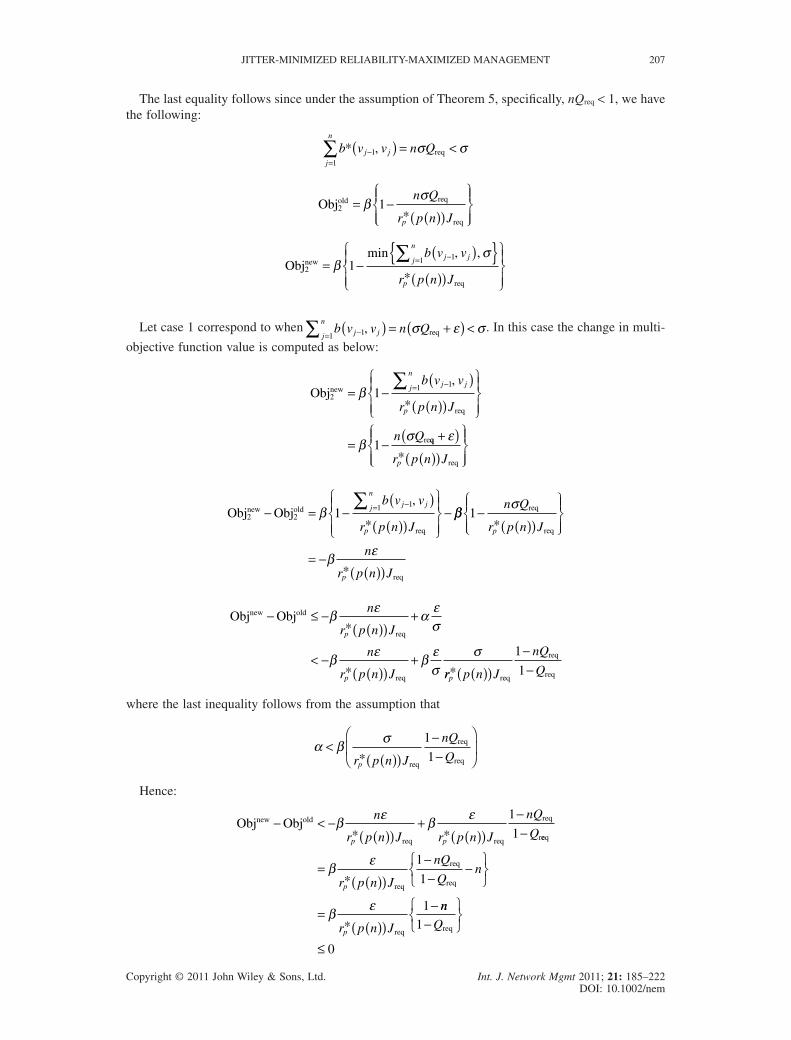
The last equality follows since under the assumption of Theorem 5, specifically, nQreq < 1, we havethe following:

b v v n Qj jj

n

* req−=

( ) = <∑ 11

, σ σ

Objold req

req

2 1= −( )( )

⎧⎨⎪

⎩⎪

⎫⎬⎪

⎭⎪β

σn Q

r p n Jp*

Objnew

req

2

111= −( ){ }

( )( )

⎧⎨⎪

⎩⎪

⎫⎬⎪

⎭⎪

−=∑β

σmin , ,

*

b v v

r p n J

j jj

n

p

Let case 1 correspond to when b v v n Qj jj

n

−=( ) = +( ) <∑ 11

, σ ε σreq . In this case the change in multi-

objective function value is computed as below:

Objnew

req

re

2

111

1

= −( )( )( )

⎧⎨⎪

⎩⎪

⎫⎬⎪

⎭⎪

= −

−=∑β

βσ

b v v

r p n J

n Q

j jj

n

p

,

*

qq

req

+( )( )( )

⎧⎨⎪

⎩⎪

⎫⎬⎪

⎭⎪

ε

r p n Jp*

Obj Objnew old

req

2 2

111− = −( )( )( )

⎧⎨⎪

⎩⎪

⎫⎬⎪

⎭⎪−

−=∑β

b v v

r p n J

j jj

n

p

,

*ββ

σ

β ε

1−( )( )

⎧⎨⎪

⎩⎪

⎫⎬⎪

⎭⎪

= −( )( )

n Q

r p n J

n

r p n J

p

p

req

req

req

*

*

Obj Objnew old

req

req

− ≤ −( )( )

+

< −( )( )

+

β ε α εσ

β ε β εσ

σ

n

r p n J

n

r p n J

p

p

*

* rr p n J

nQ

Qp* ( )( )

−−

req

req

req

1

1

where the last inequality follows from the assumption that

α β σ<( )( )

−−

⎛

⎝⎜

⎞

⎠⎟

r p n J

nQ

Qp* req

req

req

1

1

Hence:

Obj Objnew old

req req

req

r

− < −( )( )

+( )( )

−−

β ε β εn

r p n J r p n J

nQ

Qp p* *

1

1 eeq

req

req

req

req

=( )( )

−−

−⎧⎨⎩

⎫⎬⎭

=( )( )

−

β ε

β ε

r p n J

nQ

Qn

r p n J

p

p

*

*

1

1

1 nn

Q1

0

−⎧⎨⎩

⎫⎬⎭

≤

req



where the last inequality follows since n = 1, 2, . . . and 0 � Qreq < 1.

Case 2 corresponds to when b v v n Qj jj

n

−=( ) = +( ) >∑ 11

, σ ε σreq . In this case the change in multi-

objective function value is computed as below:

Objoldreq1 = αQ

Objnewreq1 1= +{ }α ε

σmin ,Q

max Obj Objnew oldreq1 1 1−{ } = −( )α Q

We will show that for any positive e which results in feasible solutions, the decrease in Obj2 will begreater than the increase in Obj1 under the assumptions of Theorem 5.

Obj*

old

req

r

2

111

1

= −( )

( )( )

⎧⎨⎪

⎩⎪

⎫⎬⎪

⎭⎪

= −

−=∑β

βσ

b v v

r p n J

n Q

j jj

n

p

,

*

eeq

reqr p n Jp* ( )( )

⎧⎨⎪

⎩⎪

⎫⎬⎪

⎭⎪

Objnew

req

2 1= −( )( )

⎧⎨⎪

⎩⎪

⎫⎬⎪

⎭⎪β σ

r p n Jp*

Obj Objnew old

req

req2 2 1 1− = −

( )( )

⎧⎨⎪

⎩⎪

⎫⎬⎪

⎭⎪− −β σ β

σ

r p n J

n Q

r p np p* * (( )( )

⎧⎨⎪

⎩⎪

⎫⎬⎪

⎭⎪

= −−( )( )( )

J

nQ

r p n Jp

req

req

req

βσ 1

*

Obj Objnew old req

req

req

r

− ≤ −−( )( )( )

+ −( )

< −−

βσ

α

βσ

11

1

nQ

r p n JQ

nQ

p*

eeq

req

req

req

( )( )( )

+−( )( )( )

=r p n J

nQ

r p n Jp p* *β

σ 1

0

where the last equality follows from the assumption that α β σ<( )( )

−−

⎛

⎝⎜

⎞

⎠⎟

r p n J

nQ

Qp* req

req

req

1

1. This con-

cludes the proof of Theorem 5. �


−−

⎛

⎝⎜

⎞

⎠⎟

r p n J

nQ

Qp* req

req

req

1

1, where 0 � Qreq < 1,

J r p n B v vp j jj

n

req * min , ,( )( ) < ( ){ }−=∑σ 11and nQreq � 1, then the optimal values of the buffers are

given by

b v v B v vJ r p n

nj j

j nj j

req p* −≤ ≤

−( ) = ( ) ( )( )⎧⎨⎪

⎩⎪

⎫⎬1

11, min min min , ,

* ⎪⎪

⎭⎪

⎧⎨⎪

⎩⎪

⎫⎬⎪

⎭⎪=

,

, , . . . , .

σ

for all j n1 2



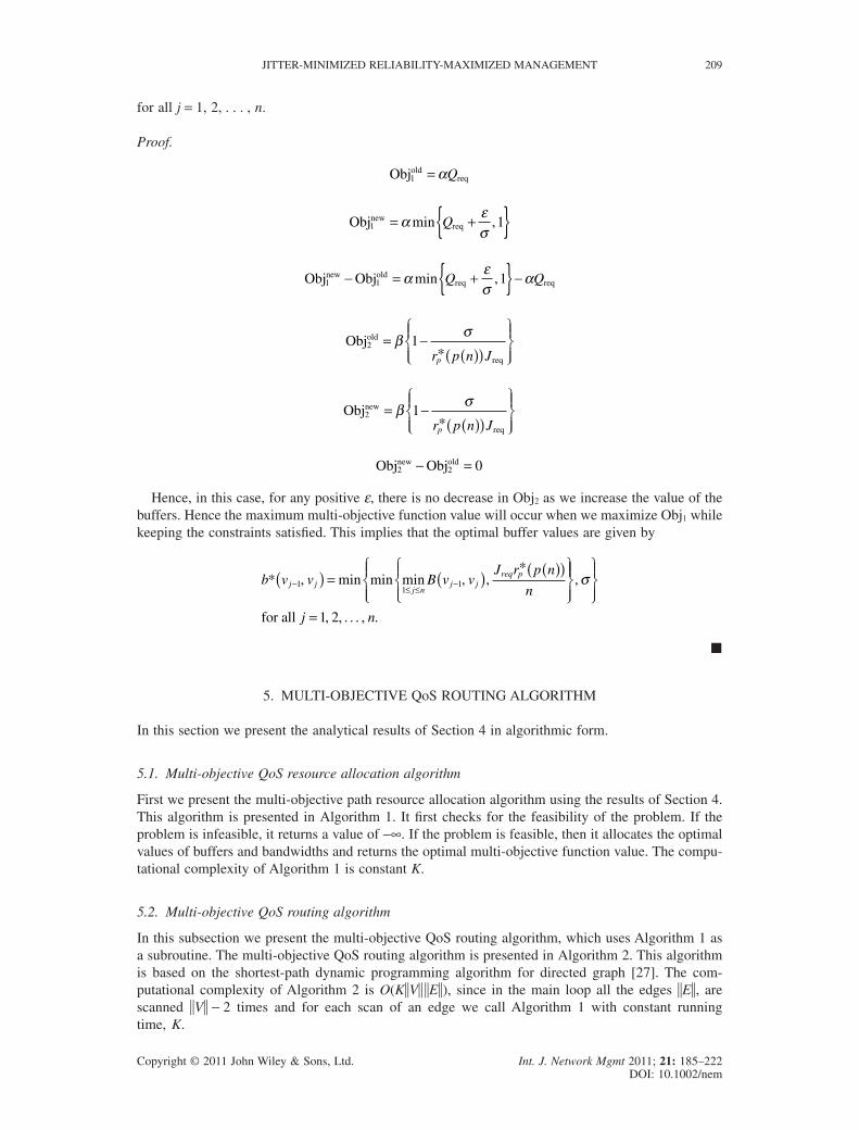
for all j = 1, 2, . . . , n.

Proof.

Objoldreq1 = αQ

Objnewreq1 1= +{ }α ε

σmin ,Q

Obj Objnew oldreq req1 1 1− = +{ }−α ε

σαmin ,Q Q

Objold

req

2 1= −( )( )

⎧⎨⎪

⎩⎪

⎫⎬⎪

⎭⎪β σ

r p n Jp*

Objnew

req

2 1= −( )( )

⎧⎨⎪

⎩⎪

⎫⎬⎪

⎭⎪β σ

r p n Jp*


Hence, in this case, for any positive e, there is no decrease in Obj2 as we increase the value of thebuffers. Hence the maximum multi-objective function value will occur when we maximize Obj1 whilekeeping the constraints satisfied. This implies that the optimal buffer values are given by

b v v B v vJ r p n

nj j

j nj j

req p* −≤ ≤

−( ) = ( ) ( )( )⎧⎨⎪

⎩⎪

⎫⎬1

11, min min min , ,

* ⎪⎪

⎭⎪

⎧⎨⎪

⎩⎪

⎫⎬⎪

⎭⎪=

,

, , . . . , .

σ

for all j n1 2

�

5. MULTI-OBJECTIVE QoS ROUTING ALGORITHM

In this section we present the analytical results of Section 4 in algorithmic form.

5.1. Multi-objective QoS resource allocation algorithm

First we present the multi-objective path resource allocation algorithm using the results of Section 4.This algorithm is presented in Algorithm 1. It first checks for the feasibility of the problem. If theproblem is infeasible, it returns a value of -•. If the problem is feasible, then it allocates the optimalvalues of buffers and bandwidths and returns the optimal multi-objective function value. The compu-tational complexity of Algorithm 1 is constant K.

5.2. Multi-objective QoS routing algorithm

In this subsection we present the multi-objective QoS routing algorithm, which uses Algorithm 1 asa subroutine. The multi-objective QoS routing algorithm is presented in Algorithm 2. This algorithmis based on the shortest-path dynamic programming algorithm for directed graph [27]. The com-putational complexity of Algorithm 2 is O(K�V� �E�), since in the main loop all the edges �E�, arescanned �V� - 2 times and for each scan of an edge we call Algorithm 1 with constant runningtime, K.



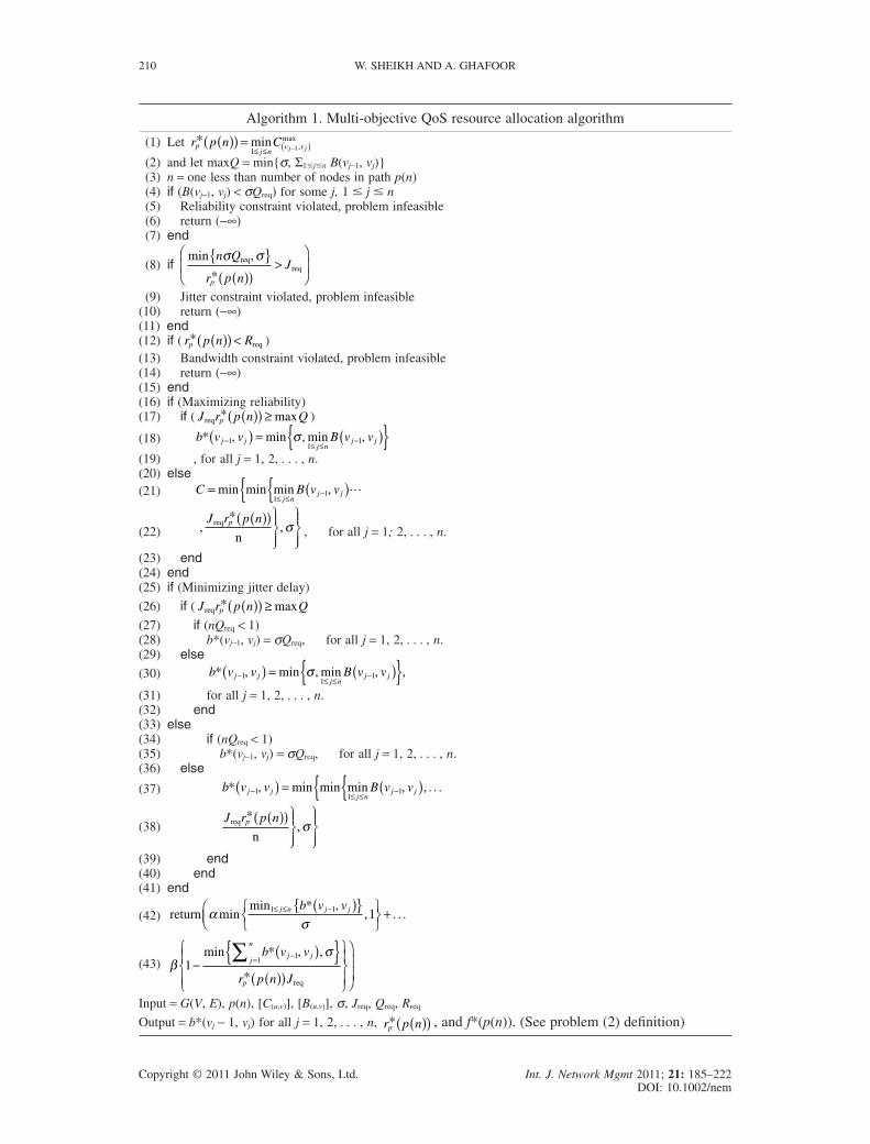
Algorithm 1. Multi-objective QoS resource allocation algorithm

(1) Let r p n Cpj n

v vj j* min ,

max( )( ) =≤ ≤ ( )−1 1

(2) and let maxQ = min{s, S1�j�n B(vj-1, vj)}(3) n = one less than number of nodes in path p(n)(4) if (B(vj-1, vj) < sQreq) for some j, 1 � j � n(5) Reliability constraint violated, problem infeasible(6) return (-•)(7) end

(8) ifmin ,

*

n Q

r p nJ

p

σ σreqreq

{ }( )( )

>⎛

⎝⎜

⎞

⎠⎟

(9) Jitter constraint violated, problem infeasible(10) return (-•)(11) end(12) if ( r p n Rp* ( )( ) < req )(13) Bandwidth constraint violated, problem infeasible(14) return (-•)(15) end(16) if (Maximizing reliability)(17) if ( J r p n Qpreq * max( )( ) ≥ )

(18) b v v B v vj jj n

j j* −≤ ≤

−( ) = ( ){ }11

1, min , min ,σ(19) , for all j = 1, 2, . . . , n.(20) else(21) C B v v

j nj j= ( ){{ ≤ ≤−min min min ,

11 �

(22) ,*

,J r p npreq

n

( )( ) ⎫⎬⎪

⎭⎪

⎫⎬⎪

⎭⎪σ , for all j = 1; 2, . . . , n.

(23) end(24) end(25) if (Minimizing jitter delay)

(26) if ( J r p n Qpreq * max( )( ) ≥(27) if (nQreq < 1)(28) b*(vj-1, vj) = sQreq, for all j = 1, 2, . . . , n.(29) else(30) b v v B v vj j

j nj j* −

≤ ≤−( ) = ( ){ }1

11, min , min , ,σ

(31) for all j = 1, 2, . . . , n.(32) end(33) else(34) if (nQreq < 1)(35) b*(vj-1, vj) = sQreq, for all j = 1, 2, . . . , n.(36) else

(37) b v v B v vj jj n

j j* −≤ ≤

−( ) = ( ){{11

1, min min min , , . . .

(38)J r p npreq

n

*,

( )( ) ⎫⎬⎪

⎭⎪

⎫⎬⎪

⎭⎪σ

(39) end(40) end(41) end

(42) return*

ασ

minmin ,

, . . .1 1 1≤ ≤ −( ){ }⎧⎨⎩

⎫⎬⎭+⎛

⎝⎜j n j jb v v

(43) βσ

11

1−( ){ }

( )( )

⎧⎨⎪

⎩⎪

⎫⎬⎪

⎭⎪

⎞

⎠⎟⎟

−=∑min , ,

*

b v v

r p n J

j jj

n

p

*

req

Input = G(V, E), p(n), [C(u,v)], [B(u,v)], s, Jreq, Qreq, Rreq

Output = b*(vj - 1, vj) for all j = 1, 2, . . . , n, r p np* ( )( ) , and f*(p(n)). (See problem (2) definition)



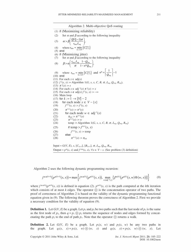
Algorithm 2 uses the following dynamic programming recursion:

f p s x f p s xk k k k

w x** * ** *

adj

+( ) +( ) ( ) ( )∈ ( )

( )( ) = ( )( )−

1 1

1, max , , max ff p s w w xk k* *( ) ( ) ( )⊕( )( ){ }{ }, , (9)

where f **(k)(p*(k)(s, x)) is defined in equation (2). p*(k)(s, x) is the path computed at the kth iterationwhich consists of at most k edges. The operator � is the concatenation operator of two paths. Theproof of correctness of Algorithm 2 is based on the validity of the dynamic programming functionalequation given in (9). The following theorem proves the correctness of Algorithm 2. First we providea necessary condition for the validity of equation (9).

Definition 1. Let G(V, E) be a graph. Let p1 and p2 be two paths such that the last node of p1 is the sameas the first node of p2, then q = p1 � p2 returns the sequence of nodes and edges formed by concat-enating the path p2 to the end of path p1. Note that the operator � returns a walk.

Definition 2. Let G(V, E) be a graph. Let p1(s, w) and p2(s, w) be any two paths inthe graph. Let q1(s, x) = p1(s, w) � (w, x) and q2(s, x) = p2(s, w) � (w, x). Let

Algorithm 2. Multi-objective QoS routing

(1) if (Maximizing reliability)(2) Set a and b according to the following inequality

(3) α β σ> −( )⎛⎝⎜

⎞⎠⎟

V

r J

1

min

,req

(4) where r Cu v E

u vmin,

,maxmin= { }

( )∈ ( )(5) end(6) if (Minimizing jitter)(7) Set a and b according to the following inequality

(8) β ασ

>−

−⎛⎝⎜

⎞⎠⎟

r J Q

n Qmax ,req req

req*

1

1

(9) where r Cu v E

u vmax,

,maxmin= { }

( )∈ ( ) and nQ

* =⎡

⎢⎢

⎤

⎥⎥ −

11

req(10) end(11) For each x ∈ adj(s)(12) f 1(s, x) := Algorithm 1(G, s, x, C, B, s, Jreq, Qreq, Rreq),(13) p 1(x) := s(14) For each x ∈ adj-1(s) p 1(x) := x(15) For each x ∉ adj(s) f 1(s, x) := -•(16) Main loop(17) for k := 1 → �V� - 2(18) for each node x ∈ V - {s}(19) f k+1(s, x) := f k(s, x)

(20) p k+1(x) := p k(x)(21) for each node w ∈ adj-1(x)(22) pold := p k+1(x)(23) p k+1(x) := w(24) temp := Algorithm 1(G, s, x, C, B, s, Jreq, Qreq, Rreq)

(25) if temp > f k+1(s, x)(26) f k+1(s, x) := temp(27) else(28) p k+1(x) := pold

Input = G(V, E), s, [C(u,v)], [B(u,v)], s, Jreq, Qreq, Rreq

Output = p*(s, x) and f **(s, x), "x ∈ V - s. (See problem (3) definition)



Q pJ p

JQ p

J p

Jp

pp

p**

**

11

221 1( ) + −

( )⎧⎨⎪

⎩⎪

⎫⎬⎪

⎭⎪≥ ( ) + −

( )⎧⎨⎪

⎩⎪req req

⎫⎫⎬⎪

⎭⎪. We say that the paths p1 and p2 satisfy the monoto-

nicity condition if the above inequality implies Q qJ q

JQ q

J q

Jp

pp

p**

**

11

221 1( ) + −

( )⎧⎨⎪

⎩⎪

⎫⎬⎪

⎭⎪≥ ( ) + −

( )⎧⎨⎪

⎩⎪req req

⎫⎫⎬⎪

⎭⎪for all

edges (w, x) such that the first inequality holds true. We say that a graph satisfies the monotonicitycondition if the above definition holds for any pair of paths in the graph which satisfy the firstinequality.

Note that a path consisting of GPS routers satisfies the monotonicity condition.

Theorem 7. Given G(V, E), s, [C(u,v)], [B(u,v)], s, Jreq, Qreq, Rreq. Assume that the monotonicity conditionis satisfied. Then at the termination of Algorithm 2 the following statements are true:

1. f (�V�-1)(s, x) = -• for every node x ∈ V such that x is not reachable from the source node s.2. p (�V�-1)(s, x) = f for every x ∈ V such that x is not reachable from s.3. f (�V�-1)(s, x) = f **(s, x) for every node x ∈ V such that x is reachable from s where f **(s, x) is

defined in equation (3).4. The graph Gp = (V, Ep) such that Ep = {(p�V�-1(x), x) : p�V�-1 � f} contains the path p*(s, x) for

every node x ∈ V if x is reachable from s. The path p*(s, x) is defined in equation (3).

Proof. Proof of the theorem is by induction on the variable k of iteration in the main loop of Algorithm2. The induction basis corresponds to when k = 1. In this case the path p*(1)(s, x) consists of a singleedge for all x ∈ adj(s). In the initialization loop of Algorithm 2, Algorithm 1 is applied to each edge(s, x) for x ∈ adj(s). If the edge (s, x) is a feasible path from s to x, then f (1)(s, x) = f (1)**(s, x) andp 1(x) = s. If the edge is infeasible then Algorithm 1 returns -• and p 1(s, x) = f.

The induction hypothesis is given as follows. At the end of the kth iteration, for every node x ∈ Vsuch that there exists a path from s to x consisting of at most k edges, f (k)(s, x) = f (k)**. Let p*(k)(s, x)be the path that produces f (k)**. Then at the end of kth iteration p k(x) can be traced back to the sourcenode s to provide p*(k)(s, x). If for some node x there exists no path from s to x consisting of at mostk edges, then f k(s, x) = -• and p k(x) = f.

Using the above induction hypothesis we will show that for every node x that can be reachedfrom s in at most k + 1 edges, f (k+1)(s, x) = f **(k+1)(s, x). Recall that the recursive equation to computef (k+1)(s, x) is given as follows:

f p s x f p s x fk k k k

w x

k+( ) + ( ) ( )∈ ( )

( )( )( ) = ( )( )−

1 1

1, max , , max** * *

adjpp s w w xk*( ) ( )⊕( )( ){ }{ }, , (10)

Recall that f s x f p s xkp s x** **+( )( )∈ ( )( ) = ( )( ){ }+( )

11, max ,, * ,P s xk . There are two cases to

consider. Firstly, f p s x f p s w w xk kw x

k k** * * *adj( ) ( )

∈ ( )( ) ( )( )( ) ≥ ( )⊕( )( ){ }−, max , ,1 . In this case

Table 2. Simulation parameters.

Symbol Explanation Value Units

l Intensity of Poisson process for Waxman topology 0.6g Link probability parameter for Waxman topology 3d Link probability parameter for Waxman topology 0.1N Number of nodes 60s Source node 3s Bucket size, leaky bucket parameter Mbytes/sr Average traffic rate, leaky bucket parameter 100 Mbytes/sJreq Required jitter delay SecondsQreq Required reliabilityRreq Required bandwidth 100 Mbytes/sB Maximum physical buffer available MbytesC Maximum available link capacity Mbytes/s



f (k+1)(s, x) = f **(k)(p*(k)(s, x)) = f **(k+1)(s, x). This follows from the induction hypothesis, sincef **(k)(s, x) is the optimal objective function value corresponding to the optimal path from s to xconsisting of at most k edges. In this case the optimal path is the same as constructed by p k(x). In thesecond case f p s x f p s w w xk k

w xk k** * * *adj

( ) ( )∈ ( )

( ) ( )( )( ) < ( )⊕( )( ){ }−, max , ,1 . Any path pk+1(s, x) can be

represented as pk+1(s, x) = pk(s, x) � (w, x). From the monotonicity condition it follows that

max , , ,w xk k kf p s w w x f s x∈ ( )( ) ( ) +( )

− ( )⊕( )( ){ } = ( )adj * * **11 . pk+1(x) can be traced back to the source node

s to provide p*(k+1)(s, x) by appending the edge (w*, x) to the path p*(k)(s, w), which is available fromthe induction hypothesis. If there exists no path from s to x consisting of at most k + 1 edges, then thevalue of f**(k+1)(s, x) stays the same as it was initialized with, i.e., -•. The value of the parent node alsodoes not change in Algorithm 2; hence in this case p k+1(x) = f. Since a path, containing no cycles, froms to x can consist of at most V - 1 edges, at the termination of the algorithm the statement of Theorem7 is true. The reason we do not have to consider path-containing cycles is because including a cycle ona path does not increase the objective function value. �

6. SIMULATION RESULTS

This section presents the simulation results by studying the effects of various parameters, such asmaximum physical buffer size B, maximum link bandwidth C, required reliability Qreq, required jitterdelay Jreq and bucket size s [4,22,24,28], on the multi-objective QoS routing algorithm. The objective

Figure 1. Effect of maximum physical buffer size, B, on reliability of paths, Qp: s = 200 MB,r = 100 MB/s, Qreq = 0.01, Jreq = 5 s, Rreq = 100 MB/s, C = 200 MB/s. (a) Maximum reliability of all

paths; (b) minimum reliability of all paths; (c) average reliability; (d) number of feasible paths.



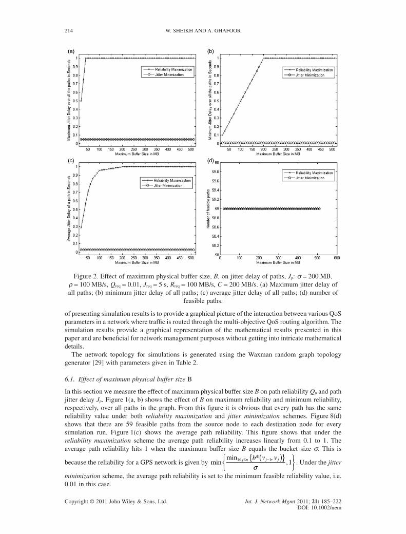
of presenting simulation results is to provide a graphical picture of the interaction between various QoSparameters in a network where traffic is routed through the multi-objective QoS routing algorithm. Thesimulation results provide a graphical representation of the mathematical results presented in thispaper and are beneficial for network management purposes without getting into intricate mathematicaldetails.

The network topology for simulations is generated using the Waxman random graph topologygenerator [29] with parameters given in Table 2.

6.1. Effect of maximum physical buffer size B

In this section we measure the effect of maximum physical buffer size B on path reliability Qp and pathjitter delay Jp. Figure 1(a, b) shows the effect of B on maximum reliability and minimum reliability,respectively, over all paths in the graph. From this figure it is obvious that every path has the samereliability value under both reliability maximization and jitter minimization schemes. Figure 8(d)shows that there are 59 feasible paths from the source node to each destination node for everysimulation run. Figure 1(c) shows the average path reliability. This figure shows that under thereliability maximization scheme the average path reliability increases linearly from 0.1 to 1. Theaverage path reliability hits 1 when the maximum buffer size B equals the bucket size s. This is

because the reliability for a GPS network is given by minmin ,

,1 1 1≤ ≤ −( ){ }⎧⎨⎩

⎫⎬⎭

j n j jb v v*

σ. Under the jitter

minimization scheme, the average path reliability is set to the minimum feasible reliability value, i.e.0.01 in this case.

Figure 2. Effect of maximum physical buffer size, B, on jitter delay of paths, Jp: s = 200 MB,r = 100 MB/s, Qreq = 0.01, Jreq = 5 s, Rreq = 100 MB/s, C = 200 MB/s. (a) Maximum jitter delay ofall paths; (b) minimum jitter delay of all paths; (c) average jitter delay of all paths; (d) number of

feasible paths.



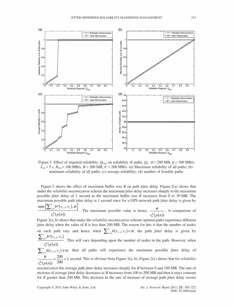
Figure 2 shows the effect of maximum buffer size B on path jitter delay. Figure 2(a) shows thatunder the reliability maximization scheme the maximum jitter delay increases sharply to the maximumpossible jitter delay of 1 second as the maximum buffer size B increases from 0 to 50 MB. Themaximum possible path jitter delay is 1 second since for a GPS network path jitter delay is given by

min , ,

*

b v v

r p n

j jj

n

p

* −=( ){ }( )( )

∑ 11σ

. The maximum possible value is hence σ

r p np* ( )( ). A comparison of

Figure 2(a, b) shows that under the reliability maximization scheme optimal paths experience differentjitter delay when the value of B is less than 200 MB. The reason for this is that the number of nodes

on each path vary and hence when b v vj jj

n

−=( ) <∑ 11

, σ , the path jitter delay is given by

b v v

r p n

j jj

n

p

* −=( )( )( )

∑ 11,

*. This will vary depending upon the number of nodes in the path. However, when

b v vj jj

n

−=( ) ≥∑ 11

, σ , then all paths will experience the maximum possible jitter delay of

σ

r p np* ( )( )= =200

2001 second. This is obvious from Figure 2(a, b). Figure 2(c) shows that for reliability

maximization the average path jitter delay increases sharply for B between 0 and 100 MB. The rate ofincrease of average jitter delay decreases as B increases from 100 to 200 MB and then it stays constantfor B greater than 200 MB. This decrease in the rate of increase of average path jitter delay occurs

Figure 3. Effect of required reliability, Qreq, on reliability of paths, Qp: s = 200 MB, r = 100 MB/s,Jreq = 5 s, Rreq = 100 MB/s, B = 200 MB, C = 200 MB/s. (a) Maximum reliability of all paths; (b)

minimum reliability of all paths; (c) average reliability; (d) number of feasible paths.



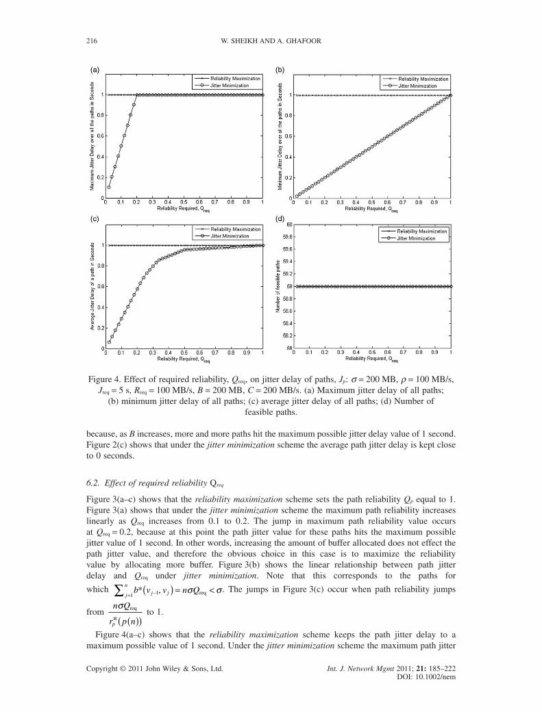
because, as B increases, more and more paths hit the maximum possible jitter delay value of 1 second.Figure 2(c) shows that under the jitter minimization scheme the average path jitter delay is kept closeto 0 seconds.

6.2. Effect of required reliability Qreq

Figure 3(a–c) shows that the reliability maximization scheme sets the path reliability Qp equal to 1.Figure 3(a) shows that under the jitter minimization scheme the maximum path reliability increaseslinearly as Qreq increases from 0.1 to 0.2. The jump in maximum path reliability value occursat Qreq = 0.2, because at this point the path jitter value for these paths hits the maximum possiblejitter value of 1 second. In other words, increasing the amount of buffer allocated does not effect thepath jitter value, and therefore the obvious choice in this case is to maximize the reliabilityvalue by allocating more buffer. Figure 3(b) shows the linear relationship between path jitterdelay and Qreq under jitter minimization. Note that this corresponds to the paths for

which b v v n Qj jj

n* req−=( ) = <∑ 11

, σ σ . The jumps in Figure 3(c) occur when path reliability jumps

fromn Q

r p np

σ req

* ( )( )to 1.

Figure 4(a–c) shows that the reliability maximization scheme keeps the path jitter delay to amaximum possible value of 1 second. Under the jitter minimization scheme the maximum path jitter

Figure 4. Effect of required reliability, Qreq, on jitter delay of paths, Jp: s = 200 MB, r = 100 MB/s,Jreq = 5 s, Rreq = 100 MB/s, B = 200 MB, C = 200 MB/s. (a) Maximum jitter delay of all paths;

(b) minimum jitter delay of all paths; (c) average jitter delay of all paths; (d) Number offeasible paths.



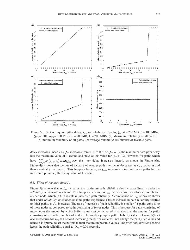
delay increases linearly as Qreq increases from 0.01 to 0.2. At Qreq = 0.2 the maximum path jitter delayhits the maximum value of 1 second and stays at this value for Qreq > 0.2. However, for paths which

have b v v n Qj jj

n* req−=( ) = <∑ 11

, σ σ , the jitter delay increases linearly as shown in Figure 4(b).

Figure 4(c) shows that the rate of increase of average path jitter delay decreases as Qreq increases andthen eventually becomes 0. This happens because, as Qreq increases, more and more paths hit themaximum possible jitter delay value of 1 second.

6.3. Effect of required jitter Jreq

Figure 5(a) shows that as Jreq increases, the maximum path reliability also increases linearly under thereliability maximization scheme. This happens because, as Jreq increases, we can allocate more bufferat each node, which in turn results in increased path reliability. A comparison of Figure 5(a, b) showsthat under reliability maximization some paths experience a faster increase in path reliability relativeto other paths, as Jreq increases. The rate of increase of path reliability is smaller for paths consistingof more nodes as compared to paths consisting of fewer nodes. This is because for paths consisting ofmore nodes the amount by which buffer values can be increased is smaller than the amount for pathsconsisting of a smaller number of nodes. The sudden jump in path reliability value in Figure 5(b, c)occurs because for Jreq � 1 second increasing the buffer value will not change the path jitter value andhence it is optimal to set the buffers to their maximum possible values. The jitter minimization schemekeeps the path reliability equal to Qreq = 0.01 seconds.

Figure 5. Effect of required jitter delay, Jreq, on reliability of paths, Qp: s = 200 MB, r = 100 MB/s,Qreq = 0.01, Rreq = 100 MB/s, B = 200 MB, C = 200 MB/s. (a) Maximum reliability of all paths;

(b) minimum reliability of all paths; (c) average reliability; (d) number of feasible paths.



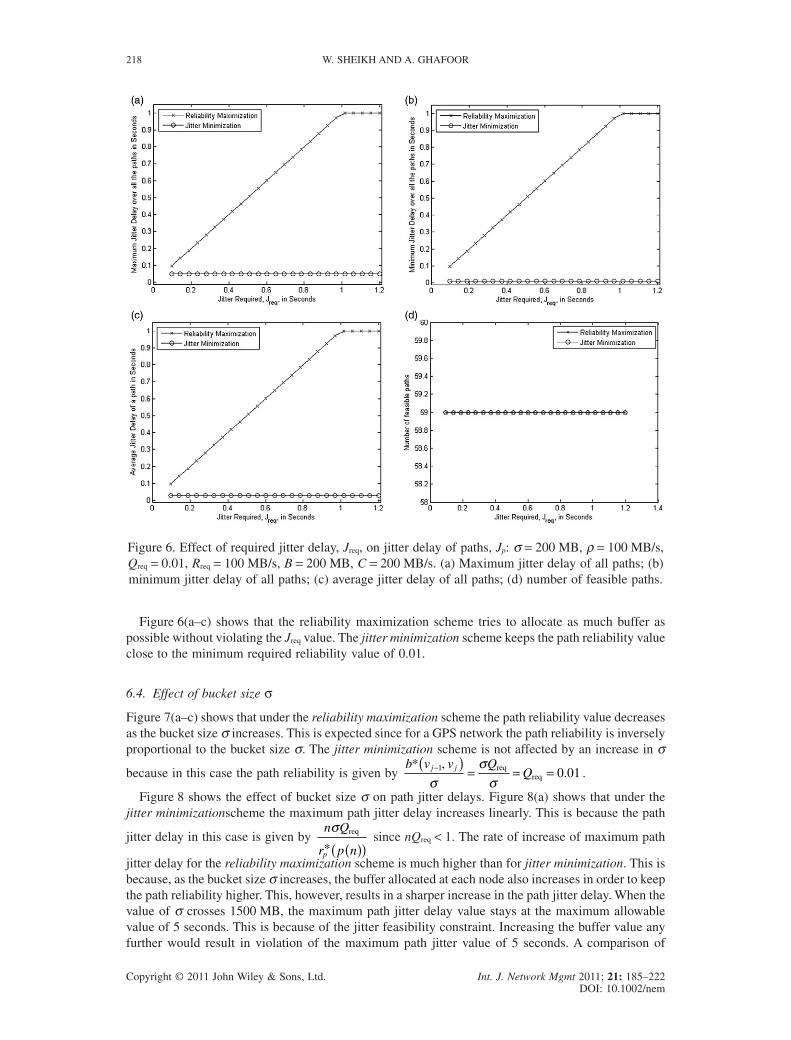
Figure 6(a–c) shows that the reliability maximization scheme tries to allocate as much buffer aspossible without violating the Jreq value. The jitter minimization scheme keeps the path reliability valueclose to the minimum required reliability value of 0.01.

6.4. Effect of bucket size s

Figure 7(a–c) shows that under the reliability maximization scheme the path reliability value decreasesas the bucket size s increases. This is expected since for a GPS network the path reliability is inverselyproportional to the bucket size s. The jitter minimization scheme is not affected by an increase in s

because in this case the path reliability is given byb v v Q

Qj j* reqreq

−( ) = = =1 0 01,

.σ

σσ

.

Figure 8 shows the effect of bucket size s on path jitter delays. Figure 8(a) shows that under thejitter minimizationscheme the maximum path jitter delay increases linearly. This is because the path

jitter delay in this case is given byn Q

r p np

σ req

* ( )( )since nQreq < 1. The rate of increase of maximum path

jitter delay for the reliability maximization scheme is much higher than for jitter minimization. This isbecause, as the bucket size s increases, the buffer allocated at each node also increases in order to keepthe path reliability higher. This, however, results in a sharper increase in the path jitter delay. When thevalue of s crosses 1500 MB, the maximum path jitter delay value stays at the maximum allowablevalue of 5 seconds. This is because of the jitter feasibility constraint. Increasing the buffer value anyfurther would result in violation of the maximum path jitter value of 5 seconds. A comparison of

Figure 6. Effect of required jitter delay, Jreq, on jitter delay of paths, Jp: s = 200 MB, r = 100 MB/s,Qreq = 0.01, Rreq = 100 MB/s, B = 200 MB, C = 200 MB/s. (a) Maximum jitter delay of all paths; (b)minimum jitter delay of all paths; (c) average jitter delay of all paths; (d) number of feasible paths.



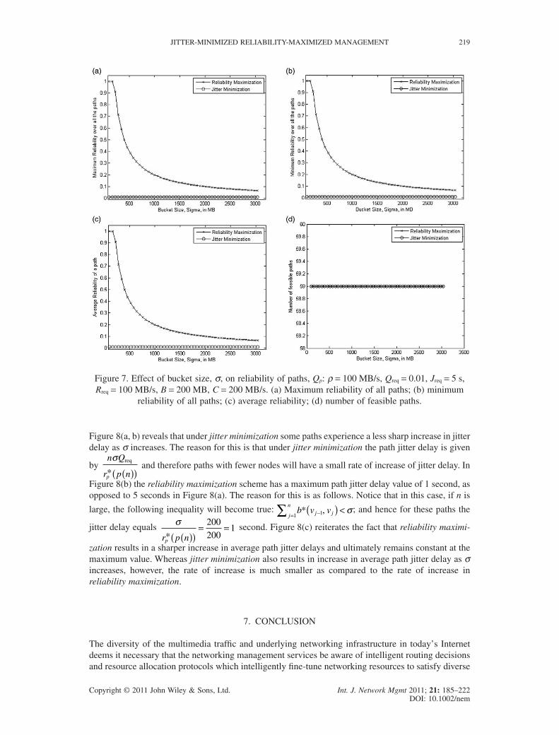
Figure 8(a, b) reveals that under jitter minimization some paths experience a less sharp increase in jitterdelay as s increases. The reason for this is that under jitter minimization the path jitter delay is given

byn Q

r p np

σ req

* ( )( )and therefore paths with fewer nodes will have a small rate of increase of jitter delay. In

Figure 8(b) the reliability maximization scheme has a maximum path jitter delay value of 1 second, asopposed to 5 seconds in Figure 8(a). The reason for this is as follows. Notice that in this case, if n is

large, the following inequality will become true: b v vj jj

n* −=( ) <∑ 11

, σ; and hence for these paths the

jitter delay equals σ

r p np* ( )( )= =200

2001 second. Figure 8(c) reiterates the fact that reliability maximi-

zation results in a sharper increase in average path jitter delays and ultimately remains constant at themaximum value. Whereas jitter minimization also results in increase in average path jitter delay as sincreases, however, the rate of increase is much smaller as compared to the rate of increase inreliability maximization.

7. CONCLUSION

The diversity of the multimedia traffic and underlying networking infrastructure in today’s Internetdeems it necessary that the networking management services be aware of intelligent routing decisionsand resource allocation protocols which intelligently fine-tune networking resources to satisfy diverse

Figure 7. Effect of bucket size, s, on reliability of paths, Qp: r = 100 MB/s, Qreq = 0.01, Jreq = 5 s,Rreq = 100 MB/s, B = 200 MB, C = 200 MB/s. (a) Maximum reliability of all paths; (b) minimum

reliability of all paths; (c) average reliability; (d) number of feasible paths.



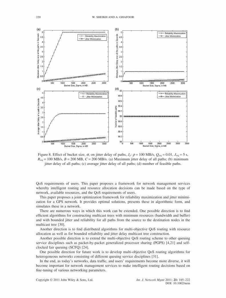
QoS requirements of users. This paper proposes a framework for network management serviceswhereby intelligent routing and resource allocation decisions can be made based on the type ofnetwork, available resources, and the QoS requirements of users.

This paper proposes a joint optimization framework for reliability maximization and jitter minimi-zation for a GPS network. It provides optimal solutions, presents these in algorithmic form, andsimulates these in a network.

There are numerous ways in which this work can be extended. One possible direction is to findefficient algorithms for constructing multicast trees with minimum resources (bandwidth and buffer)and with bounded jitter and reliability for all paths from the source to the destination nodes in themulticast tree [30].

Another direction is to find distributed algorithms for multi-objective QoS routing with resourceallocation as well as for bounded reliability and jitter delay multicast tree construction.

Another possible direction is to extend the multi-objective QoS routing scheme to other queuingservice disciplines such as packet-by-packet generalized processor sharing (PGPS) [4,21] and self-clocked fair queuing (SCFQ) [24].

One possible direction for future work is to develop multi-objective QoS routing algorithms forheterogeneous networks consisting of different queuing service disciplines [31].

In the end, as today’s networks, data traffic, and users’ requirements become more diverse, it willbecome important for network management services to make intelligent routing decisions based onfine-tuning of various networking parameters.

Figure 8. Effect of bucket size, s, on jitter delay of paths, Jp: r = 100 MB/s, Qreq = 0.01, Jreq = 5 s,Rreq = 100 MB/s, B = 200 MB, C = 200 MB/s. (a) Maximum jitter delay of all paths; (b) minimum

jitter delay of all paths; (c) average jitter delay of all paths; (d) number of feasible paths.



REFERENCES

1. Joseph CA, Muralidhar K. Integrated network management in an enterprise environment. IEEE Network Magazine 1990;4(4): 7–13.

2. Baqai S, Khan MF, Ghafoor A. Handbook of Multimedia Information Management, Grosky W, Jain R, Mehrotra R (eds).Prentice-Hall: Englewood Cliffs, NJ, 1997.

3. Demers A, Keshav S, Shenker S. Analysis and simulation of a fair queueing algorithm. Internetworking, Research andExperience 1990; 1(1): 3–26.

4. Parekh AK, Gallager RG. A generalized processor sharing approach to flow control in integrated services networks: thesingle-node case. IEEE/ACM Transactions on Networking 1993; 1(3): 344–357.

5. Bashandy AR, Chong EKP, Ghafoor A. Generalized quality-of-service routing with resource allocation. IEEE Journal onSelected Areas in Communications 2005; 23(2): 450–463.

6. Chen S, Nahrstedt K. An overview of quality-of-service routing for the next generation high-speed networks: problems andsolutions. IEEE Network 1998; 12: 64–79.

7. Orda A. Routing with end to end qos guarantees in broadband networks. In IEEE INFOCOM, Vol. 1, April 1998; 27–34.8. Cidon I, Rom R, Shavitt Y. Multi-path routing combined with resource reservation. In IEEE INFOCOM, April 1997;

92–100.9. Ma Q, Steenkiste P. Quality of service routing for traffic with performance guarantees. In International Workshop on

Quality of Service ’97 (IWQOS’97), 1997.10. Ma Q, Steenkiste P. Supporting dynamic inter-class resource sharing: a multi-class QoS routing algorithm. In IEEE

INFOCOM, Vol. 1, March 1999; 649–660.11. Orda A, Sprinnston A. Percomputation schemes for QoS routing. IEEE/ACM Transactions on Networking 2003; 11(4):

578–591.12. Sobrinho JL. Algebra and algorithms for qos path computation and hop-by-hop routing in the internet. IEEE/ACM

Transactions on Networking 2002; 10(4): 541–592.13. Yuan X. Heuristic algorithms for multiconstrained quality-of-service routing. IEEE/ACM Transactions on Networking

2002; 10(2): 244–256.14. Korkmaz T, Kruz M. Multi-constrained optimal path selection. In IEEE INFOCOM, Vol. 2, March 2001; 834–843.15. Jaffe JM. Algorithms for finding paths with multiple constraints. Networks 1984; 14(1): 95–116.16. Salama HF, Reeves DR, Viniotis Y. A distributed algorithm for delay-constrained unicast routing. In IEEE INFOCOM,

April 1997; 84–91.17. Vogel R, Herrtwich RG, Kalfa W, Wittig H, Wolf LC. Qos-based routing of multimedia streams in computer networks.

IEEE Journal on Selected Areas in Communications 1996; 14(7): 1235–1244.18. Wang Z, Crowcroft J. Quality-of-service routing for supporting multimedia applications. IEEE Journal on Selected Areas

in Communications 1996; 14(7): 1228–1234.19. Chen S, Nahrstedt K. On finding multi-constrained paths. In IEEE ICC, June 1998.20. Lin X, Shroff NB. An optimization-based approach for QoS routing in high-bandwidth networks. IEEE/ACM Transactions

on Networking 2006; 16(6): 1348–1361.21. Parekh AK, Gallager RG. A generalized processor sharing approach to flow control in integrated services networks: the

multile-node case. IEEE/ACM Transactions on Networking 1994; 2(2): 137–150.22. Bennett JCR, Zhang H. WF2Q: worst-case fair weighted fair queuing. In IEEE INFOCOM, 1996; 120–128.23. Figueira NR, Pasqual J. An upper bound on the delay for the VirtualClock service discipline. IEEE/ACM Transactions on

Networking 1995; 3(4): 399–408.24. Golestani SJ. A self clocked fair queuing scheme for broadband applications. In IEEE INFOCOM, June 1994; 636–646.25. Zhang H. Service disciplines for guaranteed performance service in packet switching networks. Proceedings of the IEEE

1995; 83(10): 1373–1396.26. Turner J. New directions in communication, or which way to the information age. IEEE Communication Magazine 1986;

24: 8–15.27. Bellman R. On a routing problem. Quarterly of Applied Mathematics 1958; 16(1): 87–90.28. Cruz RL. A calculus for network delay. Part I. Network elements in isolation. IEEE Transactions on Information Theory

1991; 37: 114–131.29. Waxman BM. Routing of multipoint connections. IEEE Journal on Selected Areas in Communications 1988; 6(9):

1617–-1622.30. Sheikh W, Ghafoor A. A combined approach for qos based multicast routing and resource allocation. In IEEE ICC, May

2005; 136–142.31. Sheikh W, Ghafoor A. Quality-of-service routing in heterogeneous networks with optimal buffer and bandwidth allocation.

In IEEE ICC, 2007.

AUTHORS’ BIOGRAPHIES

Waseem Sheikh received his PhD and MS in electrical and computer engineering from Purdue University, WestLafayette, Indiana, USA, in 2007 and 2002 respectively. He received his BS in electronics engineering fromGhulam Ishaq Khan Institute of Engineering and Technology, Pakistan, in 2000. His research interests includeoptimization techniques in computer networks.



Arif Ghafoor is currently a professor in the School of Electrical and Computer Engineering at Purdue University,West Lafayette, Indiana, USA, and is the Director of Distributed Multimedia Systems Laboratory. He has beenactively engaged in research areas related to multimedia systems, information security, and parallel and distributedcomputing. He has published over 150 technical papers in leading journals and conferences. Dr Ghafoor hasserved on the editorial boards of various journals including ACM/Springer Multimedia Systems Journal, Journalof Parallel and Distributed Databases, and International Journal on Computer Networks. He has served as aguest/co-guest editor for various special issues of numerous journals, including ACM/Springer MultimediaSystems Journal, Journal of Parallel and Distributed Computing, International Journal on Multimedia Tools andApplications, IEEE Journal on Selected Areas in Communications, and IEEE Transactions on Knowledge andData Engineering. He has co-edited a book entitled Multimedia Document Systems in Perspectives and hasco-authored a book entitled Semantic Models for Multimedia Database Searching and Browsing″ (KluwerAcademic Publishers, 2000). Dr Ghafoor is a Fellow of the IEEE. He has received the IEEE Computer Society2000 Technical Achievement Award for his research contributions in the area of multimedia systems.



Documents

Jitter-minimized reliability-maximized management of networks