Jim Tørresen - uio.no · Jim Tørresen This Lecture 1. ... think, learn, understand language, ++ ... Minsky and Papert prove limitations of Perceptron 1970s

23.09.15

1

INF3490 - Biologically inspired computing

Lecture 5: 21 September 2015 Intro to machine learning and single-layer neural networks

Jim Tørresen

This Lecture

1.  Introduction to learning/classification

2.  Biological neuron

3.  Perceptron and artificial neural networks

23 September 2015 2

Things You Might Be Interested In Learning from Data The world is driven by data.

•  Germany’s climate research centre generates 10 petabytes per year •  Google processes 24 petabytes per day (2009, 1000 Terabytes) •  The Large Hadron Collider produces 60 gigabytes per minute (~12

DVDs) •  There are over 50m credit card transactions a day in the US alone.

23.09.15

2

Big Data: If Data Had Mass, the Earth Would Be A Black Hole

•  Around the world, computers capture and store terabytes of data everyday.

•  Science has also taken advantage of the ability of computers to store massive amount of data.

•  The size and complexity of these data sets means that humans are unable to extract useful information from them.

23 September 2015 5

High-dimensional data

23 September 2015 6

A set of data points as numerical values as points plotted on a graph. It is easier for us to visualize data than to see it in a table, but if the data has more than three dimensions, we can’t view it all at once.

High-dimensional data

23 September 2015 7

Two views of the same two wind turbines (Te Apiti wind farm, Ashhurst, New Zealand) taken at an angle of about 300 to each other. The two-dimensional projections of three-dimensional objects hide information.

23 September 2015 8

Machine Learning

•  Ever since computers were invented, we have wondered whether they might be made to learn.

•  The ability of a program to learn from experience — that is, to modify its execution on the basis of newly acquired information.

•  Machine learning is about automatically extracting relevant information from data and applying it to analyze new data.

23.09.15

3

Idea Behind

•  Humans can: –  sense: see, hear, feel, ++ –  reason: think, learn, understand language, ++ –  respond: move, speak, act ++

•  Artificial Intelligence aims to reproduce these capabilities.

•  Machine Learning is one part of Artificial Intelligence.

23 September 2015 9

Characteristics of ML

•  Typically used for classification tasks •  Learning from examples to analyze new data •  Generalization: Provide sensible outputs for

inputs not encountered during training •  Iterative learning process •  Learning from scratch or adapt a previously

learned system

23 September 2015 10

What is Learning?

•  “Learning is any process by which a system improves performance from experience.”

•  Humans and other animals can display behaviours that we label as intelligent by learning from experience.

•  Learning a set of new facts •  Learning HOW to do something •  Improving ability of something already learned


Ways humans learn things

•  …talking, walking, running… •  Learning by mimicking, reading or being told facts

•  Tutoring •  Being informed when one is correct

•  Experience •  Feedback from the environment

•  Analogy •  Comparing certain features of existing knowledge to new

problems •  Self-reflection

•  Thinking things in ones own mind, deduction, discovery

23.09.15

4


•  Human expertise does not exist (navigating on Mars).

•  Humans are unable to explain their expertise (speech recognition).

•  Solution changes in time (routing on a computer network).

•  Solution needs to be adapted to particular cases (user biometrics)

•  Interfacing computers with the real world (noisy data)

•  Dealing with large amounts of (complex) data

When to Use Learning? Why Machine Learning?

•  Extract knowledge/information from past experience/data •  Use this knowledge/information to analyze new

experiences/data

•  Designing rules to deal with new data by hand can be difficult

–  How to write a program to detect a cat in an image?

•  Collecting data can be easier

–  Find images with cats, and ones without them

•  Use machine learning to automatically find such rules. 23 September 2015 14

What is the Learning Problem?

•  Learning = Improving with experience at some task –  Improve over task T

–  with respect to performance measure P

–  based on experience E


Defining the Learning Task ( Improve on task, T, with respect to performance metric, P, based on experience, E )


T: Playing checkers

P: Percentage of games won against an arbitrary opponent

E: Playing practice games against itself

23.09.15

5



T: Recognizing hand-written words

P: Percentage of words correctly classified

E: Database of human-labeled images of handwritten words



T: Driving on four-lane highways using vision sensors

P: Average distance traveled before a human-judged error

E: A sequence of images and steering commands recorded while observing a human driver.


Types of Machine Learning

•  ML can be loosely defined as getting better at some task through practice.

•  This leads to a couple of vital questions:

–  How does the computer know whether it is getting better or not?

–  How does it know how to improve?

There are several different possible answers to these questions, and they produce different types of ML.


Types of ML •  Supervised learning: Training data includes

desired outputs. Based on this training set, the algorithm generalises to respond correctly to all possible inputs.

•  Unsupervised learning: Training data does not include desired outputs, instead the algorithm tries to identify similarities between the inputs that have something in common are categorised together.

23.09.15

6


Types of ML •  Reinforcement learning: The algorithm is told

when the answer is wrong, but does not get told how to correct it. Algorithm must balance exploration of the unknown environment with exploitation of immediate rewards to maximize long-term rewards.

•  Evolutionary learning: Biological organisms adapt to improve their survival rates and chance of having offspring in their environment, using the idea of fitness (how good the current solution is).

A Bit of History

•  Arthur Samuel (1959) wrote a program that learned to play draughts (“checkers” if you’re American).

1940s Human reasoning / logic first studied as a formal subject within mathematics (Claude Shannon, Kurt Godel et al). 1950s The “Turing Test” is proposed: a test for true machine intelligence, expected to be passed by year 2000. Various game-playing programs built. 1956 “Dartmouth conference” coins the phrase “artificial intelligence”. 1960s A.I. funding increased (mainly military). Neural networks: Perceptron Minsky and Papert prove limitations of Perceptron

1970s A.I. “winter”. Funding dries up as people realise it’s hard. Limited computing power and dead-end frameworks. 1980s Revival through bio-inspired algorithms: Neural networks (connectionism, backpropagation), Genetic Algorithms. A.I. promises the world – lots of commercial investment – mostly fails. Rule based “expert systems” used in medical / legal professions. Another AI winter. 1990s AI diverges into separate fields: Computer Vision, Automated Reasoning, Planning systems, Natural Language processing, Machine Learning…

…Machine Learning begins to overlap with statistics / probability theory.

23.09.15

7

2000s ML merging with statistics continues. Other subfields continue in parallel. First commercial-strength applications: Google, Amazon, computer

games, route-finding, credit card fraud detection, etc… Tools adopted as standard by other fields e.g. biology

2010s…. ??????

Supervised learning •  Training data provided as pairs:

•  The goal is to predict an “output” y from an “input x”:

•  Output y for each input x is the “supervision” that is given to the learning algorithm. –  Often obtained by manual annotation –  Can be costly to do

•  Most common examples –  Classification –  Regression

( )( ) ( )( ) ( )( ){ }1 1 2 2, , , ,..., ,P Px f x x f x x f x

( )=y f x


Classification •  Training data consists of “inputs”, denoted x, and

corresponding output “class labels”, denoted as y. •  Goal is to correctly predict for a test data input the

corresponding class label. •  Learn a “classifier” f(x) from the input data that

outputs the class label or a probability over the class labels.

•  Example: –  Input: image – Output: category label, eg “cat” vs. “no cat”

Example of classification

Given: training images and their categories What are the categories of these test images?

23.09.15

8


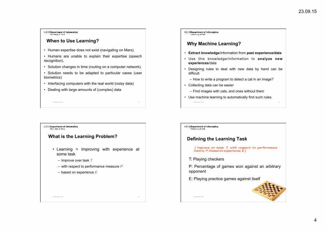
Classification •  Two main phases:

–  Training: Learn the classification model from labeled data.

–  Prediction: Use the pre-built model to classify new instances.

•  Classification can be binary (two classes), or over a larger number of classes (multi-class). –  In binary classification we often refer to one class as

“positive”, and the other as “negative”

•  Binary classifier creates a boundaries in the input space between areas assigned to each class 23 September 2015 30

Classification using Decision Boundaries

A set of straight line decision boundaries for a classification problem.

An alternative set of decision boundaries that separate the plusses from lightening strikes better, but it requires a line that isn’t straight.

Regression •  Regression analysis is used to predict the value of one

variable (the dependent variable) on the basis of other variables (the independent variables).

•  Learn a continuous function.


•  Given, the following data, can we find the value of the output when x = 0.44?

•  Goal is to predict for input x an output f(x) that is close to the true y.

•  It is generally a problem of function approximation, or interpolation, working out the value between values that we know.

Which line has the best “fit” to the data?

•  Top left: A few data points from a sample problem. Bottom left: Two possible ways to predict the values between the known data points: connecting the points with straight lines, or using a cubic approximation (which in this case misses all of the points). Top and bottom right: Two more complex approximators that passes through the points, although the lower one is rather better than the top.


23.09.15

9

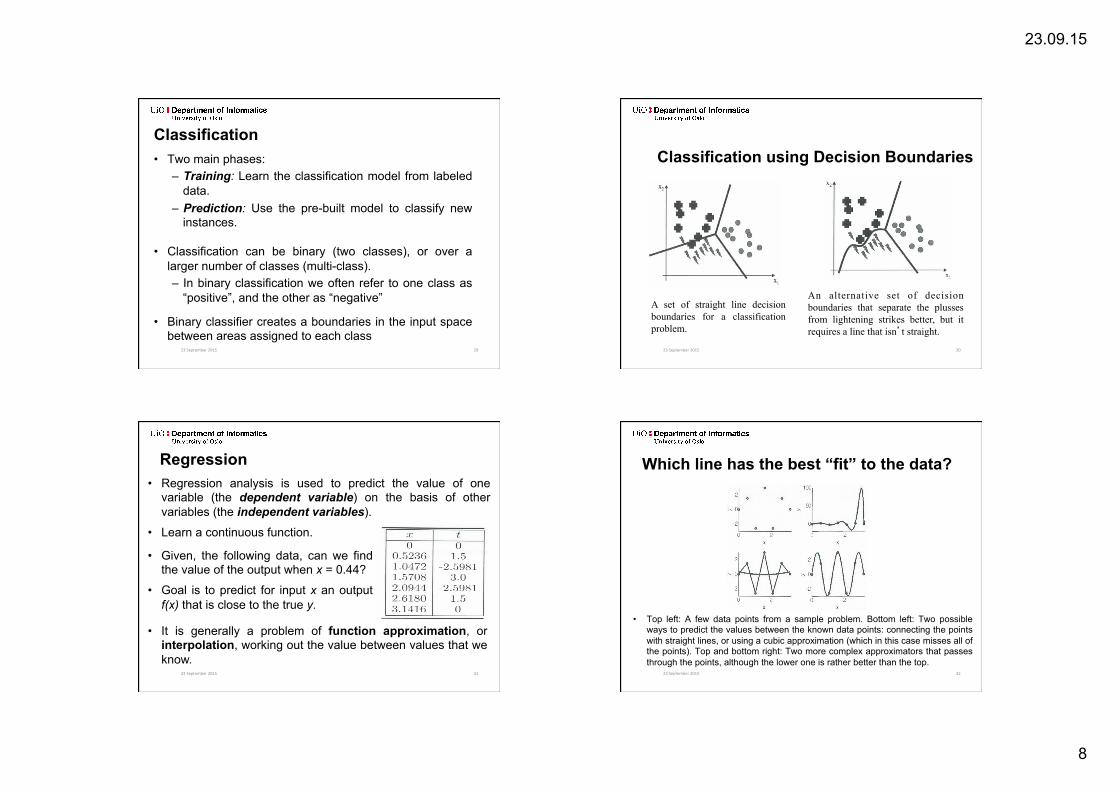
The Machine Learning Process

1.  Data Collection and Preparation 2.  Feature Selection and Extraction 3.  Algorithm Choice 4.  Parameters and Model Selection 5.  Training 6.  Evaluation

33

Neural Networks •  We are born with about 100 billion neurons •  A neuron may connect to as many as 10,000

other neurons

•  Much parallel computation


Neural Networks •  Neuron: many-inputs / one-output unit. •  Neurons are connected by synapses •  Signals “move” via electrochemical signals on a

synapse

•  The synapses release a chemical transmitter, enough of which can cause a neuron threshold to be reached, causing the neuron to “fire”

•  Synapses can be inhibitory or excitatory •  Learning: Modification in the synapses


Hebb’s Rule


•  Strength of a synaptic connection is proportional to the correlation of two connected neurons.

•  If two neurons consistently fire simultaneously, synaptic connection is increased (if firing at different time, strength is reduced).

•  “Cells that fire together, wire together.”

23.09.15

10

McCulloch and Pitts Neurons

•  McCulloch & Pitts (1943) are generally recognised as the designers of the first artificial neural network.

•  Many of their ideas still used today (e.g. many simple units combine to give increased computational power and the idea of a threshold).



•  Greatly simplified biological neurons. •  Sum the weighted inputs

•  If total is greater than some threshold, neuron “fires” •  Otherwise does not

38

x2

xm

w1

w2

wm

o h

x1

θ


•  The weight wj can be positive or negative •  Inhibitory or exitatory.

•  Use only a linear sum of inputs. •  Synchronous processing. •  No resting state following excitation. •  Scalar output instead of a pulse (spike train). 39

for some threshold θ

Biologically Inspired •  Electro-chemical signals. •  Threshold output firing.


Axon

Terminal Branches of AxonDendrites

23.09.15

11

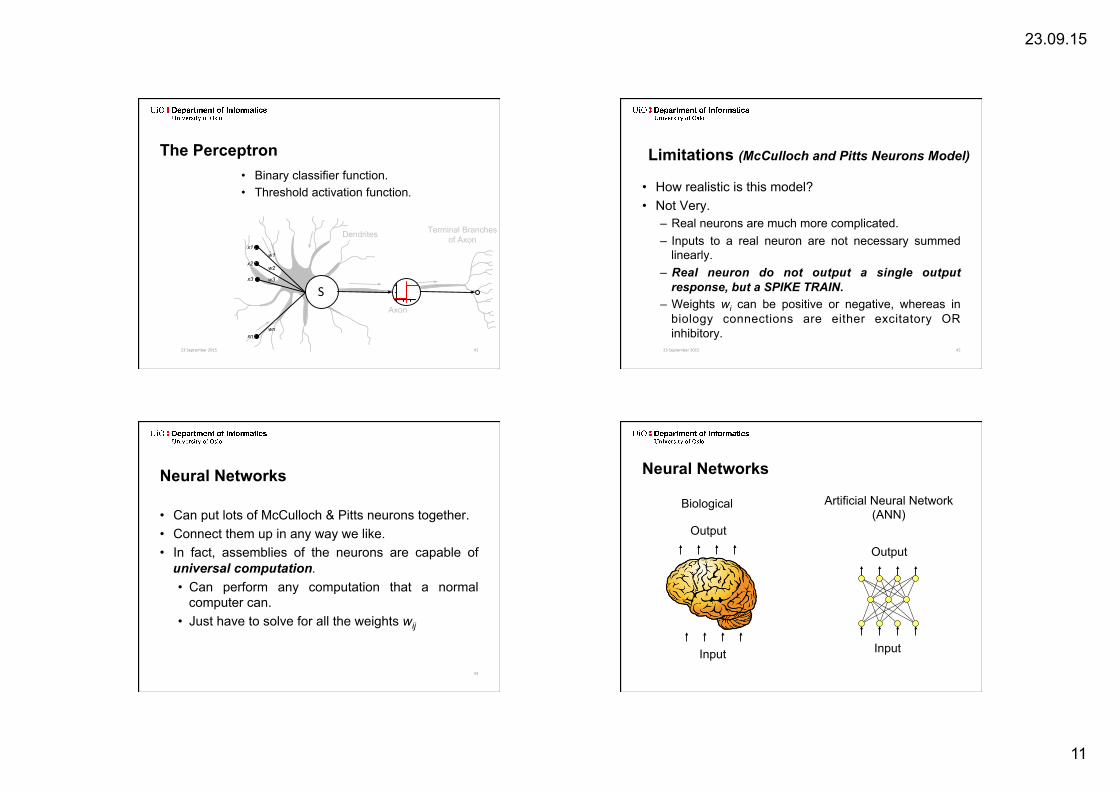
The Perceptron •  Binary classifier function. •  Threshold activation function.


Axon

Terminal Branches of AxonDendrites

S

x1

x2w1

w2

wnxn

x3 w3

Limitations (McCulloch and Pitts Neurons Model)

•  How realistic is this model? •  Not Very.

–  Real neurons are much more complicated. –  Inputs to a real neuron are not necessary summed

linearly. –  Real neuron do not output a single output

response, but a SPIKE TRAIN. –  Weights wi can be positive or negative, whereas in

biology connections are either excitatory OR inhibitory.


Neural Networks

•  Can put lots of McCulloch & Pitts neurons together. •  Connect them up in any way we like. •  In fact, assemblies of the neurons are capable of

universal computation. •  Can perform any computation that a normal

computer can. •  Just have to solve for all the weights wij

43

Neural Networks

Input

Output

Biological Artificial Neural Network (ANN)

Input

Output

23.09.15

12

The Perceptron Network

45

Inputs Outputs

Training Neurons

•  Adapting the weights is learning •  How does the network know it is right? •  How do we adapt the weights to make the network

right more often?

•  Training set with target outputs (supervised learning).

•  Learning rule.

46

A Simple Perceptron

•  One unit (the loneliest network)

•  Change the weights by an amount proportional t o t h e d i f f e r e n c e between the desired output and the actual output.


wij ← wij + Δ wij

Updating the Weights

•  Aim: minimize the error at the output •  If E = t-y, want E to be 0 •  Use:

48

Learning rate

Error

Input

Desired output Actual output

23.09.15

13

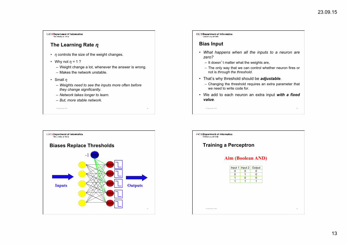
The Learning Rate ɳ

•  ɳ controls the size of the weight changes.

•  Why not ɳ = 1 ? –  Weight change a lot, whenever the answer is wrong. –  Makes the network unstable.

•  Small ɳ –  Weights need to see the inputs more often before

they change significantly. –  Network takes longer to learn. –  But, more stable network.


Bias Input •  What happens when all the inputs to a neuron are

zero? –  It doesn’t matter what the weights are, –  The only way that we can control whether neuron fires or

not is through the threshold.

•  That’s why threshold should be adjustable. –  Changing the threshold requires an extra parameter that

we need to write code for.

•  We add to each neuron an extra input with a fixed value.


Biases Replace Thresholds

51

Inputs Outputs

-1

Training a Perceptron


Input 1 Input 2 Output 0 0 0 0 1 0 1 0 0 1 1 1

Aim (Boolean AND)

23.09.15

14



t = 0.0

y

x

-1 W0 = 0.3

W2 = -0.4

W1 = 0.5

I1 I2 I3 Summation Output -1 0 0 (-1*0.3) + (0*0.5) + (0*-0.4) = -0.3 0 -1 0 1 (-1*0.3) + (0*0.5) + (1*-0.4) = -0.7 0 -1 1 0 (-1*0.3) + (1*0.5) + (0*-0.4) = 0.2 1 -1 1 1 (-1*0.3) + (1*0.5) + (1*-0.4) = -0.2 0



t = 0.0

y

x

-1 W0 = 0.3

W2 = -0.4

W1 = 0.5

I1 I2 I3 Summation Output -1 1 0 (-1*0.55) + (1*0.25) + (0*-0.4) = -0.3 1 0

W0 = 0.3 + 0.25 * (0-1) * -1 = 0.55 W1 = 0.5 + 0.25 * (0-1) * 1 = 0.25 W2 = -0.4 + 0.25 * (0-1) * 0 = -0.4

W0 = 0.55

W1 = 0.25 W2 = -0.4

η = 0.25

Linear Separability

55

w

More Than One Neuron

•  The weights for each neuron separately describe a straight line. 23 September 2015 56

23.09.15

15

Perceptron Limitations

•  A single layer perceptron can only learn linearly separable problems. –  Boolean AND function is linearly separable, whereas

Boolean XOR function (and the parity problem in general) is not.


Linear Separability


Boolean AND Boolean XOR

What Can Perceptrons Represent?


0,0

0,1

1,0

1,1

0,0

0,1

1,0

1,1

AND XOR

•  Only linearly separable functions can be represented by a perceptron

60

Linear Separability The Exclusive Or (XOR) function A B Out 0 0 0 0 1 1 1 0 1 1 1 0

Limitations of the Perceptron

23.09.15

16

61

Limitations of the Perceptron

? W1 > 0 W2 > 0 W1 + W2 < 0


•  Multi-layer perceptron can solve this problem

•  More than one layer of perceptrons (with a hardlimiting activation function) can learn any Boolean function

•  A learning algorithm for multi-layer perceptrons was not developed until much later •  backpropagation algorithm (replacing the hardlimiter with a

sigmoid activation function)


Perceptron Limitations •  XOR problem: What if we use more layers of

neurons in a perceptron? •  Each neuron implementing one decision boundary and the

next layer combining the two?

23 September 2015 63 64


A decision boundary (the shaded plane) solving the XOR problem in 3D with the crosses below the surface and the circles above it.

23.09.15

17



Left: Non-separable 2D dataset. Right: The same dataset with third coordinate x1 x x2, which makes it separable.

Decision Boundaries

66

x1

x2

Decision Boundaries

67

x1

x2

The Multi-Layer Perceptron

68

Input Layer

Hidden Layer Output Layer

-1 -1

23.09.15

18

MLP Decision Boundary – Nonlinear Problems, Solved!


In contrast to perceptrons, multilayer networks can learn not only multiple decision boundaries, but the boundaries may be nonlinear.

Input nodes Internal nodes Output nodes

X2

X1

And Finally….

“If the brain were so simple that we could understand it then we’d be so simple that we couldn’t”


-- Lyall Watson

Documents

Jim Tørresen - uio.no · Jim Tørresen This Lecture 1. ... think, learn, understand language, ++ ... Minsky and Papert prove limitations of Perceptron 1970s