Embed Size (px)
Citation preview
§ This work is part of the research carried out at Oslo Fiscal Studies, which is supported by the Research Council of Norway.
The authors thank Odd Erik Nygård for providing the consumption data. We have benefited from comments by Spencer Bastani and seminar participants of the ETI workshop in Mannheim, August 2015, to an earlier version of the paper. * Oslo Fiscal Studies (Department of Economics, University of Oslo), email: [email protected] **Statistics Norway, Oslo Fiscal Studies (Department of Economics, University of Oslo), and CESifo (Munich), email: [email protected]
ON THE TAX RESPONSE ANATOMY OF THE
SELF-EMPLOYED§
by Kristoffer Berg* and Thor O. Thoresen**
Abstract
The elasticity of taxable income (ETI) encompasses responses along several margins in general, but it
is commonly acknowledged that the overall ETI of the self-employed in particular reflects a multitude
of behavioral reactions to tax changes. Besides that policy design discussions benefit from addressing
information about the composition of the self-employment ETI, further investigation of the various
forms of responses of and their magnitudes are also important for obtaining non-biased ETI
estimates. This paper discusses the tax induced behavioral anatomy of self-employed in Norway by
exploiting evidence from a broad range of data sources, using reductions in marginal tax rates due to
the tax reform of 2006 for identification. Separate evidence on how the tax changes affected working
hours, organizational shifts, shifting between different tax bases and income reporting are
presented. We find a moderate overall tax effect on income for the self-employed, predominantly
explained by (real) behavioral effects in working hours.
2
1. Introduction After Feldstein (1995) it has become widespread to obtain estimates of tax induced responses in
income by analyzing panel data over a tax reform period, exploiting the variation in changes in
marginal tax rates across individuals. The focus has mainly been on the elasticity of taxable income
(ETI), which is a crude overall measure of the responses to tax changes. As the ETI in principle
captures all tax-induced responses and as it can be derived by standard econometric tools, the ETI
measurement has become a popular empirical strategy for summarizing the efficiency costs of
taxation, see Saez, Slemrod and Giertz (2012).
Even though the ETI estimate for any taxpayer may reflect a variety of tax behavioral effects,
as emphasised by Feldstein (1995), there are some important response dimensions that are known
to be particularly relevant for the self-employed. For example, the self-employed have wider scope
for underreporting of income and they may react to tax changes by choosing to run their businesses
under other organizational forms. Both from an econometric identification perspective and with
respect to the understanding of economic implications of estimates, it becomes essential to obtain
more information about components of the ETI for the self-employed. For example, are the ETIs for
the self-employed large because they comprise a variety of responses, and do overall effects
therefore predominantly reflect various types of income shifting and less real responses, such as
changes in investments and labor supply? Welfare implications of reforms depend on the relative
importance of the different adjustment channels (Slemrod, 1996; Chetty, 2009).
Whereas estimates of the ETI for wage earners have been obtained for a wide selection of
countries,1 there are much fewer studies using the ETI framework for obtaining estimates of tax
responsiveness for the self-employed; exceptions include Wu (2005), Blow and Preston (2002), Heim
(2010), Kleven and Schultz (2014).2 These previous discussions of the ETI for the self-employed have
typically provided little information about the behavioral anatomy of the tax responses, and rather
relegated interpretational complications to verbal reservations in the discussions of estimates.3 The
present paper uses the reductions in the marginal tax rates of the Norwegian tax reform of 2006 to
explore different response dimensions for the self-employed. This enriches the understanding of the
driving forces behind the overall response in the ETI due to the reform and, in particular, is important
for obtaining non-biased estimates of the overall (total) ETI.
1 Estimates for the U.S. can be found in Auten and Carroll (1999) and Gruber and Saez (2002), whereas Aarbu and Thoresen (2001), Blomquist and Selin (2012), and Kleven and Schultz (2014) deliver ETI estimates for Norway, Sweden and Denmark, respectively. 2 To be precise, Wu (2005) estimates the responsiveness of “privately held businesses”. Note that also le Maire and Schjerning (2013) and Bastani and Selin (2014) estimate taxable income elasticities for the self-employed, but both use bunching techniques for identification. 3 Heim (2010) presents results where the data sample has been adjusted to control for shifting across tax bases and across years.

3
Before explaining the different components of our empirical approach in further detail, let us
briefly restate the standard method of obtaining ETI estimates. The ETI provides an intensive margin
response, which is identified by addressing information on taxable income over a period where there
is variation in the net-of-tax rate (1 minus the marginal tax rate), generated by a tax reform.
Following Feldstein (1995) the great majority of empirical studies of the ETI have used panel data in
the identification,4 where first differenced income (in log) for each individual in the panel is regressed
against an expression for the change in tax (in log). To allow the new tax prices to be absorbed by the
agents, it has become standard to use three-year span in data from pre-reform to post-reform.
Following Auten and Carroll (1999), Moffitt and Wilhelm (2000), and Gruber and Saez (2002), most
studies use an instrument for the change based on statutory tax changes, obtained by letting the tax
law at time t and (say) time t+3 mechanically be applied to the same pre-reform incomes, and
estimate the differenced equation with 2SLS.
In the present study we use the changes according to the Norwegian tax reform of 2006 to
obtain ETI estimates for the Norwegian self-employed. Given the intensive margin perspective,
conditioning on being self-employed in both periods (t and time t+3) accords with the standard
empirical framework. This is an innocuous sample selection condition as long as the tax changes do
not induce taxpayers to move out of the personal income tax base. However, several studies, as
Slemrod (1995), Gordon and Slemrod (2000), Goolsbee (2004), Thoresen and Alstadsæter (2010), and
Edmark and Gordon (2013) advice against ignoring organizational shifts when discussing tax
responses. This aspect is specifically critical in the present context, as under the tax schedule prior to
the tax reform used to obtain estimates here, Thoresen and Alstadsæter (2010) found evidence of
tax motivated organizational shifts (increasing in the level of income). Taxpayers moved out of the
so-called split model for the self-employed, and took advantage of the lower taxation of capital
income (dividends). As the Norwegian tax reform of 2006 involved tax changes meant to abolish
these incentives (Sørensen, 2005),5 there are reasons to take a closer look at this responsive margin.
If the tax reform has stopped these movements, it means that more people remain in our self-
employment data sample after the reform, compared to the counterfactual situation, without a
reform. Then the business owners most likely have self-selected to remain in the sample of self-
employed, which means that they represent a non-random addition to our experimental group. For
example, many of them are expected to have high income, as seen in Thoresen and Alstadsæter
(2010). If not precautionary measures are taken, we are in danger of erroneously attributing their
4 However, Lindsey (1987) used repeated cross-sections. See also Goolsbee (1999). 5 In addition to the reduction in marginal tax rates, this is achieved through an individual tax on dividend incomes and capital gains above a rate-of-return allowance, that is, on profits above a risk free rate of return, by 48.2 percent at the maximum in 2006.
4
behavior to the reductions in marginal tax rates, potentially generating biased results in the
estimation of the overall ETI.
We are able to investigate the effects of patterns of organizational shifts because of the
richness in the data we have had available for this study. The main data source is the yearly Income
statistics for families and persons, which is based on information from administrative registers (as
the Register of tax returns), covers the whole population, and can be turned into a panel data set
through personal id numbers with a large set of control variables. Observations for the period from
2001 to 2010 from this data source are used in the present analysis. Further, we need to combine
these income data with three other data sources in order to explore the extent of organizational
shifts: information from the Business and enterprise register (Virksomhet og foretaksregisteret), the
Shareholder register (Aksjonærregisteret) and the End of the year certificate register (Lønns- og
trekkoppgaveregisteret). By combining information from these three data sources and the income
data, we find those who have moved out of self-employment to be a shareholder in the same firm as
he/her is employed. Any difference in these movements from the pre-reform period to the post-
reform period is taken as corroborative evidence of a possible measurement problem in the ETI
estimation.
Next, we discuss effects of the increase in the net-of-tax rate both with respect to changes in
income and in working hours, assuming that the latter definition of the dependent variable captures
an important “real effect” component of the overall ETI. In the estimation of the working hours
component we use information from the Labour force survey, which is a repeated cross-section
sample survey. Thus, a standard difference-in-differences empirical strategy is used to obtain
estimates of the elasticity with respect to working hours, analogous to the elasticity obtained for
income (ETI).
Further, we examine another particularly important response margin for the self-employed,
namely tax evasion, to see if there is a tax evasion component of the ETI. In fact, the so-called
expenditure approach for identification of tax evasion (Pissarides and Weber, 1989) is based on a
comparison of wage earners and the self-employed, where only the latter group is assumed to
evade. Here we use information from the Survey of consumer expenditure to estimate expenditure
functions (i.e., Engel curves for food) for wage earners and the self-employed, which are then used to
calculate the amount by which reported income must be scaled up by in order to obtain true income
levels for tax evaders. As we have data for pre-reform and the post-reform periods, any differences
in the estimated tax evasion between the two periods can be attributed to the increase in the net-of-
tax rate after the 2006-reform, reflected in the overall ETI estimate. It should be noted that neither
5
the theoretical contribution nor the empirical evidence point to clear predictions on the relationship
between marginal tax rates and tax evasion (Slemrod, 2007).6
As the standard empirical approach for obtaining estimates of the ETI involves using the
changes according to one or several tax reforms, another complication comes from wrongly
attributing effects of other simultaneously implemented schedule changes to the net-of-tax rate
adjustments. The reform used for identification in the present paper clearly illustrates this
complication, as the tax reform of 2006 has a relatively far-reaching change in the capital as its other
main feature, in addition to the reduction in the marginal tax rate. Thus, we shall also probe deeper
into this response dimension.
The paper is organized as follows. The Norwegian tax system and the changes in it according
to the 2006-reform is described in Section 2, whereas Section 3 describes how we can derive
information about responses from some of the most important margins, in addition to the overall ETI
estimate, given the tax changes of the reform. The empirical evidence is presented in Section 4, and
Section 5 concludes the paper.
2. The Norwegian dual income tax and the reform of 2006 The tax reform of 1992 introduced a version of the dual income tax in Norway, a combination of a
low proportional tax rate on capital income and progressive tax rates on labor income. This system
proliferated throughout the Nordic countries in the early 1990s, and the Norwegian version had a flat
28 percent tax rate levied on corporate income, capital and labor income coupled with a social
security contribution and a progressive surtax applicable to labor income. Double taxation of
dividends was abolished, as taxpayers receiving dividends were given full credit for taxes paid at the
corporate level, and the capital gain tax system exempted gains attributable to retained earnings
taxed at the corporate level. These separate schedules for capital and labor income created obvious
incentives for taxpayers to recharacterize labor income as capital income. To limit such tax
avoidance, the 1992 reform introduced the ‘‘split model’’ for the self-employed, partnerships and
closely held firms; the latter defined as businesses in which more than two-thirds of the shares were
owned by the active owner(s). Rules were established for dividing business income into capital and
labor income by imputing a return to business assets and attributing the residual income to labor.
Labor income was subject to a social security contribution and two-tier surtax, and the top marginal
tax rates for wage earners and owners of small businesses (the self-employed, partners and owners
6 For example, the early contributions of Allingham and Sandmo (1972) and Yitzhaki (1974) point to ambiguous effects. In fact, according to the latter study, if the absolute risk aversion is increasing in income, and the penalty for cheating is proportional to the tax evaded, evasion is decreasing in the tax rate.
6
of closely held firms) were 48.8 percent7 and 51.7 percent in 1992. Between 1992 and 2004, both the
threshold for the second tier of the surtax and marginal rates increased, resulting in the statutory tax
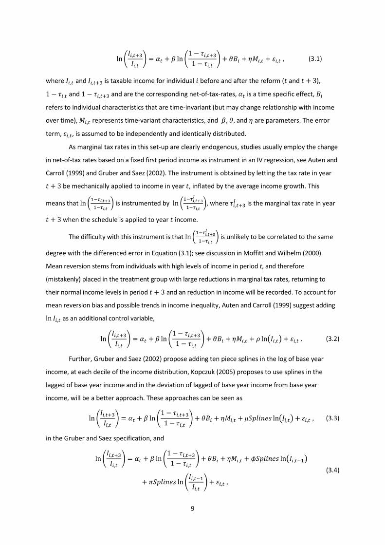
rates as shown for 2004 (the last year before the reform) in Figure 1, with 55.3 percent at the
maximum.
Under the split model, an imputed return to the capital invested in the firm is calculated by
multiplying the value of the capital assets by a fixed rate of return on capital. This imputed return to
capital is taxed by the corporate tax rate, which also equals the capital income tax rate at the
individual level, fixed at 28 percent in the time period under consideration here. Business profit net
of imputed return to capital is the imputed return to labor, which is taxed as labor income, so-called
personal income, independently of whether the income is retained in the firm or transferred to the
owner.
The main idea was that taxation of “labor income” would follow a similar schedule,
independent of whether the income came from regular wage payments or was obtained by the split
model. However, the 1990s saw increasing pressure on the dual income tax system, resulting in
numerous “patches.”8 Most importantly, given the present context, a distinction between liberal
professions (lawyers, dentists, doctors and other independent contractors delivering services to the
public) and other professions was introduced in terms of ceilings were the labor income part is taxed
by the capital income tax rate (28 percent). It appears that it was believed that the split-model was
more appropriate for non-liberal professions. At least, the special ceilings for the liberal occupations
were abolished in 1998, whereas the ceilings for other professions were kept until the split model
was eliminated in 2004. In the description of schedules before and after the reform, in Figure 1, the
lower ceilings for the self-employed belonging to non-liberal professions are seen in the lower panel:
incomes in the interval from approximately 1 million Norwegian kroner (NOK)9 to approximately 4,7
million NOK and from approximately 8,3 million NOK and onward in the schedule for 2004 are not in
the surtax income base, but only taxed by the 28 percent.
7 Excluding the employers’ social security contribution. 8 Christiansen (2004) sees this as resulting from political games motivated in part by the concerns of politicians of various colors with special interest groups. 9 The intervals were defined through the so-called “basic amount” (G) in the social insurance system. In 2004 the low-rate intervals are between 16 G and 75 G and from 134 G and onward. The thresholds in Figure 1 are measured in terms of the 2006-value for G, equal to 62,161 NOK. Use exchange rates of one US dollar for 6.42 NOK and one Euro for 8.05 NOK to convert to other currencies.
7
Figure 1. Marginal tax rates for the self-employed in 2004 and 2006. Income < 1 mill. NOK in upper panel, income in interval [0.8,10] mill. NOK in lower panel
*1 mill NOK ≈ $ 156,000, ≈ € 124,000, in 2006.
The reform of 2006 emerged as an attempt to create a system that would prevent taxpayers
from transforming labor income into capital income to benefit from the lower flat rate applied to the
latter; see Sørensen (2005) for the wider background to the reform and steps taken to adjust the
0
10
20
30
40
50
60
150 000 250 000 350 000 450 000 550 000 650 000 750 000 850 000 950 000
Marginal tax
Wage income
2004
2006
0
10
20
30
40
50
60
800 000 1 800 000 2 800 000 3 800 000 4 800 000 5 800 000 6 800 000 7 800 000 8 800 000 9 800 000
Marginal tax
Wage income
2004, non-liberalprofessions
2004, liberalprofession
2006
8
dual income tax. Individual dividend incomes and capital gains above a rate-of-return allowance, that
is, on profits above a risk free rate of return, were taxed at 48.2 percent at the maximum in 2006.10
Moreover, and particularly important in the present context, top marginal tax rates on wage
income were cut to narrow the differences between the marginal tax rates on capital income and
labor income, see Figure 1. However, as already denoted, some groups of the self-employed
experienced a decrease in the net-of-tax rate after the reform (see the lower panel), which will be
accounted for in the empirical analysis. After the revision of the dual income tax in 2006, the owners
of sole proprietorships are taxed under the self-employment model (foretaksmodellen), which shares
important similarities with the split-model. According to the new rules, business income from a sole
proprietorship activity in excess of the risk-free return allowance, calculated on the invested capital,
is taxed as imputed personal income and is subject to surtax and social security contribution.11
Of course, one may ask if the tax reform is large enough to overcome adjustments costs and
induce people to find a new optimum, as discussed by Chetty (2012). However, we believe that there
are less adjustments costs involved in several of the response margins for the self-employed,
compared to what is the case for wage earners.
3. The response margins and identification strategies
3.1 Estimation of the overall ETI
In the following we shall present the empirical strategies to obtain information about different
response margins. First, we shall present how the overall ETI is identified, following well-known
empirical specifications seen in the literature after Feldstein (1995), see, for example, Auten and
Carroll (1999), Moffitt and Wilhelm (2000), Gruber and Saez (2002), and Kopczuk (2005).
As already mentioned in the Introduction, income panel data (Statistics Norway, 2005)
covering a period of net-of-tax rate variation across individuals and across time have been the main
data source for the identification of responses in the ETI literature.12 As one has settled down on
measuring three-year differences in income, the estimated equation can be seen as
10 The figure for the marginal tax rate on dividends in 2006 is derived as follows. Capital income is taxed at a 28 percent rate at the corporate level, and the remaining 72 percent is transferred to the individual and taxed at 28 percent (above the rate of return allowance), resulting in a combined rate of 20.16 percent (0.72×0.28), which is then added to the corporate level rate. Now, in 2015, the corporate is reduced to 27, which alters the calculation correspondingly. 11 The basis for calculation of risk-free rate is the arithmetic average observed on the treasury bills with 3 months maturity, as published by Norges Bank every year. In 2014 it was 1.24 percent. 12 Note that there is another acronym too: Goolsbee (1999) refers to studies in this field as belonging to the “new tax responsiveness literature” (NTR).
9
ln (𝐼𝑖,𝑡+3
𝐼𝑖,𝑡) = 𝛼𝑡 + 𝛽 ln (
1 − 𝜏𝑖,𝑡+3
1 − 𝜏𝑖,𝑡) + 𝜃𝐵𝑖 + 𝜂𝑀𝑖,𝑡 + 𝜀𝑖,𝑡 , (3.1)
where 𝐼𝑖,𝑡 and 𝐼𝑖,𝑡+3 is taxable income for individual 𝑖 before and after the reform (𝑡 and 𝑡 + 3),
1 − 𝜏𝑖,𝑡 and 1 − 𝜏𝑖,𝑡+3 and are the corresponding net-of-tax-rates, 𝛼𝑡 is a time specific effect, 𝐵𝑖
refers to individual characteristics that are time-invariant (but may change relationship with income
over time), 𝑀𝑖,𝑡 represents time-variant characteristics, and 𝛽, 𝜃, and 𝜂 are parameters. The error
term, 𝜀𝑖,𝑡, is assumed to be independently and identically distributed.
As marginal tax rates in this set-up are clearly endogenous, studies usually employ the change
in net-of-tax rates based on a fixed first period income as instrument in an IV regression, see Auten and
Carroll (1999) and Gruber and Saez (2002). The instrument is obtained by letting the tax rate in year
𝑡 + 3 be mechanically applied to income in year 𝑡, inflated by the average income growth. This
means that ln (1−𝜏𝑖,𝑡+31−𝜏𝑖,𝑡
) is instrumented by ln (1−𝜏𝑖,𝑡+3𝐼
1−𝜏𝑖,𝑡), where 𝜏𝑖,𝑡+3
𝐼 is the marginal tax rate in year
𝑡 + 3 when the schedule is applied to year 𝑡 income.
The difficulty with this instrument is that ln (1−𝜏𝑖,𝑡+3𝐼
1−𝜏𝑖,𝑡) is unlikely to be correlated to the same
degree with the differenced error in Equation (3.1); see discussion in Moffitt and Wilhelm (2000).
Mean reversion stems from individuals with high levels of income in period t, and therefore
(mistakenly) placed in the treatment group with large reductions in marginal tax rates, returning to
their normal income levels in period 𝑡 + 3 and an reduction in income will be recorded. To account for
mean reversion bias and possible trends in income inequality, Auten and Carroll (1999) suggest adding
ln 𝐼𝑖,𝑡 as an additional control variable,
ln (𝐼𝑖,𝑡+3
𝐼𝑖,𝑡) = 𝛼𝑡 + 𝛽 ln (
1 − 𝜏𝑖,𝑡+3
1 − 𝜏𝑖,𝑡) + 𝜃𝐵𝑖 + 𝜂𝑀𝑖,𝑡 + 𝜌 ln(𝐼𝑖,𝑡) + 𝜀𝑖,𝑡 . (3.2)
Further, Gruber and Saez (2002) propose adding ten piece splines in the log of base year
income, at each decile of the income distribution, Kopczuk (2005) proposes to use splines in the
lagged of base year income and in the deviation of lagged of base year income from base year
income, will be a better approach. These approaches can be seen as
ln (𝐼𝑖,𝑡+3
𝐼𝑖,𝑡) = 𝛼𝑡 + 𝛽 ln (
1 − 𝜏𝑖,𝑡+3
1 − 𝜏𝑖,𝑡) + 𝜃𝐵𝑖 + 𝜂𝑀𝑖,𝑡 + 𝜇𝑆𝑝𝑙𝑖𝑛𝑒𝑠 ln(𝐼𝑖,𝑡) + 𝜀𝑖,𝑡 , (3.3)
in the Gruber and Saez specification, and
ln (𝐼𝑖,𝑡+3
𝐼𝑖,𝑡) = 𝛼𝑡 + 𝛽 ln (
1 − 𝜏𝑖,𝑡+3
1 − 𝜏𝑖,𝑡) + 𝜃𝐵𝑖 + 𝜂𝑀𝑖,𝑡 + 𝜙𝑆𝑝𝑙𝑖𝑛𝑒𝑠 ln(𝐼𝑖,𝑡−1)
+ 𝜋𝑆𝑝𝑙𝑖𝑛𝑒𝑠 ln (𝐼𝑖,𝑡−1
𝐼𝑖,𝑡) + 𝜀𝑖,𝑡 ,
(3.4)
10
in the Kopczuk specification.
In Section 4 we shall present results for estimations of Equations (3.2), (3.3) and (3.4), using
2SLS and the net-of-tax rate instrument is as specified above, and controlling for a number of other
characteristics (in 𝐵𝑖 and 𝑀𝑖,𝑡).
3.2 Response in working hours
A key question is how much of the response in the ETI comes from real labor supply adjustments to
the reform. One way to address this is to use the same regressors as for income to estimate an
equation with the difference in working hours as the regressand. Fewer available data sets with a
panel dimension on working hours most likely explain why we see fewer studies with changes in
working hours as the dependent variable.13 However, as emphasized by Saez, Slemrod and Giertz
(2012), cross-sectional data can straightforwardly be used to obtain ETI estimates, and here we shall
use several cross-sections of the Labor force survey (2001–2010) (Statistics Norway, 2003) to obtain a
similar response estimate for working hours for the self-employed.14
Given that we have access to information about working hours through cross sectional data,
a possible identification strategy is to divide observations into “experimental group” and “control
group”, and apply the standard difference-in-differences estimator for identification.15 The
framework can then be seen as
ℎ𝑖,𝑡 = 𝛼 + 𝛾𝐷𝑖 + 𝜆𝑄𝑡 + 𝛿𝐷𝑖𝑄𝑡 + 𝜃𝐵𝑖 + 𝜂𝑀𝑖,𝑡 + 𝜖𝑖,𝑡 , (3.5)
where ℎ𝑖,𝑡 is working hours, 𝛼 is a constant, 𝐷𝑖 is a dummy variable for being in the experimental
group, 𝑄𝑡 is a time dummy variable for the post-reform period, and as before, 𝐵𝑖 and 𝑀𝑖,𝑡 refer to
time-invariant and time-variant individual characteristics, respectively, and 𝜀𝑖,𝑡 is the error term. 𝛾, 𝜆,
and 𝛿 are paramters, and 𝛿 measures the effect of the reform on working hours.
To allocate observations into experimental and control groups we use individual calculations
of net-of-tax rates, similarly to the net-of-tax rate instrument used in Section 3.1. As we have
personal identification numbers, we are able to add information based on data from the Income
statistics for person and families (net-of-tax rates) to the samples used to obtain estimates for
working hours.
3.3 Contribution from tax evasion
Next, as it is well established that the self-employed have more scope for tax evasion than wage
earners, there are reason to explore, when discussing the self-employment ETI, how much of the 13 Note also that Feldstein (1995; 1999) convincingly argues that the ETI summarizes the welfare cost of income taxation. See also Chetty (2009) on this. 14 Thoresen and Vattø (2015) use Norwegian register data on working hours for wage earners, but no such data are available for the self-employed. 15 Angrist and Pischke (2009) provide several examples of use of this technique.
11
response in the ETI which can be attributed to tax evasion. However, even though the self-employed
are known to underreport income, how they react to tax changes appears to be less obvious. The
theoretical literature, as Allingham and Sandmo (1972) and Yitzhaki (1974), offers no clear answers,16
and the empirical findings are mixed. Some of the early studies, as Clotfelter (1983), find increased
tax evasion for higher marginal tax rates, whereas, for example, Kleven et al. (2011) find a negative
relationship.
Nevertheless, we look for altered tax evasion behavior after the reform by addressing tax
response estimates derived by the so-called expenditure approach (Pissarides and Weber, 1989). The
method relies on one group reporting income correctly and another not, but both groups reporting
food expenditures17 truthfully. Thus, this part of the study uses consumption data from the Survey of
consumer expenditure (Holmøy and Lillegård, 2014). When also assuming that the two groups share
the same preferences for food, given a set of observable characteristics, estimates on the degree of
underreporting among evading households are obtained by exploiting observations on income and
food expenditures for both types of households. More precisely, a common point of departure is the
following log-linear Engel function,
ln 𝐶ℎ = 𝜓𝑍ℎ + 𝜉 ln 𝑌ℎ∗, (3.6)
where ln 𝐶ℎ is the natural log of food expenditure for household, h, 𝑍ℎ is a set of observable
household characteristics, and ln 𝑌ℎ∗ is the natural log of the “true” disposable income.18 The
coefficient 𝜉 is the Engel elasticity for food consumption with respect to true disposable income,
assumed identical for all households. A standard assumption is that underreporting takes place at a
constant fractions such that, 𝑌ℎ∗ = 𝑘𝑌ℎ where 𝑌ℎ is the reported income and 1k ! if underreporting
takes place. Taking the natural log of this expression and substituting into Equation (3.6) leads to
ln 𝐶ℎ = 𝜓𝑍ℎ + 𝜉(ln 𝑌ℎ + ln 𝑘). Thus, the Engel function coincides with (3.6) for those declaring all
their income (𝑘 = 1), but gets a shift for those underreporting (𝑘 > 1). The Engel elasticity with
respect to reported income stays the same as the Engel elasticity with respect to the total, true,
income. The studies based on the expenditure approach predominantly uses the self-employed as
candidates for underreporting,19 and the following reduced form specification is often used,
ln 𝐶ℎ = 𝜓𝑍ℎ + 𝜇 ln 𝑌ℎ + 𝜅𝑆𝐸ℎ + 𝑢ℎ, (3.7)
16 In the model of Allingham and Sandmo (1972) a tax increase has two contradicting effects: the return to cheating goes up, but at the same time it lowers (full compliance) post-tax income, which most likely make people more risk averse. In the model of Yitzhaki (1974), in contrast to Allingham and Sandmo, the penalty is proportional to the tax evaded, which leads to more evasion for a tax raise. 17 Feldman and Slemrod (2007) is an example of a study using another type of consumption for identification, as they relate consumption of charity to income. 18 Thus, reflecting that the household is the economic unit in the consumption data. 19 The income and deductions of wage earners are primarily third-party reported in Norway, which is believed to limit the scope for tax evasion.
12
where hSE is a self-employment dummy. A positive 𝜅 suggests that these households underreport
income, and given that we would like to obtain an estimate for the number which can be used to
multiply self-employment income with in order to obtain “true income”, we have 𝑘 = exp (𝜅𝜇
) . 20
Several studies report estimates of 𝑘, for example give Johansson (2005) and Engström and
Holmlund (2009) estimates for Finland and Sweden, respectively. In the present study we exploit this
technique to investigate to what extent changes in tax evasion contribute to the estimate of the
overall ETI.
3.4 Controlling for organizational shifts
As seen in Thoresen and Alstadsæter (2010), even though the taxation of the self-employed includes
intervals with lower taxes (see Figure 1), the dual income tax schedule prior to 2006 gave incentives
for the self-employed to incorporate and take advantage of the receiving payments in terms of low-
taxed dividends instead of wage earnings. Therefore, if the tax reform implied that fewer owners of
small businesses moved out of self-employment, the reform not only influences incomes and
working hours, but affects the self-employment sample composition too. A separate effect of the tax
reform on organizational moves, i.e., a reduction in organizational shifts, means that we obtain a
larger sample of self-employed in the measurement of responses. As these observations are non-
randomly selected into the data set, we may obtain biased results due to mistakenly attributing this
sample selection matter to the size of the ETI. It therefore follows that responses to the reform
working through organizational shifts generates a measurement error in the estimation of the ETI.
In order to search for traces of such sample selection problems we study patterns of
organizational shifts over the reform period, and carry out some back-of-the-envelope calculations to
obtain information about how the range of changes in shifts influence the overall ETI. We are able to
explore the extent of organizational shifts before and after the tax reform by utilizing information
from three different registers: the Business and enterprise register (Virksomhet og foretaksregisteret)
(Hansson, 2007), the Shareholder register (Aksjonærregisteret) (Statistics Norway, 2015) and the End
of the year certificate register (Lønns- og trekkoppgaveregisteret) (Aukrust et al, 2010). By combing
information from these three data sources with the income data, each individual is linked to
companies in terms of ownership, employment and transfers of dividends. We use this information
to distinguish between individuals who move out of out of self-employment because of a change
occupation (i.e., decide to take on paid employment) and those who turn up as wage earners
because they have decided to run their business as an incorporated firm. Given the tax changes of
20 There are some further complications in the empirical framework discussed by Pissarides and Weber (1989), which are neglected here. For example, one should account for people behaving according to permanent income, whereas we often only have access to yearly income.
13
the reform (see Section 2), we believe that it has become less attractive to move away from self-
employment after the reform, which may have contributed to the overall ETI estimate obtained.
3.5 Shifting between tax bases
In addition to shifts in organizational form, incomes of the self-employed could be directly affected
by the change in the taxation of dividends (see Section 2), as the self-employed could have shifted
towards being paid in terms of business income instead of dividend income after the reform. Thus,
this is an example of the measurement of the ETI being dependent on contemporaneous changes in
tax schedules. If not accounting for other tax schedule changes of the reform, changes in business
income can be wrongly attributed to changes in marginal taxes. As already noted, welfare
interpretation of tax reforms depend on the relative importance of different adjustment channels
(Chetty, 2009).
We shall search for evidence of responses due to tax base shifts response by examining to
what extent the self-employed with large capital incomes prior to the reform react differently to the
reform compared to their self-employment counterparts without less income from capital. Of course,
it is hard to distinguish between response to changes in the net-of-tax rate and changes in taxation of
capital behavioral responses, also because high capital income goes together with high surtax base.
To approach a distinction between the standard ETI response (without any other changes in the tax
schedule than the reduction in marginal tax rate) and the shifting response, estimates of the overall
ETI are obtained for subgroups: taxpayers with higher and lower surtax base, and with higher and
lower capital incomes. If we observe larger response in the high capital income group, there is likely
an effect from the altered taxation of dividends.
4. Empirical evidence
4.1 Overall ETI
As already denoted, whereas there are numerous studies of the responsiveness of wage earners
using the standard method to derive estimates of the ETI, there are relatively few estimates of the
ETI for the self-employed so far. For the self-employed in the U.S., Heim (2010) finds that the overall
elasticity is around 0.9, including a “real” elasticity part of approximately 0.4. Even though Kleven
and Schultz (2014), using data for Denmark, find that the total elasticity of taxable income are found
to be about twice as large for the self-employed compared to the wage earners, both elasticity
estimates are relatively small, and approximately 0.1 for the self-employed.
Given that we use administrative data, our estimations benefit from having access to large
datasets, close to 75,000 individuals each year, even though we restrict to self-employed having
more than 100,000 NOK in income, see Table A.1 and A.2 in the Appendix. As we use data for the
14
time period 2001–2010, we have access to 400,000–500,000 three year differences in the estimation
of the ETI, which also means that three-year time periods without any major changes in the net-of-
tax rates are included. It is a main problem in this type of studies that the identification of the effect
of the net-of-tax rate often becomes blurred as the mean reversion control and the tax change
instrument depend on the same variable, income, see discussion in Saez, Slemrod, and Giertz (2012).
The problem is alleviated by including periods both with and without tax changes in the estimation,
and if the tax burden depends on other characteristics than income alone. With respect to the latter,
measures of changes in the net-of-tax rates for each individual are obtained by accounting for all
important components of the tax schedules. For example, this means using information on type of
profession the self-employed belong to, given the differentiation in the tax treatment of liberal and
non-liberal professions (see Figure 1). We also account for marginal tax rates being somewhat lower
for individuals who live in the northern part of Norway.
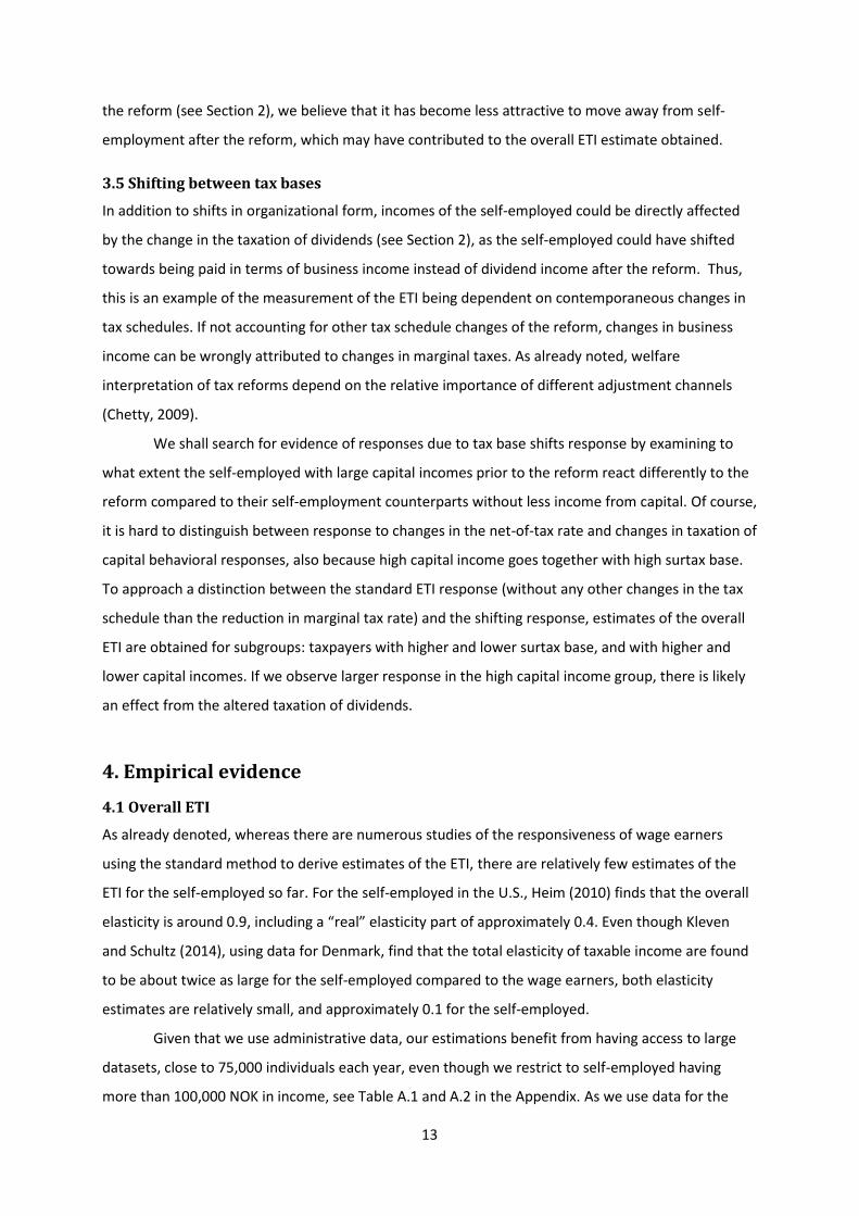
In Table 1 we present estimation results for five different specifications. As expected, OLS
estimation and IV-estimation without any mean reversion control give negative ETI estimates.
Estimation results for Equations 3.2–3.4 (see Section 3) are reported in columns (3)–(5) in Table 1,
demonstrating that results to some extent are sensitive with respect to the mean reversion control
technique used.21 However, all estimates point to relatively small effects, in the range from 0.09 to
0.15. Our estimates are not far from what Kleven and Schultz (2014) found for Denmark.22 Similar to
them, we find results which indicate that the self-employed are somewhat more tax responsive than
the wage earners, when using the results of Thoresen and Vattø (2015) as evidence for the wage
earners.
Table 1. Overall ETI estimation results
(1) (2) (3) (4) (5) OLS IV Auten-Carroll Gruber-Saez Kopczuk Net-of-tax rate -2.635*** -0.963*** 0.123*** 0.091*** 0.152*** (0.008) (0.013) (0.016) (0.016) (0.016) Socioeconomic x x x x x Educational level x x x x x Educational field x x x x x County x x x x x Year x x x x x Instrument x x x x Base year x x x Splines x x N 488283 488258 488258 488258 416735
Standard errors in parentheses, accounted for clustering * p<0.10, ** p<0.05, *** p<0.01
21 Application of instrumentation method of Weber (2014), although with standard controls for mean reversion, gives similar results to those reported in Table 1. 22 A large number of sensitivity tests have been carried out.
15
4.2 Estimation results for working hours
As explained in Section 3, due to constraints in the access to information about hours of work for the
self-employed, in this part of the analysis we use information from repeated cross-sections for the
time period 2001–2010, obtained from the Labor force survey (Statistics Norway, 2003). As the Labor
force survey consists of approximately 22,000 observations per year, it follows that the evidence with
respect to responses in working hours for the self-employed is based on relatively small sample sizes.
As these data do not contain any (usable) panel dimension, estimates of responses in working hours
are obtained by dividing the sample into “experimental group” and “control group” and by using a
standard difference-in-differences estimation technique on groups in cross-sections, see Equation
3.5. The difference in the net-of-tax rates, obtained from the panel data ETI estimation, is used in the
allocation into experimental and control groups.23 Any individual that experienced an increase in the
net-of-tax rate, according to this measure, belongs to the experimental group. They are compared to
self-employed who experience no changes or a reduction in the net-of-tax rates. In two specifications
we also include wage earners with no tax changes in the control group. More information about the
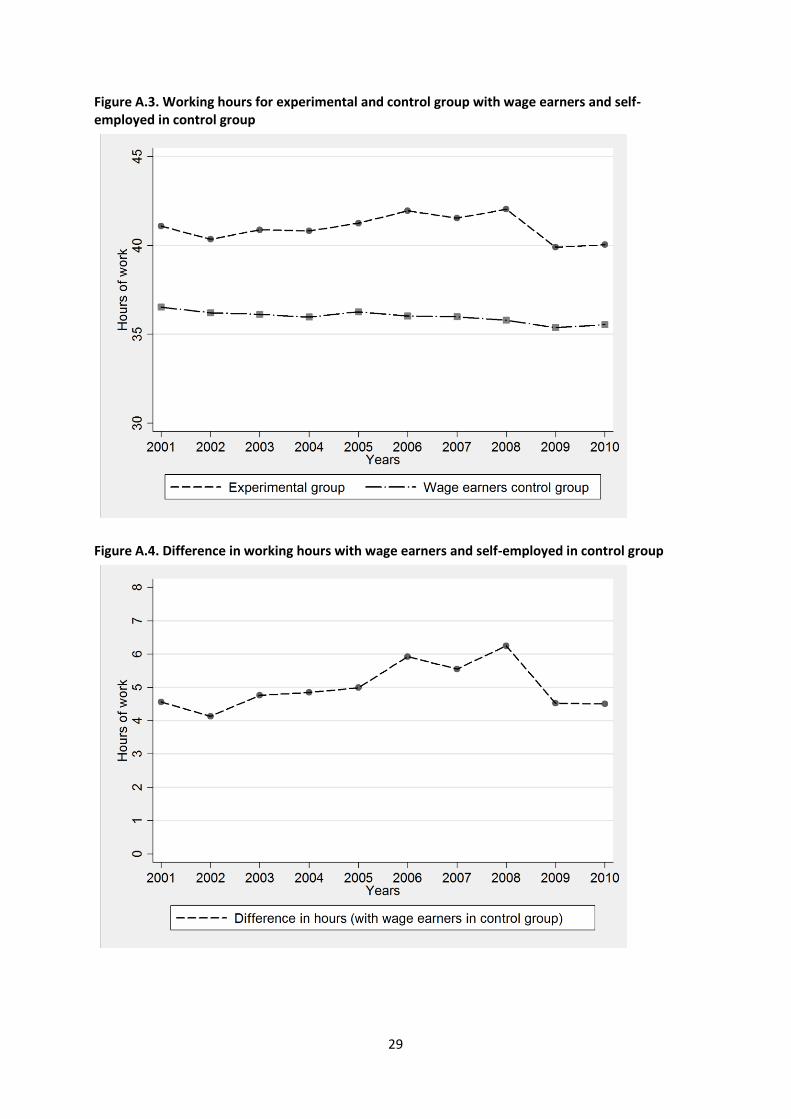
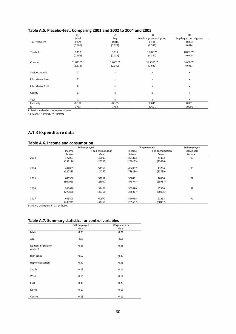
data is provided in the Appendix; see Table A.3 and A.4, and Figures A.1–A.4.
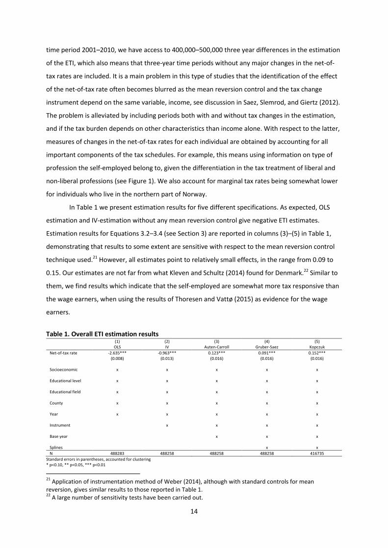
Table 2 presents response estimates for four alternative specifications, which vary with
respect to sample definition and whether the dependent variable is measured in log or level. The
estimated response elasticities range from 0.13 to 0.17, but only the estimate in column (4) is
significantly different from zero. Thus, only when adding wage earners to the control group, we
obtain a significant result. However, all point estimates suggest relatively modest responses, and are
rather close to the estimates of the overall ETI.24
Thus, these results suggest that a large part of the response in the overall ETI is due to real
responses in working hours. However, this does not mean that there are no effects form other
response margins, as they may work in different directions, as we will return to soon.
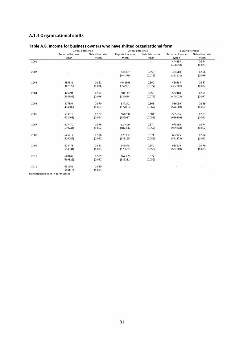
23 These measures can be added to the observations of the Labor force survey through personal identification numbers. 24 Results of a so-called placebo test is presented in Table A.5 in the Appendix, showing no indication of treatment effects outside the reform period.
16
Table 2. Estimation results for working hours (1) (2) (3) (4) Level Log Level-large control group Log–large control group Tax treatment 0.481 0.016 0.468 0.017* (0.585) (0.015) (0.371) (0.010) Treated 0.232 0.007 3.841*** 0.087*** (0.443) (0.011) (0.270) (0.007) Constant 28.056*** 3.381*** 35.795*** 3.592*** (3.821) (0.098) (0.792) (0.022) Socioeconomic X x x x Educational level X x x x Educational field X x x x County X x x x Year X x x x Elasticity 0.130 0.169 0.126 0.166 N 3664 3664 64900 64900
Robust standard errors in parentheses * p<0.10, ** p<0.05, *** p<0.01
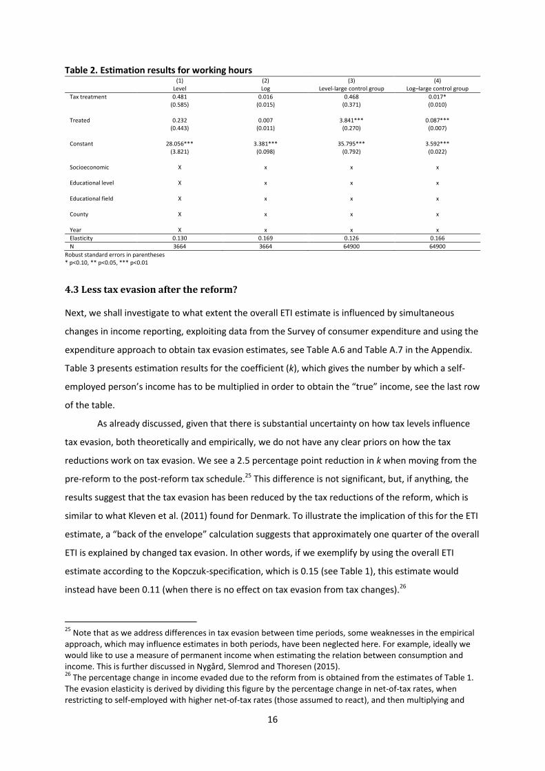
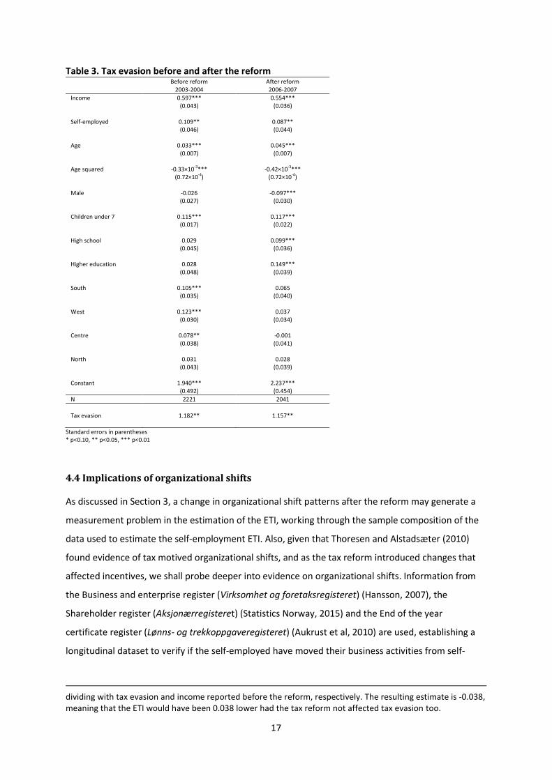
4.3 Less tax evasion after the reform?
Next, we shall investigate to what extent the overall ETI estimate is influenced by simultaneous
changes in income reporting, exploiting data from the Survey of consumer expenditure and using the
expenditure approach to obtain tax evasion estimates, see Table A.6 and Table A.7 in the Appendix.
Table 3 presents estimation results for the coefficient (k), which gives the number by which a self-
employed person’s income has to be multiplied in order to obtain the “true” income, see the last row
of the table.
As already discussed, given that there is substantial uncertainty on how tax levels influence
tax evasion, both theoretically and empirically, we do not have any clear priors on how the tax
reductions work on tax evasion. We see a 2.5 percentage point reduction in k when moving from the
pre-reform to the post-reform tax schedule.25 This difference is not significant, but, if anything, the
results suggest that the tax evasion has been reduced by the tax reductions of the reform, which is
similar to what Kleven et al. (2011) found for Denmark. To illustrate the implication of this for the ETI
estimate, a “back of the envelope” calculation suggests that approximately one quarter of the overall
ETI is explained by changed tax evasion. In other words, if we exemplify by using the overall ETI
estimate according to the Kopczuk-specification, which is 0.15 (see Table 1), this estimate would
instead have been 0.11 (when there is no effect on tax evasion from tax changes).26
25 Note that as we address differences in tax evasion between time periods, some weaknesses in the empirical approach, which may influence estimates in both periods, have been neglected here. For example, ideally we would like to use a measure of permanent income when estimating the relation between consumption and income. This is further discussed in Nygård, Slemrod and Thoresen (2015). 26 The percentage change in income evaded due to the reform from is obtained from the estimates of Table 1. The evasion elasticity is derived by dividing this figure by the percentage change in net-of-tax rates, when restricting to self-employed with higher net-of-tax rates (those assumed to react), and then multiplying and
17
Table 3. Tax evasion before and after the reform Before reform
2003-2004 After reform 2006-2007
Income 0.597*** 0.554*** (0.043) (0.036) Self-employed 0.109** 0.087** (0.046) (0.044) Age 0.033*** 0.045*** (0.007) (0.007) Age squared -0.33×10⁻³*** -0.42×10⁻³*** (0.72×10⁻⁴) (0.72×10⁻⁴) Male -0.026 -0.097*** (0.027) (0.030) Children under 7 0.115*** 0.117*** (0.017) (0.022) High school 0.029 0.099*** (0.045) (0.036) Higher education 0.028 0.149*** (0.048) (0.039) South 0.105*** 0.065 (0.035) (0.040) West 0.123*** 0.037 (0.030) (0.034) Centre 0.078** -0.001 (0.038) (0.041) North 0.031 0.028 (0.043) (0.039) Constant 1.940*** 2.237*** (0.492) (0.454) N 2221 2041 Tax evasion 1.182** 1.157**
Standard errors in parentheses * p<0.10, ** p<0.05, *** p<0.01
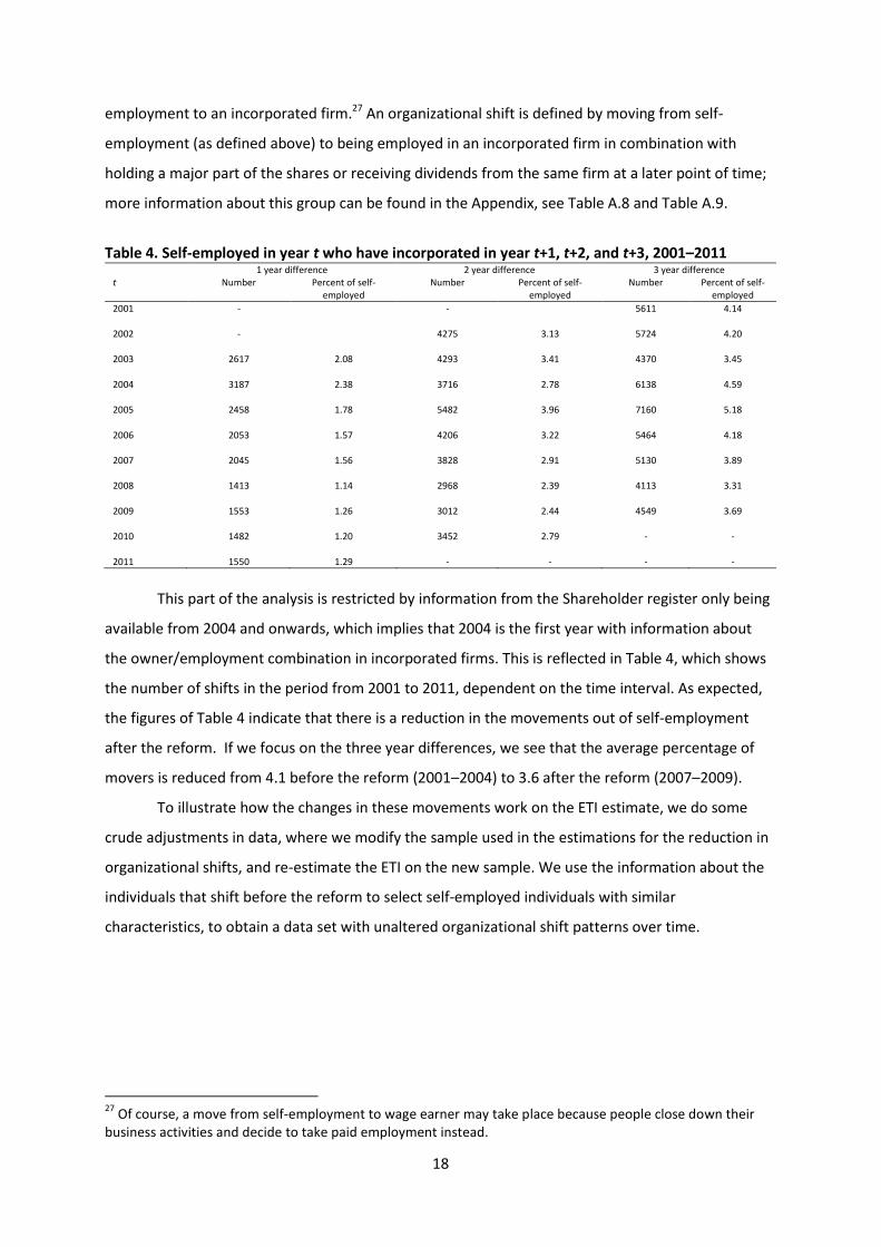
4.4 Implications of organizational shifts
As discussed in Section 3, a change in organizational shift patterns after the reform may generate a
measurement problem in the estimation of the ETI, working through the sample composition of the
data used to estimate the self-employment ETI. Also, given that Thoresen and Alstadsæter (2010)
found evidence of tax motived organizational shifts, and as the tax reform introduced changes that
affected incentives, we shall probe deeper into evidence on organizational shifts. Information from
the Business and enterprise register (Virksomhet og foretaksregisteret) (Hansson, 2007), the
Shareholder register (Aksjonærregisteret) (Statistics Norway, 2015) and the End of the year
certificate register (Lønns- og trekkoppgaveregisteret) (Aukrust et al, 2010) are used, establishing a
longitudinal dataset to verify if the self-employed have moved their business activities from self-
dividing with tax evasion and income reported before the reform, respectively. The resulting estimate is -0.038, meaning that the ETI would have been 0.038 lower had the tax reform not affected tax evasion too.
18
employment to an incorporated firm.27 An organizational shift is defined by moving from self-
employment (as defined above) to being employed in an incorporated firm in combination with
holding a major part of the shares or receiving dividends from the same firm at a later point of time;
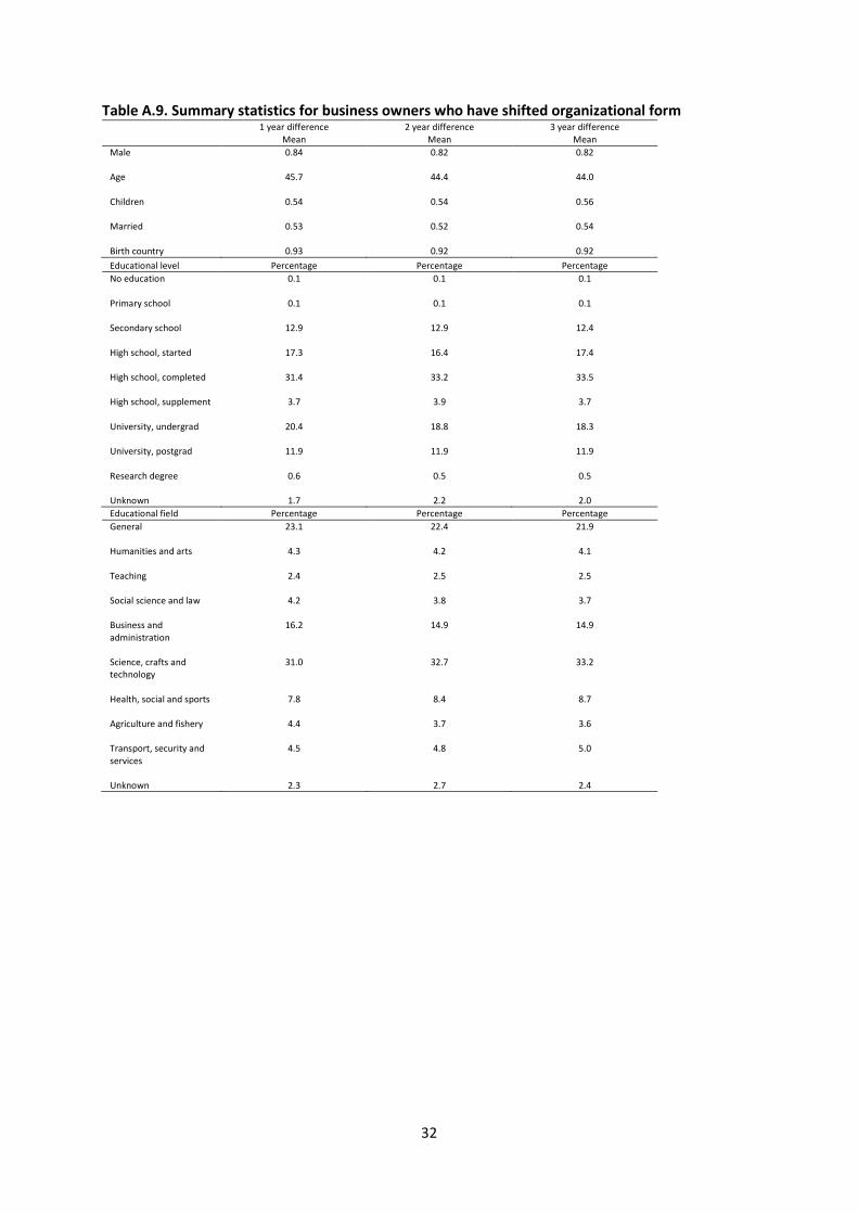
more information about this group can be found in the Appendix, see Table A.8 and Table A.9.
Table 4. Self-employed in year t who have incorporated in year t+1, t+2, and t+3, 2001–2011
1 year difference 2 year difference 3 year difference t Number Percent of self-
employed Number Percent of self-
employed Number Percent of self-
employed 2001 - - 5611 4.14 2002 - 4275 3.13 5724 4.20 2003 2617 2.08 4293 3.41 4370 3.45 2004 3187 2.38 3716 2.78 6138 4.59 2005 2458 1.78 5482 3.96 7160 5.18 2006 2053 1.57 4206 3.22 5464 4.18 2007 2045 1.56 3828 2.91 5130 3.89 2008 1413 1.14 2968 2.39 4113 3.31 2009 1553 1.26 3012 2.44 4549 3.69 2010 1482 1.20 3452 2.79 - - 2011 1550 1.29 - - - -
This part of the analysis is restricted by information from the Shareholder register only being
available from 2004 and onwards, which implies that 2004 is the first year with information about
the owner/employment combination in incorporated firms. This is reflected in Table 4, which shows
the number of shifts in the period from 2001 to 2011, dependent on the time interval. As expected,
the figures of Table 4 indicate that there is a reduction in the movements out of self-employment
after the reform. If we focus on the three year differences, we see that the average percentage of
movers is reduced from 4.1 before the reform (2001–2004) to 3.6 after the reform (2007–2009).
To illustrate how the changes in these movements work on the ETI estimate, we do some
crude adjustments in data, where we modify the sample used in the estimations for the reduction in
organizational shifts, and re-estimate the ETI on the new sample. We use the information about the
individuals that shift before the reform to select self-employed individuals with similar
characteristics, to obtain a data set with unaltered organizational shift patterns over time.
27 Of course, a move from self-employment to wage earner may take place because people close down their business activities and decide to take paid employment instead.
19
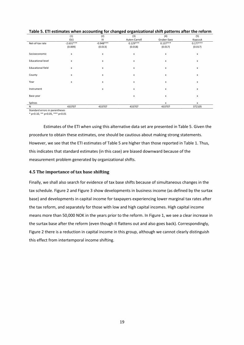
Table 5. ETI estimates when accounting for changed organizational shift patterns after the reform (1) (2) (3) (4) (5) OLS IV Auten-Carroll Gruber-Saez Kopczuk Net-of-tax rate -2.631*** -0.948*** 0.129*** 0.137*** 0.177*** (0.009) (0.013) (0.018) (0.017) (0.017) Socioeconomic x x x x x Educational level x x x x x Educational field x x x x x County x x x x x Year x x x x x Instrument x x x x Base year x x x Splines x x N 433707 433707 433707 433707 372105 Standard errors in parentheses * p<0.10, ** p<0.05, *** p<0.01
Estimates of the ETI when using this alternative data set are presented in Table 5. Given the
procedure to obtain these estimates, one should be cautious about making strong statements.
However, we see that the ETI estimates of Table 5 are higher than those reported in Table 1. Thus,
this indicates that standard estimates (in this case) are biased downward because of the
measurement problem generated by organizational shifts.
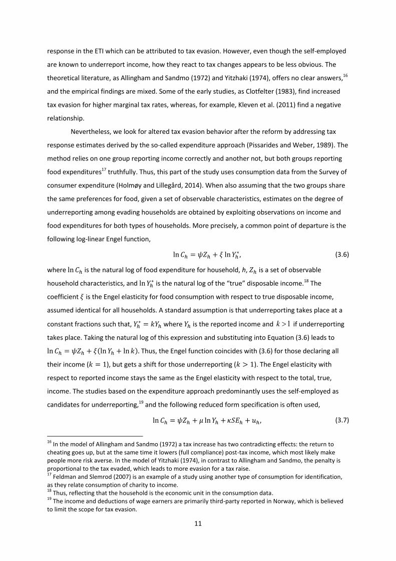
4.5 The importance of tax base shifting
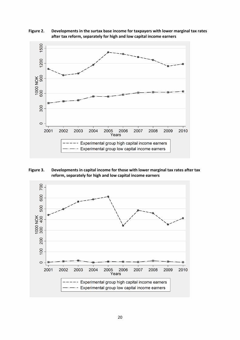
Finally, we shall also search for evidence of tax base shifts because of simultaneous changes in the
tax schedule. Figure 2 and Figure 3 show developments in business income (as defined by the surtax
base) and developments in capital income for taxpayers experiencing lower marginal tax rates after
the tax reform, and separately for those with low and high capital incomes. High capital income
means more than 50,000 NOK in the years prior to the reform. In Figure 1, we see a clear increase in
the surtax base after the reform (even though it flattens out and also goes back). Correspondingly,
Figure 2 there is a reduction in capital income in this group, although we cannot clearly distinguish
this effect from intertemporal income shifting.
20
Figure 2. Developments in the surtax base income for taxpayers with lower marginal tax rates after tax reform, separately for high and low capital income earners
Figure 3. Developments in capital income for those with lower marginal tax rates after tax reform, separately for high and low capital income earners
21
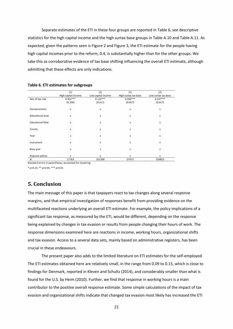
Separate estimates of the ETI in these four groups are reported in Table 6, see descriptive
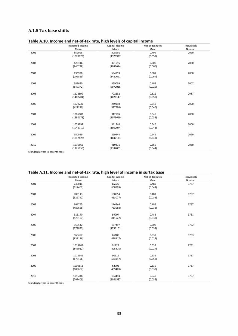
statistics for the high capital income and the high surtax base groups in Table A.10 and Table A.11. As
expected, given the patterns seen is Figure 2 and Figure 3, the ETI estimate for the people having
high capital incomes prior to the reform, 0.4, is substantially higher than for the other groups. We
take this as corroborative evidence of tax base shifting influencing the overall ETI estimate, although
admitting that these effects are only indications.
Table 6. ETI estimates for subgroups (1) (2) (1) (2) High capital income Low capital income High surtax tax base Low surtax tax base Net-of-tax rate 0.401*** 0.124*** 0.200*** 0.147*** (0.100) (0.017) (0.057) (0.017) Socioeconomic x x x x Educational level x x x x Educational field x x x x County x x x x Year x x x x Instrument x x x x Base year x x x x Kopczuk splines x x x x N 17763 351309 57473 316853
Standard errors in parentheses, accounted for clustering
* p<0.10, ** p<0.05, *** p<0.01
5. Conclusion The main message of this paper is that taxpayers react to tax changes along several response
margins, and that empirical investigation of responses benefit from providing evidence on the
multifaceted reactions underlying an overall ETI estimate. For example, the policy implications of a
significant tax response, as measured by the ETI, would be different, depending on the response
being explained by changes in tax evasion or results from people changing their hours of work. The
response dimensions examined here are reactions in income, working hours, organizational shifts
and tax evasion. Access to a several data sets, mainly based on administrative registers, has been
crucial in these endeavours.
The present paper also adds to the limited literature on ETI estimates for the self-employed.
The ETI estimates obtained here are relatively small, in the range from 0.09 to 0.15, which is close to
findings for Denmark, reported in Kleven and Schultz (2014), and considerably smaller than what is
found for the U.S. by Heim (2010). Further, we find that response in working hours is a main
contributor to the positive overall response estimate. Some simple calculations of the impact of tax
evasion and organizational shifts indicate that changed tax evasion most likely has increased the ETI
22
estimate, whereas more people remaining in self-employment after the reform, due to fewer
organizational shifts, implies that the ETI is smaller than it otherwise would have been. We also see
some indications of the overall ETI estimate being influenced by other (simultaneous) changes in the
tax schedule, i.e., shifting across tax bases.
References Aarbu, Karl O., Thor O. Thoresen (2001). “Income Responses to Tax Changes – Evidence from the
Norwegian Tax Reform”, National Tax Journal 54(2): 319–338.
Allingham, Michael, Agnar Sandmo (1972). “Income Tax Evasion: A Theoretical Analysis”, Journal of
Public Economics 1(3): 323–338.
Alstadsæter, Annette, Erik Fjærli (2009). “Neutral Taxation of Shareholder Income? Corporate
Responses to an Announced Dividend Tax”, International Tax and Public Finance 16: 571–
604.
Angrist, Joshua D., Jörn-Steffen Pischke (2009). “Mostly Harmless Econometrics – An Empiricist’s
Companion”, Princeton and Oxford: Princeton University Press.
Aukrust, Inge, Per Svein Aurdal, Magne Bråthen, Tonje Køber (2010). “Registerbasert
sysselsettingsstatistikk. Dokumentasjon”, Notater 8/2010, Statistics Norway.
Auten, Gerald, Robert Carroll (1999). “The Effect of Income Taxes on Household Income”, Review of
Economics and Statistics 81(4): 681–693.
Bastani, Spencer, Håkan Selin (2014). “Bunching and Non-Bunching at Kink Points of the Swedish Tax
Schedule”, Journal of Public Economics 109: 36–49.
Blomquist, Søren, Håkan Selin (2010). “Hourly Wage Rate and Taxable Labor Income
Responsiveness to Changes in Marginal Tax Rates”, Journal of Public Economics, 94: 878–889.
Blow, Laura, Ian Preston (2002). “Deadweight Loss and Taxation of Earned Income: Evidence from
Tax Records of the UK Self-Employed”, IFS Working Paper.
Chetty, Raj (2009). “Is the Taxable Income Elasticity Sufficient to Calculate Deadweight Loss? The
Implications of Evasion and Avoidance”, American Economic Journal: Economic Policy 1(2):
31–52.
Chetty, Raj (2012). “Bounds on Elasticities with Optimization Frictions: A Synthesis of Micro
and Macro Evidence on Labor Supply”, Econometrica 80(3): 969–1018.
Christansen, Vidar (2004). “Norwegian Income Tax Reforms”, CESifo DICE Report, 3/2004: 9–14.
Clotfelter, Charles T. (1983). “Tax Evasion and Tax Rates: An Analysis of Individual Returns”, Review of
Economics and Statistics, 65(3): 363–373.
23
Edmark, Karin, Roger H. Gordon, (2013). “The Choice of Organizational form by Closely-Held Firms in
Sweden: Tax versus non-Tax Determinants”, Industrial and Corporate Change 22(1): 219–243
Engström, Per, Bertil Holmlund (2009). “Tax evasion and self-employment in a high-tax country:
evidence from Sweden”, Applied Economics 41(19): 2419–2430.
Feldman, Naomi, Joel Slemrod (2007). “Estimating Tax Noncompliance with Evidence from
Unaudited Tax Returns”, Economic Journal 117(3): 327–352.
Feldstein, Martin (1995). “The Effect of Marginal Tax Rates on Taxable Income: A Panel Study of the
1986 Tax Reform Act”, Journal of Political Economy 303(3): 551–572.
Feldstein, Martin (1999). “Tax Avoidance and the Deadweight loss of the Income Tax”, Review of
Economics and Statistics 81(4): 674–680.
Gordon, Roger H., Joel B. Slemrod. (2000). “Are ‘Real’ Responses to Taxes Simply Income Shifting
Between Corporate and Personal Tax Bases?”, in Joel Slemrod (Ed.), Does Atlas Shrug? The
Economic Consequences of Taxing the Rich, Cambridge: Harvard University Press, 240–281.
Goolsbee, Austan (1999). “Evidence on the High–Income Laffer Curve from Six Decades of Tax
Reforms”, Brookings Papers on Economic Activity No. 2 (1999): 1–47.
Gruber, Jon, Emmanuel Saez (2002). “The Elasticity of Taxable Income: Evidence and Implications”,
Journal of Public Economics 84(1): 1–32.
Hansson, Ann-Kristin (2007). “Bedrifts- og foretaksregisteret. Regler og rutiner for ajourhold av Bof”,
Notater 2/2007, Statistics Norway.
Heim, Bradley T. (2010). “The responsiveness of self-employment income to tax rate changes”,
Journal of Labor Economics 17(6): 940–950.
Holmøy, Aina, Magnar Lillegård (2014). “Forbruksundersøkelsen 2012. Dokumentasjonsrapport”.
Notater 2014/17. Statistcs Norway.
Johansson, Edvard (2005). “An estimate of self-employment income underreporting in Finland”,
Nordic Journal of Political Economy 31: 99–109.
Kleven, Henrik J., Martin B. Knudsen, Claus T. Kreiner, Søren Pedersen, Emmanuel Saez (2011).
“Unwilling or Unable to Cheat? Evidence from a Tax Audit Experiment in Denmark“,
Econometrica 79(3): 651–692.
Kleven, Henrik J., Esben A. Schultz (2014). “Estimating Taxable Income Responses Using Danish Tax
Reforms“, American Economic Journal: Economic Policy 6(4): 271–301.
Kopczuk, Wojciech (2005). “Tax Bases, Tax Rates and the Elasticity of Reported Income”, Journal of
Public Economics 89: 2093–2119.
Le Maire, Daniel, Bertel Scherning (2013), “Tax Bunching, Income Shifting and Self-Employment”,
Journal of Public Economics 107: 1–18.
24
Lindsey, Lawrence B. (1987). “Individual Taxpayer Responses to Tax Cuts: 1982-1984: With
Implications for the Revenue Maximizing Tax Rate”, Journal of Public Economics 33(2): 173–
206.
Nygård, Odd Erik, Joel Slemrod, and Thor O. Thoresen (2015). “Distributional Implication of Joint Tax
Evasion”, manuscript, Statistics Norway.
Pissarides, Christopher A., Guglielmo Weber (1989). “An Expenditure-Based Estimate of Britain’s
Black Economy”, Journal of Public Economics 39(1): 17–32.
Saez, Emmanuel, Joel Slemrod, and Seth H. Giertz (2012). "The Elasticity of Taxable Income with
Respect to Marginal Tax Rates: A Critical Review" Journal of Economic Literature 50(1): 3–50.
Slemrod, Joel (1995). “Income Creation or Income Shifting? Behavioral Responses to the Tax Reform
Act of 1986,” American Economic Review Papers and Proceedings, 85(2), 175–180.
Slemrod, Joel (1996). “High-Income Families and the Tax Changes of the 1980s: The Anatomy of
Behavioral Response”. In Martin Feldstein and James Poterba (Eds.), Empirical Foundations of
Household Taxation, University of Chicago Press, 169–192.
Slemrod, Joel (2007). “Cheating Ourselves: The Economics of Tax Evasion”, Journal of Economic
Perspectives 21 (1): 25–48.
Statistics Norway (2003). “Labour Force Survey 2001”, Official Statistics of Norway.
Statistics Norway (2005). “Income Statistics for Persons and Families 2002–2003”, Official Statistics
of Norway.
Statistics Norway (2015). http://www.ssb.no/en/virksomheter-foretak-og-
regnskap/statistikker/aksjer/aar-forelopige/2015-06-26.
Thoresen, Thor O., Annette Alstadsæter (2010). “Shifts in Organizational Form under a Dual Income
Tax System”, FinanzArchiv: Public Finance Analysis 66(4): 384–418.
Thoresen, Thor O., Trine E. Vattø (2015). “Validation of the Discrete Choice Labor Supply Model by
Methods of the New Tax Responsiveness Literature”, Statistics Norway Discussion Paper.
Weber, Caroline (2014). Toward Obtaining a Consistent Estimate of the Elasticity of Taxable Income
Using Difference-in-Differences, Journal of Public Economics, 117, 90–103.
Wu, Shih-Ying (2005). “The Effect on Taxable Income from Privately Held Businesses”, Southern
Economic Journal, 71(4): 891–912.
Yitzhaki, Shlomo (1974). “A Note on Income Tax Evasion: A Theoretical Analysis”, Journal of
Public Economics, 3(2): 201–202.
25
Appendix
A.1 Summary statistics
A.1.1 Income data Table A.1. Income and net-of-tax rates
Reported income Net-of-tax rates Self-employed individuals Mean Mean Number 2001 299782 0.576 71353 (307815) (0.074) 2002 316467 0.583 72590 (290482) (0.073) 2003 317794 0.589 72103 (293629) (0.072) 2004 377000 0.584 74257 (316001) (0.073) 2005 397739 0.594 74749 (391337) (0.063) 2006 431448 0.601 76220 (421270) (0.050) 2007 468548 0.595 77781 (436927) (0.052) 2008 452082 0.597 77380 (393619) (0.052) 2009 451961 0.600 77485 (406667) (0.051) 2010 469104 0.600 77701 (427944) (0.051)
mean coefficients; sd in parentheses
26
Table A.2. Summary statistics for control variables Characteristics Mean Educational level Percentage in sample Educational field Percentage in sample Male 0.75 No education 0.1 General 31.2 Age 46.0 Primary school 0.1 Humanities and arts 4.5 Children 0.59 Secondary school 19.8 Teaching 2.1 Married 0.57 High school, started 25.5 Social science and
law 3.4
Birth country 0.93 High school, completed 28.8 Business and
administration 9.3
High school, supplement 2.4 Science, crafts and
technology 24.9
University, undergrad 12.5 Health, social and
sports 11.5
University postgrad 9.18 Agriculture and
fishery 5.5
Research degree 0.3 Transport, security
and services 5.6
Unknown 1.3 Unknown 1.8
A.1.2 Working hours data Table A.3. Hours of work
Treated Control 1 Control 2 Hours of work Net-of-tax rate Hours of work Net-of-tax rate Hours of work Net-of-tax rate Before reform 41.3 0.517 42.2 0.618 36.2 0.625 (9.1) (0.055) (9.6) (0.053) (6.3) (0.047) After reform 40.7 0.558 41.0 0.615 35.7 0.624 (9.1) (0.043) (9.7) (0.044) (6.6) (0.038)
Mean coefficients, standard deviations in parentheses
27
Table A.4. Summary statistics for control variables Experimental group Small control group Large control group Mean Mean Mean Male 0.80 0.78 0.49 Age 48.0 47.3 40.9 Child 0.63 0.61 0.57 Married 0.61 0.62 0.50 Birth country 0.93 0.95 0.94
Educational level Experimental group Small control group Large control group Percentage Percentage Percentage No education 0.0 0.0 0.1 Primary school 0.1 0.0 0.1 Secondary school 15.0 20.3 14.3 High school, started 16.2 30.9 18.5 High school, completed High school, supplement University, undergrad University, postgrad Research degree Unknown
24.3
2.0
18.0
22.0
0.7
1.7
33.3
2.6
9.1
3.5
0.0
0.5
34.0
3.4
28.8
3.7
0.2
0.9
Educational field Experimental group Small control group Large control group Percentage Percentage Percentage General 22.6 34.8 24.5 Humanities and arts 4.2 3.8 4.4 Teaching 2.2 2.3 7.5 Social science and law 7.4 1.2 2.2 Business and administration Science, crafts and technology Health, social and sports Agriculture and fishery Transport, security and services Unknown
8.7
21.6
24.9
3.0
3.5
2.0
11.2
30.0
5.6
4.7
5.6
0.9
13.9
26.1
15.6
1.1
3.1
1.5
28
Figure A.1. Working hours for experimental and control group with only self-employed in control group
Figure A.2. Difference in working hours with only self-employed in control group
29
Figure A.3. Working hours for experimental and control group with wage earners and self-employed in control group
Figure A.4. Difference in working hours with wage earners and self-employed in control group
30
Table A.5. Placebo-test. Comparing 2001 and 2002 to 2004 and 2005 (1) (2) (3) (4) Level Log Level-large control group Log–large control group Tax treatment -0.571 -0.015 0.181 0.003 (0.860) (0.022) (0.539) (0.014) Treated 0.412 0.012 3.782*** 0.087*** (0.591) (0.015) (0.357) (0.009) Constant 31.812*** 3.460*** 38.737*** 3.660*** (5.516) (0.140) (1.089) (0.031) Socioeconomic X x x x Educational level X x x x Educational field X x x x County X x x x Year X x x x Elasticity -0.152 -0.165 0.049 0.031 N 1763 1763 30501 30501
Robust standard errors in parentheses * p<0.10, ** p<0.05, *** p<0.01
A.1.3 Expenditure data Table A.6. Income and consumption
Self-employed Wage earners Self-employed Income Food consumption Income Food consumption individuals Mean Mean Mean Mean Number 2003 472001 49013 454463 44432 99 (239176) (25259) (250193) (23896) 2004 494889 51956 484997 43204 95 (220883) (24270) (779194) (22739) 2005 680560 52252 508431 46586 77 (967065) (28047) (478743) (25987) 2006 542039 57406 503499 47970 83 (270838) (32358) (266367) (28095) 2007 653805 60977 550958 51493 90 (440945) (41758) (285587) (30057)
Standard deviations in parentheses Table A.7. Summary statistics for control variables
Self-employed Wage earners Mean Mean Male 0.75 0.71 Age 46.8 46.1 Number of children under 7
0.35 0.38
High school 0.52 0.49 Higher education 0.30 0.36 South 0.13 0.14 West 0.19 0.17 East 0.30 0.29 North 0.10 0.13 Centre 0.13 0.11
31
A.1.4 Organizational shifts Table A.8. Income for business owners who have shifted organizational form
1 year difference 2 year difference 3 year difference Reported income Net-of-tax rates Reported income Net-of-tax rates Reported income Net-of-tax rates Mean Mean Mean Mean Mean Mean 2001 - - - - 444254 0.544 (450510) (0.073) 2002 - - 446307 0.553 434569 0.556 (444379) (0.076) (361171) (0.076) 2003 435131 0.561 4441696 0.560 460684 0.557 (342879) (0.076) (352901) (0.077) (362801) (0.077) 2004 475294 0.557 501147 0.553 502460 0.554 (394847) (0.076) (422634) (0.076) (445025) (0.077) 2005 527857 0.570 537242 0.568 536059 0.569 (454809) (0.067) (577083) (0.067) (574669) (0.067) 2006 534519 0.587 561280 0.584 565636 0.583 (672008) (0.051) (682917) (0.051) (639809) (0.051) 2007 617470 0.576 624409 0.574 675159 0.574 (659741) (0.052) (682356) (0.052) (939840) (0.052) 2008 625217 0.576 676382 0.574 652925 0.574 (616047) (0.052) (689165) (0.052) (571878) (0.052) 2009 672478 0.581 643848 0.580 638629 0.579 (654334) (0.053) (578687) (0.053) (507689) (0.053) 2010 640147 0.579 667399 0.577 - - (669822) (0.052) (586281) (0.052) 2011 691551 0.580 - - - - (564110) (0.053)
Standard deviations in parentheses
32
Table A.9. Summary statistics for business owners who have shifted organizational form 1 year difference 2 year difference 3 year difference Mean Mean Mean Male 0.84 0.82 0.82 Age 45.7 44.4 44.0 Children 0.54 0.54 0.56 Married 0.53 0.52 0.54 Birth country 0.93 0.92 0.92
Educational level Percentage Percentage Percentage No education 0.1 0.1 0.1 Primary school 0.1 0.1 0.1 Secondary school 12.9 12.9 12.4 High school, started 17.3 16.4 17.4 High school, completed High school, supplement University, undergrad University, postgrad Research degree Unknown
31.4
3.7
20.4
11.9
0.6
1.7
33.2
3.9
18.8
11.9
0.5
2.2
33.5
3.7
18.3
11.9
0.5
2.0
Educational field Percentage Percentage Percentage General 23.1 22.4 21.9 Humanities and arts 4.3 4.2 4.1 Teaching 2.4 2.5 2.5 Social science and law 4.2 3.8 3.7 Business and administration Science, crafts and technology Health, social and sports Agriculture and fishery Transport, security and services Unknown
16.2
31.0
7.8
4.4
4.5
2.3
14.9
32.7
8.4
3.7
4.8
2.7
14.9
33.2
8.7
3.6
5.0
2.4
33
A.1.5 Tax base shifts Table A.10. Income and net-of-tax rate, high levels of capital income
Reported income Capital income Net-of-tax rates Individuals Mean Mean Mean Number 2001 852065 308591 0.499 2060 (1079629) (1370927) (0.059) 2002 820416 401615 0.506 2060 (840738) (1087694) (0.066) 2003 836990 584113 0.507 2060 (796559) (1480621) (0.064) 2004 982620 599099 0.482 2007 (842372) (2072016) (0.029) 2005 1122599 702232 0.522 2037 (1402704) (4026147) (0.052) 2006 1079232 249110 0.549 2020 (421270) (927780) (0.040) 2007 1085802 312576 0.545 2038 (1380178) (1073619) (0.039) 2008 1059292 341540 0.546 2060 (1041310) (1802044) (0.041) 2009 980989 229444 0.549 2060 (1047123) (1047123) (0.043) 2010 1015565 419871 0.550 2060 (1125656) (2334001) (0.044)
Standard errors in parentheses Table A.11. Income and net-of-tax rate, high level of income in surtax base
Reported income Capital income Net-of-tax rates Individuals Mean Mean Mean Number 2001 739011 85320 0.489 9787 (612401) (658599) (0.044) 2002 788113 100654 0.482 9787 (522742) (463077) (0.033) 2003 864755 144844 0.482 9787 (482658) (733068) (0.033) 2004 916140 95294 0.481 9761 (526157) (811522) (0.033) 2005 950512 137497 0.509 9762 (772833) (1793101) (0.034) 2006 960457 66185 0.539 9733 (832186) (478417) (0.027) 2007 1013969 91821 0.534 9731 (848912) (495475) (0.027) 2008 1012546 90316 0.536 9787 (678156) (583147) (0.052) 2009 1000615 62706 0.539 9787 (608657) (499489) (0.033) 2010 1015800 154494 0.540 9787 (707409) (2081587) (0.035)
Standard errors in parentheses