Embed Size (px)
Citation preview

Improving Electron Micrograph Signal-to-Noise with an Atrous ConvolutionalEncoder-Decoder
Jeffrey M. Ede
Abstract: We present an atrous convolutional encoder-decoder trained to denoise 512×512 crops from electronmicrographs. It consists of a modified Xception backbone,atrous convoltional spatial pyramid pooling moduleand a multi-stage decoder. Our neural network wastrained end-to-end to remove Poisson noise appliedto low-dose (� 300 counts ppx) micrographs createdfrom a new dataset of 17267 2048×2048 high-dose (>2500 counts ppx) micrographs and then fine-tuned forordinary doses (200-2500 counts ppx). Its performanceis benchmarked against bilateral, non-local means, totalvariation, wavelet, Wiener and other restoration methodswith their default parameters. Our network outperformstheir best mean squared error and structural similarityindex performances by 24.6% and 9.6% for low dosesand by 43.7% and 5.5% for ordinary doses. In bothcases, our network’s mean squared error has the lowestvariance. Source code and links to our new high-qualitydataset and trained network have been made publiclyavailable at https://github.com/Jeffrey-Ede/Electron-Micrograph-Denoiser.
Keywords: deep learning, denoising, electron microscopy,low dose
1 Introduction
Every imaging mode in electron microscopy is limitedby and has been shaped by noise[1]. Increasingly, evermore sophisticated and expensive hardware and softwarebased methods are being developed to increase resolution,including aberration correctors[2, 3], advanced cold fieldemission guns[4, 5], holography[6, 7] and others[8–10].However, these developments are all fundamentally limitedby the signal-to-noise ratios in the micrographs theyare being applied to. Low-dose applications such assingle-particle cryogenic microscopy[11] and real-timetomography[9] are also complicated, made preventivelydifficult or limited by noise.
Moving towards higher resolution, a large number
of general[12] and electron microscopy-specific[1, 13]denoising algorithms have been developed. However,most of these algorithms rely on laboriously hand-craftedfilters and are rarely; if ever, truly optimized for theirtarget domains e.g. [14]. Neural networks are universalapproximators[15] that overcome these difficulties[16]through representation learning[17]. As a result, networksare increasingly being applied to noise removal[18–21] andother applications in electron microscopy[22–25] and otherareas of science.
The recent success of large neural networks in computervision is attributed to the advent of graphical processingunit (GPU) acceleration[26, 27]. In particular, the GPUacceleration of large convolutional neural networks[28, 29](CNNs) in distributed settings[30, 31]. Large networksthat surpass human performance in image classification[32,33], computer games[34–36], speech recognition[37, 38],relational reasoning[39] and in many other applications[23,40–43] have all been enabled by GPUs.
At the time of writing, there are no large neural networksfor electron micrograph denoising. Instead, most denoisingnetworks act on many small overlapping crops e.g. [20].This makes them computationally inefficient and unable toutilize all the information available. Some large denoisingnetworks have been trained as part of generative adversarialnetworks[44] and try to generate micrographs resemblinghigh-quality training data as closely as possible. Thiscan avoid the blurring effect of most filters; however,this is achieved by generating features that might be inhigh-quality micrographs. This means that they are proneto producing artifacts; something that is often undesirablein scientific applications.
This paper presents a large CNN for electron micrographdenoising. Network architecture is shown in section 2. Thecollation of a new high-quality electron micrograph trainingdataset, training hyperparameters and learning protocols aredescribed in section 3. Performance comparison with othermethods’, error characterization and example usage are insection 4. Finally, architecture and hyperparameter tuningexperiments are presented in section 5.
1
arX
iv:1
807.
1123
4v2
[cs
.CV
] 2
Nov
201
8

Figure 1: Architecture of our deep convolutional encoder-decoder for electron micrograph denoising. The entry and middleflows develop high-level features that are sampled at multiple scales by the atrous spatial pyramid pooling module. Thisproduces rich semantic information that is concatenated with low-level entry flow features and resolved into denoisedmicrographs by the decoder.
2

Figure 2: Start of an unmodified Xception entry flow[45].
2 Architecture
Our highest performing denoising network was trained for512×512 inputs and is shown in fig. 1. It consists ofmodified Xception[45] entry and middle flows for featureextraction, an atrous spatial pyramid pooling (ASPP)module[46, 47] that samples rich high-level semantics atmultiple scales and a multi-stage decoder that combineslow-level entry flow features with ASPP semantics toresolve them. The architecture is inspired by Google’sDeepLab3[46], DeepLab3+[47] and other encoder-decoderarchitectures[18, 20, 48]. A guide for readers unfamiliarwith convolution arithmetic for deep learning is [49].
Convolutions all use 3×3 or 1×1 kernels and arefollowed by batch normalization[50] before ReLU6[51]activation. Similar to DeepLab3+, original Xception maxpooling layers have been replaced with strided depthwiseseparable convolutions, enabling the network to learn itsown downsampling. Extra batch normalization is addedbetween the depthwise and pointwise convolutions of everydepthwise separable convolution like in MobileNet[52].
The following subsections correspond to the subsectionsof fig. 1. Training details follow in section 3.
2.1 Entry Flow
Other than the modification of max pooling layers tostrided depthwise separable convolutions, most entry flowconvolutions are similar to Xception’s[45]. Commonconvolutions have the same number of features and arearranged into Xception-style residual[53] blocks to reducesemantic decimation during downsampling[46].
The main change is the replacement of the firsttwo Xception convolutions with an residual convolutionaldownsampling block. For reference, the start of the originalXception entry flow is shown in fig. 2. This changewas made so that the lowest-level features concatenatedin the decoder would be deeper and have a larger featurespace. An alternative solution is to apply additional
pre-concatenation 1×1 convolutions to change the featurespace size. This was the approach taken in DeepLab3+[47]to prevent high-level ASPP semantics being overwhelmedby low-level features in the decoder.
2.2 Middle Flow
Skip-3 residual blocks are repeated 12 times to develophigh-level semantics to flow into the ASPP module. Thisis more than the 8 skip-3 blocks used in Xception[45] asthe inflowing tensors are larger; 32×32×728 rather than19×19×728. Nevertheless, this is fewer than the 16 skip-3residual blocks used in DeepLab3+ for similar tensors[47].Middle flow tensors are much smaller than those in otherparts of the network so this decision was a compromisebetween expressibility and training time.
2.3 Atrous Spatial Pyramid Pooling
This is the ASPP module Google developed for semanticimage segmentation[46, 47] without a pre-pooling 1×1convolution. It is being used rather than a fully connectedlayer; like the one in [18]’s denoiser, to sample semanticsat multiple scales as it requires fewer parameters and hasalmost identical performance. The atrous rates of 6, 12and 18 are the same as those used in the original ASPPmodule[46]. Importantly, a bottleneck 1×1 convolution isused to reduce the number of output features from 3640to 256, forcing the network to work harder to develophigh-level semantics.
2.4 Decoder
Rich ASPP semantics are bilinearly upsampled from32×32×256 to 128×128×256 feature maps andconcatenated with low-level entry flow features toresolve them in the following convolutions. This issimilar to the approach used in other encoder-decoderarchitectures[18, 20, 46–48]. There are two residualconcatenations with low-level features from the entry flow;rather than one, so that semantics can be resolved from thefirst concatenation before being resolved into fine spatialinformation after the second.
To prevent rich semantic information from beingoverwhelmed by low-level features, feature sizes are chosenso that, disregarding spatial dimensions, the same numberof low-level and high-level features enter the decoder.The optimal ratio is unknown; however, this paper andGoogle’s work on semantic segmentation[46, 47] establishthat a 1:1 ratio works for multiple domains. The resolvedfeatures are transpositionaly convoluted back to the sizeof the original image; rather than resolved at that scale,to introduce another bottleneck. This forces the network
3

Figure 3: Mean squared error (MSE) losses of ourneural network during training on low dose (� 300counts ppx) and fine-tuning for ordinary doses (200-2500counts ppx). Learning rates (LRs) and the freezing ofbatch normalization are annotated. Validation losses werecalculated using 1 validation example after every 5 trainingbatches.
to work harder to develop meaningful features to resolverecovered micrographs from in the final convolutions.
3 Training
In this section, we discuss training with the TensorFlow[31]deep learning framework. Training was performed usingADAM[54] optimized synchronous stochastic gradientdecent[30] with 1 replica network on each of 2 Nvidia GTX1080 Ti GPUs.
3.1 Data Pipeline
A new dataset of 17267 2048×2048 high-quality electronmicrographs saved to University of Warwick data serversover several years was collated for training. Here,high-quality refers to 2048×2048 micrographs with meancounts per pixel above 2500. The dataset was collatedfrom individual micrographs made by dozens of scientistsworking on hundreds of projects and therefore has a diverseconstitution. It has been made publicly available as a setof TIFFs[55] via https://github.com/Jeffrey-Ede/Electron-Micrograph-Denoiser.
The dataset was split into 11350 training, 2431validation and 3486 test micrographs. For training, eachmicrograph was downsized by a factor of 2 using areainterpolation to 1024×1024. This increased mean counts
per pixels above 10000, corresponding to signal-to-noiseratios above 100:1. Next, 512×512 crops were taken atrandom positions and subject to a random combination offlips and 90◦ rotations to augment the dataset by a factor of8. Each crop was then linearly transformed to have valuesbetween 0.0 and 1.0.
To train the network for low doses, Poisson noise wasapplied to each crop after scaling by a number sampledfrom an exponential distribution with probability densityfunction (PDF)
f
(x,
1
β
)=
1
βexp
(−xβ
). (1)
We chose β = 75.0 and offset the numbers sampledby 25.0 before scaling crops with them. These numbersand distribution are arbitrary and were chosen to exposethe network to a continuous range of noise levels wheremost are very noisy. After noise application, ground truthcrops were scaled to have the same means as their noisycounterparts.
After being trained for low-dose applications, thenetwork was fine-tuned for ordinary doses by training it oncrops scaled by numbers uniformly distributed between 200and 2500.
3.2 Learning Policy
In this subsection, we discuss our training hyperparametersand learning protocol for the learning curve shown in fig. 3.Loss metric: Our network was trained to minimize theHuberised[56] scaled mean squared error (MSE) betweendenoised and high-quality crops:
L =
{1000MSE, 1000MSE < 1.0
(1000MSE)12 , 1000MSE ≥ 1.0
(2)
The loss is Huberized to prevent the network frombeing too disturbed by batches with especially noisy crops.To surpass our low-dose performance benchmarks, ournetwork had to achieve a MSE lower than 7.5 × 10⁻⁴, astabulated in table 1. Consequently, MSEs were scaled by1000 to limit trainable parameter perturbations by MSEslarger than 1.0 × 10⁻³. More subtly, this also increasedour network’s effective learning rate by a factor of 1000.
Our network was trained without clipping its outputsbetween 0.0 and 1.0. Clipping is only applied optionallyduring inference. Nevertheless, as clipping is desirablein most applications, all performance statistics; includinglosses during training, are reported for clipped outputs.Batch normalization: Batch normalization layers from[50] were trained with a decay rate of 0.999 for 134108batches. Batch normalization was then frozen for therest of training. Batch normalization significantly reduced
4

grid-like increases in error in our output images. As aresult, it was not frozen until the instability introduced byvarying batch normalization parameters noticeably limitedconvergence.
Optimizer: ADAM[54] optimization was used with astepped learning rate. For the low dose version of thenetwork, we used a learning rate of 1.0×10⁻³ for 134108batches, 2.5×10⁻⁴ for another 17713 batches and then1.0×10−4 for 46690 batches. The network was thenfine-tuned for ordinary doses using a learning rate of2.5×10−4 for 16773 batches, then 1.0×10⁻⁴ for 17562batches. The unusual numbers of batches are a resultof learning rates being adjusted after saving variables;something that happened at wall clock times.
We found the recommended[31, 54] ADAM decay ratefor the 1st moment of the momentum, β1 = 0.9, to be toohigh and chose β1 = 0.5 instead. This lower β1 madetraining more resistant to varying noise levels in batches.Our experiments with β1 are discussed in section 5.
Regularization: L2 regularization[57] was applied byadding 5×10⁻⁵ times the quadrature sum of all trainablevariables to the loss function. This prevented trainableparameters growing unbounded, decreasing their ability tolearn in proportion[58]. Importantly, this ensures that ournetwork will continue to learn effectively if it is fine-tunedor given additional training. We did not perform anextensive search for our regularization rate and think that5×10−5 may be too high.
Activation: All neurons are ReLU6[51] activated. Otheractivations are discussed in section 5.
Initialization: All weights were Xavier[59] initialized.Biases were zero initialized.
4 Performance
In this section, our network’s MSE and structural similarityindex (SSIM) performance is benchmarked other methods’and its mean error per pixel is mapped. We also presentexample applications of our network to noisy electronmicroscopy and scanning transmission electron microscopy(STEM) images.
4.1 Benchmarking
To benchmark our network’s performance, we applied it and9 popular denoising methods to 20000 instances of Poissonnoise applied to 512×512 crops from test set micrographsusing the method in section 3.1. This benchmarking is donefor the low-dose version of our network and the versionfine-tuned for ordinary doses. Implementation details foreach denoising methods follow.
Unfiltered: For reference, MSE and SSIM statistics werecollected for noisy crops without any denoising methodbeing applied to recover them.
Gaussian filter: OpenCV[60] default implementation ofGaussian blurring for a 3×3 kernel.
Bilateral filter: OpenCV[60] implemented bilateralfiltering[61]. We used a default 9 pixel neighborhoods withradiometric and spatial scales of 75. These scales are acompromise between small scales; less than 10, that havelittle effect and large scales; more than 150, that cartoonizeimages.
Median filter: OpenCV[60] implemented 3×3 medianfilter.
Wiener: Scipy[62] implementation of Wiener filtering.
Wavelet denoising: Scikit-image[63] implementation ofBayesShrink adaptive wavelet soft-thresholding[64]. Thenoise standard deviation used to compute wavelet detailcoefficient thresholds was estimated from the data using themethod in [65].
Chambolle total variation denoising: Scikit-image[63]implementation of Chambolle’s iterative total-variationdenoising algorithm[66]. We used the scikit-image defaultdenoising weight of 0.1 and ran the algorithm until eitherthe fractional change in the algorithm’s cost function wasless than 2.0× 10⁻⁴ or it reached 200 iterations.
Bregman total variation denoising: Scikit-image[63]implementation of split Bregman anisotropic total variationdenoising[67, 68]. We used a denoising weight of 0.1 andran the algorithm until either the fractional change in thealgorithm’s cost function was less than 2.0 × 10⁻⁴ or itreached 200 iterations
Non-local means: Scikit-image[63] implementation oftexture-preserving non-local means denoising[69].
MSE and SSIM performances were divided into 200equispaced bins in [0.0, 1.2] × 10−3 and [0.0, 1.0],respectively, for both low and ordinary doses. PerformancePDFs shown in fig. 4 are Gaussian kernel densityestimated[70, 71] (KDE) from these. KDE bandwidthswere found using Scott’s Rule[72]. To ease comparison,PDFs for each set of performance statistics are scaled sothe highest value in each set is 1.0. The scale factors are6.07×10−4 for low dose MSE, 2.99×10⁻¹ for low doseSSIM, 3.03×10⁻⁴ for ordinary dose MSE and 9.17×10⁻²
for ordinary dose SSIM.
Performance statistics are also summarized in table 1.This shows that our network outperforms the mean MSEand SSIM performance of every other method for both lowand ordinary doses. Its MSE variance is also lower for bothlow and ordinary doses.
5
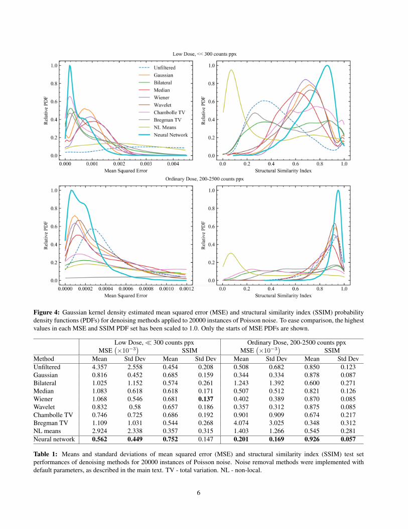
Figure 4: Gaussian kernel density estimated mean squared error (MSE) and structural similarity index (SSIM) probabilitydensity functions (PDFs) for denoising methods applied to 20000 instances of Poisson noise. To ease comparison, the highestvalues in each MSE and SSIM PDF set has been scaled to 1.0. Only the starts of MSE PDFs are shown.
Low Dose, � 300 counts ppx Ordinary Dose, 200-2500 counts ppxMSE
(×10−3
)SSIM MSE
(×10−3
)SSIM
Method Mean Std Dev Mean Std Dev Mean Std Dev Mean Std DevUnfiltered 4.357 2.558 0.454 0.208 0.508 0.682 0.850 0.123Gaussian 0.816 0.452 0.685 0.159 0.344 0.334 0.878 0.087Bilateral 1.025 1.152 0.574 0.261 1.243 1.392 0.600 0.271Median 1.083 0.618 0.618 0.171 0.507 0.512 0.821 0.126Wiener 1.068 0.546 0.681 0.137 0.402 0.389 0.870 0.085Wavelet 0.832 0.58 0.657 0.186 0.357 0.312 0.875 0.085Chambolle TV 0.746 0.725 0.686 0.192 0.901 0.909 0.674 0.217Bregman TV 1.109 1.031 0.544 0.268 4.074 3.025 0.348 0.312NL means 2.924 2.338 0.357 0.315 1.403 1.266 0.545 0.281Neural network 0.562 0.449 0.752 0.147 0.201 0.169 0.926 0.057
Table 1: Means and standard deviations of mean squared error (MSE) and structural similarity index (SSIM) test setperformances of denoising methods for 20000 instances of Poisson noise. Noise removal methods were implemented withdefault parameters, as described in the main text. TV - total variation. NL - non-local.
6

Figure 5: Mean absolute errors of our low and ordinary dose networks’ 512×512 outputs for 20000 instances of Poissonnoise. Contrast limited adaptive histogram equalization[73] has been used to massively increase contrast, revealing grid-likeerror variation. Subplots show the top-left 16×16 pixels’ mean absolute errors unadjusted. Variations are small and errorsare close to the minimum everywhere, except at the edges where they are higher. Low dose errors are in [0.0169, 0.0320];ordinary dose errors are in [0.0098, 0.0272].
4.2 Network Error
Mean absolute errors for each pixel of our network’s outputare shown for low and ordinary doses in fig. 5. Theerrors are uniform almost everywhere, except at the edgeswhere they are higher. For low and ordinary doses, themean absolute errors per pixel are 0.0177 and 0.0102,respectively.
Small, grid-like variations in absolute error are revealedby contrasted limited adaptive histogram equalization[73]in fig. 5. These variations are common in deep learningand are often associated with transpositional convolutions.Consequently, some authors[74] have recommended theirreplacement with bilinear upsampling then convolution. Wetried this; however, it only made the errors less grid-like.
Instead, we found batch normalization to be the best wayto reduce structured error variation. This is demonstratedby errors being more grid-like for the ordinary doseversion of our network, which was trained for longerafter batch normalization was frozen. Consequently, batchnormalization was not frozen until the instability introducedby its trainable variables noticeably limited convergence.
4.3 Example Usage
We provide several example applications of our low-dosenetwork to 512×512 crops from high-quality electronmicrographs that we applied noise to in fig 6 and fig. 7.Several example applications of our low-dose networkto 512×512 crops from scanning transmission electronmicrography (STEM) images are also presented in fig. 8.Our network has not been trained for STEM so thisdemonstrates its ability to generalize to other domains.
Our neural network is designed to be simple and easyto use. An example of our network being loaded once andused for inference multiple times in python is
>>> from d e n o i s e r i m p o r t D e n o i s e r>>> n o i s e r e m o v e r = D e n o i s e r ( )>>> r e s t o r e d i m g 1 = n o i s e r e m o v e r . d e n o i s e ( img1 )>>> r e s t o r e d i m g 2 = n o i s e r e m o v e r . d e n o i s e ( img2 )
Under the hood, our program divides images larger than512×512 into slightly overlapping 512×512 crops that canbe processed by our network. This gives higher accuracythan using non-overlapping crops as our network has muchhigher errors for the couple of pixels near the edges of itsoutputs. Reflection padding is applied to images beforecropping to reduce errors at their edges after restoration.Users can customize the amount overlap, padding and many
7

Noisy Restored Ground Truth
Figure 6: Example applications of the noise-removal network to instances of Poisson noise applied to 512×512 crops fromhigh-quality micrographs. Enlarged 64×64 regions from the top left of each crop are shown to ease comparison.
8

Figure 7: More example applications of the noise-removal network to instances of Poisson noise applied to 512×512 cropsfrom high-quality micrographs. Enlarged 64×64 regions from the top left of each crop are shown to ease comparison.
9

Original Denoised Original Denoised
Figure 8: Example applications of our neural network to 512×512 crops from scanning transmission electron micrographs.Enlarged 64×64 regions from the top left of each crop are shown to ease comparison. Our network has not been trained forthis domain.
10

0 5 10 15 20 25 30Batches ×103
2.5
2.0
1.5
1.0
Log 1
0(M
SE)
1 = 0.2
1 = 0.9
1 = 0.2, Batch Renorm
1 = 0.9, Batch Renorm
1 = 0.2, ReLU6
Figure 9: Batch size 2 mean squared error (MSE) learningcurves for various training hyperparameters and activationfunctions. Training is most stable for ADAM[54] β1 = 0.2without batch renormalization[75] and with ReLU6[51];rather than ReLU[76], activation.
other options or use default values we have chosen.We speed-tested our network by applying it to 20000
512×512 images with 1 external GTX 1080 Ti GPU and1 thread of a i7-6700 processor. It has a mean batch size 1(worst case) inference time of 77.0 ms. It also takes a fewseconds to load before it is ready for repeated use.
5 Additional Experiments
As part of development, we experimented with multiplearchitectures and their learning policies. Initially, weexperimented with shallower architectures similar to [18,20] and [21]; however, these struggled to meet Chambolle’slow-dose benchmark in table 1. Consequently, we switchedto the deeper Xception-based architecture presented in thispaper. In this section we present some of the experimentswe performed to fine-tune it.
5.1 Batch Size 2
Initial experiments with a batch size of 2 are summarizedin fig. 9. This includes experiments with different decayrates for the 1st moment of the momentum, β1, usedby the ADAM solver. Our results show that trainingconverges faster and more stably for β1 = 0.2 than therecommended[31, 54] β1 = 0.9. β1 = 0.9 being toohigh seems to be a theme in high resolution, low batch sizeapplications e.g. [79].
Our batch size 2 experiments also revealed that trainingis faster and more stable with ReLU6[51] than with
0 20 40 60 80 100 120Batches ×103
3.25
3.00
2.75
2.50
2.25
2.00
1.75
1.50
Log 1
0(M
SE)
Clipping, No SSIM - TrainClipping, No SSIM - ValNo Clipping, SSIM - TrainNo Clipping, SSIM - ValNo Clipping, 2.5 SSIM - TrainNo Clipping, 2.5 SSIM - ValNo Clipping, RMSProp, No SSIM - TrainNo Clipping, RMSProp, No SSIM - Val
Figure 10: Batch size 10 mean squared error (MSE)learning curves for training with and without clipping, extrastructural similarity index[77] (SSIM) based losses andRMSProp[78] rather than ADAM [54] optimization.
ReLU[76] activation. We think this is because ReLU6 isespecially effective in the decoder where it does not allowsparse activations to grow unbounded. Only ReLU-basedactivation functions were considered as the non-saturationof their gradients accelerates the convergence of stochasticgradient descent[80].
Batch renormalization[75] was trailed as our limitedhardware made large batch sizes prohibitive. We alsowanted to test how well it would work with batch size2 as we were unable to find quantitative information forthis batch size. It is ineffective: Fig. 9 shows that theextra trainable variables it introduces destabilize trainingand reduce convergence. This is not surprising as it is notdesigned for batches this small and can take time to becomeeffective. Additionally, instability introduced by applyingdifferent amounts noise to training examples may be addingto the inherent batch renormalization instability, making itmuch worse than it might be for other optimizations.
5.2 Batch Size 10
We tried adding multiples of the distance from themaximum SSIM, 1.0−SSIM, to the training loss to optimizeour network for an additional metric. As shown by fig. 10,adding different multiples does not have a significant effecton the rate of MSE convergence. Regardless, we decidedagainst adding this loss as SSIMs are weighted to measurea human perception of quality and we did not want tointroduce this slight bias. Nevertheless, we have shownthat additionally optimizing the SSIM does not significantlyaffect training.
11

Outputs were clipped between 0.0 and 1.0 beforecalculating training losses in all of our batch size 2 andthe first of our batch size 10 experiments shown in fig. 10.Removing this clipping significantly decreases the rate ofconvergence. Nonetheless, we decided to remove clippingas the network was especially prone to producing artifactsclose to 0.0 and 1.0. This ensured that these artifacts werenot present in the fully trained network’s outputs.
Following the success of lower β1 with the ADAMoptimizer, we tried other momentum-based optimizers. Thestart of a learning curve for simple RMSProp[78] is shownin fig. 10. It shows that training is significantly less stableand has a lower rate of convergence. We also experimentedwith Nesterov-accelerated gradient descent[81, 82] withsimilar results.
6 Summary
• We have developed a deep neural network for electronmicrograph denoising and shown that it outperformsexisting methods for low and ordinary electron doses.
• Fully trained versions of our network have been madeavailable for low and ordinary doses with exampleusage: https://github.com/Jeffrey-Ede/Electron-Micrograph-Denoiser
• A new dataset of 17267 2048×2048 high-qualitymicrographs collected to train our network has beenmade publicly available.
• Example applications of our network to noisy electronmicrographs are presented. We also present exampleapplication to STEM images to show that our networkcan generalize to other domains.
• Our network architecture, training hyperparametersand learning protocols are detailed. In addition, detailsof several of our initial architecture and learning policyexperiments are presented.
References
[1] E. Oho, N. Ichise, W. H. Martin, and K.-R. Peters,“Practical method for noise removal in scanningelectron microscopy,” Scanning, vol. 18, no. 1,pp. 50–54, 1996.
[2] S. J. Pennycook, “The impact of stem aberrationcorrection on materials science,” Ultramicroscopy,vol. 180, pp. 22–33, 2017.
[3] M. Linck, P. Hartel, S. Uhlemann, F. Kahl, H. Muller,J. Zach, M. Haider, M. Niestadt, M. Bischoff,J. Biskupek, et al., “Chromatic aberration correction
for atomic resolution tem imaging from 20 to 80 kv,”Physical review letters, vol. 117, no. 7, p. 076101,2016.
[4] F. Houdellier, L. De Knoop, C. Gatel, A. Masseboeuf,S. Mamishin, Y. Taniguchi, M. Delmas,M. Monthioux, M. Hytch, and E. Snoeck,“Development of tem and sem high brightnesselectron guns using cold-field emission from a carbonnanotip,” Ultramicroscopy, vol. 151, pp. 107–115,2015.
[5] T. Akashi, Y. Takahashi, T. Tanigaki, T. Shimakura,T. Kawasaki, T. Furutsu, H. Shinada, H. Muller,M. Haider, N. Osakabe, et al., “Aberration corrected1.2-mv cold field-emission transmission electronmicroscope with a sub-50-pm resolution,” AppliedPhysics Letters, vol. 106, no. 7, p. 074101, 2015.
[6] H. Adaniya, M. Cheung, C. Cassidy, M. Yamashita,and T. Shintake, “Development of a sem-basedlow-energy in-line electron holography microscopefor individual particle imaging,” Ultramicroscopy,vol. 188, pp. 31–40, 2018.
[7] C. T. Koch, “Towards full-resolution inline electronholography,” Micron, vol. 63, pp. 69–75, 2014.
[8] A. Feist, N. Bach, N. R. da Silva, T. Danz,M. Moller, K. E. Priebe, T. Domrose, J. G.Gatzmann, S. Rost, J. Schauss, et al., “Ultrafasttransmission electron microscopy using a laser-drivenfield emitter: Femtosecond resolution with a highcoherence electron beam,” Ultramicroscopy, vol. 176,pp. 63–73, 2017.
[9] V. Migunov, H. Ryll, X. Zhuge, M. Simson,L. Struder, K. J. Batenburg, L. Houben, andR. E. Dunin-Borkowski, “Rapid low dose electrontomography using a direct electron detection camera,”Scientific reports, vol. 5, p. 14516, 2015.
[10] Y. Jiang, Z. Chen, Y. Han, P. Deb, H. Gao, S. Xie,P. Purohit, M. W. Tate, J. Park, S. M. Gruner,et al., “Electron ptychography of 2d materials to deepsub-angstrom resolution,” Nature, vol. 559, no. 7714,p. 343, 2018.
[11] J. Hattne, D. Shi, C. Glynn, C.-T. Zee,M. Gallagher-Jones, M. W. Martynowycz, J. A.Rodriguez, and T. Gonen, “Analysis of global andsite-specific radiation damage in cryo-em,” Structure,2018.
[12] M. C. Motwani, M. C. Gadiya, R. C. Motwani, andF. C. Harris, “Survey of image denoising techniques,”in Proceedings of GSPX, pp. 27–30, 2004.
12

[13] Q. Zhang and C. L. Bajaj, “Cryo-electron microscopydata denoising based on the generalized digitizedtotal variation method,” Far east journal of appliedmathematics, vol. 45, no. 2, p. 83, 2010.
[14] H. S. Kushwaha, S. Tanwar, K. Rathore, andS. Srivastava, “De-noising filters for tem (transmissionelectron microscopy) image of nanomaterials,” inAdvanced Computing & Communication Technologies(ACCT), 2012 Second International Conference on,pp. 276–281, IEEE, 2012.
[15] K. Hornik, M. Stinchcombe, and H. White,“Multilayer feedforward networks are universalapproximators,” Neural networks, vol. 2, no. 5,pp. 359–366, 1989.
[16] H. W. Lin, M. Tegmark, and D. Rolnick, “Why doesdeep and cheap learning work so well?,” Journal ofStatistical Physics, vol. 168, no. 6, pp. 1223–1247,2017.
[17] Y. Bengio, A. Courville, and P. Vincent,“Representation learning: A review and newperspectives,” IEEE transactions on patternanalysis and machine intelligence, vol. 35, no. 8,pp. 1798–1828, 2013.
[18] X. Yang, V. De Andrade, W. Scullin, E. L. Dyer,N. Kasthuri, F. De Carlo, and D. Gursoy, “Low-dosex-ray tomography through a deep convolutional neuralnetwork,” Scientific reports, vol. 8, no. 1, p. 2575,2018.
[19] T. Remez, O. Litany, R. Giryes, and A. M. Bronstein,“Deep convolutional denoising of low-light images,”arXiv preprint arXiv:1701.01687, 2017.
[20] X.-J. Mao, C. Shen, and Y.-B. Yang, “Imagerestoration using convolutional auto-encoderswith symmetric skip connections,” arXiv preprintarXiv:1606.08921, 2016.
[21] K. Zhang, W. Zuo, Y. Chen, D. Meng, and L. Zhang,“Beyond a gaussian denoiser: Residual learning ofdeep cnn for image denoising,” IEEE Transactionson Image Processing, vol. 26, no. 7, pp. 3142–3155,2017.
[22] W. Xu and J. M. LeBeau, “A deep convolutional neuralnetwork to analyze position averaged convergentbeam electron diffraction patterns,” arXiv preprintarXiv:1708.00855, 2017.
[23] K. Lee, J. Zung, P. Li, V. Jain, and H. S. Seung,“Superhuman accuracy on the snemi3d connectomicschallenge,” arXiv preprint arXiv:1706.00120, 2017.
[24] D. Ciresan, A. Giusti, L. M. Gambardella, andJ. Schmidhuber, “Deep neural networks segmentneuronal membranes in electron microscopy images,”in Advances in neural information processing systems,pp. 2843–2851, 2012.
[25] Y. Zhu, Q. Ouyang, and Y. Mao, “A deepconvolutional neural network approach tosingle-particle recognition in cryo-electronmicroscopy,” BMC bioinformatics, vol. 18, no. 1,p. 348, 2017.
[26] J. Schmidhuber, “Deep learning in neural networks:An overview,” Neural networks, vol. 61, pp. 85–117,2015.
[27] S. Chetlur, C. Woolley, P. Vandermersch, J. Cohen,J. Tran, B. Catanzaro, and E. Shelhamer, “cudnn:Efficient primitives for deep learning,” arXiv preprintarXiv:1410.0759, 2014.
[28] W. Liu, Z. Wang, X. Liu, N. Zeng, Y. Liu, andF. E. Alsaadi, “A survey of deep neural networkarchitectures and their applications,” Neurocomputing,vol. 234, pp. 11–26, 2017.
[29] M. T. McCann, K. H. Jin, and M. Unser, “A review ofconvolutional neural networks for inverse problems inimaging,” arXiv preprint arXiv:1710.04011, 2017.
[30] J. Chen, X. Pan, R. Monga, S. Bengio, andR. Jozefowicz, “Revisiting distributed synchronoussgd,” arXiv preprint arXiv:1604.00981, 2016.
[31] M. Abadi, P. Barham, J. Chen, Z. Chen, A. Davis,J. Dean, M. Devin, S. Ghemawat, G. Irving, M. Isard,et al., “Tensorflow: A system for large-scale machinelearning.,” in OSDI, vol. 16, pp. 265–283, 2016.
[32] E. M. Christiansen, S. J. Yang, D. M. Ando,A. Javaherian, G. Skibinski, S. Lipnick, E. Mount,A. ONeil, K. Shah, A. K. Lee, et al., “In silicolabeling: Predicting fluorescent labels in unlabeledimages,” Cell, vol. 173, no. 3, pp. 792–803, 2018.
[33] K. He, X. Zhang, S. Ren, and J. Sun, “Delving deepinto rectifiers: Surpassing human-level performanceon imagenet classification,” in Proceedings of theIEEE international conference on computer vision,pp. 1026–1034, 2015.
[34] V. Mnih, K. Kavukcuoglu, D. Silver, A. Graves,I. Antonoglou, D. Wierstra, and M. Riedmiller,“Playing atari with deep reinforcement learning,”arXiv preprint arXiv:1312.5602, 2013.
13

[35] G. Lample and D. S. Chaplot, “Playing fpsgames with deep reinforcement learning.,” in AAAI,pp. 2140–2146, 2017.
[36] V. Firoiu, W. F. Whitney, and J. B. Tenenbaum,“Beating the world’s best at super smash bros.with deep reinforcement learning,” arXiv preprintarXiv:1702.06230, 2017.
[37] W. Xiong, J. Droppo, X. Huang, F. Seide, M. Seltzer,A. Stolcke, D. Yu, and G. Zweig, “Achieving humanparity in conversational speech recognition,” arXivpreprint arXiv:1610.05256, 2016.
[38] C. Weng, D. Yu, M. L. Seltzer, and J. Droppo,“Single-channel mixed speech recognition usingdeep neural networks,” in Acoustics, Speech andSignal Processing (ICASSP), 2014 IEEE InternationalConference on, pp. 5632–5636, IEEE, 2014.
[39] A. Santoro, D. Raposo, D. G. Barrett, M. Malinowski,R. Pascanu, P. Battaglia, and T. Lillicrap, “A simpleneural network module for relational reasoning,” inAdvances in neural information processing systems,pp. 4974–4983, 2017.
[40] Y. Wang and M. Kosinski, “Deep neural networksare more accurate than humans at detectingsexual orientation from facial images.,” Journalof personality and social psychology, vol. 114, no. 2,p. 246, 2018.
[41] Q. Yu, Y. Yang, F. Liu, Y.-Z. Song, T. Xiang, andT. M. Hospedales, “Sketch-a-net: A deep neuralnetwork that beats humans,” International Journal ofComputer Vision, vol. 122, no. 3, pp. 411–425, 2017.
[42] S. S. Han, G. H. Park, W. Lim, M. S. Kim,J. Im Na, I. Park, and S. E. Chang, “Deep neuralnetworks show an equivalent and often superiorperformance to dermatologists in onychomycosisdiagnosis: Automatic construction of onychomycosisdatasets by region-based convolutional deep neuralnetwork,” PloS one, vol. 13, no. 1, p. e0191493, 2018.
[43] T. Weyand, I. Kostrikov, and J. Philbin, “Planet-photogeolocation with convolutional neural networks,” inEuropean Conference on Computer Vision, pp. 37–55,Springer, 2016.
[44] Q. Yang, P. Yan, Y. Zhang, H. Yu, Y. Shi, X. Mou,M. K. Kalra, Y. Zhang, L. Sun, and G. Wang, “Lowdose ct image denoising using a generative adversarialnetwork with wasserstein distance and perceptualloss,” IEEE Transactions on Medical Imaging, 2018.
[45] F. Chollet, “Xception: Deep learning with depthwiseseparable convolutions,” arXiv preprint, 2016.
[46] L.-C. Chen, G. Papandreou, F. Schroff, and H. Adam,“Rethinking atrous convolution for semantic imagesegmentation,” arXiv preprint arXiv:1706.05587,2017.
[47] L.-C. Chen, Y. Zhu, G. Papandreou, F. Schroff, andH. Adam, “Encoder-decoder with atrous separableconvolution for semantic image segmentation,” arXivpreprint arXiv:1802.02611, 2018.
[48] V. Badrinarayanan, A. Kendall, and R. Cipolla,“Segnet: A deep convolutional encoder-decoderarchitecture for image segmentation,” IEEEtransactions on pattern analysis and machineintelligence, vol. 39, no. 12, pp. 2481–2495, 2017.
[49] V. Dumoulin and F. Visin, “A guide to convolutionarithmetic for deep learning,” arXiv preprintarXiv:1603.07285, 2016.
[50] S. Ioffe and C. Szegedy, “Batch normalization:Accelerating deep network training by reducinginternal covariate shift,” arXiv preprintarXiv:1502.03167, 2015.
[51] A. Krizhevsky and G. Hinton, “Convolutional deepbelief networks on cifar-10,” Unpublished manuscript,vol. 40, p. 7, 2010.
[52] A. G. Howard, M. Zhu, B. Chen, D. Kalenichenko,W. Wang, T. Weyand, M. Andreetto, and H. Adam,“Mobilenets: Efficient convolutional neural networksfor mobile vision applications,” arXiv preprintarXiv:1704.04861, 2017.
[53] K. He, X. Zhang, S. Ren, and J. Sun, “Deep residuallearning for image recognition,” in Proceedings ofthe IEEE conference on computer vision and patternrecognition, pp. 770–778, 2016.
[54] D. P. Kingma and J. Ba, “Adam: A methodfor stochastic optimization,” arXiv preprintarXiv:1412.6980, 2014.
[55] A. D. Association et al., “Tiff revision 6.0,”Internet publication: http://www. adobe.com/Support/TechNotes. html, 1992.
[56] P. J. Huber, “Robust estimation of a locationparameter,” The annals of mathematical statistics,pp. 73–101, 1964.
[57] J. Kukacka, V. Golkov, and D. Cremers,“Regularization for deep learning: A taxonomy,”arXiv preprint arXiv:1710.10686, 2017.
14

[58] T. Salimans and D. P. Kingma, “Weight normalization:A simple reparameterization to accelerate trainingof deep neural networks,” in Advances in NeuralInformation Processing Systems, pp. 901–909, 2016.
[59] X. Glorot and Y. Bengio, “Understanding the difficultyof training deep feedforward neural networks,” inProceedings of the thirteenth international conferenceon artificial intelligence and statistics, pp. 249–256,2010.
[60] G. Bradski, “The OpenCV Library,” Dr. Dobb’sJournal of Software Tools, 2000.
[61] C. Tomasi and R. Manduchi, “Bilateral filteringfor gray and color images,” in Computer Vision,1998. Sixth International Conference on, pp. 839–846,IEEE, 1998.
[62] E. Jones, T. Oliphant, P. Peterson, et al., “SciPy: Opensource scientific tools for Python,” 2001–. [Online;accessed ¡today¿].
[63] S. Van der Walt, J. L. Schonberger, J. Nunez-Iglesias,F. Boulogne, J. D. Warner, N. Yager, E. Gouillart, andT. Yu, “scikit-image: image processing in python,”PeerJ, vol. 2, p. e453, 2014.
[64] S. G. Chang, B. Yu, and M. Vetterli, “Adaptive waveletthresholding for image denoising and compression,”IEEE transactions on image processing, vol. 9, no. 9,pp. 1532–1546, 2000.
[65] D. L. Donoho and J. M. Johnstone, “Ideal spatialadaptation by wavelet shrinkage,” biometrika, vol. 81,no. 3, pp. 425–455, 1994.
[66] A. Chambolle, “An algorithm for total variationminimization and applications,” Journal ofMathematical imaging and vision, vol. 20, no. 1-2,pp. 89–97, 2004.
[67] T. Goldstein and S. Osher, “The split bregmanmethod for l1-regularized problems,” SIAM journal onimaging sciences, vol. 2, no. 2, pp. 323–343, 2009.
[68] P. Getreuer, “Rudin-osher-fatemi total variationdenoising using split bregman,” Image Processing OnLine, vol. 2, pp. 74–95, 2012.
[69] A. Buades, B. Coll, and J.-m. Morel, “Jm: A non-localalgorithm for image denoising,” in In: ComputerVision and Pattern Recognition, 2005. CVPR 2005.IEEE Computer Society Conference on, Citeseer,2005.
[70] B. A. Turlach, “Bandwidth selection in kernel densityestimation: A review,” in CORE and Institut deStatistique, Citeseer, 1993.
[71] D. M. Bashtannyk and R. J. Hyndman, “Bandwidthselection for kernel conditional density estimation,”Computational Statistics & Data Analysis, vol. 36,no. 3, pp. 279–298, 2001.
[72] D. W. Scott, Multivariate density estimation: theory,practice, and visualization. John Wiley & Sons, 2015.
[73] K. Zuiderveld, “Contrast limited adaptive histogramequalization,” Graphics gems, pp. 474–485, 1994.
[74] A. Odena, V. Dumoulin, and C. Olah, “Deconvolutionand checkerboard artifacts,” Distill, vol. 1, no. 10,p. e3, 2016.
[75] S. Ioffe, “Batch renormalization: Towards reducingminibatch dependence in batch-normalized models,”in Advances in Neural Information ProcessingSystems, pp. 1942–1950, 2017.
[76] V. Nair and G. E. Hinton, “Rectified linearunits improve restricted boltzmann machines,” inProceedings of the 27th international conference onmachine learning (ICML-10), pp. 807–814, 2010.
[77] Z. Wang, A. C. Bovik, H. R. Sheikh, and E. P.Simoncelli, “Image quality assessment: from errorvisibility to structural similarity,” IEEE transactionson image processing, vol. 13, no. 4, pp. 600–612,2004.
[78] G. Hinton, N. Srivastava, and K. Swersky, “Neuralnetworks for machine learning lecture 6a overview ofmini-batch gradient descent,” Cited on, p. 14, 2012.
[79] T.-C. Wang, M.-Y. Liu, J.-Y. Zhu, A. Tao, J. Kautz,and B. Catanzaro, “High-resolution image synthesisand semantic manipulation with conditional gans,”arXiv preprint arXiv:1711.11585, 2017.
[80] A. Krizhevsky, I. Sutskever, and G. E. Hinton,“Imagenet classification with deep convolutionalneural networks,” in Advances in neural informationprocessing systems, pp. 1097–1105, 2012.
[81] I. Sutskever, J. Martens, G. Dahl, and G. Hinton,“On the importance of initialization and momentumin deep learning,” in International conference onmachine learning, pp. 1139–1147, 2013.
[82] Y. Nesterov, “A method of solving a convexprogramming problem with convergence rate o(1/k2),” in Soviet Mathematics Doklady, vol. 27,pp. 372–376, 1983.
15