JCOMM TR No. 84 - Seawater Salinity Intercomparison Pilor …€¦ · Web view · 2016-11-29Final Report, JCOMM Pilot Intercomparison Project for Seawater Salinity Measurements

World MeteorologicalOrganization

WORLD METEOROLOGICAL ORGANIZATION

_____________

INTERGOVERNMENTAL OCEANOGRAPHIC COMMISSION (OF

UNESCO)_____________

FINAL REPORT, JCOMM PILOT INTERCOMPARISON PROJECT FOR SEAWATER

SALINITY MEASUREMENTS

2015

JCOMM Technical Report No. 84


[page left intentionally blank]

- 2 -

JCOMM Technical Report No. 84WORLD METEOROLOGICAL ORGANIZATION

_____________

INTERGOVERNMENTAL OCEANOGRAPHIC COMMISSION (OF UNESCO)

___________

Final Report, JCOMM Pilot Intercomparison Project forSeawater Salinity Measurements

2015


- 3 -


NOTES

WMO DISCLAIMER

Regulation 42

Recommendations of working groups shall have no status within the Organization until they have been approved by the responsible constituent body. In the case of joint working groups the recommendations must be concurred with by the presidents of the constituent bodies concerned before being submitted to the designated constituent body.

Regulation 43

In the case of a recommendation made by a working group between sessions of the responsible constituent body, either in a session of a working group or by correspondence, the president of the body may, as an exceptional measure, approve the recommendation on behalf of the constituent body when the matter is, in his opinion, urgent, and does not appear to imply new obligations for Members. He may then submit this recommendation for adoption by the Executive Council or to the President of the Organization for action in accordance with Regulation 9(5).

© World Meteorological Organization, 2023

The right of publication in print, electronic and any other form and in any language is reserved by WMO. Short extracts from WMO publications may be reproduced without authorization provided that the complete source is clearly indicated. Editorial correspondence and requests to publish, reproduce or translate this publication (articles) in part or in whole should be addressed to:

Chairperson, Publications BoardWorld Meteorological Organization (WMO)7 bis, avenue de la Paix Tel.: +41 (0)22 730 84 03P.O. Box No. 2300 Fax: +41 (0)22 730 80 40CH-1211 Geneva 2, Switzerland E-mail: [email protected]

IOC (OF UNESCO) DISCLAIMER

The designations employed and the presentation of material in this publication do not imply the expression of any opinion whatsoever on the part of the Secretariats of UNESCO and IOC concerning the legal status of any country or territory, or its authorities, or concerning the delimitation of the frontiers of any country or territory.

____________

- 4 -


C O N T E N T S

1． Preface2． Project Introduction...............................................................................................2.1 Start2.2 Project Implementation Outline（See Annex A）2.3 Project Design3． Results and Discussion3.1 Group α3.2 Group β3.3 Additional Information4． Technical Analysis and Discussion4.1 Measuring Instruments4.2 Linearity Correction4.3 SSW for Standardization4.4 Measurement Uncertainty4.5 Drift of SSW Salinity Value5． Summary6． Acknowledgment7． References

Annex A Project Organization and Implementation ...........................................................20Annex B Organizing Committee and Working Group membership ....................................22Annex C Seawater Sample Introduction ............................................................................23Annex D Operation Guideline.............................................................................................30Annex E Introduction of Measuring Instruments Used in the Project..................................35Annex F Example for Uncertainty Evaluation of Salinity Measurement Result .................41Annex G Acronyms.............................................................................................................44

_____________

- 5 -



- 6 -


FINAL REPORT, JCOMM PILOT INTERCOMPARISON PROJECT FOR SEAWATERSALINITY MEASUREMENTS

1．Preface

The Pilot Inter-comparison Project for Seawater Salinity Measurements is organized by The Joint WMO-IOC Technical Commission for Oceanography and Marine Meteorology (JCOMM) and undertaken by the Regional Marine Instrument Center for the Asia-Pacific Region (RMIC/AP). As the first inter-comparison project under JCOMM framework in history, the purpose is of understanding the overall quality level of salinity measurements of JCOMM Members/Member States and observation programmes, identifying the differences and promoting the expertise of salinity measurements.

Salinity is one of the basic parameters acknowledged in the oceanography community, and has important significance for oceanographic research and many industries. International programmes under or related to JCOMM, such as the Data Buoy Cooperation Panel (DBCP), the Ship Observations Team (SOT), the Global Sea-Level Observing System (GLOSS), the Argo profiling float programme, the Ocean Sustained Interdisciplinary Timeseries Environment observation System (OceanSITES), the International Ocean Carbon Coordination Project of IOC (IOCCP), or the Global Ocean Ship-Based Hydrographic Investigations Programme (GO-SHIP), carry out seawater salinity measurements. At present, comparing the salinity data of natural seawater measured in the laboratory with the corresponding data in situ measurements is deemed as a quality control method, the accuracy of which is essential to the data quality of JCOMM marine observational programmes. Therefore, it is indispensable to implement this project.

The inter-comparison project was designed and implemented with respect to ISO/IEC 17043:2010 Conformity Assessment General Requirements for Proficiency Testing. It needs to be clarified that this project is not a Proficiency Testing and is developed without the intention to evaluate the participants’ capabilities of salinity measurement. It is also not recommended that any organization should take this report as a reference to evaluate the participating laboratories on their measurement capabilities; for confidence, the participants will carry anonymous ID codes in this report. Meanwhile, during this inter-comparison, participants have made good measurements of well-prepared samples under good conditions, so it is not certain to be an indicator of the quality of salinity measurements with samples collected and analyzed in ordinary fieldwork situations. As an inter-comparison activity, differences are definitely seen among the participants. We hope that through comparison and deeper analysis of these differences, actual technical issues related to salinity measurement in the laboratory would be touched, which in turn may help to improve salinity measurement quality level.

This report will introduce in detail the organization, implementation and data analysis of this activity, where results of all participating laboratories and charts are included.

2．Project Introduction

2.1 Start

During the 5th session of the JCOMM Observations Coordination Group (OCG, September 2013, Silver Spring, Maryland, USA), the Chief Director of the Regional Marine Instrument Center for Asia Pacific, namely NCOSM (National Center of Ocean Standard and Metrology, China), proposed to develop a project on inter-comparison of seawater salinity measurement with the purpose of supporting the JCOMM observational program. NCOSM was willing to undertake the project and submitted the proposal which was eventually approved by the conference.

- 7 -


In January 2014, the OCG Chair and the JCOMM co-Presidents approved the Terms of Reference (ToR) and the membership of the Organizing Committee (OC, see Annex B). On the basis of proposal on OCG-5, the OC submitted the formal international comparison working documents in February 2014 and received approval from the OCG Chair and JCOMM co-Presidents. Meanwhile, the JCOMM co-Presidents formally authorized RMIC/AP to undertake this activity which was appointed as a JCOMM pilot project.

2.2 Project Implementation Outline （See Annex A）

In December 2013, the OC and its ToR were set up. The OC drafted the working plan and the Operation Guideline.

On December 25th 2013, a Working Group (WG) was established in RMIC/AP (See Annex B for the membership).

From March to May 2014, the OC sent formal invitations to WMO & IOC member states and started to accept registration.

In May 2014, RMIC/AP prepared two batches of seawater samples (Sample A & Sample B), 300 bottles for each batch according to the Implementation Scheme.

In July 2014, RMIC/AP delivered the samples to all participants. Addition samples were delivered to two participants in May and November respectively.

From July to August 2014, the participating laboratories received the samples, took measurements and submitted results. RMIC/AP drafted a Periodical Summary and submitted it to the OC.

In September 2014, RMIC/AP collected data for analysis and kept contact with the laboratories on technical problems.

From October to November 2014, RMIC/AP drafted a Final Report and kept contact with the laboratories.

In December 2014, the Final Report was completed and submitted to the OC for further scrutiny and remarks, and approval.

2.3 Project Design

The design of the inter-comparison project refers to the ISO/IEC 17043:2010 Conformity assessment General Requirements for proficiency testing. The inter-comparison project is not a proficiency testing, so not every item in ISO/IEC 17043 is applicable to the project.

2.3.1 Sample (See Annex C)

Seawater samples of two different salinity values (30~35, 20~25), labeled with SAMPLE A and SAMPLE B respectively, are provided. In this report, the term “salinity” means Practical Salinity on the scale of 1978 (PSS-78). The project requires participating laboratories to measure these two seawater samples according to the Operation Guideline and to report the result.

RMIC/AP prepared the seawater samples and was responsible for their homogeneity and stability. The samples were packaged with waterproof carton and the gaps were filled with cushion material before shipped to each participating laboratory via express shipment. Operation Guideline, Receipt Form, Participant ID Code and Results Sheet were shipped along with the samples.

Homogeneity and stability tests were carried out with respect to ISO GUIDE 35:2006 Reference materials - General and statistical principles for certification. Samples were taken for the homogeneity test and the stability test. Meanwhile, environmental tests such as a high/low

- 8 -


alternating temperature test were performed in order to check and guarantee the reliability of the samples.

2.3.2 Operation Guideline（See Annex D）

In order to guide the operation of the participants, documents (Operation Guideline, Receipt Form and Results Sheet) were distributed. Salinity was specified as the testing objective parameter and was recommended to be measured by means of a conductivity measurement; however, any other methods were also acceptable. Results format, decimal places of the result and the way to express uncertainty were also specified in the Results Sheet.

Submission of the original record and measurement method were required to submit for facilitating the result analysis process.

2.3.3 Statistical Method

With reference to ISO 5725-2:1994 Accuracy (trueness and precision) of measurement methods and results- Part 2: Basic method for the determination of repeatability and reproducibility of a standard measurement method, Grubbs test method was used at the very beginning to eliminate outliers within data sets. The median of the remaining data sets and the biases of the participating laboratories were calculated according to the calculation method in ISO 13528:2005 Statistical methods for use in proficiency testing by interlaboratory comparisons.

2.3.4 Confidentiality

For confidential purpose, each laboratory was represented by an assigned ID Code in the Final Report when it comes to the results and the analyses.

3．Results and Discussion

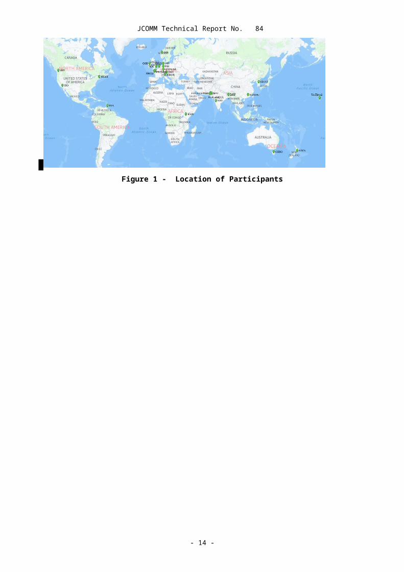
A total of 26 laboratories from 17 countries (Table 1) registered in the inter-comparison project, including universities, institutes, governmental agencies, and commercial companies. From regional perspective, the participants come from different continents including Africa, Asia, Europe, North America and Oceania.

Results were reported from 25 laboratories (except the participant from Kenya, which quitted the project), of which 20 used laboratory salinometers and 5 used hand-held measuring instruments, for statistics denoted here as the group α and the group β, respectively.

Figure 1 - Location of Participants

- 9 -


Table 1 - Participant List

Country InstitutionAustralia CSIRO Marine and Atmospheric Research (CSIRO)

Bangladesh Institute of Marine Sciences and Fisheries (IMSF)

Belgium Royal Belgian Institute of Natural Sciences-OD Nature- MARCHEM (RBINS)

China South China Sea Environmental Monitoring Center (SCSEMC)

France IFREMER Centre de Brest REM/RDT/LDCM (IFREMER)Service Hydrographique et Ocean-ographique de la Marine (SHOM)

Germany

Alfred-Wegener-Institut Helmholtz Zentrum für Polar und Meeresforschung (AWI)

Bundesamt für Seeschifffahrt und Hydrographie (BSH)GEOMAR Helmholtz Centre for Ocean Research Kiel (GEOMAR)

India National Institute of Oceanography (NIO)Ireland Ocean Science and Information Services，Marine Institute (OSIS)

ItalyIstituto Nazionale di Oceanografia e di Geofisica Sperimentale (OGS)

CNR-ISMAR Institute of Marine Science- U.O.S. Pozzuolo di Lerici (ISMAR)

KoreaKorea Institute of Ocean Science & Technology Oceanographic Measurement & Instrument Calibration Service Center (KIOST

OMICS)Kenya Kenya Meteorological Service (KMS)

New Zealand NIWA Ocean CTD Facility (NIWA)

Norway Institute of Marine Research-Oceanography and Climate Research Group (IMR)

Pakistan

Centre of Excellence in Marine Biology University of Karachi (Un. Karachi)

National Institute of Oceanography (NIO)Faculty of Marine Sciences, Lasbela University of Agriculture, Water

and Marine Sciences (FMS/LUAWMS)Trinidad & Tobago Institute of Marine Affairs (IMA)

United Kingdom National Oceanography Centre (NOC)

USA

Scripps Institution of Oceanography, Oceanographic Data Facility (SIO)

Woods Hole Oceanographic Institution (WHOI)Sea-Bird Electronics (Seabird)

Oceanography Research Associate University of Hawaii (Un. Hawaii)

- 10 -


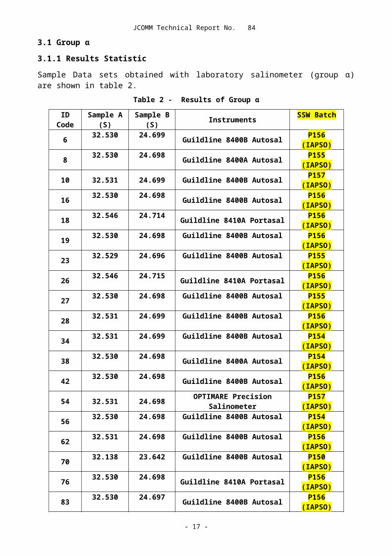
3.1 Group α

3.1.1 Results Statistic

Sample Data sets obtained with laboratory salinometer (group α) are shown in table 2.

Table 2 - Results of Group α

ID Code Sample A (S) Sample B (S) Instruments SSW Batch6 32.530 24.699 Guildline 8400B Autosal P156 (IAPSO)8 32.530 24.698 Guildline 8400A Autosal P155 (IAPSO)

10 32.531 24.699 Guildline 8400B Autosal P157 (IAPSO)16 32.530 24.698 Guildline 8400B Autosal P156 (IAPSO)18 32.546 24.714 Guildline 8410A Portasal P156 (IAPSO)19 32.530 24.698 Guildline 8400B Autosal P156 (IAPSO)23 32.529 24.696 Guildline 8400B Autosal P155 (IAPSO)26 32.546 24.715 Guildline 8410A Portasal P156 (IAPSO)27 32.530 24.698 Guildline 8400B Autosal P155 (IAPSO)28 32.531 24.699 Guildline 8400B Autosal P156 (IAPSO)34 32.531 24.699 Guildline 8400B Autosal P154 (IAPSO)38 32.530 24.698 Guildline 8400A Autosal P154 (IAPSO)42 32.530 24.698 Guildline 8400B Autosal P156 (IAPSO)54 32.531 24.698 OPTIMARE Precision Salinometer P157 (IAPSO)56 32.530 24.698 Guildline 8400B Autosal P154 (IAPSO)62 32.531 24.698 Guildline 8400B Autosal P156 (IAPSO)70 32.138 23.642 Guildline 8400B Autosal P150 (IAPSO)76 32.530 24.698 Guildline 8410A Portasal P156 (IAPSO)83 32.530 24.697 Guildline 8400B Autosal P156 (IAPSO)86 32.526 24.695 Guildline 8410A Portasal P9 (NCOSM)

Note: The salinity values of two samples measured by RMIC/AP are respectively 32.5299 (Sample A) and 24.6973 (Sample B). On the basis of data from homogeneity and stability tests (Annex C), the combined standard uncertainties of these two factors areu(Sample A)=0.0005, u(Sample B)=0.0003

After eliminating outliers by adopting the Grubbs test, the results are as follows

Table 3 - Results After Outliers Removed

ID Code Sample A (S) Sample B (S)6 32.530 24.6998 32.530 24.698

10 32.531 24.69916 32.530 24.69819 32.530 24.69823 32.529 24.69627 32.530 24.69828 32.531 24.69934 32.531 24.69938 32.530 24.69842 32.530 24.69854 32.531 24.69856 32.530 24.69862 32.531 24.69876 32.530 24.69883 32.530 24.697

- 11 -


3.1.2 Calculation of Assigned Value

The robust-average data from table 3 are used to calculate comparison reference value (CRV) X , by

X=median( X i)

for the two columns i. The CRVs of Sample A/B are shown in table 4

Table 4 - The CRVs of Sample A/B

Median Sample A (S) Sample B (S)X 32.530 24.698

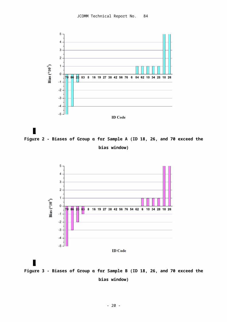
3.1.3 Bias

The following equation is used to calculate the bias,

Di=x i−X

where X is the assigned value, x is the result measured by each laboratory, and i is the ID code of participating laboratory..

Biases of 20 laboratories are shown in table 5, Fig 2 & Fig 3. Four biases are notably larger while the others are consistent.

Table 5 - Biases of Group α

ID Code Bias of Sample A(×10-3)

Bias of Sample B(×10-3)

6 0 18 0 0

10 1 116 0 018 16 1619 0 023 -1 -226 16 1727 0 028 1 134 1 138 0 042 0 054 1 056 0 062 1 070 -392 -105676 0 083 0 -186 -4 -3

- 12 -


Figure 2 - Biases of Group α for Sample A (ID 18, 26, and 70 exceed the bias window)

Figure 3 - Biases of Group α for Sample B (ID 18, 26, and 70 exceed the bias window)

3.2 Group β

Sample data sets obtained with hand-held instruments are included in group β, shown in table 6. The analysis of group β will not adopt the statistical method of group α, in light of insufficient samples, large differences and lower measuring precision within the group. So the only thing done

- 13 -


is comparing the bias with maximum permissible errors (MPE) of the instrument used. Results are shown in table 7.

Table 6 - Results of Group β

ID Code Sample A Sample B Instrument

21 31.60 24.07 YSI Professional Plus Handheld Multi-parameter

36 30.922 25.920 ELMETRON CPC401

46 33.5 25.0 ATAGO Hand-Held Refractometer S/Mill-E

57 29 21 ATAGO Hand-Held Refractometer S/Mill-E

66 32.3 24.49 YSI Professional Plus Handheld Multi-parameter

Table 7 - Biases of Group β

ID Code

Bias ofSample A

Bias ofSample B MPE of Instrument* Result

21 -0.93 -0.63 ±1.0% of reading or 0.1 ppt, whichever is greater Exceed MPE

36 -1.608 1.222 ±0.1%; > 20 mS/cm: ±0.25%（Conductivity） Exceed MPE

46 1.0 0.3 ±1‰ In the range of MPE

57 -3.5 -3.7 ±1‰ Exceed MPE

66 -0.23 -0.21 ±1.0% of reading or ±0.1 ppt, whichever is greater

In the range of MPE

Note: *Information from instrument manufacturer.

3.3 Additional Information

3.3.1 With respect to the Operation Guideline, all 25 participating laboratories returned the Result Sheet. However, some information such as environmental conditions and specification of instrument in part of these sheets was omitted. Some participants even failed to complete the standardization information. The missing information was supplemented during communication between project WG and participants.

3.3.2 Considering the resolution and the accuracy class of the common instruments and the requirements of actual applications of salinity measurements as well, participants were required, in Operation Guideline (Annex D), to submit results with 3 decimal places. However, some participants maintained 4 decimal places in their results which were rounded off later to 3 decimal places by WG when processing data.

3.3.3 Following the recommendation of the Operation Guideline, several laboratories submitted the Result Sheet together with uncertainty estimates, and a few also with data processing methods (linearity correction, Standard Seawater (SSW) drift correction), which is helpful to analyze the results.

- 14 -


4．Technical Analysis and Discussion

4.1 Measuring Instruments

Two kinds of measuring instruments were used in the inter-comparison project, namely laboratory salinometers and hand-held salinity (conductivity) instruments. 20 laboratories used laboratory salinometers and 5 laboratories used hand-held instruments, as shown in table 8.

Table 8 - Instruments Used in the Project

Group Instruments Amount

α

Guildline 8400B Autosal 13Guildline 8410A Portasal 4Guildline 8400A Autosal 2

OPTIMARE Precision Salinometer 1

β

YSI Professional Plus Handheld Multi-parameter 2

ELMETRON CPC401 1ATAGO Hand-Held Refractometer

S/Millα-E2

(i) Four models of salinometers were used in the project. Among them, 8400B & 8410A salinometers from Guildline Instruments are the most used ones, for which a stable measurement environment is necessary, otherwise the accuracy class of the instrument could not meet the requirements. Therefore, for high precision salinity measurement, laboratory salinometers should be taken and calibrated as necessary; more importantly, the measurement should be carried out under stable environmental conditions.

(ii) It is understandable that biases of group β are greater because of the instrumental accuracy constraint. However, biases from 3 laboratories exceed the MPE of corresponding instrument. Laboratories concerned should make sure that the instrument is in good condition, the measurement is performed with regard to instructions, and the instrumental calibration is still valid. RMIC/AP WG welcomes further communication from any laboratories.

See Annex E for detailed introduction of measuring instruments used in the project.

4.2 Linearity Correction

In the inter-comparison project, some laboratories reported detailed operational records along with the results, including standardization and linearity correction information. Since a lot of laboratories used the 8400B salinometer for measuring salinity, the linearity correction is discussed here.

According to the discussion in section 4.1, the 8400B should be calibrated with the International Association for the Physical Sciences of the Oceans (IAPSO) SSW series pack or equivalent. It is known from the 8400B technical manual that the instrument’s MPE is better than ±0.002 within 24hours on the salinity range of 2~38. Whether to perform a linearity correction depends on the level of measurement accuracy and two typical situations are described here below.

(i) If the measurement result meets the accuracy requirement, linearity correction could not be taken into consideration, but if this step is done, the result could be more satisfactory.

(ii) If the result failed to meet that requirement, it should be linearity-corrected. Only two salinity points are needed for linearity corrections as long as the sample seawater

- 15 -


salinity falls between these two points. The procedure is detailed below with an example in which salinity sample is 25.

Step 1: Standardize the salinometer with SSW (salinity=35);

Step 2: Measure SSW (salinity=10 and 30, respectively) and obtain the results;

Step 3: Perform a linearity regression with Y (the standard salinity value) and X (measured salinity value), and get the equation Y=a+bX;

Table 9 - Measurement Results (tutorial example)

Standard Salinity Value Y Measured Salinity Value X9.998 10.0024

30.003 30.0039

Figure 4 - Linearity Regression (tutorial example)

Step 4: Take the measured salinity result of the unknown sample into the equation and obtained the final result.

If applied or not, the linearity corrections can affect slightly the assigned value calculated in 3.1.2 and the bias calculated in 3.1.3.

4.3 SSW for Standardization

Instruments were standardized with SSW by 20 laboratories in group α among which 19 laboratories used IAPSO SSW (OSIL, UK) and 1 laboratory used Chinese SSW (NCOSM, CHINA). The RMIC/AP WG performed some experiments to analyze the potential difference caused by using different SSWs for standardization. Standardize the salinometer with IAPSO SSW, then measure Sample A and Sample B respectively (3 times and averaging); then repeat procedures above under the same conditions, except taking Chinese SSW for standardization. Results are shown in table 10 where the D-value is 0.0006 for sample A and 0.0004 for sample B. We also know that the

- 16 -


expanded uncertainty of both SSWs is U=0.001，k=2, whereupon those D-values are no greater than the square root of the sum of square (0.0014) of expanded uncertainty of those two kinds of SSW. Therefore, we believe that the usage of two kinds of SSW does not notably affect the measurement results.

Table 10 - Comparison of Results Standardized by Different SSW

SSW for Standardization Chinese SSW (S) IAPSO SSW (S)

Batch P9 P155

ResultsSample A 32.5291 32.5297Sample B 24.6973 24.6977

DifferenceSample A 0.0006Sample B 0.0004

4.4 Measurement Uncertainty

Measurement uncertainty is widely used in various measurement fields. BIPM as well as other 6 international organizations co-issued the Guide to the Expression of Uncertainty in Measurement, called GUM for short as below, which is the basis for uniformly adopting and evaluating uncertainty of measurement all over the world. The most recent GUM version is ISO/IEC Guide98-3:2008.

Participating laboratories were encouraged to give out results with uncertainty in the inter-comparison, and eventually, 9 laboratories gave out the uncertainty (see table 11), and most part of that are in the vicinity of 0.002. Through the reported uncertainty, analyst has learned the reliability of the results and understood more measurement details. Participants who take the trouble to provide an uncertainty have done a reasonable job of it.

The uncertainty evaluation of practical salinity measurements was studied earlier. Le Menn (2011) gave the procedure of uncertainty evaluation of salinity measured by salinometers with the GUM method and the Monte Carlo method. The expanded uncertainty results were 0.0016, 0.0022 and 0.0025 (0.0024), respectively, when seawater samples of 10, 35, and 40 (salinity) were measured. Bacon et al. (2007) assessed the uncertainty of the K15 value of IAPSO SSW, concluding that the expanded uncertainty of conductivity ratio is 1×10-5. Perkin and Lewis (1980) calculated the standard deviation of the PSS-78 fitting formula, the result of which was 0.0007 (salinity). Referring to the studies above, a method of uncertainty estimation for salinity seawater sample measurement is given here for reference (see Annex F).

Table 11 - Uncertainty Reported by Several Part Laboratories

ID Code Sample A Sample B Comment10 0.001 0.001 k=218 0.049 0.037 k=219 0.0026 0.0026 k=2

27 0.0002 0.0001 Repeatability Componentk=2

28 0.0005 0.0005 Repeatability Component, k=2.571

34 0.002 0.002 k=262 0.0022 0.0020 k=2

- 17 -


83 0.002 0.002 k=286 0.002 0.002 k=2

4.5 Drift of SSW Salinity Value

Some laboratories considered the drift of SSW and accordingly corrected the final result. In light of the discussion of Culkin and Ridout (1998) and Bacon et al. (2007), the SSW batches P130–P144 have zero offset. Therefore a correction for SSW drift has a very small effect on the result. Usually, it is recommended that salinometer users should ignore the drift of SSW within the validity, unless evident drift is observed. However, users who need to obtain even higher accuracy should take SSW drift into account and accordingly make a correction.

In addition, the SSW used by one participating laboratory was out of date (P150, 2008) which may have drifted significantly and likely caused the large biases. Actually, the biases of this participant are the largest of all.

5．Summary

The Pilot Inter-Comparison Project for Seawater Salinity Measurements, in which 25 laboratories from 16 countries took part, is the first ever inter-comparison project held within the JCOMM framework. Since typical laboratories around the world participated in the project, an objective understanding of the current quality level of seawater salinity measurements could be obtained. In the meantime, the project also provided an opportunity for participating laboratories to detect potential problems in their measurements and thus helped to improve the salinity measurement quality.

1) For those 20 laboratories that utilized laboratory salinometers (Group α), 16 results are relatively consistent, and the other 4 have substantial biases. Concerning that the uncertainty of SSW is of order 0.001 to 0.002, 16 of the labs made high quality measurements, largely indistinguishable from one another. Lab 86 has small errors, which may be corrected with minor adjustment to their measurement procedures. Labs 18 and 26 had larger errors, of order 0.02. This might or might not be important depending on the purpose for which they make measurements. Lab 70 clearly has significant problems, with major defect either in the equipment or operation.

2) For those 5 laboratories using hand-held instruments (Group β), due to the lower measurement accuracy compared with Group α, their biases were calculated with respect to assigned value of Group α. Finally 3 of them exceeded the corresponding instrument MPE.

Reviewing the whole inter-comparison project, several conclusions can be drawn:

1) The inter-comparison project reflected the differences of salinity measurement capabilities among participating laboratories all over the world;

2) Among several seawater salinity measurement methods, measuring with laboratory salinometers and SSW can lead to a higher measurement level and consistency;

3) During the Pilot Inter-comparison Project for Seawater Salinity Measurements, noticeable technical problems arose, and valuable experience was accumulated.

It is hoped that the results should be helpful to the global marine observational programme. It is recommended that more JCOMM inter-comparison projects should be held and have more participants involved in the future.

- 18 -


6．Acknowledgment

The sincere gratitude goes to RMIC/AP, who undertook the project, established the WG and provided full support to its work such as communicating with participants, manufacturing and delivering SSW samples, ensuring the sample quality, processing data and drafting the Final Report.

Thanks to every participating laboratory for its active involvement which is highly appreciated.

Thanks to Guildline Instruments as well for providing technical suggestions on their salinometers.

Thanks to Dr. Rainer Feistel (SCOR/IAPSO),Prof. Steffen Seitz and Prof. Richard Pawlowicz for their valuable review of this report.

7．References

Bacon, S., Culkin, F., Higgs, N., and Ridout, P.: IAPSO Standard Seawater: definition of the uncertainty in the calibration procedure and stability of recent batches, J. Atmos. Oceanic Technol., 24, 1785–1799, 2007.

BIPM: Evaluation of measurement data – Guide to the expression of uncertainty in measurement, JCGM 100:2008, GUM 1995 with minor corrections, 2008.

BIPM: Evaluation of measurement data – Supplement 1 to the Guide to the expression of uncertainty in measurement – Propagation of distributions using a Monte Carlo method, JCGM 101:2008, 2008

Culkin, F. and Ridout, P. S.: Stability of IAPSO Standard Seawater, J. Atmos. Oceanic Technol., 15, 1072–1075, 1998.

ISO/IEC 17043:2010 Conformity assessment General Requirements for proficiency testing

ISO GUIDE 35:2006 Reference materials - General and statistical principles for certification

ISO 13528:2005 Statistical methods for use in proficiency testing by interlaboratory comparisons

ISO 5725-2:1994 Accuracy (trueness and precision) of measurement methods and results- Part 2: Basic method for the determination of repeatability and reproducibility of a standard measurement method

Le Menn, M.: About uncertainties in practical salinity calculations. Ocean Sci., 7, 651-659, 2011.

Perkin, R. G. and Lewis, E. L.: The Practical Salinity Scale 1978: Fitting the Data, IEEE J. Oceanic Eng., OE-5, no. 1, 9–16, 1980.

____________

- 19 -


ANNEX A

PROJECT ORGANIZATION AND IMPLEMENTATION

1. During the 5th session of OCG (September 2013, Silver Spring, Maryland, USA), Chief Director of Regional Marine Instrument Center for Asia Pacific (RMIC/AP), namely NCOSM (National Center of Ocean Standard and Metrology, China), proposed to develop a project on inter-comparison of seawater salinity measurement in the purpose of serving JCOMM observational programme. RMIC/AP was willing to undertake the project and submitted the draft Implementation Scheme, Work Plan, Operation Guideline for discussion that had eventually been approved by the conference.

2. In December 2013, RMIC/AP established a working group (WG) responsible for the contact, implementation and technical support of the project. The WG drafted Terms of Reference (ToR) for the Organizing Committee (OC), proposed members of the OC, and consulted to WMO secretariat, IOC secretariat and oceanography experts. With support of WMO and IOC officials, a special zone was established on JCOMM website where documents as Invitation Letter were released.

3. From January to February 2014, on the basis of documents on OCG-5, the OC submitted the formal inter-comparison working documents (List of OC Members, ToR, Work Plan, Implementation Scheme, Operation Guideline and Registration Form) which were approved by OCG president and JCOMM co-president. Meanwhile, JCOMM co-president formally authorized RMIC/AP to undertake this project which was appointed to be a JCOMM pilot project. SUN Jingli (RMIC/AP) was elected as president of OC, PANG Yongchao (Director of test and calibration center, RMIC/AP) was elected as member of the OC.

4. From March to May 2014, the OC sent formal Invitations to WMO & IOC member states and started to accept registration. The OC and RMIC/AP made effective communication with participants. During this period of time, RMIC/AP actively offered information about this project to participants (countries) of the past RMIC/AP Workshop and finally increased participants number. In May, a pair of sample was delivered to a participant in advance for reason that the participant was planned on cruise for ocean investigation and could not receive samples as per the original plan.

5. From May 5th to 10th 2014, RMIC/AP manufactured two batches of seawater samples, 300 bottles each according to the Implementation Scheme. Salinity value of one batch ranges from 20 to 25 and the other from 30 to 35. Homogeneity test was performed and the results met the requirement of the inter-comparison.

6. Since June 2014, RMIC/AP performed stability test for 6 times. The result was good enough to meet requirement of the inter-comparison.

7. As of July 16th, RMIC/AP received registration of 25 laboratories from 17 countries. After fully communication and confirming the delivery address with each participant, samples (Operation Guideline included) were delivered. Before delivery, the WG designed sample label and package. The reliability and stability of the package were verified through experiments. In addition, the samples passed air transportation and classification identification and were delivered.

8. From July to August, participants confirmed to receive samples and took measurement. During this time, WG contacts participants for many times with regards to the receipt and intactness of the samples. From late July to early September, RMIC/AP received results and kept contact by

- 20 -


email with those participants who didn’t give a feedback. Among them, one participant quitted the project due to unexpected accident.

9. In September 2014, RMIC/AP collected all results from participating laboratories and started a preliminary check. For results with obvious problem or missing important information, RMIC/AP kept close contact with corresponding laboratories for further details. Specifically, result from a certain laboratory was an apparent anomaly in this case RMIC/AP decided to send again the sample for measurement and finally obtained an acceptable result. After collecting all the data, a statistical analysis was done.

10. In October 2014, RMIC/AP started to draft the Final Report and contact with laboratories with regard to technical problems in order to know the process of measurement and analyze which part could the problem come from.

11. In November 2014, the University of Hawaii took part in this activity, and their results were included in the statistical analysis.

12. In December 2014, RMIC/AP modified the draft Final Report on the basis of an internal discussion, and submitted it to the OC.

13. In January 2015, the OC reviewed the draft Final Report, and enquired several oceanography experts for their suggestions as well.

14. The Final Report was approved by the OC.

____________

- 21 -


ANNEX B

ORGANIZING COMMITTEE AND WORKING GROUP MEMBERSHIPS

B.1 Membership of the JCOMM Inter-comparison Project for Seawater Salinity Measurements

Organizing Committee

Jingli SUN (NCOSM, China), Chair, Organizing Committee

Yongchao PANG (NCOSM, China), Activity leader

Brian King (NOC, UK), Argo Steering Team & GO-SHIP

Robert Weller (WHOI, USA), Co-chair, OceanSITEs

Marc Le Menn (SHOM, France), GOSUD

Representative of the SOOP - TBD

Tom Gross (IOC Secretariat)

Etienne Charpentier (WMO Secretariat)

B.2 Membership of the JCOMM Inter-comparison Project for Seawater Salinity Measurements

Working Group

Leader: Yongchao PANG

Contact &Coordination: Ya’nan LI, Bo ZHANG

Implementation: Xiaohui ZHANG, Yan LUO, Tao YU, Ai’jun WANG, Jun WANG

Technical Support: Chuan ZHANG, Lili SUO, Jianqing YU

____________

- 22 -


ANNEX C

SEAWATER SAMPLE INTRODUCTION

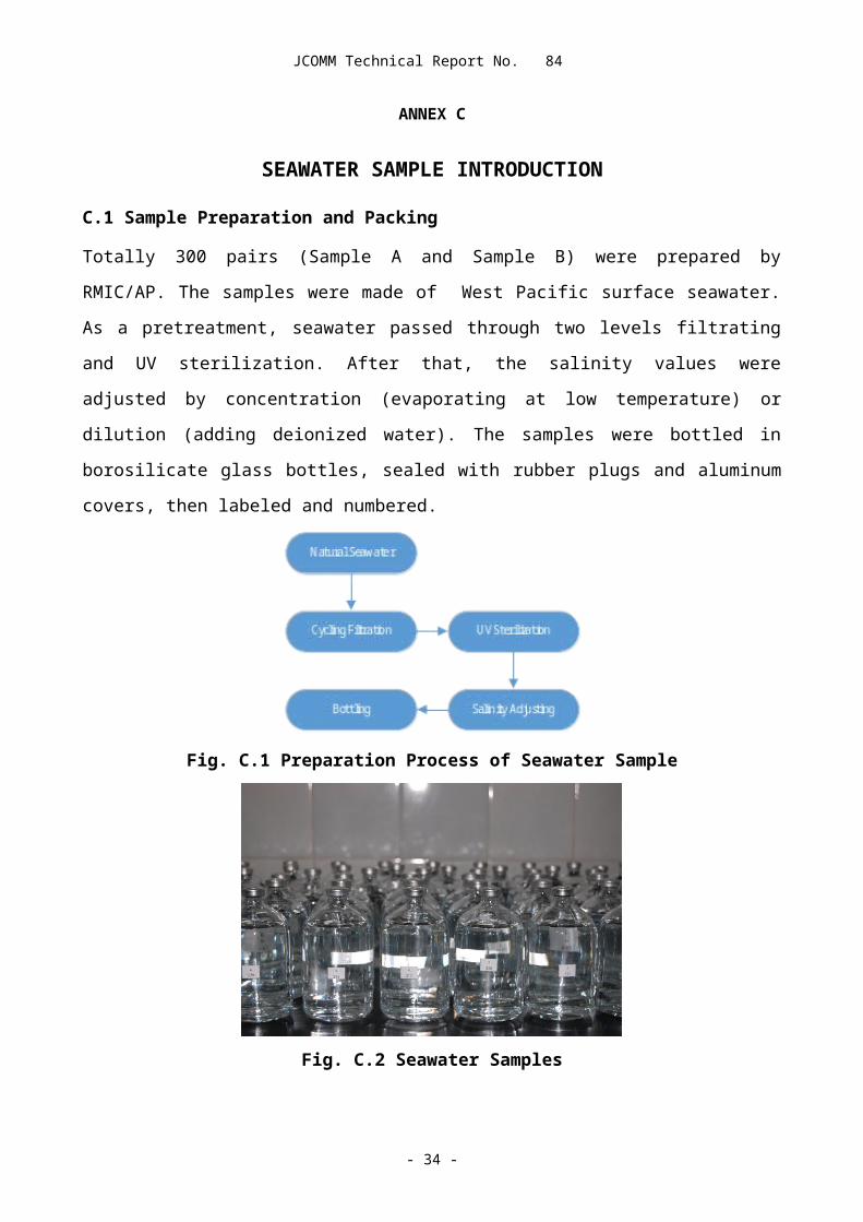
C.1 Sample Preparation and Packing

Totally 300 pairs (Sample A and Sample B) were prepared by RMIC/AP. The samples were made of

West Pacific surface seawater. As a pretreatment, seawater passed through two levels filtrating

and UV sterilization. After that, the salinity values were adjusted by concentration (evaporating at

low temperature) or dilution (adding deionized water). The samples were bottled in borosilicate

glass bottles, sealed with rubber plugs and aluminum covers, then labeled and numbered.

Fig. C.1 Preparation Process of Seawater Sample

Fig. C.2 Seawater Samples

The samples were packaged with waterproof cartons and the gaps were filled with cushion

materials before transportation. The samples were delivered to each participating laboratories via

express shipment. The Operation Guideline, Receipt Form, Laboratory Code and Results Sheet had

been attached to the samples.

Note: RMIC/AP is the manufacturer of Chinese Certified Reference Material for salinity with

certificate number GBW 13150 and GBW (E) 130011.

- 23 -


Fig. C.3 Sample Package, Airway Bill and Permission Report for Transportation

C.2 Homogeneity Test

The standard deviation between bottles and the repeatability standard deviation are calculated for

testing the homogeneity of the sample per ISO GUIDE 35:2006.

Standard deviation between bottles is calculated as below:

sbb=√ MSamong−MSwithin

n (C.1)

The repeatability standard deviation is calculated as follow

sr=√ MSwithin (C.2)

Where:

MSamong—Variance between-bottle;

MSwithin—Variance within-bottle;

n—Measuring times for each sample.

A stratified sampling method is adopted for homogeneity test. 16 groups of sample A and sample

B were picked out. Each group contains 4 bottles where 2 bottles were used to test homogeneity

and the remained 2 bottles were kept as substitutes. Measuring each sample for 3 times on 8400B

Autosal (Cell Temp 24℃,Ambient Temp: 22.5℃, 65%RH)which was standardized with IAPSO SSW

(batch 155), the result of one operator is shown in table C.1

- 24 -


Tab. C.1 Homogeneity Data for Sample A/Sample B

No. Salinity of Sample A No. Salinity of Sample B204 32.5297 32.5297 32.5295 104 24.6971 24.6971 24.6971144 32.5297 32.5297 32.5297 24 24.6971 24.6973 24.6971

4 32.5297 32.5295 32.5295 204 24.6975 24.6975 24.6975284 32.5305 32.5303 32.5305 84 24.6971 24.6969 24.697324 32.5297 32.5295 32.5295 164 24.6971 24.6971 24.6975

224 32.5305 32.5303 32.5301 4 24.6973 24.6973 24.6971304 32.5301 32.5305 32.5305 224 24.6975 24.6975 24.697544 32.5297 32.5295 32.5299 144 24.6973 24.6973 24.6975

124 32.5299 32.5297 32.5299 244 24.6975 24.6975 24.6973244 32.5301 32.5297 32.5299 44 24.6971 24.6973 24.6971164 32.5303 32.5303 32.5299 304 24.6977 24.6977 24.697564 32.5297 32.5295 32.5299 64 24.6971 24.6973 24.6973

184 32.5299 32.5299 32.5299 264 24.6975 24.6975 24.6973104 32.5297 32.5295 32.5297 124 24.6971 24.6975 24.6973264 32.5299 32.5299 32.5301 284 24.6979 24.6977 24.697584 32.5295 32.5299 32.5297 184 24.6973 24.6973 24.6973

One-way analysis of variance (ANOVA) was applied to data analysis, result in table C.2.

sbb and sr are calculated using MSamong and MSwithin. The results are as follows:

sbb ( A )=¿2.53×10-4

sr ( A )=¿1.47×10-4

sbb (B )=¿1.65×10-4

sr ( B )=¿1.32×10-4

Tab. C.2 ANOVA Study

Source of Variation

Salinity of Sample A Salinity of Sample B

SSDegrees

of Freedom

MS SSDegrees

of Freedom

MS

Between-bottle 3.20×10-6 15 2.13×10-7 1.49×10-6 15 9.95×10-8

Within-bottle 6.93×10-7 32 2.17×10-8 5.60×10-7 32 1.75×10-8

Total 3.89×10-6 47 2.05×10-6 47

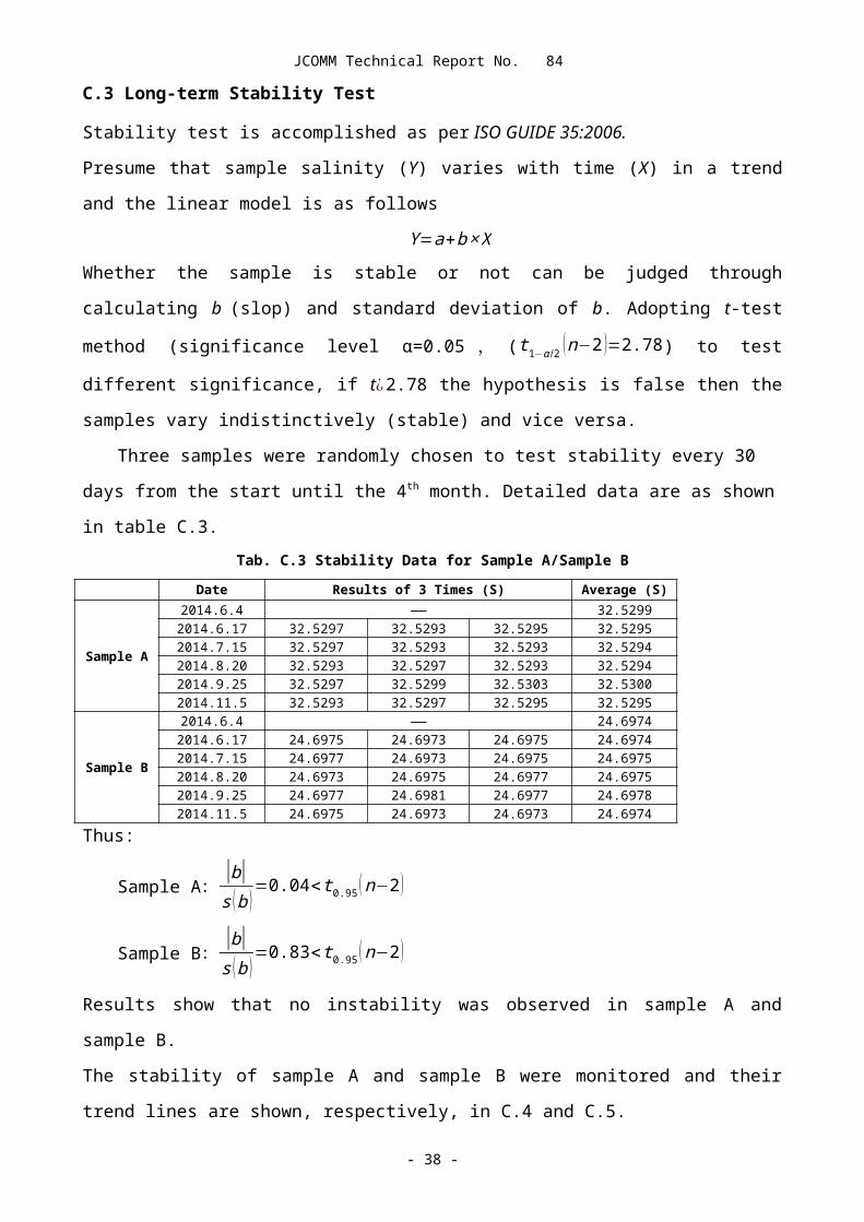
C.3 Long-term Stability Test

Stability test is accomplished as per ISO GUIDE 35:2006.

Presume that sample salinity (Y) varies with time (X) in a trend and the linear model is as follows

Y=a+b× X

Whether the sample is stable or not can be judged through calculating b (slop) and standard

deviation of b. Adopting t-test method (significance level α=0.05 ， (t 1−α /2 (n−2 )=2.78) to test

different significance, if t¿2.78 the hypothesis is false then the samples vary indistinctively (stable)

and vice versa.

- 25 -


Three samples were randomly chosen to test stability every 30 days from the start until the

4th month. Detailed data are as shown in table C.3.

Tab. C.3 Stability Data for Sample A/Sample B

Date Results of 3 Times (S) Average (S)

Sample A

2014.6.4 —— 32.52992014.6.17 32.5297 32.5293 32.5295 32.52952014.7.15 32.5297 32.5293 32.5293 32.52942014.8.20 32.5293 32.5297 32.5293 32.52942014.9.25 32.5297 32.5299 32.5303 32.53002014.11.5 32.5293 32.5297 32.5295 32.5295

Sample B

2014.6.4 —— 24.69742014.6.17 24.6975 24.6973 24.6975 24.69742014.7.15 24.6977 24.6973 24.6975 24.69752014.8.20 24.6973 24.6975 24.6977 24.69752014.9.25 24.6977 24.6981 24.6977 24.69782014.11.5 24.6975 24.6973 24.6973 24.6974

Thus:

Sample A：|b|s ( b )

=0.04< t0.95 (n−2 )

Sample B：|b|s ( b )

=0.83<t 0.95 ( n−2 )

Results show that no instability was observed in sample A and sample B.

The stability of sample A and sample B were monitored and their trend lines are shown,

respectively, in C.4 and C.5.

Fig. C.4 Stability of Sample A

- 26 -


Fig. C.5 Stability of Sample B

C.4 Short-term Stability Test

In order to inspect whether the characteristics value changes or not during transportation and

storage, another batch of 200 bottles of sample were produced following the same manufacture

procedure as that of sample A and sample B. The samples were placed under high temperature,

low temperature and low pressure environment respectively. Then after a period of time,

measuring their salinity values, and compare them with the initial value.

t-test method is used to evaluate the significant difference between the mean value of

measurements before and after environment test. t value calculated as follow:

t=|x1−x2|

√ (n1−1 ) s12+( n2−1 ) s2

2

n1+n2−2 ×n1+n2

n1 n2

Where

： x1 、 x2 is the measured mean value before and after test respectively ， s1 ， s2 is the

standard deviation before and after test respectively，n1，n2 is the number of tested samples。

Comparing t value with t 1−α /2 (n1+n2−1 ) (significance level α=0.05, t 0.975 (15 )=2.1315). If t ＜

t 1−α /2 (n1+n2−1 ) , no significant difference of measured mean value is found between two groups

therefore in this case the samples remain stable after experiencing special environments.

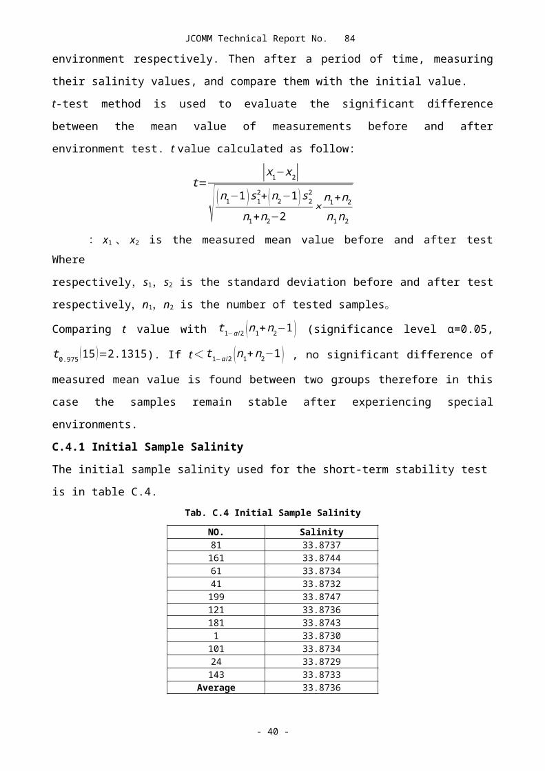
C.4.1 Initial Sample Salinity

The initial sample salinity used for the short-term stability test is in table C.4.

Tab. C.4 Initial Sample Salinity

- 27 -


C.4.2 High Temperature Environmental Test

Samples were placed in 55°C environment for 7 days (168h) and 10 days (240h), respectively. Then

the salinity values of these samples were measured. The measurement results and corresponding

t-test results are listed in the following table:

Tab. C.5 Results of High Temperature Environmental Test (7 days)

Test Results Initial Salinity t Value Critical t Value

No. Salinity

33.8736 0.6255 2.1315

69 33.873137 33.8729

158 33.8737127 33.8737187 33.873794 33.8735

Average 33.8734Tab. C.6 Results of High Temperature Environmental Test (10 days)

Test Results Initial Salinity t Value Critical t ValueNo. Salinity

33.8736 1.3959 2.1315

66 33.8731151 33.8739

4 33.872736 33.8727

124 33.873796 33.8731

Average 33.8732

Results show that after storing in high temperature for a period time, the sample salinity did not

change significantly.

C.4.3 Low Temperature Environmental Test

Samples were placed in 5°C environment for 7 days (168h) and 10 days (240h) respectively. Then

the salinity values of these samples were measured. The measurement results and corresponding

t-test results are listed in the following table:

Tab. C.7 Results of Low Temperature Environmental Test (7 days)

Test Results Initial Salinity t Value Critical t ValueNo. Salinity 33.8736 0.2484 2.1315104 33.8735

- 28 -

NO. Salinity81 33.8737

161 33.874461 33.873441 33.8732

199 33.8747121 33.8736181 33.8743

1 33.8730101 33.873424 33.8729

143 33.8733Average 33.8736


35 33.8731139 33.873956 33.8731

180 33.873985 33.8737

Average 33.8735Tab. C.8 Results of Low Temperature Environmental Test (10 days)

Test Results Initial Salinity t value Critical t valueNo. Salinity

33.8736 1.1381 2.1315

103 33.873380 33.8731

188 33.873918 33.8727

147 33.873952 33.8727

Average 33.8733

Results show that after storing in low temperature for a period time, the sample salinity did not


C.4.4 Low Pressure Environmental Test

The samples were stored at the pressure of -0.05MPa for one day. Then the salinity values of

these samples were measured. The measurement results and corresponding t-test results are

listed in the following table:

Tab. C.9 Results of Low Pressures Environmental Test

Test Results Initial Salinity t Value Critical t ValueNo. Salinity

33.8736 0.2276 2.5706

126 33.874120 33.8727

191 33.874183 33.873765 33.8733

100 33.8733Average 33.8735

Results show that after storing at low pressure for a period time, the sample salinity did not


C.4.5 Impact & Vibration Test

The well-packed samples were put on the impact and vibration test equipment, after test no

damages were found on both bottles and the packages.

____________

- 29 -


ANNEX D

JCOMM PILOT INTERCOMPARISON PROJECT FOR SEAWATER SALINITY MEASUREMENTS

OPERATIONS GUIDELINE

Welcome to take part in this salinity intercomparison activity!

To ensure this activity goes smooth, every participant should start reading and understanding these Guidelines and the annexed documents below carefully:

Annex 1: RECEIPT FORMAnnex 2: RESULTS SHEET

D.1 SAMPLES

Two seawater samples, labelled as Sample-1 and Sample-2, sealed in pharmaceutical-grade borosilicate glass bottles with volume of ca.220ml, will be distributed. One of the samples has an unknown salinity value between 20 and 25 and the other one has an unknown salinity value between 30 and 35.

After receiving the samples, please unpack the samples and check their integrity immediately. Then, fill out the RECEIPT FORM and send it back via fax or email (using a scanning copy) to the designated RMIC/AP contact point (see annex 1 for contact details) within two work days; In case that any sample is NOT in intact condition (broken or leaking), please paste a photo in the RECEIPT FORM before sending it back. RMIC/AP will ship another pair of samples as soon as possible.

D.2 SAMPLE TESTING

The intercomparison samples should be treated as routine laboratory samples. Where possible, please record the method used and attach it to the RESULTS SHEET.

Caution: The samples must be tested as soon as the bottles are opened.

D.3 SAFETY

The samples should only be used for this intercomparison activity by the participating laboratories.

Caution: The samples are made from natural seawater and are corrosive to metals.

D.4 RESULTS REPORTING

1.1 Please send the RESULTS SHEET with original measuring records via fax or email (using a scanning copy) to the designated RMIC/AP contact point NO LATER THAN July 15th 2014;

1.2 The results should be reported in the form of practical salinity per PSS-78, to 3 decimal places;

- 30 -


1.3 For each sample, three measuring results and the average should be reported;

1.4 Where possible, every participant should assess the measurement uncertainty associated with the testing of each sample (with confidential probability of 95% or coverage factor k=2) per ISO GUM, and provide the procedures of assessment;

1.5 Please DO NOT juggle any of the measuring results.

D.5 CONFIDENTIALITY

To keep the confidentiality of this activity, each participant will be randomly assigned an ID code which is shown on the RESULTS SHEET. In the final report, all participants will be represented by their ID codes if necessary.

- 31 -


Annex 1

RECEIPT FORM OF SAMPLES

Participant ID Code:

PT Plan Salinity Measurement

Activity Sponsor JCOMM

Sample Distributor RMIC-AP

Designated RMIC/AP contact

points

Ya’nan Li, Bo Zhang

Phone/Fax +86-22-27539531/+86-22-27539530

E-mail [email protected]

Sample Shipping Date

Participant:

Mailing Address:

Contact point E-mail:

Phone:

Fax:

The samples were received on:(Date)

By: (Signature)

Is any sample damaged? (Yes/ No)

If yes, please attach a photo here:

Have your laboratory involved in (or prepare to involve in) any marine/ocean

observation programmes of JCOMM? (Yes/ No)

If yes, please provide the programme name:

- 32 -

×××


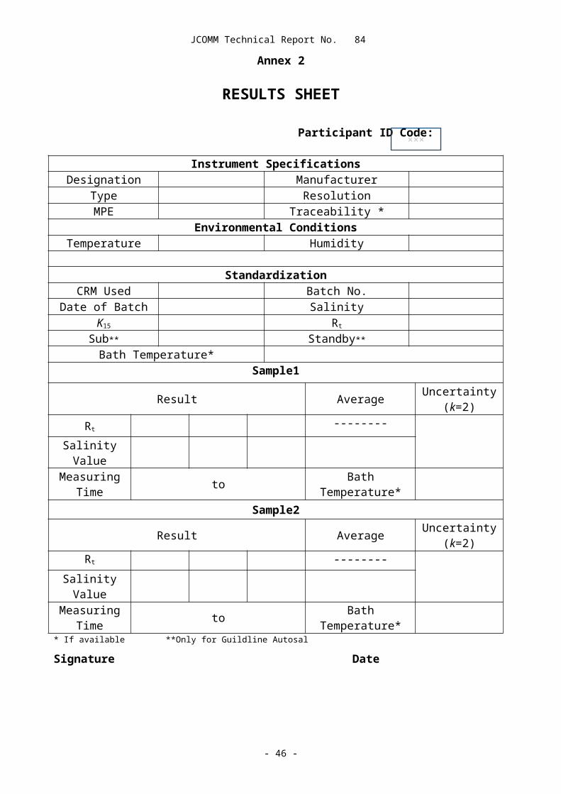
Annex 2

RESULTS SHEET

Participant ID Code:

Instrument SpecificationsDesignation Manufacturer

Type ResolutionMPE Traceability *

Environmental ConditionsTemperature Humidity

StandardizationCRM Used Batch No.

Date of Batch SalinityK15 Rt

Sub** Standby**

Bath Temperature*Sample1

Result Average Uncertainty (k=2)

Rt--------

Salinity Value

Measuring Time to Bath Temperature*

Sample2

Result Average Uncertainty (k=2)

Rt --------

Salinity Value

Measuring Time to Bath Temperature*

* If available **Only for Guildline Autosal

Signature Date

- 33 -

×××


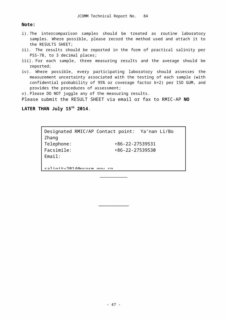
Note:

i). The intercomparison samples should be treated as routine laboratory samples. Where possible, please record the method used and attach it to the RESULTS SHEET;

ii). The results should be reported in the form of practical salinity per PSS-78, to 3 decimal places;iii). For each sample, three measuring results and the average should be reported;iv). Where possible, every participating laboratory should assesses the measurement uncertainty associated

with the testing of each sample (with confidential probability of 95% or coverage factor k=2) per ISO GUM, and provides the procedures of assessment;

v). Please DO NOT juggle any of the measuring results.Please submit the RESULT SHEET via email or fax to RMIC-AP NO LATER THAN July 15th 2014.

____________

____________

- 34 -

Designated RMIC/AP Contact point: Ya’nan Li/Bo ZhangTelephone: +86-22-27539531Facsimile: +86-22-27539530Email: [email protected] Address: 219 W. Jieyuan Rd

Nankai, Tianjin, 300112China


ANNEX E

INTRODUCTION OF MEASURING INSTRUMENTS USED IN THE PROJECT

Majority of participants used laboratory salinometer from Guildline and OPTIMARE in the project.

Minority of laboratories used hand-held portable instruments to measure seawater samples.

Three different brands were concerned. They are YSI, ELMETRON and ATAGO. Some brief

introductions of the up mentioned products from manufacturers are shown below.

E.1 Guildline 8400B Autosal Salinometer

Fig. E.1 Guildline 8400B Autosal Lab Salinometer

Guildline 8400B Autosal Lab Salinometer manufactured by Guildline (Canada) is a precise

salinometer generally used around the world. The specifications are shown in Table E.1, for more

details please browse website:

http://www.guildline.com/oceanography.php.

Tab. E.1 General Specifications of 8400B Salinometer

No. Items Specifications

1 Measurement Range0.0001:1.15 Conductivity Ratio0.004 to 76mS/cm2 to 42 Equivalent Practical Salinity Units (PSU)

2 Accuracy <±0.0001 Conductivity Ratio, @same set point temperature as

- 35 -



standardization and within -2 and +4 of ambient.℃ ℃By calculation & substitution in the Bennett equation or the UNESCO tables,< ± 0.002 Equivalent PSU.

3 Short Term Stability < ± 0.00005 for 24 hours without restandardization

4 Maximum Resolution< 0.00001 Conductivity Ratio< 0.0002 mS/cm @15 and 35 PSU℃< 0.0002 Equivalent PSU

E.2 Guildline 8410A Portasal Salinometer

Fig E.2 Guildline 8410A Portasal Salinometer

Guildline 8410A Portasal Salinometer manufactured by Guildline (Canada) is a precise salinometer

generally used around the world. It is applicable to laboratory on ship board. The specifications are

shown in Table E.2, for more details please browse website:


Tab. E.2 General Specifications of 8410A Salinometer

No. Items Specifications

1 Measurement Range 0.004 to 76 mS/cm0.0001:1.15 Conductivity Ratio

2 Accuracy ± 0.003 Equivalent PSU @same set point temperature as standardization and within -2 and +4 of ambient℃ ℃

3 Resolution: 0.0003mS/cm @15 and 35 PSU℃0.0003 Equivalent PSU

4 Temperature stability ± 0. 001℃

- 36 -

http://www.guildline.com/oceanography.php.%20


E.3 Guildline 8400A Autosal Salinometer

Fig. E.3 Guildline 8400A Autosal Salinometer

Guildline 8400A Autosal Salinometer manufactured by Guildline (Canada) is the last generation

product of 8400B and is out of production for the present. It has a 4 electrode cell which measures

the conductivity ratio of a seawater sample in less than one minute. The salinity range of the

instrument is about 0.005-42 and has a stated accuracy of ±0.003 by the manufacturer.

E.4 OPTIMARE Precision Salinometer

Fig E.4 OPTIMARE Precision Salinometer

OPTIMARE Precision Salinometer (OPS) is a brand new product manufactured by OPTIMARE

(Germany) which is applicable to laboratory or for ship board use, the detailed specifications are

listed in TableE.3.

For more information please browse the following website:

http://www.optimare.de/cms/en/divisions/mms/mms-products/precision-salinometer.html

Tab. E.3 General Specifications of OPTIMARE Salinometer

- 37 -

http://www.optimare.de/cms/en/divisions/mms/mms-products/precision-salinometer.html


Mechanical PropertiesDimensions 688 mm x 476 mm x 350 mm, packed in Zagreb aluminum box

Mass 30 kg instrument + 13.5 kg waterWater bath volume Main-bath: 13 l Pre-bath: 0.5 l

SensorsConductivity Modified Sea-Bird Electronics SBE 4

Temperature, main bath Sea-Bird Electronics SBE 3plusSalinity accuracy 0.001 or better

Data acquisitionData storage Hard disk and USB memory stick

User interface Touch screen (with optional USB keyboard/mouse)Power supply

Current 4 AVoltage 100 V to 240 V; 50 Hz to 60 Hz

E.5 YSI Professional Plus Handheld Multi-parameter

Fig. E.5 YSI Professional Plus Handheld Multi-parameter

Manufactured by the YSI Company in U.S.A, YSI’s Professional Plus handheld multi-parameter

water quality instrument allows up to four probes (5 parameters plus barometric pressure). The

available options of parameters include DO, pH, conductivity, ORP, Ammonium, Chloride, and

Nitrates. Salinity measurements are derived from measured conductivity. The measurement range

of salinity is from 0 to 70ppt with the accuracy of ±1% or 0.1ppt. The resolution is 0.01ppt. For

more information please browse the following website: http://www.ysi.com.

- 38 -

http://www.ysi.com/


E.6 ELMETRON CPC401

Fig. E.6 ELMETRON CPC401

Manufactured by the ELMETRON Company in Poland, CPC-401 can be used for both field and

laboratory measurements of conductivity/salinity. The measurement range of conductivity is from

0 to 1999.9 mS/cm with the accuracy of ±0.25%F.S

(＞20 mS/cm). The temperature compensation is carried out. The conductivity measurement can

be converted into salinity in NaCl (0~250 g/l) or KCl (0~200 g/l).

For more information please browse the following website: http://www.elmetron.pl/.

E.7 ATAGO Hand-Held Refractometer S/Mill-E

Fig. E.7 ATAGO Hand-Held Refractometer S/Mill-E

Manufactured by the ATAGO Company in Japan, Refractometer S/Mill-E measures the salinity

which is displayed in parts per mill (‰). The measurement range is from 0 to 100‰. The

temperature compensation is carried out manually.

For more information please browse the following website: http://www.atago.net

- 39 -

http://www.atago.net./

http://www.elmetron.pl/


Tab. E.4 General Specifications of ATAGO Hand-Held Refractometer S/Millα

Model MASTER-S/MillαCat.No. 2491

Scale SalinitySpecific gravity

Measurement RangeSalinity : 0 to 100‰

Specific gravity : 1.000 to 1.070(Automatic Temperature Compensation)

Minimum Scale Salinity : 1‰Specific gravity : 0.001

Measurement AccuracySalinity : ±2‰

Specific gravity : ±0.001(10 to 30°C)

International Protection Class IP65 (except eye piece)Dust-tight and Protected against water jets.

Dimensions & Weight 3.2×3.4×20.7cm, 110g

____________

- 40 -


ANNEX F

EXAMPLE FOR UNCERTAINTY EVALUATION OF SALINITY MEASUREMENT RESULT

An example is set here below to introduce the method of uncertainty evaluation by using Guildline

8400B Autosal salinometer to measure salinity of seawater samples (For reference).

F.1 Measuring Method

Salinometer is standardized with SSW of 35 and linear-corrected with series SSW pack before

measurement. Conductivity ratio is the mean value of measurement results for 3 times. Salinity is

calculated with conductivity ratio applying PSS-78 formula.

F.2 Measurement Model

Considering influence of the accuracy of the salinometer, SSW, linearity correction and PSS-78

fitting formula, final salinity S can be expressed as below

S=S t+δr+δssw+δPSS （F.1）

Where：

St—Measured salinity value from salinometer

δ r—Measurement repeatability.

δ ss w—Influence of SSW accuracy

δPSS—Influence of fitting accuracy of PSS-78 formula

F.3 Component Uncertainty Evaluation

F.3.1 Measured Salinity,St

i) If linearity correction is not performed, the accuracy of 8400B is with respect to the information

from manufacturer (see 4.1) which is better than±0.002. Presume that the distribution accords

with rectangular model, thus the uncertainty of measured salinity is as follows

ust=0.002

√3=1.2×10−3

ii) If the salinometer is calibrated before measurement (ex. linearity-corrected with SSW pack), the

uncertainty of the measurement is equal to the uncertainty on the certificate. Hereby, presume

that SSW pack (10, 30, 38) was used for calibration, then the expanded uncertainty of the

calibrated result is U=1.1×10-3 (k=2). And the uncertainty of measured salinity by using salinometer

is

ust'=

0.00112

=5.5 ×10−4

F.3.2 Repeatability, δr

- 41 -


Considering stability of salinometer, the standard deviation of measurements s(x) is calculated by

past data. s(x)=2.5×10-4 , then standard deviation of mean value of 3 times measurement is

calculated as follows:

uδr=sP

√n=0.00025

√3=1.5 ×10−4

F.3.3 Influence of SSW Accuracy,δssw

SSW is used for standardization. U=0.001 (k=2)

uδssw=0.001

2=5 ×10−4

F.3.4 Influence of Fitting Accuracy of PSS-78 Formula，δPSS

The standard deviation introduced by PSS-78 fitting formula is 0.0007 (Perkin, R. G. and Lewis, E.

L., 1980)

uδPSS=7 ×10−4

Note: Le Menn, M. (2011) brought this component uncertainty into the evaluation process of

salinity measurement which leads to an expanded uncertainty of 0.0022. However, this

component uncertainty is neglected by others. Since this component uncertainty could be seen as

a generally existing effect, there still need agreement on whether to bring it into the uncertainty

evaluation or not. This effect was not taken into consideration here.

F.4 Uncertainty Budget

Component uncertainties of salinity measurement result are listed in table F.2

Tab. F.2 Summary Sheet of Component Uncertainty

QuantityXi

Estimatexi

Standard Uncertainty

u(xi)

Probability Distribution

Sensitivity Coefficient

ci

Uncertainty Contributionu(yi)

St/St ' 32.530 1.2×10-3*5.5×10-4** normal 1 1.2×10-3*

5.5×10-4**δr 0 1.5×10-4 rectangular 1 5.8×10-4

δssw 0 5×10-4 normal 1 5×10-4

S 32.530 \ normal \ 1.5×10-3*1.0×10-3**

Note: * salinometer without calibration; **salinometer after calibration

F.5 Expanded Uncertainty

The uncertainty of measurement is estimated to comply with normal distribution and the freedom

degree is big enough. The coverage factor is k=2 and the corresponding probability is 95%. Then

- 42 -


U=0.0015×2=0.003 (salinometer without calibration) and U=0.001×2=0.002 (salinometer after

calibration).

F.6 Uncertainty Report

The expanded uncertainty of the measurement are as follows:

i) U=0.003, k=2 (salinometer without calibration);

ii) U=0.002, k=2 (salinometer after calibration).

____________

- 43 -


ANNEX G

LIST OF ACRONYMS

Argo International profiling float programme (not an acronym)AWI Alfred-Wegener-Institut Helmholtz Zentrum fur Polar und Meeresforschung (Germany)BSH Bundesamt fur Seeschiffahrt und Hydrographie (Germany)CIMO Commission on Instruments and Methods of Observation (WMO)CSIRO Commonwealth Scientific and Industrial Research Organisation (Australia)DBCP Data Buoy Co-operation Panel (WMO-IOC)FMS Faculty of Marine Sciences (Pakistan)GEOMAR GEOMAR Helmholtz Centre for Ocean Research (Germany)GLOSS Global Sea-level Observing System (JCOMM)GOOS Global Ocean Observing System (IOC, WMO, UNEP, ICSU)GO-SHIP Global Ocean Ship-Based Hydrographic Investigations ProgrammeGUM Guide to the Expression of Uncertainty in MeasurementIAPSO International Association for the Physical Sciences of the OceansICSU International Council for ScienceID Identification NumberIEC International Electrotechnical CommissionIFREMER French Research Institute for Exploitation of the SeaIMA Institute of Marine Affairs (Trinidad & Tobago)IMR Institute of Marine Research (Norway)IMSF Institute of Marine Sciences and Fisheries (Bangladesh)IOC Intergovernmental Oceanographic Commission of UNESCOIOCCP International Ocean Carbon Coordination Project of IOCISMAR CNR-ISMAR Institute of Marine Science- U.O.S. Pozzuolo di Lerici (Italy)ISO International Organization for StandardizationJCOMM Joint WMO-IOC Technical Commission for Oceanography and Marine MeteorologyKIOST Korea Institute of Ocean Science & TechnologyKMS Kenya Meteorological ServiceLUAWMS Lasbela University of Agriculture, Water and Marine Sciences (Pakistan)MPE Maximum permissible errorsNCOSM SOA National Centre of Ocean Standards and Metrology (China)NIO National Institute of Oceanography (India)NIO National Institute of Oceanography (Pakistan)NIWA National Institute of Water and Atmospheric Research (New Zealand)NOC National Oceanography Centre (United Kingdom)OC Organizing CommitteeOceanSITES OCEAN Sustained Interdisciplinary Timeseries Environment observation SystemOCG Observations Coordination Group (JCOMM)OGS Istituto Nazionale di Oceanografia e di Geofisica Sperimentale (Italy)OMICS KIOST Oceanographic Measurement & Instrument Calibration Service CenterOSIS Ocean Science and Information Services，Marine Institute (Ireland)PSU Practical Salinity UnitQA Quality AssuranceQC Quality ControlQM Quality ManagementRBINS Royal Belgian Institute of Natural Sciences-OD Nature – MARCHEM (Belgium)RMIC WMO-IOC Regional Marine Instrument CentreRMIC/AP RMIC for the Asia Pacific regionRMS Root Mean SquareSCSEMC South China Sea Environmental Monitoring Center (SCSEMC) (China)SHOM French Naval Hydrographic and Oceanographic ServiceSIO Scripps Institution of Oceanography (University of California, USA)SOA State Oceanic Administration (China)SOT Ship Observations Team (JCOMM)SST Sea-Surface TemperatureSSW Standard SeawaterToR Terms of ReferenceUN United NationsUNEP United Nations Environment Programme

- 44 -


UNESCO United National Educational, Scientific and Cultural OrganizationUSA United States of AmericaWCRP World Climate Research Programme WG Working GroupWHOI Woods Hole Oceanographic InstitutionWIGOS WMO Integrated Global Observing SystemWMO World Meteorological Organization (UN)WWW World Weather Watch (WMO)XBT Expendable BathyThermographXCTD Expendable Conductivity/Temperature/Depth

____________

- 45 -



- 46 -

Documents

JCOMM TR No. 84 - Seawater Salinity Intercomparison Pilor …€¦ · Web view · 2016-11-29Final Report, JCOMM Pilot Intercomparison Project for Seawater Salinity Measurements