Embed Size (px)
Citation preview
January 31, 2006 AI: Chapter 4: Informed Search and Exploration
1
Artificial IntelligenceChapter 4: Informed Search
and Exploration
Michael SchergerDepartment of Computer
ScienceKent State University
January 31, 2006 AI: Chapter 4: Informed Search and Exploration
2
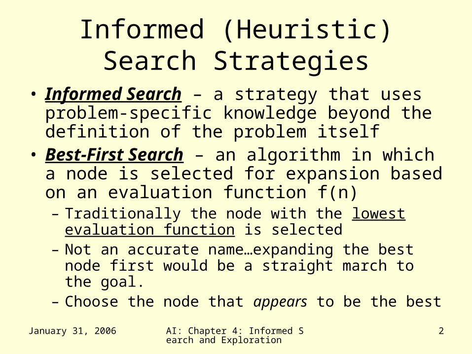
Informed (Heuristic) Search Strategies
• Informed Search – a strategy that uses problem-specific knowledge beyond the definition of the problem itself
• Best-First Search – an algorithm in which a node is selected for expansion based on an evaluation function f(n)– Traditionally the node with the lowest
evaluation function is selected – Not an accurate name…expanding the best
node first would be a straight march to the goal.
– Choose the node that appears to be the best
January 31, 2006 AI: Chapter 4: Informed Search and Exploration
3
Informed (Heuristic) Search Strategies
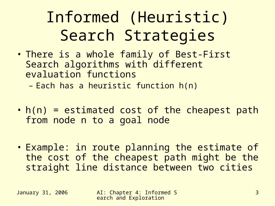
• There is a whole family of Best-First Search algorithms with different evaluation functions– Each has a heuristic function h(n)
• h(n) = estimated cost of the cheapest path from node n to a goal node
• Example: in route planning the estimate of the cost of the cheapest path might be the straight line distance between two cities
January 31, 2006 AI: Chapter 4: Informed Search and Exploration
4
A Quick Review
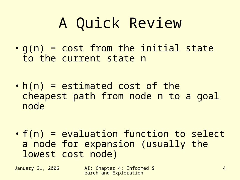
• g(n) = cost from the initial state to the current state n
• h(n) = estimated cost of the cheapest path from node n to a goal node
• f(n) = evaluation function to select a node for expansion (usually the lowest cost node)
January 31, 2006 AI: Chapter 4: Informed Search and Exploration
5
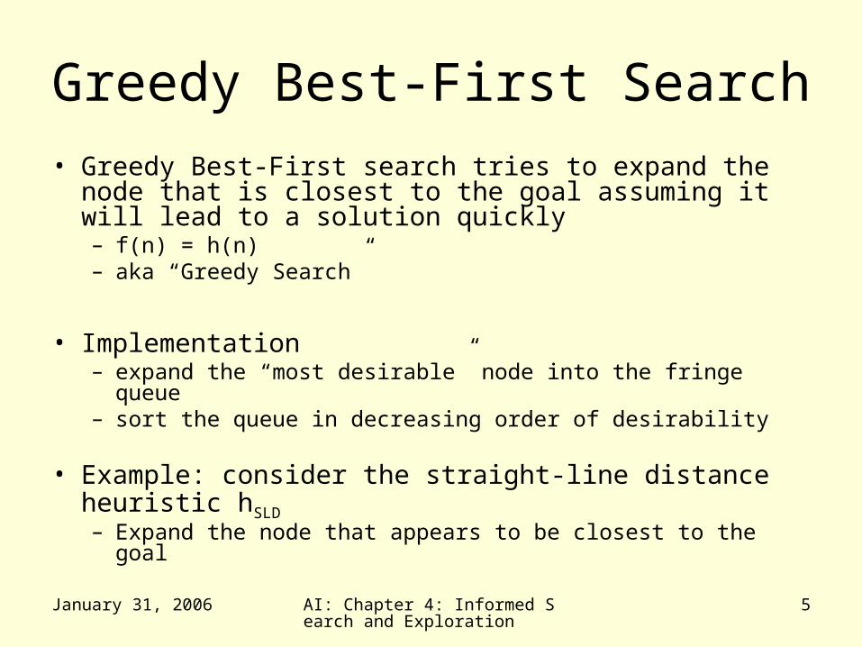
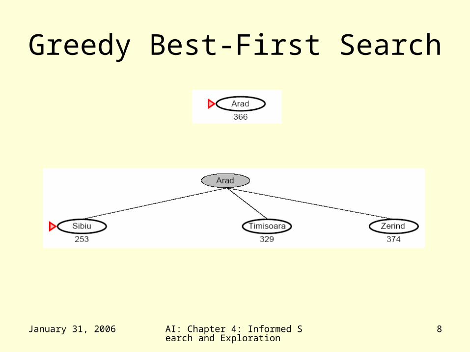
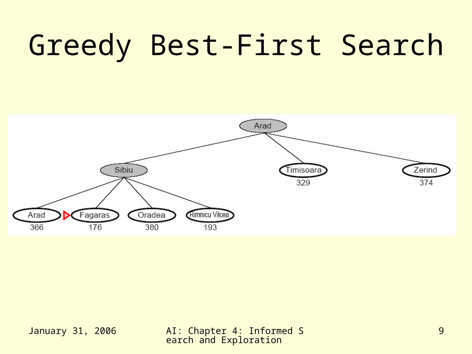
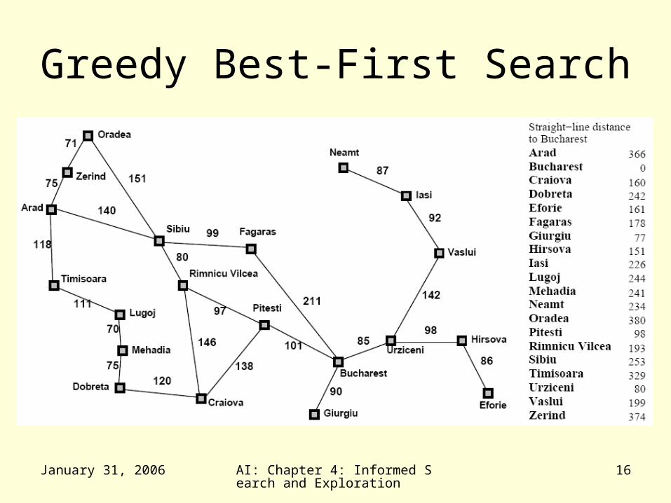
Greedy Best-First Search• Greedy Best-First search tries to expand the node
that is closest to the goal assuming it will lead to a solution quickly– f(n) = h(n)– aka “Greedy Search”
• Implementation– expand the “most desirable” node into the fringe queue– sort the queue in decreasing order of desirability
• Example: consider the straight-line distance heuristic hSLD– Expand the node that appears to be closest to the goal

January 31, 2006 AI: Chapter 4: Informed Search and Exploration
6
Greedy Best-First Search
January 31, 2006 AI: Chapter 4: Informed Search and Exploration
7
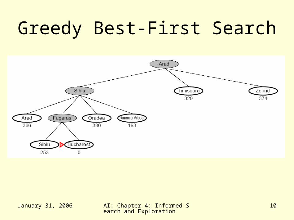
Greedy Best-First Search
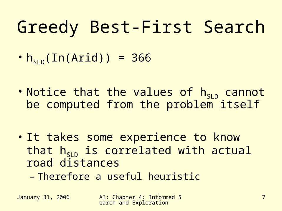
• hSLD(In(Arid)) = 366
• Notice that the values of hSLD cannot be computed from the problem itself
• It takes some experience to know that hSLD is correlated with actual road distances– Therefore a useful heuristic
January 31, 2006 AI: Chapter 4: Informed Search and Exploration
8
Greedy Best-First Search
January 31, 2006 AI: Chapter 4: Informed Search and Exploration
9
Greedy Best-First Search
January 31, 2006 AI: Chapter 4: Informed Search and Exploration
10
Greedy Best-First Search
January 31, 2006 AI: Chapter 4: Informed Search and Exploration
11
Greedy Best-First Search
• Complete– No, GBFS can get stuck in loops (e.g. bouncing
back and forth between cities)
• Time– O(bm) but a good heuristic can have dramatic
improvement
• Space– O(bm) – keeps all the nodes in memory
• Optimal– No!
January 31, 2006 AI: Chapter 4: Informed Search and Exploration
12
A Quick Review - Again
• g(n) = cost from the initial state to the current state n
• h(n) = estimated cost of the cheapest path from node n to a goal node
• f(n) = evaluation function to select a node for expansion (usually the lowest cost node)
January 31, 2006 AI: Chapter 4: Informed Search and Exploration
13
A* Search
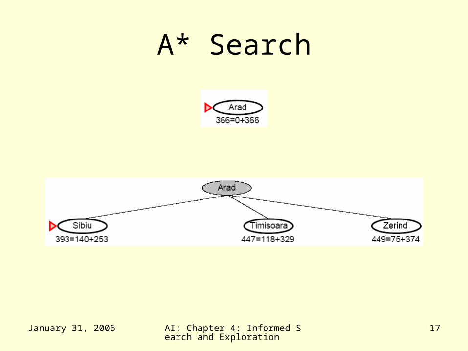
• A* (A star) is the most widely known form of Best-First search– It evaluates nodes by combining g(n)
and h(n)– f(n) = g(n) + h(n)– Where
• g(n) = cost so far to reach n• h(n) = estimated cost to goal from n• f(n) = estimated total cost of path through n
January 31, 2006 AI: Chapter 4: Informed Search and Exploration
14
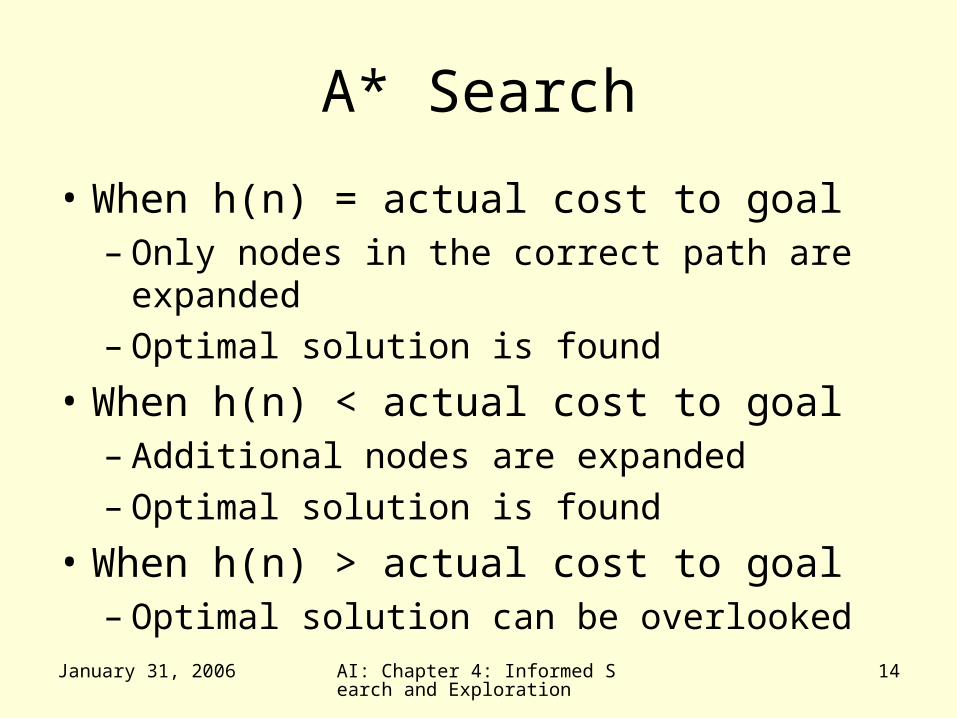
A* Search
• When h(n) = actual cost to goal– Only nodes in the correct path are
expanded– Optimal solution is found
• When h(n) < actual cost to goal– Additional nodes are expanded– Optimal solution is found
• When h(n) > actual cost to goal– Optimal solution can be overlooked
January 31, 2006 AI: Chapter 4: Informed Search and Exploration
15
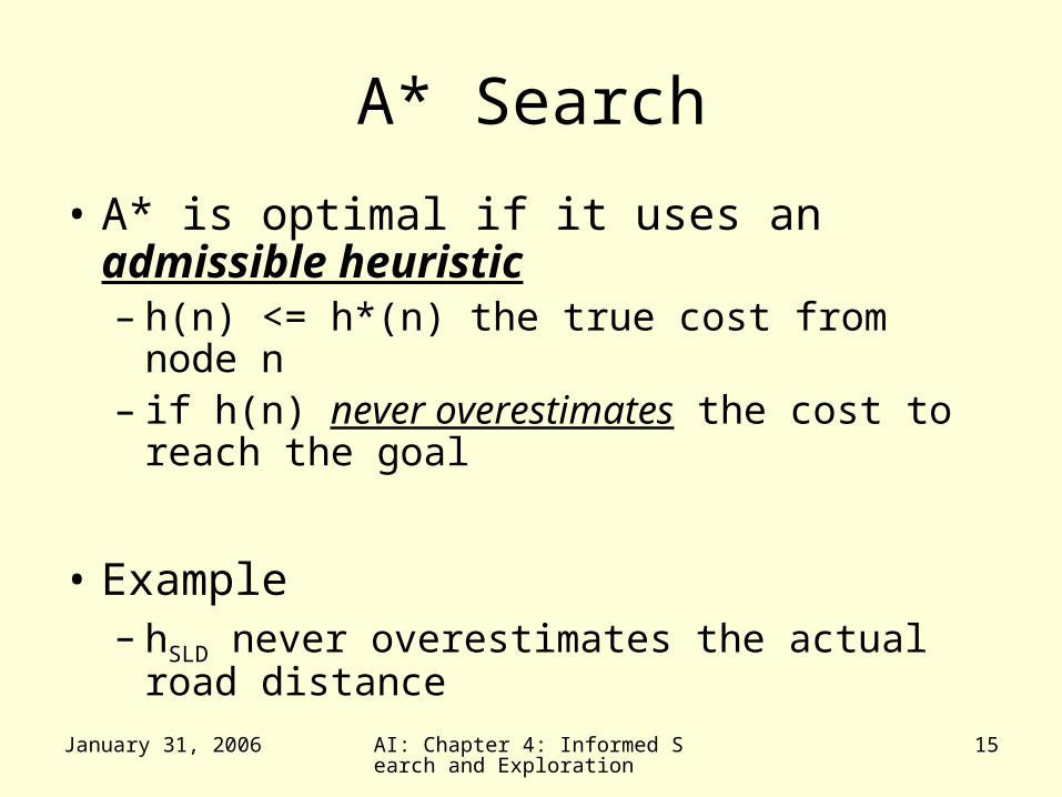
A* Search
• A* is optimal if it uses an admissible heuristic– h(n) <= h*(n) the true cost from node n– if h(n) never overestimates the cost to
reach the goal
• Example– hSLD never overestimates the actual road
distance
January 31, 2006 AI: Chapter 4: Informed Search and Exploration
16
Greedy Best-First Search
January 31, 2006 AI: Chapter 4: Informed Search and Exploration
17
A* Search
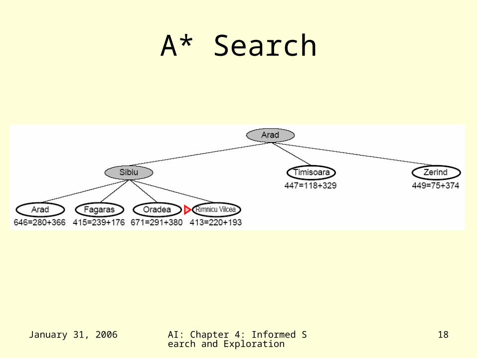
January 31, 2006 AI: Chapter 4: Informed Search and Exploration
18
A* Search
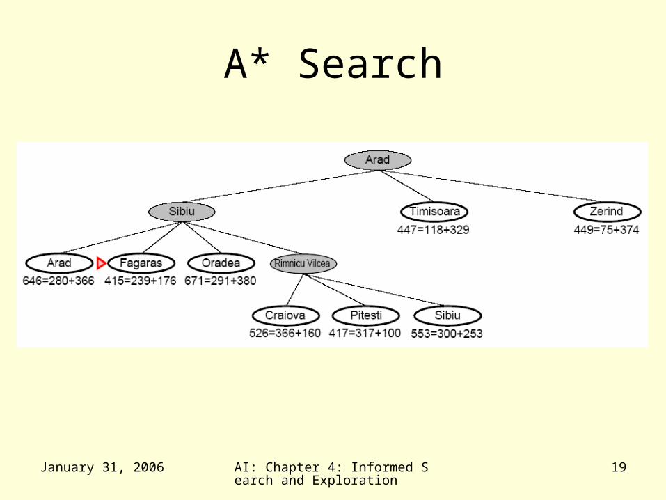
January 31, 2006 AI: Chapter 4: Informed Search and Exploration
19
A* Search
January 31, 2006 AI: Chapter 4: Informed Search and Exploration
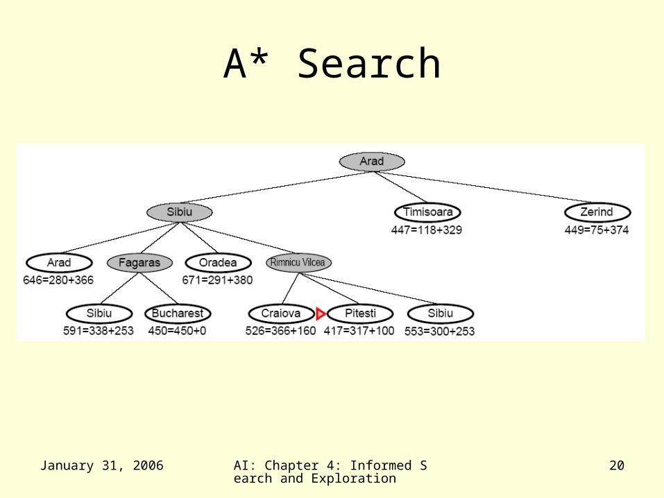
20
A* Search
January 31, 2006 AI: Chapter 4: Informed Search and Exploration
21
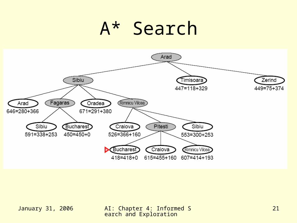
A* Search
January 31, 2006 AI: Chapter 4: Informed Search and Exploration
22
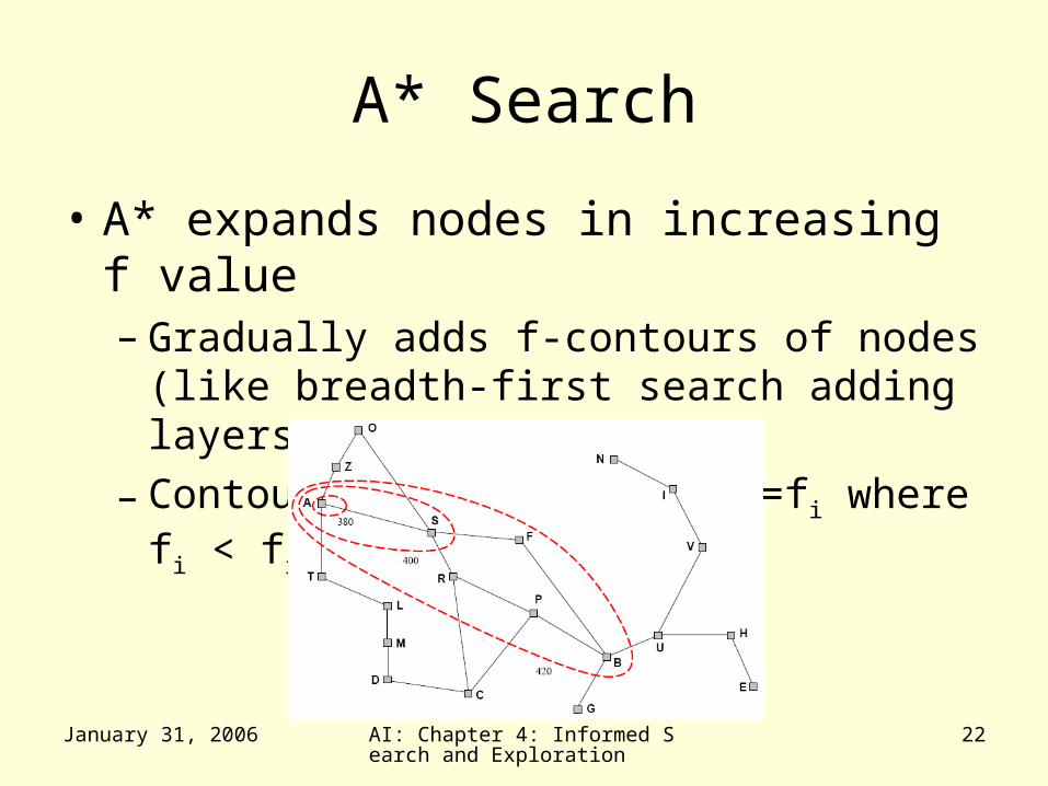
A* Search
• A* expands nodes in increasing f value– Gradually adds f-contours of nodes (like
breadth-first search adding layers)
– Contour i has all nodes f=fi where fi < fi+1
January 31, 2006 AI: Chapter 4: Informed Search and Exploration
23
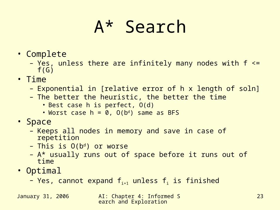
A* Search• Complete
– Yes, unless there are infinitely many nodes with f <= f(G)• Time
– Exponential in [relative error of h x length of soln]– The better the heuristic, the better the time
• Best case h is perfect, O(d)• Worst case h = 0, O(bd) same as BFS
• Space– Keeps all nodes in memory and save in case of repetition– This is O(bd) or worse– A* usually runs out of space before it runs out of time
• Optimal– Yes, cannot expand fi+1 unless fi is finished
January 31, 2006 AI: Chapter 4: Informed Search and Exploration
24
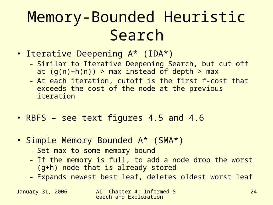
Memory-Bounded Heuristic Search
• Iterative Deepening A* (IDA*)– Similar to Iterative Deepening Search, but cut off at (g(n)
+h(n)) > max instead of depth > max– At each iteration, cutoff is the first f-cost that exceeds
the cost of the node at the previous iteration
• RBFS – see text figures 4.5 and 4.6
• Simple Memory Bounded A* (SMA*)– Set max to some memory bound– If the memory is full, to add a node drop the worst (g+h)
node that is already stored– Expands newest best leaf, deletes oldest worst leaf
January 31, 2006 AI: Chapter 4: Informed Search and Exploration
25
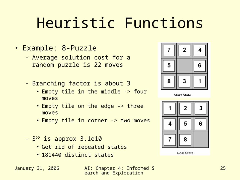
Heuristic Functions
• Example: 8-Puzzle– Average solution cost for a random
puzzle is 22 moves
– Branching factor is about 3• Empty tile in the middle -> four
moves• Empty tile on the edge -> three
moves• Empty tile in corner -> two moves
– 322 is approx 3.1e10• Get rid of repeated states• 181440 distinct states
January 31, 2006 AI: Chapter 4: Informed Search and Exploration
26
Heuristic Functions
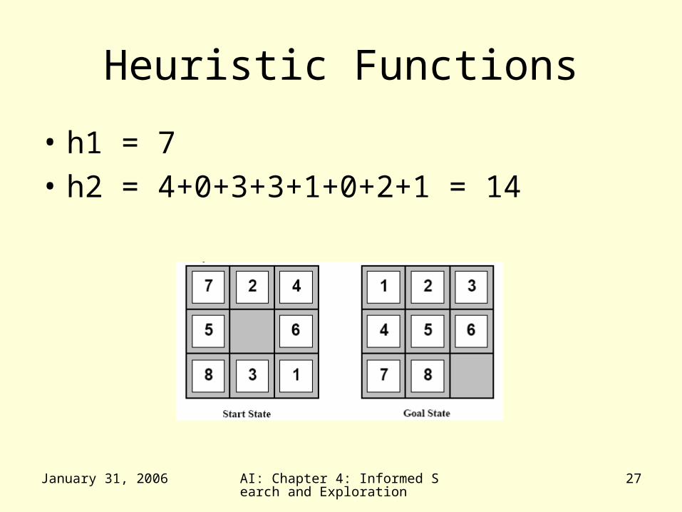
• To use A* a heuristic function must be used that never overestimates the number of steps to the goal
• h1=the number of misplaced tiles
• h2=the sum of the Manhattan distances of the tiles from their goal positions
January 31, 2006 AI: Chapter 4: Informed Search and Exploration
27
Heuristic Functions
• h1 = 7• h2 = 4+0+3+3+1+0+2+1 = 14
January 31, 2006 AI: Chapter 4: Informed Search and Exploration
28
Dominance
• If h2(n) > h1(n) for all n (both admissible) then h2(n) dominates h1(n) and is better for the search
• Take a look at figure 4.8!
January 31, 2006 AI: Chapter 4: Informed Search and Exploration
29
Relaxed Problems
• A Relaxed Problem is a problem with fewer restrictions on the actions– The cost of an optimal solution to a
relaxed problem is an admissible heuristic for the original problem
• Key point: The optimal solution of a relaxed problem is no greater than the optimal solution of the real problem
January 31, 2006 AI: Chapter 4: Informed Search and Exploration
30
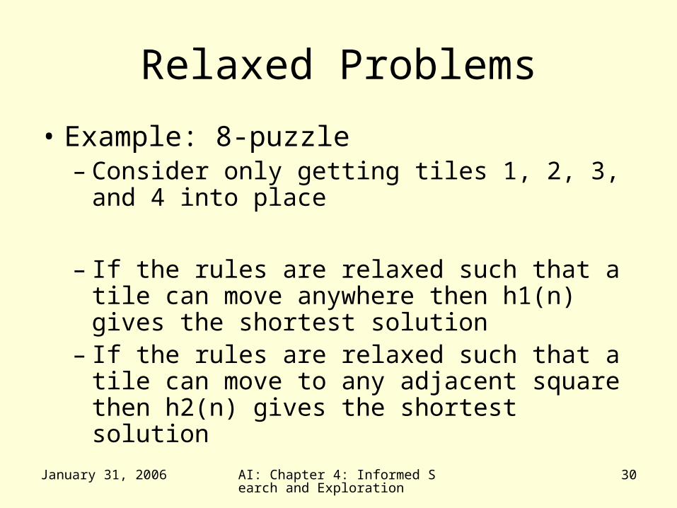
Relaxed Problems
• Example: 8-puzzle– Consider only getting tiles 1, 2, 3, and 4
into place
– If the rules are relaxed such that a tile can move anywhere then h1(n) gives the shortest solution
– If the rules are relaxed such that a tile can move to any adjacent square then h2(n) gives the shortest solution
January 31, 2006 AI: Chapter 4: Informed Search and Exploration
31
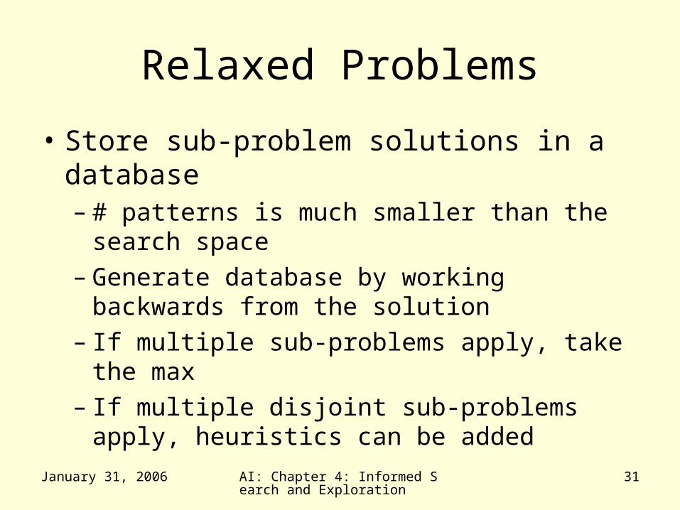
Relaxed Problems
• Store sub-problem solutions in a database– # patterns is much smaller than the
search space– Generate database by working backwards
from the solution– If multiple sub-problems apply, take the
max– If multiple disjoint sub-problems apply,
heuristics can be added
January 31, 2006 AI: Chapter 4: Informed Search and Exploration
32
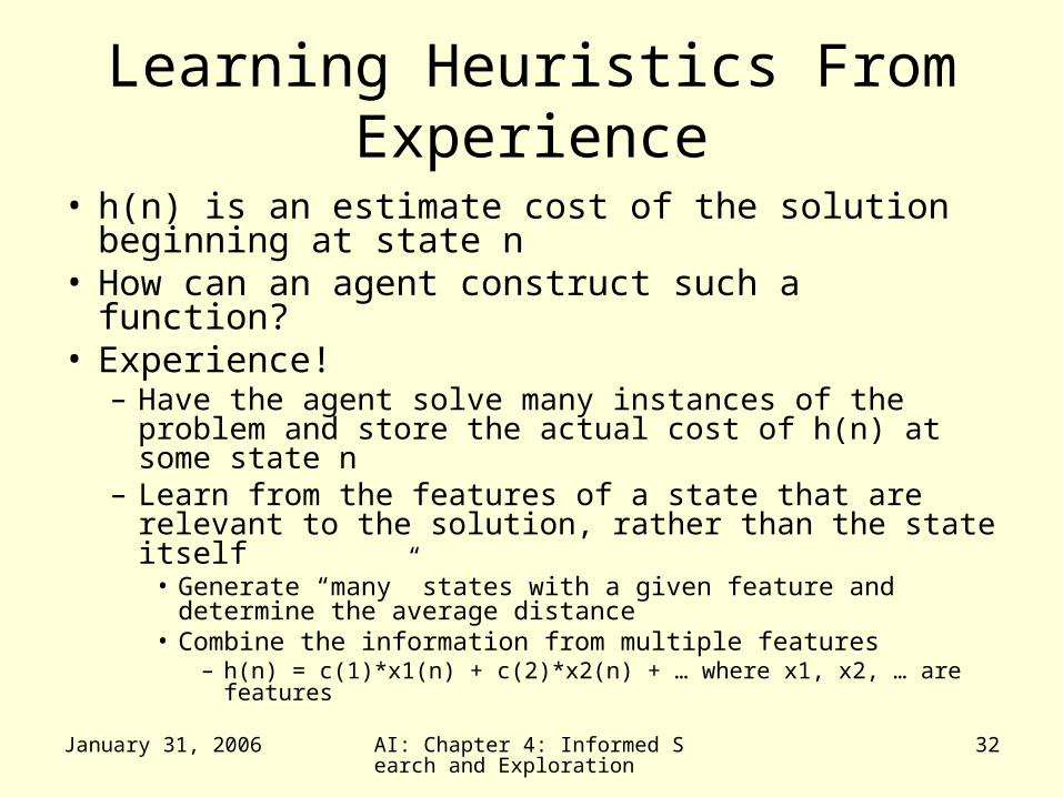
Learning Heuristics From Experience
• h(n) is an estimate cost of the solution beginning at state n
• How can an agent construct such a function?• Experience!
– Have the agent solve many instances of the problem and store the actual cost of h(n) at some state n
– Learn from the features of a state that are relevant to the solution, rather than the state itself
• Generate “many” states with a given feature and determine the average distance
• Combine the information from multiple features– h(n) = c(1)*x1(n) + c(2)*x2(n) + … where x1, x2, … are
features
January 31, 2006 AI: Chapter 4: Informed Search and Exploration
33
Optimization Problems
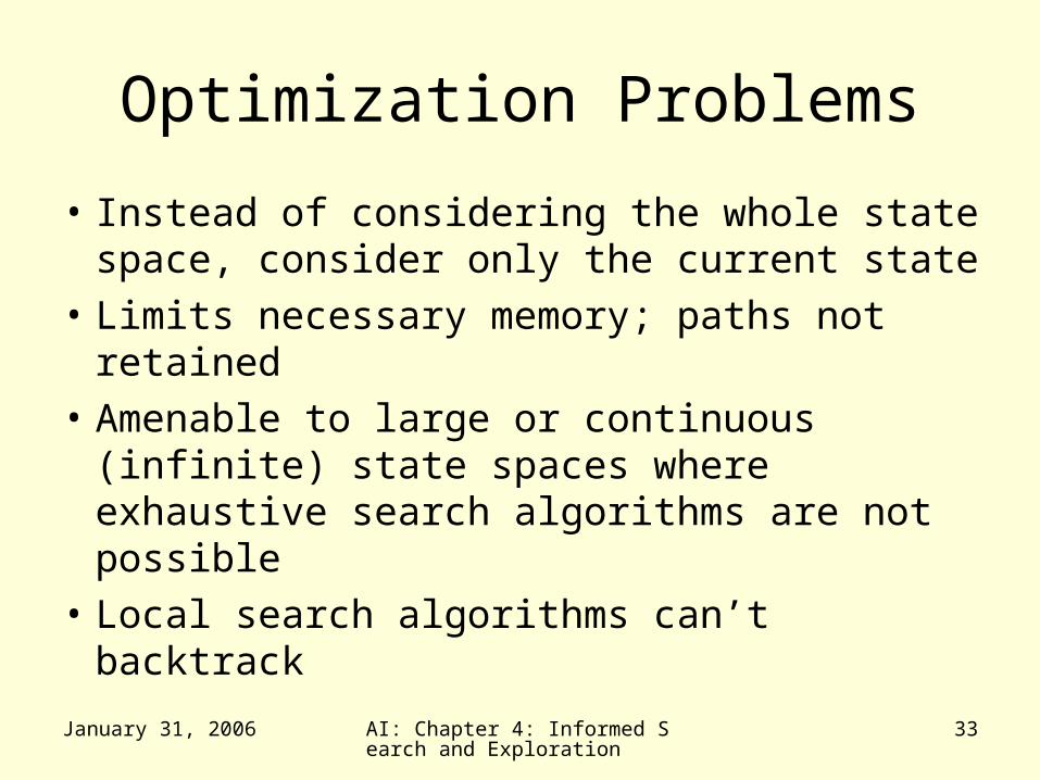
• Instead of considering the whole state space, consider only the current state
• Limits necessary memory; paths not retained
• Amenable to large or continuous (infinite) state spaces where exhaustive search algorithms are not possible
• Local search algorithms can’t backtrack
January 31, 2006 AI: Chapter 4: Informed Search and Exploration
34
Local Search Algorithms
• They are useful for solving optimization problems– Aim is to find a best state according to an
objective function
• Many optimization problems do not fit the standard search model outlined in chapter 3– E.g. There is no goal test or path cost in
Darwinian evolution
• State space landscape
January 31, 2006 AI: Chapter 4: Informed Search and Exploration
35
Optimization Problems
• Given measure of goodness (of fit)– Find optimal parameters (e.g correspondences)– That maximize goodness measure (or minimize
badness measure)
• Optimization techniques– Direct (closed-form)– Search (generate-test)– Heuristic search (e.g Hill Climbing)– Genetic Algorithm
January 31, 2006 AI: Chapter 4: Informed Search and Exploration
36
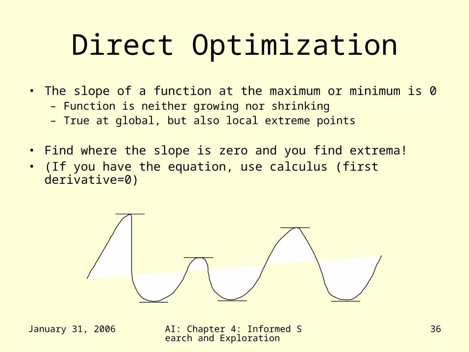
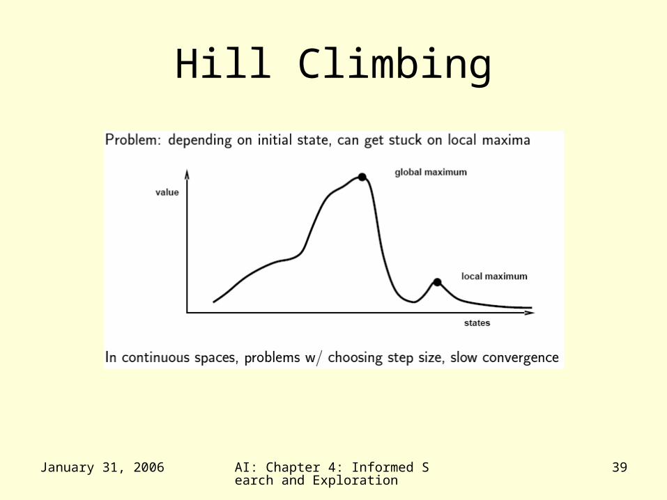
Direct Optimization• The slope of a function at the maximum or minimum is 0
– Function is neither growing nor shrinking– True at global, but also local extreme points
• Find where the slope is zero and you find extrema!• (If you have the equation, use calculus (first derivative=0)
January 31, 2006 AI: Chapter 4: Informed Search and Exploration
37
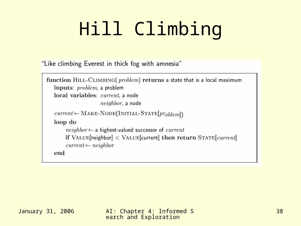
Hill Climbing
• Consider all possible successors as “one step” from the current state on the landscape.
• At each iteration, go to – The best successor (steepest ascent)– Any uphill move (first choice)– Any uphill move but steeper is more
probable (stochastic) • All variations get stuck at local
maxima
January 31, 2006 AI: Chapter 4: Informed Search and Exploration
38
Hill Climbing
January 31, 2006 AI: Chapter 4: Informed Search and Exploration
39
Hill Climbing
January 31, 2006 AI: Chapter 4: Informed Search and Exploration
40
Hill Climbing
• Local maxima = no uphill step– Algorithms on previous slide fail (not complete)– Allow “random restart” which is complete, but
might take a very long time
• Plateau = all steps equal (flat or shoulder)– Must move to equal state to make progress,
but no indication of the correct direction
• Ridge = narrow path of maxima, but might have to go down to go up (e.g. diagonal ridge in 4-direction space)
January 31, 2006 AI: Chapter 4: Informed Search and Exploration
41
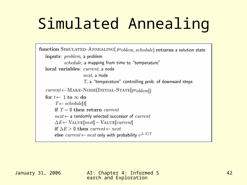
Simulated Annealing• Idea: Escape local maxima by allowing some
“bad” moves– But gradually decreasing their frequency
• Algorithm is randomized: – Take a step if random number is less than a value based
on both the objective function and the Temperature
• When Temperature is high, chance of going toward a higher value of optimization function J(x) is greater
• Note higher dimension: “perturb parameter vector” vs. “look at next and previous value”
January 31, 2006 AI: Chapter 4: Informed Search and Exploration
42
Simulated Annealing
January 31, 2006 AI: Chapter 4: Informed Search and Exploration
43
Genetic Algorithms
• Quicker but randomized searching for an optimal parameter vector
• Operations– Crossover (2 parents -> 2 children)– Mutation (one bit)
• Basic structure– Create population– Perform crossover & mutation (on fittest)– Keep only fittest children
January 31, 2006 AI: Chapter 4: Informed Search and Exploration
44
Genetic Algorithms
• Children carry parts of their parents’ data
• Only “good” parents can reproduce– Children are at least as “good” as parents?
• No, but “worse” children don’t last long
• Large population allows many “current points” in search– Can consider several regions (watersheds) at
once
January 31, 2006 AI: Chapter 4: Informed Search and Exploration
45
Genetic Algorithms
• Representation– Children (after crossover) should be similar to
parent, not random– Binary representation of numbers isn’t good -
what happens when you crossover in the middle of a number?
– Need “reasonable” breakpoints for crossover (e.g. between R, xcenter and ycenter but not within them)
• “Cover”– Population should be large enough to “cover” the
range of possibilities– Information shouldn’t be lost too soon – Mutation helps with this issue
January 31, 2006 AI: Chapter 4: Informed Search and Exploration
46
Experimenting With GAs
• Be sure you have a reasonable “goodness” criterion
• Choose a good representation (including methods for crossover and mutation)
• Generate a sufficiently random, large enough population
• Run the algorithm “long enough”• Find the “winners” among the population• Variations: multiple populations, keeping
vs. not keeping parents, “immigration / emigration”, mutation rate, etc.