4 INFORMED SEARCH AND EXPLORATION

4 INFORMED SEARCH ANDEXPLORATION

In which we see how information about the state space can prevent algorithmsfrom blundering about in the dark.

Chapter 3 showed that uninformed search strategies can find solutions to problems by system-atically generating new states and testing them against the goal. Unfortunately, these strate-gies are incredibly inefficient in most cases. This chapter shows how an informed searchstrategy—one that uses problem-specific knowledge—can find solutions more efficiently.Section 4.1 describes informed versions of the algorithms in Chapter 3, and Section 4.2 ex-plains how the necessary problem-specific information can be obtained. Sections 4.3 and 4.4cover algorithms that perform purely local search in the state space, evaluating and modify-ing one or more current states rather than systematically exploring paths from an initial state.These algorithms are suitable for problems in which the path cost is irrelevant and all thatmatters is the solution state itself. The family of local-search algorithms includes methodsinspired by statistical physics (simulated annealing) and evolutionary biology (genetic al-gorithms). Finally, Section 4.5 investigates online search, in which the agent is faced with astate space that is completely unknown.

4.1 INFORMED (HEURISTIC) SEARCH STRATEGIES

This section shows how an informed search strategy—one that uses problem-specific knowl-INFORMED SEARCH

edge beyond the definition of the problem itself—can find solutions more efficiently than anuninformed strategy.

The general approach we will consider is called best-first search. Best-first search isBEST-FIRST SEARCH

an instance of the general TREE-SEARCH or GRAPH-SEARCH algorithm in which a node isselected for expansion based on an evaluation function, f(n). Traditionally, the node withEVALUATION

FUNCTION

the lowest evaluation is selected for expansion, because the evaluation measures distance tothe goal. Best-first search can be implemented within our general search framework via apriority queue, a data structure that will maintain the fringe in ascending order of f -values.

The name “best-first search” is a venerable but inaccurate one. After all, if we couldreally expand the best node first, it would not be a search at all; it would be a straight march to

94

Section 4.1. Informed (Heuristic) Search Strategies 95

the goal. All we can do is choose the node that appears to be best according to the evaluationfunction. If the evaluation function is exactly accurate, then this will indeed be the bestnode; in reality, the evaluation function will sometimes be off, and can lead the search astray.Nevertheless, we will stick with the name “best-first search,” because “seemingly-best-firstsearch” is a little awkward.

There is a whole family of BEST-FIRST-SEARCH algorithms with different evaluationfunctions.1 A key component of these algorithms is a heuristic function,2 denoted h(n):HEURISTIC

FUNCTION

h(n) = estimated cost of the cheapest path from node n to a goal node.

For example, in Romania, one might estimate the cost of the cheapest path from Arad toBucharest via the straight-line distance from Arad to Bucharest.

Heuristic functions are the most common form in which additional knowledge of theproblem is imparted to the search algorithm. We will study heuristics in more depth in Sec-tion 4.2. For now, we will consider them to be arbitrary problem-specific functions, with oneconstraint: if n is a goal node, then h(n)= 0. The remainder of this section covers two waysto use heuristic information to guide search.

Greedy best-first search

Greedy best-first search3 tries to expand the node that is closest to the goal, on the groundsGREEDY BEST-FIRSTSEARCH

that this is likely to lead to a solution quickly. Thus, it evaluates nodes by using just theheuristic function: f(n) = h(n).

Let us see how this works for route-finding problems in Romania, using the straight-line distance heuristic, which we will call hSLD . If the goal is Bucharest, we will need toSTRAIGHT-LINE

DISTANCE

know the straight-line distances to Bucharest, which are shown in Figure 4.1. For example,hSLD(In(Arad))= 366. Notice that the values of hSLD cannot be computed from the prob-lem description itself. Moreover, it takes a certain amount of experience to know that hSLD

is correlated with actual road distances and is, therefore, a useful heuristic.

Urziceni

NeamtOradea

Zerind

Timisoara

Mehadia

Sibiu

PitestiRimnicu Vilcea

Vaslui

Bucharest

GiurgiuHirsova

Eforie

Arad

Lugoj

DobretaCraiova

Fagaras

Iasi

0160242161

77151

366

244226

176

241

25332980

199

380234

374

100193

Figure 4.1 Values of hSLD—straight-line distances to Bucharest.

1 Exercise 4.3 asks you to show that this family includes several familiar uninformed algorithms.2 A heuristic function h(n) takes a node as input, but is depends only on the state at that node.3 Our first edition called this greedy search; other authors have called it best-first search. Our more generalusage of the latter term follows Pearl (1984).

96 Chapter 4. Informed Search and Exploration

Rimnicu Vilcea

Zerind

Arad

Sibiu

Arad Fagaras Oradea

Timisoara

Sibiu Bucharest

329 374

366 380 193

253 0

Rimnicu Vilcea

Arad

Sibiu

Arad Fagaras Oradea

Timisoara

329

Zerind

374

366 176 380 193

Zerind

Arad

Sibiu Timisoara

253 329 374

Arad

366

(a) The initial state

(b) After expanding Arad

(c) After expanding Sibiu

(d) After expanding Fagaras

Figure 4.2 Stages in a greedy best-first search for Bucharest using the straight-line dis-tance heuristic hSLD . Nodes are labeled with their h-values.

Figure 4.2 shows the progress of a greedy best-first search using hSLD to find a pathfrom Arad to Bucharest. The first node to be expanded from Arad will be Sibiu, because itis closer to Bucharest than either Zerind or Timisoara. The next node to be expanded willbe Fagaras, because it is closest. Fagaras in turn generates Bucharest, which is the goal.For this particular problem, greedy best-first search using hSLD finds a solution without everexpanding a node that is not on the solution path; hence, its search cost is minimal. It isnot optimal, however: the path via Sibiu and Fagaras to Bucharest is 32 kilometers longerthan the path through Rimnicu Vilcea and Pitesti. This shows why the algorithm is called“greedy”—at each step it tries to get as close to the goal as it can.

Minimizing h(n) is susceptible to false starts. Consider the problem of getting fromIasi to Fagaras. The heuristic suggests that Neamt be expanded first, because it is closest


to Fagaras, but it is a dead end. The solution is to go first to Vaslui—a step that is actuallyfarther from the goal according to the heuristic—and then to continue to Urziceni, Bucharest,and Fagaras. In this case, then, the heuristic causes unnecessary nodes to be expanded. Fur-thermore, if we are not careful to detect repeated states, the solution will never be found—thesearch will oscillate between Neamt and Iasi.

Greedy best-first search resembles depth-first search in the way it prefers to follow asingle path all the way to the goal, but will back up when it hits a dead end. It suffers fromthe same defects as depth-first search—it is not optimal, and it is incomplete (because it canstart down an infinite path and never return to try other possibilities). The worst-case timeand space complexity is O(bm), where m is the maximum depth of the search space. With agood heuristic function, however, the complexity can be reduced substantially. The amountof the reduction depends on the particular problem and on the quality of the heuristic.

A* search: Minimizing the total estimated solution cost

The most widely-known form of best-first search is called A∗ search (pronounced “A-starA∗

SEARCH

search”). It evaluates nodes by combining g(n), the cost to reach the node, and h(n), the costto get from the node to the goal:

f(n) = g(n) + h(n) .

Since g(n) gives the path cost from the start node to node n, and h(n) is the estimated costof the cheapest path from n to the goal, we have

f(n) = estimated cost of the cheapest solution through n .

Thus, if we are trying to find the cheapest solution, a reasonable thing to try first is thenode with the lowest value of g(n) + h(n). It turns out that this strategy is more than justreasonable: provided that the heuristic function h(n) satisfies certain conditions, A∗ search isboth complete and optimal.

The optimality of A∗ is straightforward to analyze if it is used with TREE-SEARCH.In this case, A∗ is optimal if h(n) is an admissible heuristic—that is, provided that h(n)ADMISSIBLE

HEURISTIC

never overestimates the cost to reach the goal. Admissible heuristics are by nature optimistic,because they think the cost of solving the problem is less than it actually is. Since g(n) is theexact cost to reach n, we have as immediate consequence that f(n) never overestimates thetrue cost of a solution through n.

An obvious example of an admissible heuristic is the straight-line distance hSLD thatwe used in getting to Bucharest. Straight-line distance is admissible because the shortest pathbetween any two points is a straight line, so the straight line cannot be an overestimate. InFigure 4.3, we show the progress of an A∗ tree search for Bucharest. The values of g arecomputed from the step costs in Figure 3.2, and the values of hSLD are given in Figure 4.1.Notice in particular that Bucharest first appears on the fringe at step (e), but it is not selectedfor expansion because its f -cost (450) is higher than that of Pitesti (417). Another way tosay this is that there might be a solution through Pitesti whose cost is as low as 417, so thealgorithm will not settle for a solution that costs 450. From this example, we can extracta general proof that A∗ using TREE-SEARCH is optimal if h(n) is admissible. Suppose a


(a) The initial state

(b) After expanding Arad

(c) After expanding Sibiu

Arad

Sibiu Timisoara

447=118+329

Zerind

449=75+374393=140+253

Arad

366=0+366

(d) After expanding Rimnicu Vilcea

(e) After expanding Fagaras

(f) After expanding Pitesti

Zerind

Arad

Sibiu

Arad

Timisoara

Rimnicu VilceaFagaras Oradea

447=118+329 449=75+374

646=280+366 413=220+193415=239+176 671=291+380

Zerind

Arad

Sibiu Timisoara

447=118+329 449=75+374

Rimnicu Vilcea

Craiova Pitesti Sibiu

526=366+160 553=300+253417=317+100

Zerind

Arad

Sibiu

Arad

Timisoara

Sibiu Bucharest

Fagaras Oradea


447=118+329 449=75+374

646=280+366

591=338+253 450=450+0 526=366+160 553=300+253417=317+100

671=291+380

Zerind

Arad

Sibiu

Arad

Timisoara

Sibiu Bucharest

Oradea


Bucharest Craiova Rimnicu Vilcea

418=418+0

447=118+329 449=75+374

646=280+366

591=338+253 450=450+0 526=366+160 553=300+253

615=455+160 607=414+193

671=291+380

Rimnicu Vilcea

Fagaras Rimnicu Vilcea

Arad Fagaras Oradea

646=280+366 415=239+176 671=291+380

Figure 4.3 Stages in an A∗ search for Bucharest. Nodes are labeled with f = g + h. Theh values are the straight-line distances to Bucharest taken from Figure 4.1.


suboptimal goal node G2 appears on the fringe, and let the cost of the optimal solution be C∗.Then, because G2 is suboptimal and because h(G2)= 0 (true for any goal node), we know

f(G2) = g(G2) + h(G2) = g(G2) > C∗ .

Now consider a fringe node n that is on an optimal solution path—for example, Pitesti in theexample of the preceding paragraph. (There must always be such a node if a solution exists.)If h(n) does not overestimate the cost of completing the solution path, then we know that

f(n) = g(n) + h(n) ≤ C∗ .

Now we have shown that f(n) ≤ C∗ < f(G2), so G2 will not be expanded and A∗ mustreturn an optimal solution.

If we use the GRAPH-SEARCH algorithm of Figure 3.19 instead of TREE-SEARCH,then this proof breaks down. Suboptimal solutions can be returned because GRAPH-SEARCH

can discard the optimal path to a repeated state if it is not the first one generated. (SeeExercise 4.4.) There are two ways to fix this problem. The first solution is to extendGRAPH-SEARCH so that it discards the more expensive of any two paths found to the samenode. (See the discussion in Section 3.5.) The extra bookkeeping is messy, but it does guar-antee optimality. The second solution is to ensure that the optimal path to any repeated state isalways the first one followed—as is the case with uniform-cost search. This property holds ifwe impose an extra requirement on h(n), namely the requirement of consistency (also calledCONSISTENCY

monotonicity). A heuristic h(n) is consistent if, for every node n and every successor n′ ofMONOTONICITY

n generated by any action a, the estimated cost of reaching the goal from n is no greater thanthe step cost of getting to n′ plus the estimated cost of reaching the goal from n′:

h(n) ≤ c(n, a, n′) + h(n′) .

This is a form of the general triangle inequality, which stipulates that each side of a triangleTRIANGLEINEQUALITY

cannot be longer than the sum of the other two sides. Here, the triangle is formed by n, n′,and the goal closest to n. It is fairly easy to show (Exercise 4.7) that every consistent heuristicis also admissible. The most important consequence of consistency is the following: A∗ usingGRAPH-SEARCH is optimal if h(n) is consistent.

Although consistency is a stricter requirement than admissibility, one has to work quitehard to concoct heuristics that are admissible but not consistent. All the admissible heuristicswe discuss in this chapter are also consistent. Consider, for example, hSLD . We know thatthe general triangle inequality is satisfied when each side is measured by the straight-linedistance, and that the straight-line distance between n and n′ is no greater than c(n, a, n′).Hence, hSLD is a consistent heuristic.

Another important consequence of consistency is the following: If h(n) is consistent,then the values of f(n) along any path are nondecreasing. The proof follows directly fromthe definition of consistency. Suppose n′ is a successor of n; then g(n′)= g(n) + c(n, a, n′)for some a, and we have

f(n′) = g(n′) + h(n′) = g(n) + c(n, a, n′) + h(n′) ≥ g(n) + h(n) = f(n) .

It follows that the sequence of nodes expanded by A∗ using GRAPH-SEARCH is in nonde-creasing order of f(n). Hence, the first goal node selected for expansion must be an optimalsolution, since all later nodes will be at least as expensive.


O

Z

A

T

L

M

DC

R

F

P

G

BU

H

E

V

I

N

380

400

420

S

Figure 4.4 Map of Romania showing contours at f = 380, f = 400 and f = 420, withArad as the start state. Nodes inside a given contour have f -costs less than or equal to thecontour value.

The fact that f -costs are nondecreasing along any path also means that we can drawcontours in the state space, just like the contours in a topographic map. Figure 4.4 shows anCONTOURS

example. Inside the contour labeled 400, all nodes have f(n) less than or equal to 400, and soon. Then, because A∗ expands the fringe node of lowest f -cost, we can see that an A∗ searchfans out from the start node, adding nodes in concentric bands of increasing f -cost.

With uniform-cost search (A∗ search using h(n) = 0), the bands will be “circular”around the start state. With more accurate heuristics, the bands will stretch toward the goalstate and become more narrowly focused around the optimal path. If C∗ is the cost of theoptimal solution path, then we can say the following:

• A∗ expands all nodes with f(n) < C∗.

• A∗ might then expand some of the nodes right on the “goal contour” (where f(n) = C∗)before selecting a goal node.

Intuitively, it is obvious that the first solution found must be an optimal one, because goalnodes in all subsequent contours will have higher f -cost, and thus higher g-cost (because allgoal nodes have h(n) = 0). Intuitively, it is also obvious that A∗ search is complete. As weadd bands of increasing f , we must eventually reach a band where f is equal to the cost ofthe path to a goal state.4

Notice that A∗ expands no nodes with f(n) > C∗—for example, Timisoara is notexpanded in Figure 4.3 even though it is a child of the root. We say that the subtree belowTimisoara is pruned; because hSLD is admissible, the algorithm can safely ignore this subtreePRUNING

4 Completeness requires that there be only finitely many nodes with cost less than or equal to C∗, a condition

that is true if all step costs exceed some finite ε and if b is finite.


while still guaranteeing optimality. The concept of pruning—eliminating possibilities fromconsideration without having to examine them—is important for many areas of AI.

One final observation is that among optimal algorithms of this type—algorithms thatextend search paths from the root—A∗ is optimally efficient for any given heuristic function.OPTIMALLY

EFFICIENT

That is, no other optimal algorithm is guaranteed to expand fewer nodes than A∗ (exceptpossibly through tie-breaking among nodes with f(n)=C∗). This is because any algorithmthat does not expand all nodes with f(n) < C∗ runs the risk of missing the optimal solution.

That A∗ search is complete, optimal, and optimally efficient among all such algorithmsis rather satisfying. Unfortunately, it does not mean that A∗ is the answer to all our searchingneeds. The catch is that, for most problems, the number of nodes within the goal contoursearch space is still exponential in the length of the solution. Although the proof of the resultis beyond the scope of this book, it has been shown that exponential growth will occur unlessthe error in the heuristic function grows no faster than the logarithm of the actual path cost.In mathematical notation, the condition for subexponential growth is that

|h(n)− h∗(n)| ≤ O(log h∗(n)) ,

where h∗(n) is the true cost of getting from n to the goal. For almost all heuristics in practicaluse, the error is at least proportional to the path cost, and the resulting exponential growtheventually overtakes any computer. For this reason, it is often impractical to insist on findingan optimal solution. One can use variants of A∗ that find suboptimal solutions quickly, or onecan sometimes design heuristics that are more accurate, but not strictly admissible. In anycase, the use of a good heuristic still provides enormous savings compared to the use of anuninformed search. In Section 4.2, we will look at the question of designing good heuristics.

Computation time is not, however, A∗’s main drawback. Because it keeps all generatednodes in memory (as do all GRAPH-SEARCH algorithms), A∗ usually runs out of space longbefore it runs out of time. For this reason, A∗ is not practical for many large-scale prob-lems. Recently developed algorithms have overcome the space problem without sacrificingoptimality or completeness, at a small cost in execution time. These are discussed next.

Memory-bounded heuristic search

The simplest way to reduce memory requirements for A∗ is to adapt the idea of iterative deep-ening to the heuristic search context, resulting in the iterative-deepening A∗ (IDA∗) algorithm.The main difference between IDA∗ and standard iterative deepening is that the cutoff usedis the f -cost (g + h) rather than the depth; at each iteration, the cutoff value is the small-est f -cost of any node that exceeded the cutoff on the previous iteration. IDA∗ is practicalfor many problems with unit step costs and avoids the substantial overhead associated withkeeping a sorted queue of nodes. Unfortunately, it suffers from the same difficulties with real-valued costs as does the iterative version of uniform-cost search described in Exercise 3.11.This section briefly examines two more recent memory-bounded algorithms, called RBFSand MA∗.

Recursive best-first search (RBFS) is a simple recursive algorithm that attempts toRECURSIVEBEST-FIRST SEARCH

mimic the operation of standard best-first search, but using only linear space. The algorithm isshown in Figure 4.5. Its structure is similar to that of a recursive depth-first search, but rather


function RECURSIVE-BEST-FIRST-SEARCH(problem) returns a solution, or failureRBFS(problem , MAKE-NODE(INITIAL-STATE[problem]),∞)

function RBFS(problem ,node, f limit) returns a solution, or failure and a new f -cost limitif GOAL-TEST[problem](state) then return node

successors← EXPAND(node ,problem)if successors is empty then return failure ,∞for each s in successors do

f [s]←max(g(s) + h(s), f [node])repeat

best← the lowest f -value node in successors

if f [best ] > f limit then return failure , f [best]alternative← the second-lowest f -value among successors

result , f [best]←RBFS(problem , best , min( f limit , alternative))if result 6= failure then return result

Figure 4.5 The algorithm for recursive best-first search.

than continuing indefinitely down the current path, it keeps track of the f -value of the bestalternative path available from any ancestor of the current node. If the current node exceedsthis limit, the recursion unwinds back to the alternative path. As the recursion unwinds, RBFSreplaces the f -value of each node along the path with the best f -value of its children. In thisway, RBFS remembers the f -value of the best leaf in the forgotten subtree and can thereforedecide whether it’s worth reexpanding the subtree at some later time. Figure 4.6 shows howRBFS reaches Bucharest.

RBFS is somewhat more efficient than IDA∗, but still suffers from excessive node re-generation. In the example in Figure 4.6, RBFS first follows the path via Rimnicu Vilcea,then “changes its mind” and tries Fagaras, and then changes its mind back again. These mindchanges occur because every time the current best path is extended, there is a good chancethat its f -value will increase—h is usually less optimistic for nodes closer to the goal. Whenthis happens, particularly in large search spaces, the second-best path might become the bestpath, so the search has to backtrack to follow it. Each mind change corresponds to an iterationof IDA∗, and could require many reexpansions of forgotten nodes to recreate the best path andextend it one more node.

Like A∗, RBFS is an optimal algorithm if the heuristic function h(n) is admissible. Itsspace complexity is O(bd), but its time complexity is rather difficult to characterize: it de-pends both on the accuracy of the heuristic function and on how often the best path changes asnodes are expanded. Both IDA∗ and RBFS are subject to the potentially exponential increasein complexity associated with searching on graphs (see Section 3.5), because they cannotcheck for repeated states other than those on the current path. Thus, they may explore thesame state many times.

IDA∗ and RBFS suffer from using too little memory. Between iterations, IDA∗ retainsonly a single number: the current f -cost limit. RBFS retains more information in memory,


Zerind

Arad

Sibiu

Arad Fagaras Oradea

Craiova Sibiu

Bucharest Craiova Rimnicu Vilcea

Zerind

Arad

Sibiu

Arad

Sibiu Bucharest

Rimnicu VilceaOradea

Zerind

Arad

Sibiu

Arad

Timisoara

Timisoara

Timisoara

Fagaras Oradea Rimnicu Vilcea


646 415 526

526 553

646 526

450591

646 526

526 553

418 615 607

447 449

447

447 449

449

366

393

366

393

413

413 417415

366

393

415 450 417Rimnicu Vilcea

Fagaras

447

415

447

447

417

(a) After expanding Arad, Sibiu, and Rimnicu Vilcea

(c) After switching back to Rimnicu Vilcea and expanding Pitesti

(b) After unwinding back to Sibiu and expanding Fagaras

447

447

∞

∞

∞

417

417

Pitesti

Figure 4.6 Stages in an RBFS search for the shortest route to Bucharest. The f -limitvalue for each recursive call is shown on top of each current node. (a) The path via RimnicuVilcea is followed until the current best leaf (Pitesti) has a value that is worse than the bestalternative path (Fagaras). (b) The recursion unwinds and the best leaf value of the forgottensubtree (417) is backed up to Rimnicu Vilcea; then Fagaras is expanded, revealing a bestleaf value of 450. (c) The recursion unwinds and the best leaf value of the forgotten subtree(450) is backed up to Fagaras; then Rimnicu Vilcea is expanded. This time, because the bestalternative path (through Timisoara) costs at least 447, the expansion continues to Bucharest.

but it uses only O(bd) memory: even if more memory were avalable, RBFS has no way tomake use of it.

It seems sensible, therefore, to use all available memory. Two algorithms that do thisare MA∗ (memory-bounded A∗) and SMA∗ (simplified MA∗). We will describe SMA∗, whichMA*

SMA*


is—well—simpler. SMA∗ proceeds just like A∗, expanding the best leaf until memory is full.At this point, it cannot add a new node to the search tree without dropping an old one. SMA∗

always drops the worst leaf node—the one with the highest f -value. Like RBFS, SMA∗

then backs up the value of the forgotten node to its parent. In this way, the ancestor of aforgotten subtree knows the quality of the best path in that subtree. With this information,SMA∗ regenerates the subtree only when all other paths have been shown to look worse thanthe path it has forgotten. Another way of saying this is that, if all the descendants of a node nare forgotten, then we will not know which way to go from n, but we will still have an ideaof how worthwhile it is to go anywhere from n.

The complete algorithm is too complicated to reproduce here,5 but there is one subtletyworth mentioning. We said that SMA∗ expands the best leaf and deletes the worst leaf. Whatif all the leaf nodes have the same f -value? Then the algorithm might select the same nodefor deletion and expansion. SMA∗ solves this problem by expanding the newest best leaf anddeleting the oldest worst leaf. These can be the same node only if there is only one leaf; in thatcase, the current search tree must be a single path from root to leaf that fills all of memory.If the leaf is not a goal node, then even if it is on an optimal solution path, that solution isnot reachable with the available memory. Therefore, the node can be discarded exactly as ifit had no successors.

SMA∗ is complete if there is any reachable solution—that is, if d, the depth of theshallowest goal node, is less than the memory size (expressed in nodes). It is optimal if anyoptimal solution is reachable; otherwise it returns the best reachable solution. In practicalterms, SMA∗ might well be the best general-purpose algorithm for finding optimal solutions,particularly when the state space is a graph, step costs are not uniform, and node generationis expensive compared to the additional overhead of maintaining the open and closed lists.

On very hard problems, however, it will often be the case that SMA∗ is forced to switchback and forth continually between a set of candidate solution paths, only a small subset ofwhich can fit in memory. (This resembles the problem of thrashing in disk paging systems.)THRASHING

Then the extra time required for repeated regeneration of the same nodes means that problemsthat would be practically solvable by A∗, given unlimited memory, become intractable forSMA∗. That is to say, memory limitations can make a problem intractable from the point ofview of computation time. Although there is no theory to explain the tradeoff between timeand memory, it seems that this is an inescapable problem. The only way out is to drop theoptimality requirement.

Learning to search better

We have presented several fixed strategies—breadth-first, greedy best-first, and so on—thathave been designed by computer scientists. Could an agent learn how to search better? Theanswer is yes, and the method rests on an important concept called the metalevel state space.METALEVEL STATE

SPACE

Each state in a metalevel state space captures the internal (computational) state of a programthat is searching in an object-level state space such as Romania. For example, the internalOBJECT-LEVEL STATE

SPACE

state of the A∗ algorithm consists of the current search tree. Each action in the metalevel state

5 A rough sketch appeared in the first edition of this book.

Section 4.2. Heuristic Functions 105

space is a computation step that alters the internal state; for example, each computation stepin A∗ expands a leaf node and adds its successors to the tree. Thus, Figure 4.3, which showsa sequence of larger and larger search trees, can be seen as depicting a path in the metalevelstate space where each state on the path is an object-level search tree.

Now, the path in Figure 4.3 has five steps, including one step, the expansion of Fagaras,that is not especially helpful. For harder problems, there will be many such missteps, and ametalevel learning algorithm can learn from these experiences to avoid exploring unpromis-METALEVEL

LEARNING

ing subtrees. The techniques used for this kind of learning are described in Chapter 21. Thegoal of learning is to minimize the total cost of problem solving, trading off computationalexpense and path cost.

4.2 HEURISTIC FUNCTIONS

In this section, we will look at heuristics for the 8-puzzle, in order to shed light on the natureof heuristics in general.

The 8-puzzle was one of the earliest heuristic search problems. As mentioned in Sec-tion 3.2, the object of the puzzle is to slide the tiles horizontally or vertically into the emptyspace until the configuration matches the goal configuration (Figure 4.7).

2

Start State Goal State

1

3 4

6 7

5

1

2

3

4

6

7

8

5

8

Figure 4.7 A typical instance of the 8-puzzle. The solution is 26 steps long.

The average solution cost for a randomly generated 8-puzzle instance is about 22 steps.The branching factor is about 3. (When the empty tile is in the middle, there are four possiblemoves; when it is in a corner there are two; and when it is along an edge there are three.) Thismeans that an exhaustive search to depth 22 would look at about 322 ≈ 3.1× 1010 states. Bykeeping track of repeated states, we could cut this down by a factor of about 170,000, becausethere are only 9!/2 = 181, 440 distinct states that are reachable. (See Exercise 3.4.) This isa manageable number, but the corresponding number for the 15-puzzle is roughly 1013, sothe next order of business is to find a good heuristic function. If we want to find the shortestsolutions by using A∗, we need a heuristic function that never overestimates the number ofsteps to the goal. There is a long history of such heuristics for the 15-puzzle; here are twocommonly-used candidates:


• h1 = the number of misplaced tiles. For Figure 4.7, all of the eight tiles are out ofposition, so the start state would have h1 = 8. h1 is an admissible heuristic, because itis clear that any tile that is out of place must be moved at least once.

• h2 = the sum of the distances of the tiles from their goal positions. Because tilescannot move along diagonals, the distance we will count is the sum of the horizontaland vertical distances. This is sometimes called the city block distance or Manhattandistance. h2 is also admissible, because all any move can do is move one tile one stepMANHATTAN

DISTANCE

closer to the goal. Tiles 1 to 8 in the start state give a Manhattan distance of

h2 = 3 + 1 + 2 + 2 + 2 + 3 + 3 + 2 = 18 .

As we would hope, neither of these overestimates the true solution cost, which is 26.

The effect of heuristic accuracy on performance

One way to characterize the quality of a heuristic is the effective branching factor b∗. If theEFFECTIVEBRANCHING FACTOR

total number of nodes generated by A∗ for a particular problem is N , and the solution depthis d, then b∗ is the branching factor that a uniform tree of depth d would have to have in orderto contain N + 1 nodes. Thus,

N + 1 = 1 + b∗ + (b∗)2 + · · ·+ (b∗)d .

For example, if A∗ finds a solution at depth 5 using 52 nodes, then the effective branchingfactor is 1.92. The effective branching factor can vary across problem instances, but usuallyit is fairly constant for sufficiently hard problems. Therefore, experimental measurements ofb∗ on a small set of problems can provide a good guide to the heuristic’s overall usefulness.A well-designed heuristic would have a value of b∗ close to 1, allowing fairly large problemsto be solved.

To test the heuristic functions h1 and h2, we generated 1200 random problems withsolution lengths from 2 to 24 (100 for each even number) and solved them with iterativedeepening search and with A∗ tree search using both h1 and h2. Figure 4.8 gives the averagenumber of nodes expanded by each strategy and the effective branching factor. The resultssuggest that h2 is better than h1, and is far better than using iterative deepening search. On oursolutions with length 14, A∗ with h2 is 30,000 times more efficient than uninformed iterativedeepening search.

One might ask whether h2 is always better than h1. The answer is yes. It is easy to seefrom the definitions of the two heuristics that, for any node n, h2(n) ≥ h1(n). We thus saythat h2 dominates h1. Domination translates directly into efficiency: A∗ using h2 will neverDOMINATION

expand more nodes than A∗ using h1 (except possibly for some nodes with f(n)=C∗). Theargument is simple. Recall the observation on page 100 that every node with f(n) < C∗ willsurely be expanded. This is the same as saying that every node with h(n) < C∗ − g(n) willsurely be expanded. But because h2 is at least as big as h1 for all nodes, every node that issurely expanded by A∗ search with h2 will also surely be expanded with h1, and h1 mightalso cause other nodes to be expanded as well. Hence, it is always better to use a heuristicfunction with higher values, provided it does not overestimate and that the computation timefor the heuristic is not too large.


Search Cost Effective Branching Factor

d IDS A∗(h1) A∗(h2) IDS A∗(h1) A∗(h2)

2 10 6 6 2.45 1.79 1.794 112 13 12 2.87 1.48 1.456 680 20 18 2.73 1.34 1.308 6384 39 25 2.80 1.33 1.24

10 47127 93 39 2.79 1.38 1.2212 3644035 227 73 2.78 1.42 1.2414 – 539 113 – 1.44 1.2316 – 1301 211 – 1.45 1.2518 – 3056 363 – 1.46 1.2620 – 7276 676 – 1.47 1.2722 – 18094 1219 – 1.48 1.2824 – 39135 1641 – 1.48 1.26

Figure 4.8 Comparison of the search costs and effective branching factors for theITERATIVE-DEEPENING-SEARCH and A∗ algorithms with h1, h2. Data are averaged over100 instances of the 8-puzzle, for various solution lengths.

Inventing admissible heuristic functions

We have seen that both h1 (misplaced tiles) and h2 (Manhattan distance) are fairly goodheuristics for the 8-puzzle and that h2 is better. How might one have come up with h2? Is itpossible for a computer to invent such a heuristic mechanically?

h1 and h2 are estimates of the remaining path length for the 8-puzzle, but they arealso perfectly accurate path lengths for simplified versions of the puzzle. If the rules of thepuzzle were changed so that a tile could move anywhere, instead of just to the adjacent emptysquare, then h1 would give the exact number of steps in the shortest solution. Similarly, ifa tile could move one square in any direction, even onto an occupied square, then h2 wouldgive the exact number of steps in the shortest solution. A problem with fewer restrictions onthe actions is called a relaxed problem. The cost of an optimal solution to a relaxed problemRELAXED PROBLEM

is an admissible heuristic for the original problem. The heuristic is admissible becausethe optimal solution in the original problem is, by definition, also a solution in the relaxedproblem and therefore must be at least as expensive as the optimal solution in the relaxedproblem. Because the derived heuristic is an exact cost for the relaxed problem, it must obeythe triangle inequality and is therefore consistent (see page 99).

If a problem definition is written down in a formal language, it is possible to constructrelaxed problems automatically.6 For example, if the 8-puzzle actions are described as

A tile can move from square A to square B ifA is horizontally or vertically adjacent to B and B is blank,

6 In Chapters 8 and 11, we will describe formal languages suitable for this task; with formal descriptions thatcan be manipulated, the construction of relaxed problems can be automated. For now, we will use English.


we can generate three relaxed problems by removing one or both of the conditions:

(a) A tile can move from square A to square B if A is adjacent to B.(b) A tile can move from square A to square B if B is blank.(c) A tile can move from square A to square B.

From (a), we can derive h2 (Manhattan distance). The reasoning is that h2 would be theproper score if we moved each tile in turn to its destination. The heuristic derived from (b) isdiscussed in Exercise 4.9. From (c), we can derive h1 (misplaced tiles), because it would bethe proper score if tiles could move to their intended destination in one step. Notice that it iscrucial that the relaxed problems generated by this technique can be solved essentially withoutsearch, because the relaxed rules allow the problem to be decomposed into eight independentsubproblems. If the relaxed problem is hard to solve, then the values of the correspondingheuristic will be expensive to obtain.7

A program called ABSOLVER can generate heuristics automatically from problem def-initions, using the “relaxed problem” method and various other techniques (Prieditis, 1993).ABSOLVER generated a new heuristic for the 8-puzzle better than any preexisting heuristicand found the first useful heuristic for the famous Rubik’s cube puzzle.

One problem with generating new heuristic functions is that one often fails to get one“clearly best” heuristic. If a collection of admissible heuristics h1 . . . hm is available for aproblem, and none of them dominates any of the others, which should we choose? As it turnsout, we need not make a choice. We can have the best of all worlds, by defining

h(n) = max{h1(n), . . . , hm(n)} .

This composite heuristic uses whichever function is most accurate on the node in question.Because the component heuristics are admissible, h is admissible; it is also easy to prove thath is consistent. Furthermore, h dominates all of its component heuristics.

Admissible heuristics can also be derived from the solution cost of a subproblem ofSUBPROBLEM

a given problem. For example, Figure 4.9 shows a subproblem of the 8-puzzle instancein Figure 4.7. The subproblem involves getting tiles 1, 2, 3, 4 into their correct positions.Clearly, the cost of the optimal solution of this subproblem is a lower bound on the cost ofthe complete problem. It turns out to be substantially more accurate than Manhattan distancein some cases.

The idea behind pattern databases is to store these exact solution costs for every pos-PATTERN DATABASES

sible subproblem instance—in our example, every possible configuration of the four tiles andthe blank. (Notice that the locations of the other four tiles are irrelevant for the purposes ofsolving the subproblem, but moves of those tiles do count towards the cost.) Then, we com-pute an admissible heuristic hDB for each complete state encountered during a search simplyby looking up the corresponding subproblem configuration in the database. The databaseitself is constructed by searching backwards from the goal state and recording the cost ofeach new pattern encountered; the expense of this search is amortized over many subsequentproblem instances.

7 Note that a perfect heuristic can be obtained simply by allowing h to run a full breadth-first search “on thesly.” Thus, there is a tradeoff between accuracy and computation time for heuristic functions.


Start State Goal State

1

2

3

4

6

8

5

21

3 6

7 8

54

Figure 4.9 A subproblem of the 8-puzzle instance given in Figure 4.7. The task is to gettiles 1, 2, 3, and 4 into their correct positions, without worrying about what happens to theother tiles.

The choice of 1-2-3-4 is fairly arbitrary; we could also construct databases for 5-6-7-8,and for 2-4-6-8, and so on. Each database yields an admissible heuristic, and these heuristicscan be combined, as explained earlier, by taking the maximum value. A combined heuristic ofthis kind is much more accurate than the Manhattan distance; the number of nodes generatedwhen solving random 15-puzzles can be reduced by a factor of 1000.

One might wonder whether the heuristics obtained from the 1-2-3-4 database and the5-6-7-8 could be added, since the two subproblems seem not to overlap. Would this still givean admissible heuristic? The answer is no, because the solutions of the 1-2-3-4 subproblemand the 5-6-7-8 subproblem for a given state will almost certainly share some moves—it isunlikely that 1-2-3-4 can be moved into place without touching 5-6-7-8, and vice versa. Butwhat if we don’t count those moves? That is, we record not the total cost of solving the1-2-3-4 subproblem, but just the number of moves involving 1-2-3-4. Then it is easy to seethat the sum of the two costs is still a lower bound on the cost of solving the entire problem.This is the idea behind disjoint pattern databases. Using such databases, it is possible toDISJOINT PATTERN

DATABASES

solve random 15-puzzles in a few milliseconds—the number of nodes generated is reducedby a factor of 10,000 compared with using Manhattan distance. For 24-puzzles, a speedup ofroughly a million can be obtained.

Disjoint pattern databases work for sliding-tile puzzles because the problem can bedivided up in such a way that each move affects only one subproblem—because only one tileis moved at a time. For a problem such as Rubik’s cube, this kind of subdivision cannot bedone because each move affects 8 or 9 of the 26 cubies. Currently, it is not clear how to definedisjoint databases for such problems.

Learning heuristics from experience

A heuristic function h(n) is supposed to estimate the cost of a solution beginning from thestate at node n. How could an agent construct such a function? One solution was given in thepreceding section—namely, to devise relaxed problems for which an optimal solution can befound easily. Another solution is to learn from experience. “Experience” here means solvinglots of 8-puzzles, for instance. Each optimal solution to an 8-puzzle problem provides ex-


amples from which h(n) can be learned. Each example consists of a state from the solutionpath and the actual cost of the solution from that point. From these examples, an inductivelearning algorithm can be used to construct a function h(n) that can (with luck) predict solu-tion costs for other states that arise during search. Techniques for doing just this using neuralnets, decision trees, and other methods are demonstrated in Chapter 18. (The reinforcementlearning methods described in Chapter 21 are also applicable.)

Inductive learning methods work best when supplied with features of a state that areFEATURES

relevant to its evaluation, rather than with just the raw state description. For example, thefeature “number of misplaced tiles” might be helpful in predicting the actual distance of astate from the goal. Let’s call this feature x1(n). We could take 100 randomly generated8-puzzle configurations and gather statistics on their actual solution costs. We might find thatwhen x1(n) is 5, the average solution cost is around 14, and so on. Given these data, thevalue of x1 can be used to predict h(n). Of course, we can use several features. A secondfeature x2(n) might be “number of pairs of adjacent tiles that are also adjacent in the goalstate.” How should x1(n) and x2(n) be combined to predict h(n)? A common approach isto use a linear combination:

h(n) = c1x1(n) + c2x2(n) .

The constants c1 and c2 are adjusted to give the best fit to the actual data on solution costs.Presumably, c1 should be positive and c2 should be negative.

4.3 LOCAL SEARCH ALGORITHMS AND OPTIMIZATION PROBLEMS

The search algorithms that we have seen so far are designed to explore search spaces sys-tematically. This systematicity is achieved by keeping one or more paths in memory and byrecording which alternatives have been explored at each point along the path and which havenot. When a goal is found, the path to that goal also constitutes a solution to the problem.

In many problems, however, the path to the goal is irrelevant. For example, in the 8-queens problem (see page 66), what matters is the final configuration of queens, not the orderin which they are added. This class of problems includes many important applications such asintegrated-circuit design, factory-floor layout, job-shop scheduling, automatic programming,telecommunications network optimization, vehicle routing, and portfolio management.

If the path to the goal does not matter, we might consider a different class of algo-rithms, ones that do not worry about paths at all. Local search algorithms operate usingLOCAL SEARCH

a single current state (rather than multiple paths) and generally move only to neighborsCURRENT STATE

of that state. Typically, the paths followed by the search are not retained. Although localsearch algorithms are not systematic, they have two key advantages: (1) they use very littlememory—usually a constant amount; and (2) they can often find reasonable solutions in largeor infinite (continuous) state spaces for which systematic algorithms are unsuitable.

In addition to finding goals, local search algorithms are useful for solving pure op-timization problems, in which the aim is to find the best state according to an objectiveOPTIMIZATION

PROBLEMS

function. Many optimization problems do not fit the “standard” search model introduced inOBJECTIVEFUNCTION

Section 4.3. Local Search Algorithms and Optimization Problems 111

Chapter 3. For example, nature provides an objective function—reproductive fitness—thatDarwinian evolution could be seen as attempting to optimize, but there is no “goal test” andno “path cost” for this problem.

To understand local search, we will find it very useful to consider the state space land-scape (as in Figure 4.10). A landscape has both “location” (defined by the state) and “eleva-STATE SPACE

LANDSCAPE

tion” (defined by the value of the heuristic cost function or objective function). If elevationcorresponds to cost, then the aim is to find the lowest valley—a global minimum; if eleva-GLOBAL MINIMUM

tion corresponds to an objective function, then the aim is to find the highest peak—a globalmaximum. (You can convert from one to the other just by inserting a minus sign.) LocalGLOBAL MAXIMUM

search algorithms explore this landscape. A complete local search algorithm always finds agoal if one exists; an optimal algorithm always finds a global minimum/maximum.

currentstate

objective function

state space

global maximum

local maximum

“flat” local maximum

shoulder

Figure 4.10 A one-dimensional state space landscape in which elevation corresponds tothe objective function. The aim is to find the global maximum. Hill-climbing search modifiesthe current state to try to improve it, as shown by the arrow. The various topographic featuresare defined in the text.

Hill-climbing search

The hill-climbing search algorithm is shown in Figure 4.11. It is simply a loop that continu-HILL-CLIMBING

ally moves in the direction of increasing value—that is, uphill. It terminates when it reaches a“peak” where no neighbor has a higher value. The algorithm does not maintain a search tree,so the current node data structure need only record the state and its objective function value.Hill-climbing does not look ahead beyond the immediate neighbors of the current state. Thisresembles trying to find the top of Mount Everest in a thick fog while suffering from amnesia.

To illustrate hill-climbing, we will use the 8-queens problem introduced on page 66.Local-search algorithms typically use a complete-state formulation, where each state has8 queens on the board, one per column. The successor function returns all possible statesgenerated by moving a single queen to another square in the same column (so each state has


function HILL-CLIMBING(problem) returns a state that is a local maximuminputs: problem , a problemlocal variables: current , a node

neighbor , a node

current←MAKE-NODE(INITIAL-STATE[problem])loop do

neighbor← a highest-valued successor of current

if VALUE[neighbor] ≤ VALUE[current] then return STATE[current ]current←neighbor

Figure 4.11 The hill-climbing search algorithm (steepest ascent version), which is themost basic local search technique. At each step the current node is replaced by the bestneighbor; in this version, that means the neighbor with the highest VALUE, but if a heuristiccost estimate h is used, we would find the neighbor with the lowest h.

14

18

17

15

14

18

14

14

14

14

14

12

16

12

13

16

17

14

18

13

14

17

15

18

15

13

15

13

12

15

15

13

15

12

13

14

14

14

16

12

14

12

12

15

16

13

14

12

14

18

16

16

16

14

16

14

(a) (b)

Figure 4.12 (a) An 8-queens state with heuristic cost estimate h =17, showing the valueof h for each possible successor obtained by moving a queen within its column. The bestmoves are marked. (b) A local minimum in the 8-queens state space; the state has h =1 butevery successor has a higher cost.

8× 7= 56 successors). The heuristic cost function h is the number of pairs of queens thatare attacking each other, either directly or indirectly. The global minimum of this functionis zero, which occurs only at perfect solutions. Figure 4.12(a) shows a state with h= 17.The figure also shows the values of all its successors, with the best successors having h= 12.Hill-climbing algorithms typically choose randomly among the set of best successors, if thereis more than one.


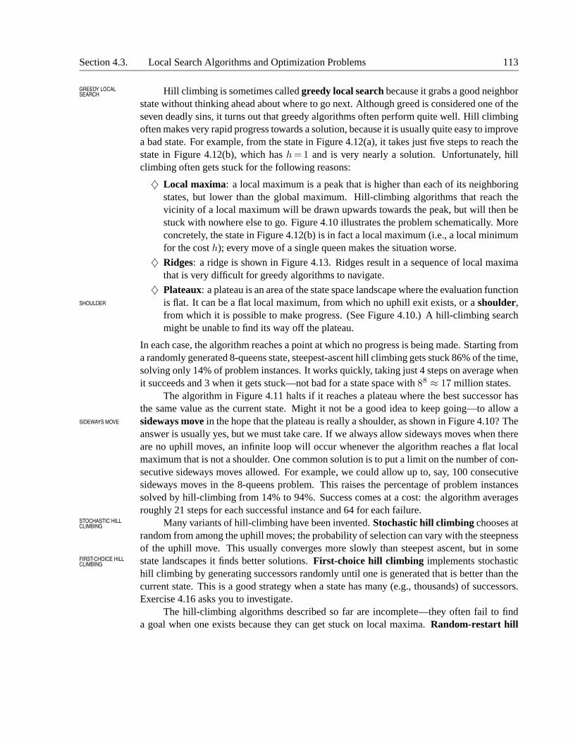
Hill climbing is sometimes called greedy local search because it grabs a good neighborGREEDY LOCALSEARCH

state without thinking ahead about where to go next. Although greed is considered one of theseven deadly sins, it turns out that greedy algorithms often perform quite well. Hill climbingoften makes very rapid progress towards a solution, because it is usually quite easy to improvea bad state. For example, from the state in Figure 4.12(a), it takes just five steps to reach thestate in Figure 4.12(b), which has h= 1 and is very nearly a solution. Unfortunately, hillclimbing often gets stuck for the following reasons:

♦ Local maxima: a local maximum is a peak that is higher than each of its neighboringstates, but lower than the global maximum. Hill-climbing algorithms that reach thevicinity of a local maximum will be drawn upwards towards the peak, but will then bestuck with nowhere else to go. Figure 4.10 illustrates the problem schematically. Moreconcretely, the state in Figure 4.12(b) is in fact a local maximum (i.e., a local minimumfor the cost h); every move of a single queen makes the situation worse.

♦ Ridges: a ridge is shown in Figure 4.13. Ridges result in a sequence of local maximathat is very difficult for greedy algorithms to navigate.

♦ Plateaux: a plateau is an area of the state space landscape where the evaluation functionis flat. It can be a flat local maximum, from which no uphill exit exists, or a shoulder,SHOULDER

from which it is possible to make progress. (See Figure 4.10.) A hill-climbing searchmight be unable to find its way off the plateau.

In each case, the algorithm reaches a point at which no progress is being made. Starting froma randomly generated 8-queens state, steepest-ascent hill climbing gets stuck 86% of the time,solving only 14% of problem instances. It works quickly, taking just 4 steps on average whenit succeeds and 3 when it gets stuck—not bad for a state space with 88 ≈ 17 million states.

The algorithm in Figure 4.11 halts if it reaches a plateau where the best successor hasthe same value as the current state. Might it not be a good idea to keep going—to allow asideways move in the hope that the plateau is really a shoulder, as shown in Figure 4.10? TheSIDEWAYS MOVE

answer is usually yes, but we must take care. If we always allow sideways moves when thereare no uphill moves, an infinite loop will occur whenever the algorithm reaches a flat localmaximum that is not a shoulder. One common solution is to put a limit on the number of con-secutive sideways moves allowed. For example, we could allow up to, say, 100 consecutivesideways moves in the 8-queens problem. This raises the percentage of problem instancessolved by hill-climbing from 14% to 94%. Success comes at a cost: the algorithm averagesroughly 21 steps for each successful instance and 64 for each failure.

Many variants of hill-climbing have been invented. Stochastic hill climbing chooses atSTOCHASTIC HILLCLIMBING

random from among the uphill moves; the probability of selection can vary with the steepnessof the uphill move. This usually converges more slowly than steepest ascent, but in somestate landscapes it finds better solutions. First-choice hill climbing implements stochasticFIRST-CHOICE HILL

CLIMBING

hill climbing by generating successors randomly until one is generated that is better than thecurrent state. This is a good strategy when a state has many (e.g., thousands) of successors.Exercise 4.16 asks you to investigate.

The hill-climbing algorithms described so far are incomplete—they often fail to finda goal when one exists because they can get stuck on local maxima. Random-restart hill


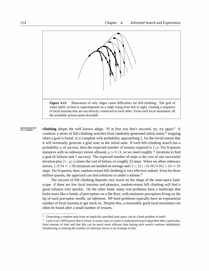
Figure 4.13 Illustration of why ridges cause difficulties for hill-climbing. The grid ofstates (dark circles) is superimposed on a ridge rising from left to right, creating a sequenceof local maxima that are not directly connected to each other. From each local maximum, allthe available actions point downhill.

climbing adopts the well known adage, “If at first you don’t succeed, try, try again.” ItRANDOM-RESTARTHILL CLIMBING

conducts a series of hill-climbing searches from randomly generated initial states,8 stoppingwhen a goal is found. It is complete with probability approaching 1, for the trivial reason thatit will eventually generate a goal state as the initial state. If each hill-climbing search has aprobability p of success, then the expected number of restarts required is 1/p. For 8-queensinstances with no sideways moves allowed, p ≈ 0.14, so we need roughly 7 iterations to finda goal (6 failures and 1 success). The expected number of steps is the cost of one successfuliteration plus (1−p)/p times the cost of failure, or roughly 22 steps. When we allow sidewaysmoves, 1/0.94 ≈ 1.06 iterations are needed on average and (1× 21)+(0.06/0.94)× 64 ≈ 25steps. For 8-queens, then, random-restart hill climbing is very effective indeed. Even for threemillion queens, the approach can find solutions in under a minute.9

The success of hill climbing depends very much on the shape of the state-space land-scape: if there are few local maxima and plateaux, random-restart hill climbing will find agood solution very quickly. On the other hand, many real problems have a landscape thatlooks more like a family of porcupines on a flat floor, with miniature porcupines living on thetip of each porcupine needle, ad infinitum. NP-hard problems typically have an exponentialnumber of local maxima to get stuck on. Despite this, a reasonably good local maximum canoften be found after a small number of restarts.

8 Generating a random state from an implicitly specified state space can be a hard problem in itself.9 Luby et al. (1993) prove that it is best, in some cases, to restart a randomized search algorithm after a particular,fixed amount of time and that this can be much more efficient than letting each search continue indefinitely.Disallowing or limiting the number of sideways moves is an example of this.


Simulated annealing search

A hill-climbing algorithm that never makes “downhill” moves towards states with lower value(or higher cost) is guaranteed to be incomplete, because it can get stuck on a local maximum.In contrast, a purely random walk—that is, moving to a successor chosen uniformly at ran-dom from the set of successors—is complete, but extremely inefficient. Therefore, it seemsreasonable to try to combine hill climbing with a random walk in some way that yields bothefficiency and completeness. Simulated annealing is such an algorithm. In metallurgy, an-SIMULATED

ANNEALING

nealing is the process used to temper or harden metals and glass by heating them to a hightemperature and then gradually cooling them, thus allowing the material to coalesce into alow-energy crystalline state. To understand simulated annealing, let’s switch our point ofview from hill climbing to gradient descent (i.e., minimizing cost) and imagine the task ofGRADIENT DESCENT

getting a ping-pong ball into the deepest crevice in a bumpy surface. If we just let the ballroll, it will come to rest at a local minimum. If we shake the surface, we can bounce the ballout of the local minimum. The trick is to shake just hard enough to bounce the ball out oflocal minima, but not hard enough to dislodge it from the global minimum. The simulated-annealing solution is to start by shaking hard (i.e., at a high temperature) and then graduallyreduce the intensity of the shaking (i.e., lower the temperature).

The innermost loop of the simulated-annealing algorithm (Figure 4.14) is quite similarto hill climbing. Instead of picking the best move, however, it picks a random move. If themove improves the situation, it is always accepted. Otherwise, the algorithm accepts the movewith some probability less than 1. The probability decreases exponentially with the “badness”of the move—the amount ∆E by which the evaluation is worsened. The probability alsodecreases as the “temperature” T goes down: “bad” moves are more likely to be allowed atthe start when temperature is high, and they become more unlikely as T decreases. One canprove that if the schedule lowers T slowly enough, the algorithm will find a global optimumwith probability approaching 1.

Simulated annealing was first used extensively to solve VLSI layout problems in theearly 1980s. It has been applied widely to factory scheduling and other large-scale optimiza-tion tasks. In Exercise 4.16, you are asked to compare its performance to that of random-restart hill climbing on the n-queens puzzle.

Local beam search

Keeping just one node in memory might seem to be an extreme reaction to the problem ofmemory limitations. The local beam search algorithm10 keeps track of k states rather thanLOCAL BEAM

SEARCH

just one. It begins with k randomly generated states. At each step, all the successors of all kstates are generated. If any one is a goal, the algorithm halts. Otherwise, it selects the k bestsuccessors from the complete list and repeats.

At first sight, a local beam search with k states might seem to be nothing more thanrunning k random restarts in parallel instead of in sequence. In fact, the two algorithmsare quite different. In a random-restart search, each search process runs independently of

10 Local beam search is an adaptation of beam search, which is a path-based algorithm.


function SIMULATED-ANNEALING(problem , schedule) returns a solution stateinputs: problem , a problem

schedule , a mapping from time to “temperature”local variables: current , a node

next , a nodeT , a “temperature” controlling the probability of downward steps

current←MAKE-NODE(INITIAL-STATE[problem])for t← 1 to∞ do

T ← schedule[t]if T = 0 then return current

next← a randomly selected successor of current

∆E←VALUE[next ] – VALUE[current ]if ∆E > 0 then current← next

else current← next only with probability e∆E/T

Figure 4.14 The simulated annealing search algorithm, a version of stochastic hill climb-ing where some downhill moves are allowed. Downhill moves are accepted readily early inthe annealing schedule and then less often as time goes on. The schedule input determinesthe value of T as a function of time.

the others. In a local beam search, useful information is passed among the k parallel searchthreads. For example, if one state generates several good successors and the other k−1 statesall generate bad successors, then the effect is that the first state says to the others, “Come overhere, the grass is greener!” The algorithm quickly abandons unfruitful searches and movesits resources to where the most progress is being made.

In its simplest form, local beam search can suffer from a lack of diversity among thek states—they can quickly become concentrated in a small region of the state space, makingthe search little more than an expensive version of hill climbing. A variant called stochasticbeam search, analogous to stochastic hill climbing, helps to alleviate this problem. InsteadSTOCHASTIC BEAM

SEARCH

of choosing the best k from the the pool of candidate successors, stochastic beam searchchooses k successors at random, with the probability of choosing a given successor beingan increasing function of its value. Stochastic beam search bears some resemblance to theprocess of natural selection, whereby the “successors” (offspring) of a “state” (organism)populate the next generation according to its “value” (fitness).

Genetic algorithms

A genetic algorithm (or GA) is a variant of stochastic beam search in which successor statesGENETICALGORITHM

are generated by combining two parent states, rather than by modifying a single state. Theanalogy to natural selection is the same as in stochastic beam search, except now we aredealing with sexual rather than asexual reproduction.

Like beam search, GAs begin with a set of k randomly generated states, called thepopulation. Each state, or individual, is represented as a string over a finite alphabet—mostPOPULATION

INDIVIDUAL


(a)

Initial Population

(b)

Fitness Function

(c)

Selection

(d)

Crossover

(e)

Mutation

24

23

20

11

29%

31%

26%

14%

32752411

24748552

32752411

24415124

32748552

24752411

32752124

24415411

32252124

24752411

32748152

24415417

24748552

32752411

24415124

32543213

Figure 4.15 The genetic algorithm. The initial population in (a) is ranked by the fitnessfunction in (b), resulting in pairs for mating in (c). They produce offspring in (d), which aresubject to mutation in (e).

+ =

Figure 4.16 The 8-queens states corresponding to the first two parents in Figure 4.15(c)and the first offspring in Figure 4.15(d). The shaded columns are lost in the crossover stepand the unshaded columns are retained.

commonly, a string of 0s and 1s. For example, an 8-queens state must specify the positions of8 queens, each in a column of 8 squares, and so requires 8× log2 8= 24 bits. Alternatively,the state could be represented as 8 digits, each in the range from 1 to 8. (We will see laterthat the two encodings behave differently.) Figure 4.15(a) shows a population of four 8-digitstrings representing 8-queens states.

The production of the next generation of states is shown in Figure 4.15(b)–(e). In (b),each state is rated by the evaluation function or (in GA terminology) the fitness function.FITNESS FUNCTION

A fitness function should return higher values for better states, so, for the 8-queens problemwe use the number of nonattacking pairs of queens, which has a value of 28 for a solution.The values of the four states are 24, 23, 20, and 11. In this particular variant of the geneticalgorithm, the probability of being chosen for reproducing is directly proportional to thefitness score, and the percentages are shown next to the raw scores.

In (c), a random choice of two pairs is selected for reproduction, in accordance with theprobabilities in (b). Notice that one individual is selected twice and one not at all.11 For each

11 There are many variants of this selection rule. The method of culling, in which all individuals below a giventhreshold are discarded, can be shown to converge faster than the random version (Baum et al., 1995).


pair to be mated, a crossover point is randomly chosen from the positions in the string. InCROSSOVER

Figure 4.15 the crossover points are after the third digit in the first pair and after the fifth digitin the second pair.12

In (d), the offspring themselves are created by crossing over the parent strings at thecrossover point. For example, the first child of the first pair gets the first three digits from thefirst parent and the remaining digits from the second parent, whereas the second child getsthe first three digits from the second parent and the rest from the first parent. The 8-queensstates involved in this reproduction step are shown in Figure 4.16. The example illustratesthe fact that, when two parent states are quite different, the crossover operation can producea state that is a long way from either parent state. It is often the case that the population isquite diverse early on in the process, so crossover (like simulated annealing) frequently takeslarge steps in the state space early in the search process and smaller steps later on when mostindividuals are quite similar.

Finally, in (e), each location is subject to random mutation with a small independentMUTATION

probability. One digit was mutated in the first, third, and fourth offspring. In the 8-queensproblem, this corresponds to choosing a queen at random and moving it to a random squarein its column. Figure 4.17 describes an algorithm that implements all these steps.

Like stochastic beam search, genetic algorithms combine an uphill tendency with ran-dom exploration and exchange of information among parallel search threads. The primaryadvantage, if any, of genetic algorithms comes from the crossover operation. Yet it can beshown mathematically that, if the positions of the genetic code is permuted initially in a ran-dom order, crossover conveys no advantage. Intuitively, the advantage comes from the abilityof crossover to combine large blocks of letters that have evolved independently to performuseful functions, thus raising the level of granularity at which the search operates. For ex-ample, it could be that putting the first three queens in positions 2, 4, and 6 (where they donot attack each other) constitutes a useful block that can be combined with other blocks toconstruct a solution.

The theory of genetic algorithms explains how this works using the idea of a schema,SCHEMA

which is a substring in which some of the positions can be left unspecified. For example,the schema 246***** describes all 8-queens states in which the first three queens are inpositions 2, 4, and 6 respectively. Strings that match the schema (such as 24613578) arecalled instances of the schema. It can be shown that, if the average fitness of the instances ofa schema is above the mean, then the number of instances of the schema within the populationwill grow over time. Clearly, this effect is unlikely to be significant if adjacent bits are totallyunrelated to each other, because then there will be few contiguous blocks that provide aconsistent benefit. Genetic algorithms work best when schemas correspond to meaningfulcomponents of a solution. For example, if the string is a representation of an antenna, thenthe schemas may represent components of the antenna, such as reflectors and deflectors. Agood component is likely to be good in a variety of different designs. This suggests thatsuccessful use of genetic algorithms requires careful engineering of the representation.

12 It is here that the encoding matters. If a 24-bit encoding is used instead of 8 digits, then the crossover pointhas a 2/3 chance of being in the middle of a digit, which results in an essentially arbitrary mutation of that digit.

Section 4.4. Local Search in Continuous Spaces 119

function GENETIC-ALGORITHM(population, FITNESS-FN) returns an individualinputs: population, a set of individuals

FITNESS-FN, a function that measures the fitness of an individual

repeatnew population← empty setloop for i from 1 to SIZE(population) do

x←RANDOM-SELECTION(population , FITNESS-FN)y←RANDOM-SELECTION(population, FITNESS-FN)child←REPRODUCE(x , y)if (small random probability) then child←MUTATE(child )add child to new population

population← new population

until some individual is fit enough, or enough time has elapsedreturn the best individual in population , according to FITNESS-FN

function REPRODUCE(x , y) returns an individualinputs: x , y , parent individuals

n← LENGTH(x )c← random number from 1 to n

return APPEND(SUBSTRING(x , 1, c), SUBSTRING(y , c + 1,n))

Figure 4.17 A genetic algorithm. The algorithm is the same as the one diagrammed inFigure 4.15, with one variation: in this more popular version, each mating of two parentsproduces only one offspring, not two.

In practice, genetic algorithms have had a widespread impact on optimization problems,such as circuit layout and job-shop scheduling. At present, it is not clear whether the appealof genetic algorithms arises from their performance or from their æsthetically pleasing originsin the theory of evolution. Much work remains to be done to identify the conditions underwhich genetic algorithms perform well.

4.4 LOCAL SEARCH IN CONTINUOUS SPACES

In Chapter 2, we explained the distinction between discrete and continuous environments,pointing out that most real-world environments are continuous. Yet none of the algorithmswe have described can handle continuous state spaces—the successor function would in mostcases return infinitely many states! This section provides a very brief introduction to somelocal search techniques for finding optimal solutions in continuous spaces. The literatureon this topic is vast; many of the basic techniques originated in the 17th century, after thedevelopment of calculus by Newton and Leibniz.13 We will find uses for these techniques at

13 A basic knowledge of multivariate calculus and vector arithmetic is useful when one is reading this section.


EVOLUTION AND SEARCH

The theory of evolution was developed in Charles Darwin’s On the Origin ofSpecies by Means of Natural Selection (1859). The central idea is simple: varia-tions (known as mutations) occur in reproduction and will be preserved in succes-sive generations approximately in proportion to their effect on reproductive fitness.

Darwin’s theory was developed with no knowledge of how the traits of organ-isms can be inherited and modified. The probabilistic laws governing these pro-cesses were first identified by Gregor Mendel (1866), a monk who experimentedwith sweet peas using what he called artificial fertilization. Much later, Watson andCrick (1953) identified the structure of the DNA molecule and its alphabet, AGTC(adenine, guanine, thymine, cytosine). In the standard model, variation occurs bothby point mutations in the letter sequence and by “crossover” (in which the DNA ofan offspring is generated by combining long sections of DNA from each parent).

The analogy to local search algorithms has already been described; the princi-pal difference between stochastic beam search and evolution is the use of sexual re-production, wherein successors are generated from multiple organisms rather thanjust one. The actual mechanisms of evolution are, however, far richer than mostgenetic algorithms allow. For example, mutations can involve reversals, duplica-tions, and movement of large chunks of DNA; some viruses borrow DNA from oneorganism and insert it in another; and there are transposable genes that do nothingbut copy themselves many thousands of times within the genome. There are evengenes that poison cells from potential mates that do not carry the gene, therebyincreasing their chances of replication. Most important is the fact that the genesthemselves encode the mechanisms whereby the genome is reproduced and trans-lated into an organism. In genetic algorithms, those mechanisms are a separateprogram that is not represented within the strings being manipulated.

Darwinian evolution might well seem to be an inefficient mechanism, havinggenerated blindly some 1045 or so organisms without improving its search heuris-tics one iota. Fifty years before Darwin, however, the otherwise great French natu-ralist Jean Lamarck (1809) proposed a theory of evolution whereby traits acquiredby adaptation during an organism’s lifetime would be passed on to its offspring.Such a process would be effective, but does not seem to occur in nature. Muchlater, James Baldwin (1896) proposed a superficially similar theory: that behaviorlearned during an organism’s lifetime could accelerate the rate of evolution. UnlikeLamarck’s, Baldwin’s theory is entirely consistent with Darwinian evolution, be-cause it relies on selection pressures operating on individuals that have found localoptima among the set of possible behaviors allowed by their genetic makeup. Mod-ern computer simulations confirm that the “Baldwin effect” is real, provided that“ordinary” evolution can create organisms whose internal performance measure issomehow correlated with actual fitness.

Section 4.4. Local Search in Continuous Spaces 121

several places in the book, including the chapters on learning, vision, and robotics. In short,anything that deals with the real world.

Let us begin with an example. Suppose we want to place three new airports anywherein Romania, such that the sum of squared distances from each city on the map (Figure 3.2)to its nearest airport is minimized. Then the state space is defined by the coordinates ofthe airports: (x1, y1), (x2, y2), and (x3, y3). This is a six-dimensional space; we also saythat states are defined by six variables. (In general, states are defined by an n-dimensionalvector of variables, x.) Moving around in this space corresponds to moving one or more ofthe airports on the map. The objective function f(x1, y1, x2, y2, x3, y3) is relatively easy tocompute for any particular state once we compute the closest cities, but rather tricky to writedown in general.

One way to avoid continuous problems is simply to [discretization]discretize the neigh-borhood of each state. For example, we can move only one airport at a time in either thex or y direction by a fixed amount ±δ. With 6 variables, this gives 12 successors for eachstate. We can then apply any of the local search algorithms described previously. One canalso apply stochastic hill climbing and simulated annealing directly, without discretizing thespace. These algorithms choose successors randomly, which can be done by generating ran-dom vectors of length δ.

There are many methods that attempt to use the gradient of the landscape to find aGRADIENT

maximum. The gradient of the objective function is a vector∇f that gives the magnitude anddirection of the steepest slope. For our problem, we have

∇f =

(

∂f

∂x1

,∂f

∂y1

,∂f

∂x2

,∂f

∂y2

,∂f

∂x3

,∂f

∂y3

)

.

In some cases, we can find a maximum by solving the equation∇f =0. (This could be done,for example, if we were placing just one airport; the solution is the arithmetic mean of all thecities’ coordinates.) In many cases, however, this equation cannot be solved in closed form.For example, with three airports, the expression for the gradient depends on what cities areclosest to each airport in the current state. This means we can compute the gradient locallybut not globally. Even so, we can still perform steepest-ascent hill climbing by updating thecurrent state via the formula

x← x + α∇f(x) ,

where α is a small constant. In other cases, the objective function might not be availablein a differentiable form at all—for example, the value of a particular set of airport locationsmay be determined by running some large-scale economic simulation package. In thosecases, a so-called empirical gradient can be determined by evaluating the response to smallEMPIRICAL

GRADIENT

increments and decrements in each coordinate. Empirical gradient search is the same assteepest-ascent hill climbing in a discretized version of the state space.

Hidden beneath the phrase “α is a small constant” lies a huge variety of methods foradjusting α. The basic problem is that, if α is too small, too many steps are needed; if αis too large, the search could overshoot the maximum. The technique of line search tries toLINE SEARCH

overcome this dilemma by extending the current gradient direction—usually by repeatedlydoubling α—until f starts to decrease again. The point at which this occurs becomes the new


current state. There are several schools of thought about how the new direction should bechosen at this point.

For many problems, the most effective algorithm is the venerable Newton–RaphsonNEWTON–RAPHSON

method (Newton, 1671; Raphson, 1690). This is a general technique for finding roots offunctions—that is, solving equations of the form g(x)=0. It works by computing a newestimate for the root x according to Newton’s formula

x← x− g(x)/g′(x) .

To find a maximum or minimum of f , we need to find x such that the gradient is zero (i.e.,∇f(x)= 0). Thus g(x) in Newton’s formula becomes ∇f(x), and the update equation canbe written in matrix–vector form as

x← x−H−1

f (x)∇f(x) ,

where Hf (x) is the Hessian matrix of second derivatives, whose elements Hij are givenHESSIAN

by ∂2f/∂xi∂xj . Since the Hessian has n2 entries, Newton–Raphson becomes expensive inhigh-dimensional spaces, and many approximations have been developed.

Local search methods suffer from local maxima, ridges, and plateaux in continuousstate spaces just as much as in discrete spaces. Random restarts and simulated annealing canbe used and are often helpful. High-dimensional continuous spaces are, however, big placesin which it is easy to get lost.

A final topic with which a passing acquaintance is useful is constrained optimization.CONSTRAINEDOPTIMIZATION

An optimization problem is constrained if solutions must satisfy some hard constraints on thevalues of each variable. For example, in our airport-siting problem, we might constrain sitesto be inside Romania and on dry land (rather than in the middle of lakes). The difficulty ofconstrained optimization problems depends on the nature of the constraints and the objec-tive function. The best-known category is that of linear programming problems, in whichLINEAR

PROGRAMMING

constraints must be linear inequalities forming a convex region and the objective function isalso linear. Linear programming problems can be solved in time polynomial in the numberof variables. Problems with different types of constraints and objective functions have alsobeen studied—quadratic programming, second-order conic programming, and so on.

4.5 ONLINE SEARCH AGENTS AND UNKNOWN ENVIRONMENTS

So far we have concentrated on agents that use offline search algorithms. They compute aOFFLINE SEARCH

complete solution before setting foot in the real world (see Figure 3.1), and then execute thesolution without recourse to their percepts. In contrast, an online search14 agent operatesONLINE SEARCH

by interleaving computation and action: first it takes an action, then it observes the environ-ment and computes the next action. Online search is a good idea in dynamic or semidynamicdomains—domains where there is a penalty for sitting around and computing too long. On-line search is an even better idea for stochastic domains. In general, an offline search would

14 The term “online” is commonly used in computer science to refer to algorithms that must process input dataas they are received, rather than waiting for the entire input data set to become available.

Section 4.5. Online Search Agents and Unknown Environments 123

have to come up with an exponentially large contingency plan that considers all possible hap-penings, while an online search need only consider what actually does happen. For example,a chess playing agent is well-advised to make its first move long before it has figured out thecomplete course of the game.

Online search is a necessary idea for an exploration problem, where the states andEXPLORATIONPROBLEM

actions are unknown to the agent. An agent in this state of ignorance must use its actions asexperiments to determine what to do next, and hence must interleave computation and action.

The canonical example of online search is a robot that is placed in a new building andmust explore it to build a map that it can use for getting from A to B. Methods for escapingfrom labyrinths—required knowledge for aspiring heroes of antiquity—are also examples ofonline search algorithms. Spatial exploration is not the only form of exploration, however.Consider a newborn baby: it has many possible actions, but knows the outcomes of none ofthem, and it has experienced only a few of the possible states that it can reach. The baby’sgradual discovery of how the world works is, in part, an online search process.

Online search problems

An online search problem can be solved only by an agent executing actions, rather than by apurely computational process. We will assume that the agent knows just the following:

• ACTIONS(s), which returns a list of actions allowed in state s;• The step-cost function c(s, a, s′)—note that this cannot be used until the agent knows

that s′ is the outcome; and• GOAL-TEST(s).

Note in particular that the agent cannot access the successors of a state except by actuallytrying all the actions in that state. For example, in the maze problem shown in Figure 4.18,the agent does not know that going Up from (1,1) leads to (1,2); nor, having done that, doesit know that going Down will take it back to (1,1). This degree of ignorance can be reducedin some applications—for example, a robot explorer might know how its movement actionswork and be ignorant only of the locations of obstacles.

We will assume that the agent can always recognize a state that it has visited before, andwe will assume that the actions are deterministic. (These last two assumptions are relaxed inChapter 17.) Finally, the agent might have access to an admissible heuristic function h(s) thatestimates the distance from the current state to a goal state. For example, in Figure 4.18, theagent might know the location of the goal and be able to use the Manhattan distance heuristic.

Typically, the agent’s objective is to reach a goal state while minimizing cost. (Anotherpossible objective is simply to explore the entire environment.) The cost is the total path costof the path that the agent actually travels. It is common to compare this cost with the pathcost of the path the agent would follow if it knew the search space in advance—that is, theactual shortest path (or shortest complete exploration). In the language of online algorithms,this is called the competitive ratio; we would like it to be as small as possible.COMPETITIVE RATIO

Although this sounds like a reasonable request, it is easy to see that the best achievablecompetitive ratio is infinite in some cases. For example, if some actions are irreversible, theonline search might accidentally reach a dead-end state from which no goal state is reachable.


G

S1

2

3

1 2 3

Figure 4.18 A simple maze problem. The agent starts at S and must reach G, but knowsnothing of the environment.

S

G

S

G

A

A

S G

(a) (b)

Figure 4.19 (a) Two state spaces that might lead an online search agent into a dead end.Any given agent will fail in at least one of these spaces. (b) A two-dimensional environmentthat can cause an online search agent to follow an arbitrarily inefficient route to the goal.Whichever choice the agent makes, the adversary blocks that route with another long, thinwall, so that the path followed is much longer than the best possible path.

Perhaps you find the term “accidentally” unconvincing—after all, there might be an algorithmthat happens not to take the dead-end path as it explores. Our claim, to be more precise, is thatno algorithm can avoid dead ends in all state spaces. Consider the two dead-end state spacesin Figure 4.19(a). To an online search algorithm that has visited states S and A, the two statespaces look identical, so it must make the same decision in both. Therefore, it will fail inone of them. This is an example of an adversary argument—we can imagine an adversaryADVERSARY

ARGUMENT

that constructs the state space while the agent explores it and can put the goals and dead endswherever it likes.


Dead ends are a real difficulty for robot exploration—staircases, ramps, cliffs, and allkinds of natural terrain present opportunities for irreversible actions. To make progress, wewill simply assume that the state space is safely explorable—that is, some goal state is reach-SAFELY EXPLORABLE

able from every reachable state. State spaces with reversible actions, such as mazes and8-puzzles, can be viewed as undirected graphs and are clearly safely explorable.

Even in safely explorable environments, no bounded competitive ratio can be guaran-teed if there are paths of unbounded cost. This is easy to show in environments with irre-versible actions, but in fact it remains true for the reversible case as well, as Figure 4.19(b)shows. For this reason, it is common to describe the performance of online search algorithmsin terms of the size of the entire state space rather than just the depth of the shallowest goal.

Online search agents

After each action, an online agent receives a percept telling it what state it has reached; fromthis information, it can augment its map of the environment. The current map is used todecide where to go next. This interleaving of planning and action means that online searchalgorithms are quite different from the offline search algorithms we have seen previously.For example, offline algorithms such as A∗ have the ability to expand a node in one partof the space and then immediately expand a node in another part of the space, because nodeexpansion involves simulated rather than real actions. An online algorithm, on the other hand,can expand only a node that it physically occupies. To avoid traveling all the way across thetree to expand the next node, it seems better to expand nodes in a local order. Depth-firstsearch has exactly this property, because (except when backtracking) the next node expandedis a child of the previous node expanded.

An online depth-first search agent is shown in Figure 4.20. This agent stores its mapin a table, result [a, s], that records the state resulting from executing action a in state s.Whenever an action from the current state has not been explored, the agent tries that action.The difficulty comes when the agent has tried all the actions in a state. In offline depth-firstsearch, the state is simply dropped from the queue; in an online search, the agent has tobacktrack physically. In depth-first search, this means going back to the state from which theagent entered the current state most recently. That is achieved by keeping a table that lists,for each state, the predecessor states to which the agent has not yet backtracked. If the agenthas run out of states to which it can backtrack, then its search is complete.

We recommend that the reader trace through the progress of ONLINE-DFS-AGENT

when applied to the maze given in Figure 4.18. It is fairly easy to see that the agent will, inthe worst case, end up traversing every link in the state space exactly twice. For exploration,this is optimal; for finding a goal, on the other hand, the agent’s competitive ratio could bearbitrarily bad if it goes off on a long excursion when there is a goal right next to the initialstate. An online variant of iterative deepening solves this problem; for an environment that isa uniform tree, the competitive ratio of such an agent is a small constant.

Because of its method of backtracking, ONLINE-DFS-AGENT works only in statespaces where the actions are reversible. There are slightly more complex algorithms thatwork in general state spaces, but no such algorithm has a bounded competitive ratio.


function ONLINE-DFS-AGENT(s ′) returns an actioninputs: s ′, a percept that identifies the current statestatic: result , a table, indexed by action and state, initially empty

unexplored , a table that lists, for each visited state, the actions not yet triedunbacktracked , a table that lists, for each visited state, the backtracks not yet trieds , a , the previous state and action, initially null

if GOAL-TEST(s ′) then return stop

if s ′ is a new state then unexplored [s ′]←ACTIONS(s ′)if s is not null then do

result[a , s]← s ′

add s to the front of unbacktracked [s ′]if unexplored [s ′] is empty then

if unbacktracked [s ′] is empty then return stop

else a← an action b such that result [b, s ′] = POP(unbacktracked [s ′])else a← POP(unexplored [s ′])s← s ′

return a

Figure 4.20 An online search agent that uses depth-first exploration. The agent is appli-cable only in bidirected search spaces.

Online local search

Like depth-first search, hill-climbing search has the property of locality in its node expan-sions. In fact, because it keeps just one current state in memory, hill-climbing search isalready an online search algorithm! Unfortunately, it is not very useful in its simplest formbecause it leaves the agent sitting at local maxima with nowhere to go. Moreover, randomrestarts cannot be used, because the agent cannot transport itself to a new state.

Instead of random restarts, one might consider using a random walk to explore theRANDOM WALK

environment. A random walk simply selects at random one of the available actions from thecurrent state; preference can be given to actions that have not yet been tried. It is easy toprove that a random walk will eventually find a goal or complete its exploration, providedthat the space is finite.15 On the other hand, the process can be very slow. Figure 4.21 showsan environment in which a random walk will take exponentially many steps to find the goal,because, at each step, backward progress is twice as likely as forward progress. The exampleis contrived, of course, but there are many real-world state spaces whose topology causesthese kinds of “traps” for random walks.

Augmenting hill climbing with memory rather than randomness turns out to be a moreeffective approach. The basic idea is to store a “current best estimate” H(s) of the cost toreach the goal from each state that has been visited. H(s) starts out being just the heuristic

15 The infinite case is much more tricky. Random walks are complete on infinite one-dimensional and twodimensional grids, but not on three-dimensional grids! In the latter case, the probability that the walk ever returnsto the starting point is only about 0.3405. (See Hughes, 1995, for a general introduction.)


S G

Figure 4.21 An environment in which a random walk will take exponentially many stepsto find the goal.

estimate h(s) and is updated as the agent gains experience in the state space. Figure 4.22shows a simple example in a one-dimensional state space. In (a), the agent seems to be stuckin a flat local minimum at the shaded state. Rather than staying where it is, the agent shouldfollow what seems to be the best path to the goal based on the current cost estimates for itsneighbors. The estimated cost to reach the goal through a neighbor s′ is the cost to get tos′ plus the estimated cost to get to a goal from there—that is, c(s, a, s′) + H(s′). In theexample, there are two actions with estimated costs 1 + 9 and 1 + 2, so it seems best to moveright. Now, it is clear that the cost estimate of 2 for the shaded state was overly optimistic.Since the best move cost 1 and led to a state that is at least 2 steps from a goal, the shadedstate must be at least 3 steps from a goal, so its H should be updated accordingly, as shownin Figure 4.22(b). Continuing this process, the agent will move back and forth twice more,updating H each time and “flattening out” the local minimum until it escapes to the right.

An agent implementing this scheme, which is called learning real-time A∗ (LRTA∗), isLRTA*

shown in Figure 4.23. Like ONLINE-DFS-AGENT, it builds a map of the environment usingthe result table. It updates the cost estimate for the state it has just left and then chooses the“apparently best” move according to its current cost estimates. One important detail is thatactions that have not yet been tried in a state s are always assumed to lead immediately to thegoal with the least possible cost, namely h(s). This optimism under uncertainty encouragesOPTIMISM UNDER

UNCERTAINTY

the agent to explore new, possibly promising paths.An LRTA∗ agent is guaranteed to find a goal in any finite, safely explorable environment.

Unlike A∗, however, it is not complete for infinite state spaces—there are cases where it can beled infinitely astray. It can explore an environment of n states in O(n2) steps in the worst case,but often does much better. The LRTA∗ agent is just one of a large family of online agents thatcan be defined by specifying the action selection rule and the update rule in different ways.We will discuss this family, which was developed originally for stochastic environments, inChapter 21.

Learning in online search

The initial ignorance of online search agents provides several opportunities for learning. First,the agents learn a “map” of the environment—more precisely, the outcome of each action ineach state—simply by recording each of their experiences. (Notice that the assumption ofdeterministic environments means that one experience is enough for each action.) Second,the local search agents acquire more accurate estimates of the value of each state by usinglocal updating rules, as in LRTA∗. In Chapter 21 we will see that these updates eventually


12

1 11 1 11

1 1 11 1 11

1 1 11 1 11

2

2

3

4

4

4

3

3

3

1 1 11 1 113

1 1 11 1 115

3

5

5

4

(a)

(b)

(c)

(d)

(e)

8 9

8

9

8 9

8

9

8 9

44

34

Figure 4.22 Five iterations of LRTA∗ on a one-dimensional state space. Each state islabeled with H(s), the current cost estimate to reach a goal, and each arc is labeled with itsstep cost. The shaded state marks the location of the agent, and the updated values at eachiteration are circled.

function LRTA*-AGENT(s ′) returns an actioninputs: s ′, a percept that identifies the current statestatic: result , a table, indexed by action and state, initially empty

H , a table of cost estimates indexed by state, initially emptys , a , the previous state and action, initially null

if GOAL-TEST(s ′) then return stop

if s ′ is a new state (not in H ) then H [s ′]←h(s ′)unless s is null

result[a , s]← s ′

H [s]← minb∈ ACTIONS(s)

LRTA*-COST(s , b, result[b, s],H )

a← an action b in ACTIONS(s ′) that minimizes LRTA*-COST(s ′, b, result[b, s ′],H )s← s ′

return a

function LRTA*-COST(s ,a , s ′,H ) returns a cost estimateif s ′ is undefined then return h(s)else return c(s, a, s′) + H[s′]

Figure 4.23 LRTA*-AGENT selects an action according to the values of neighboringstates, which are updated as the agent moves about the state space.

Section 4.6. Summary 129

converge to exact values for every state, provided that the agent explores the state space in theright way. Once exact values are known, optimal decisions can be taken simply by moving tothe highest-valued successor—that is, pure hill climbing is then an optimal strategy.

If you followed our suggestion to trace the behavior of ONLINE-DFS-AGENT in theenvironment of Figure 4.18, you will have noticed that the agent is not very bright. Forexample, after it has seen that the Up action goes from (1,1) to (1,2), the agent still has noidea that the Down action goes back to (1,1), or that the Up action also goes from (2,1) to(2,2), from (2,2) to (2,3), and so on. In general, we would like the agent to learn that Up

increases the y-coordinate unless there is a wall in the way, that Down reduces it, and so on.For this to happen, we need two things. First, we need a formal and explicitly manipulablerepresentation for these kinds of general rules; so far, we have hidden the information insidethe black box called the successor function. Part III is devoted to this issue. Second, we needalgorithms that can construct suitable general rules from the specific observations made bythe agent. These are covered in Chapter 18.

4.6 SUMMARY

This chapter has examined the application of heuristics to reduce search costs. We havelooked at a number of algorithms that use heuristics and found that optimality comes at a stiffprice in terms of search cost, even with good heuristics.

• Best-first search is just GRAPH-SEARCH where the minimum-cost unexpanded nodes(according to some measure) are selected for expansion. Best-first algorithms typicallyuse a heuristic function h(n) that estimates the cost of a solution from n.

• Greedy best-first search expands nodes with minimal h(n). It is not optimal, but isoften efficient.

• A∗ search expands nodes with minimal f(n) = g(n) + h(n). A∗ is complete andoptimal, provided that we guarantee that h(n) is admissible (for TREE-SEARCH) orconsistent (for GRAPH-SEARCH). The space complexity of A∗ is still prohibitive.

• The performance of heuristic search algorithms depends on the quality of the heuris-tic function. Good heuristics can sometimes be constructed by relaxing the problemdefinition, by precomputing solution costs for subproblems in a pattern database, or bylearning from experience with the problem class.

• RBFS and SMA∗ are robust, optimal search algorithms that use limited amounts ofmemory; given enough time, they can solve problems that A∗ cannot solve because itruns out of memory.

• Local search methods such as hill climbing operate on complete-state formulations,keeping only a small number of nodes in memory. Several stochastic algorithms havebeen developed, including simulated annealing, which returns optimal solutions whengiven an appropriate cooling schedule. Many local search methods can also be used tosolve problems in continuous spaces.


• A genetic algorithm is a stochastic hill-climbing search in which a large population ofstates is maintained. New states are generated by mutation and by crossover, whichcombines of pairs of states from the population.• Exploration problems arise when the agent has no idea about the states and actions of

its environment. For safely explorable environments, online search agents can build amap and find a goal if one exists. Updating heuristic estimates from experience providesan effective method to escape from local minima.

BIBLIOGRAPHICAL AND HISTORICAL NOTES

The use of heuristic information in problem solving appears in an early paper by Simonand Newell (1958), but the phrase “heuristic search” and the use of heuristic functions thatestimate the distance to the goal came somewhat later (Newell and Ernst, 1965; Lin, 1965).Doran and Michie (1966) conducted extensive experimental studies of heuristic search asapplied to a number of problems, especially the 8-puzzle and the 15-puzzle. Although Doranand Michie carried out theoretical analyses of path length and “penetrance” (the ratio of pathlength to the total number of nodes examined so far) in heuristic search, they appear to haveignored the information provided by current path length. The A∗ algorithm, incorporating thecurrent path length into heuristic search, was developed by Hart, Nilsson, and Raphael (1968),with some later corrections (Hart et al., 1972). Dechter and Pearl (1985) demonstrated theoptimal efficiency of A∗.

The original A∗ paper introduced the consistency condition on heuristic functions. Themonotone condition was introduced by Pohl (1977) as a simpler replacement, but Pearl (1984)showed that the two were equivalent. A number of algorithms predating A∗ used the equiva-lent of open and closed lists; these include breadth-first, depth-first, and uniform-cost search(Bellman, 1957; Dijkstra, 1959). Bellman’s work in particular showed the importance ofadditive path costs in simplifying optimization algorithms.

Pohl (1970, 1977) pioneered the study of the relationship between the error in heuris-tic functions and the time complexity of A∗. The proof that A∗ runs in linear time if theerror in the heuristic function is bounded by a constant can be found in Pohl (1977) andin Gaschnig (1979). Pearl (1984) strengthened this result to allow a logarithmic growth inthe error. The “effective branching factor” measure of the efficiency of heuristic search wasproposed by Nilsson (1971).

There are many variations on the A∗ algorithm. Pohl (1973) proposed the use of dynamicweighting, which uses a weighted sum fw(n)= wgg(n) + whh(n) of the current path lengthand the heuristic function as an evaluation function, rather than the simple sum f(n)= g(n)+h(n) used in A∗. The weights wg and wh are adjusted dynamically as the search progresses.Pohl’s algorithm can be shown to be ε-admissible—that is, guaranteed to find solutions withina factor 1 + ε of the optimal solution—where ε is a parameter supplied to the algorithm. Thesame property is exhibited by the A∗

ε algorithm (Pearl, 1984), which can select any node fromthe fringe provided its f -cost is within a factor 1 + ε of the lowest-f -cost fringe node. Theselection can be done so as to minimize search cost.


A∗ and other state-space search algorithms are closely related to the branch-and-boundtechniques that are widely used in operations research (Lawler and Wood, 1966). Therelationships between state-space search and branch-and-bound have been investigated indepth (Kumar and Kanal, 1983; Nau et al., 1984; Kumar et al., 1988). Martelli and Monta-nari (1978) demonstrate a connection between dynamic programming (see Chapter 17) andcertain types of state-space search. Kumar and Kanal (1988) attempt a “grand unification” ofheuristic search, dynamic programming, and branch-and-bound techniques under the nameof CDP—the “composite decision process.”

Because computers in the late 1950s and early 1960s had at most a few thousand wordsof main memory, memory-bounded heuristic search was an early research topic. The GraphTraverser (Doran and Michie, 1966), one of the earliest search programs, commits to anoperator after searching best first up to the memory limit. IDA∗ (Korf, 1985a, 1985b) was thefirst widely used optimal, memory-bounded, heuristic search algorithm, and a large numberof variants have been developed. An analysis of the efficiency of IDA∗ and of its difficultieswith real-valued heuristics appears in Patrick et al. (1992).

RBFS (Korf, 1991, 1993) is actually somewhat more complicated than the algorithmshown in Figure 4.5, which is closer to an independently developed algorithm called iterativeexpansion, or IE (Russell, 1992). RBFS uses a lower bound as well as the upper bound; theITERATIVE

EXPANSION

two algorithms behave identically with admissible heuristics, but RBFS expands nodes inbest-first order even with an inadmissible heuristic. The idea of keeping track of the bestalternative path appeared earlier in Bratko’s (1986) elegant Prolog implementation of A∗ andin the DTA∗ algorithm (Russell and Wefald, 1991). The latter work also discusses metalevelstate spaces and metalevel learning.

The MA∗ algorithm appeared in Chakrabarti et al. (1989). SMA∗, or Simplified MA∗,emerged from an attempt to implement MA∗ as a comparison algorithm for IE (Russell, 1992).Kaindl and Khorsand (1994) have applied SMA∗ to produce a bidirectional search algorithmthat is substantially faster than previous algorithms. Korf and Zhang (2000) describe a divide-and-conquer approach, and Zhou and Hansen (2002) introduce memory-bounded A∗ graphsearch. Korf (1995) surveys memory-bounded search techniques.

The idea that admissible heuristics can be derived by problem relaxation appears in theseminal paper by Held and Karp (1970), who used the the minimum-spanning-tree heuristicto solve the TSP. (See Exercise 4.8.)

The automation of the relaxation process was implemented successfully by Priedi-tis (1993), building on earlier work with Mostow (Mostow and Prieditis, 1989). The useof pattern databases to derive admissible heuristics is due to Gasser (1995) and Culbersonand Schaeffer (1998); disjoint pattern databases are described by Korf and Felner (2002).The probabilistic interpretation of heuristics was investigated in depth by Pearl (1984) andHansson and Mayer (1989).

By far the most comprehensive source on heuristics and heuristic search algorithmsis Pearl’s (1984) Heuristics text. This book provides especially good coverage of the widevariety of offshoots and variations of A∗, including rigorous proofs of their formal properties.Kanal and Kumar (1988) present an anthology of important articles on heuristic search. Newresults on search algorithms appear regularly in the journal Artificial Intelligence.


Local-search techniques have a long history in mathematics and computer science. In-deed, the Newton–Raphson method (Newton, 1671; Raphson, 1690) can be seen as a veryefficient local-search method for continuous spaces in which gradient information is avail-able. Brent (1973) is a classic reference for optimization algorithms that do not require suchinformation. Beam search, which we have presented as a local-search algorithm, originatedas a bounded-width variant of dynamic programming for speech recognition in the HARPY

system (Lowerre, 1976). A related algorithm is analyzed in depth by Pearl (1984, Ch. 5).The topic of local search has been reinvigorated in recent years by surprisingly good

results for large constraint satisfaction problems such as n-queens (Minton et al., 1992) andlogical reasoning (Selman et al., 1992) and by the incorporation of randomness, multiplesimultaneous searches, and other improvements. This renaissance of what Christos Papadi-mitriou has called “New Age” algorithms has also sparked increased interest among theoret-ical computer scientists (Koutsoupias and Papadimitriou, 1992; Aldous and Vazirani, 1994).In the field of operations research, a variant of hill climbing called tabu search has gainedTABU SEARCH

popularity (Glover, 1989; Glover and Laguna, 1997). Drawing on models of limited short-term memory in humans, this algorithm maintains a tabu list of k previously visited states thatcannot be revisited; as well as improving efficiency when searching graphs, this can allow thealgorithm to escape from some local minima. Another useful improvement on hill climb-ing is the STAGE algorithm (Boyan and Moore, 1998). The idea is to use the local maximafound by random-restart hill climbing to get an idea of the overall shape of the landscape.The algorithm fits a smooth surface to the set of local maxima and then calculates the globalmaximum of that surface analytically. This becomes the new restart point. The algorithmhas been shown to work in practice on hard problems. (Gomes et al., 1998) showed thatthe run time distributions of systematic backtracking algorithms often have a heavy-taileddistribution, which means that the probability of a very long run time is more than would beHEAVY-TAILED

DISTRIBUTION

predicted if the run times were normally distributed. This provides a theoretical justificationfor random restarts.

Simulated annealing was first described by Kirkpatrick et al. (1983), who borroweddirectly from the Metropolis algorithm (which is used to simulate complex systems inphysics (Metropolis et al., 1953) and was supposedly invented at a Los Alamos dinner party).Simulated annealing is now a field in itself, with hundreds of papers published every year.

Finding optimal solutions in continuous spaces is the subject matter of several fields,including optimization theory, optimal control theory, and the calculus of variations.Suitable (and practical) entry points are provided by Press et al. (2002) and Bishop (1995).Linear programming (LP) was one of the first applications of computers; the simplex algo-rithm (Wood and Dantzig, 1949; Dantzig, 1949) is still used despite worst-case exponentialcomplexity. Karmarkar (1984) developed a practical polynomial-time algorithm for LP.

Work by Sewall Wright (1931) on the concept of a fitness landscape was an impor-tant precursor to the development of genetic algorithms. In the 1950s, several statisticians,including Box (1957) and Friedman (1959), used evolutionary techniques for optimizationproblems, but it wasn’t until Rechenberg (1965, 1973) introduced evolution strategies toEVOLUTION

STRATEGIES

solve optimization problems for airfoils that the approach gained popularity. In the 1960sand 1970s, John Holland (1975) championed genetic algorithms, both as a useful tool and


as a method to expand our understanding of adaptation, biological or otherwise (Holland,1995). The artificial life movement (Langton, 1995) takes this idea one step further, view-ARTIFICIAL LIFE

ing the products of genetic algorithms as organisms rather than solutions to problems. Workin this field by Hinton and Nowlan (1987) and Ackley and Littman (1991) has done muchto clarify the implications of the Baldwin effect. For general background on evolution, westrongly recommend Smith and Szathmary (1999).

Most comparisons of genetic algorithms to other approaches (especially stochastic hill-climbing) have found that the genetic algorithms are slower to converge (O’Reilly and Op-pacher, 1994; Mitchell et al., 1996; Juels and Wattenberg, 1996; Baluja, 1997). Such findingsare not universally popular within the GA community, but recent attempts within that com-munity to understand population-based search as an approximate form of Bayesian learning(see Chapter 20) might help to close the gap between the field and its critics (Pelikan et al.,1999). The theory of quadratic dynamical systems may also explain the performance ofGAs (Rabani et al., 1998). See Lohn et al. (2001) for an example of GAs applied to antennadesign, and Larranaga et al. (1999) for an application to the traveling salesperson problem.

The field of genetic programming is closely related to genetic algorithms. The princi-GENETICPROGRAMMING

pal difference is that the representations that are mutated and combined are programs ratherthan bit strings. The programs are represented in the form of expression trees; the expressionscan be in a standard language such as Lisp or can be specially designed to represent circuits,robot controllers, and so on. Crossover involves splicing together subtrees rather than sub-strings. This form of mutation guarantees that the offspring are well-formed expressions,which would not be the case if programs were manipulated as strings.

Recent interest in genetic programming was spurred by John Koza’s work (Koza, 1992,1994), but it goes back at least to early experiments with machine code by Friedberg (1958)and with finite-state automata by Fogel et al. (1966). As with genetic algorithms, there isdebate about the effectiveness of the technique. Koza et al. (1999) describe a variety ofexperiments on the automated design of circuit devices using genetic programming.

The journals Evolutionary Computation and IEEE Transactions on Evolutionary Com-putation cover genetic algorithms and genetic programming; articles are also found in Com-plex Systems, Adaptive Behavior, and Artificial Life. The main conferences are the Inter-national Conference on Genetic Algorithms and the Conference on Genetic Programming,recently merged to form the Genetic and Evolutionary Computation Conference. The textsby Melanie Mitchell (1996) and David Fogel (2000) give good overviews of the field.

Algorithms for exploring unknown state spaces have been of interest for many centuries.Depth-first search in a maze can be implemented by keeping one’s left hand on the wall; loopscan be avoided by marking each junction. Depth-first search fails with irreversible actions; themore general problem of exploring of Eulerian graphs (i.e., graphs in which each node hasEULERIAN GRAPHS

equal numbers of incoming and outgoing edges) was solved by an algorithm due to Hierholzer(1873). The first thorough algorithmic study of the exploration problem for arbitrary graphswas carried out by Deng and Papadimitriou (1990), who developed a completely generalalgorithm, but showed that no bounded competitive ratio is possible for exploring a generalgraph. Papadimitriou and Yannakakis (1991) examined the question of finding paths to a goalin geometric path-planning environments (where all actions are reversible). They showed that


a small competitive ratio is achievable with square obstacles, but with general rectangularobstacles no bounded ratio can be achieved. (See Figure 4.19.)

The LRTA∗ algorithm was developed by Korf (1990) as part of an investigation intoreal-time search for environments in which the agent must act after searching for only aREAL-TIME SEARCH

fixed amount of time (a much more common situation in two-player games). LRTA∗ is infact a special case of reinforcement learning algorithms for stochastic environments (Bartoet al., 1995). Its policy of optimism under uncertainty—always head for the closest unvisitedstate—can result in an exploration pattern that is less efficient in the uninformed case thansimple depth-first search (Koenig, 2000). Dasgupta et al. (1994) show that online iterativedeepening search is optimally efficient for finding a goal in a uniform tree with no heuristicinformation. Several informed variants on the LRTA∗ theme have been developed with dif-ferent methods for searching and updating within the known portion of the graph (Pembertonand Korf, 1992). As yet, there is no good understanding of how to find goals with optimalefficiency when using heuristic information.

The topic of parallel search algorithms was not covered in the chapter, partly because itPARALLEL SEARCH

requires a lengthy discussion of parallel computer architectures. Parallel search is becomingan important topic in both AI and theoretical computer science. A brief introduction to theAI literature can be found in Mahanti and Daniels (1993).

EXERCISES

4.1 Trace the operation of A∗ search applied to the problem of getting to Bucharest fromLugoj using the straight-line distance heuristic. That is, show the sequence of nodes that thealgorithm will consider and the f , g, and h score for each node.

4.2 The heuristic path algorithm is a best-first search in which the objective function isf(n) = (2 − w)g(n) + wh(n). For what values of w is this algorithm guaranteed to beoptimal? What kind of search does this perform when w = 0? When w = 1? Whenw = 2?

4.3 Prove each of the following statements:

a. Breadth-first search is a special case of uniform-cost search.

b. Breadth-first search, depth-first search, and uniform-cost search are special cases ofbest-first search.

c. Uniform-cost search is a special case of A∗ search.

4.4 Devise a state space in which A∗ using GRAPH-SEARCH returns a suboptimal solutionwith an h(n) function that is admissible but inconsistent.

4.5 We saw on page 96 that the straight-line distance heuristic leads greedy best-first searchastray on the problem of going from Iasi to Fagaras. However, the heuristic is perfect on theopposite problem: going from Fagaras to Iasi. Are there problems for which the heuristic ismisleading in both directions?


4.6 Invent a heuristic function for the 8-puzzle that sometimes overestimates, and show howit can lead to a suboptimal solution on a particular problem. (You can use a computer to helpif you want.) Prove that, if h never overestimates by more than c, A∗ using h returns a solutionwhose cost exceeds that of the optimal solution by no more than c.

4.7 Prove that if a heuristic is consistent, it must be admissible. Construct an admissibleheuristic that is not consistent.

4.8 The traveling salesperson problem (TSP) can be solved via the minimum spanning tree(MST) heuristic, which is used to estimate the cost of completing a tour, given that a partialtour has already been constructed. The MST cost of a set of cities is the smallest sum of thelink costs of any tree that connects all the cities.

a. Show how this heuristic can be derived from a relaxed version of the TSP.

b. Show that the MST heuristic dominates straight-line distance.

c. Write a problem generator for instances of the TSP where cities are represented byrandom points in the unit square.

d. Find an efficient algorithm in the literature for constructing the MST, and use it with anadmissible search algorithm to solve instances of the TSP.

4.9 On page 108, we defined the relaxation of the 8-puzzle in which a tile can move fromsquare A to square B if B is blank. The exact solution of this problem defines Gaschnig’sheuristic (Gaschnig, 1979). Explain why Gaschnig’s heuristic is at least as accurate as h1

(misplaced tiles), and show cases where it is more accurate than both h1 and h2 (Manhattandistance). Can you suggest a way to calculate Gaschnig’s heuristic efficiently?

4.10 We gave two simple heuristics for the 8-puzzle: Manhattan distance and misplacedtiles. Several heuristics in the literature purport to improve on this—see, for example, Nils-son (1971), Mostow and Prieditis (1989), and Hansson et al. (1992). Test these claims byimplementing the heuristics and comparing the performance of the resulting algorithms.

4.11 Give the name of the algorithm that results from each of the following special cases:

a. Local beam search with k = 1.

b. Local beam search with k =∞.

c. Simulated annealing with T = 0 at all times.

d. Genetic algorithm with population size N = 1.

4.12 Sometimes there is no good evaluation function for a problem, but there is a goodcomparison method: a way to tell whether one node is better than another, without assigningnumerical values to either. Show that this is enough to do a best-first search. Is there ananalog of A∗?

4.13 Relate the time complexity of LRTA∗ to its space complexity.

4.14 Suppose that an agent is in a 3× 3 maze environment like the one shown in Fig-ure 4.18. The agent knows that its initial location is (1,1), that the goal is at (3,3), and that the


four actions Up, Down , Left , Right have their usual effects unless blocked by a wall. Theagent does not know where the internal walls are. In any given state, the agent perceives theset of legal actions; it can also tell whether the state is one it has visited before or a new state.

a. Explain how this online search problem can be viewed as an offline search in belief statespace, where the initial belief state includes all possible environment configurations.How large is the initial belief state? How large is the space of belief states?

b. How many distinct percepts are possible in the initial state?

c. Describe the first few branches of a contingency plan for this problem. How large(roughly) is the complete plan?

Notice that this contingency plan is a solution for every possible environment fitting the givendescription. Therefore, interleaving of search and execution is not strictly necessary even inunknown environments.

4.15 In this exercise, we will explore the use of local search methods to solve TSPs of thetype defined in Exercise 4.8.

a. Devise a hill-climbing approach to solve TSPs. Compare the results with optimal solu-tions obtained via the A∗ algorithm with the MST heuristic (Exercise 4.8).

b. Devise a genetic algorithm approach to the traveling salesperson problem. Compareresults to the other approaches. You may want to consult Larranaga et al. (1999) forsome suggestions for representations.

4.16 Generate a large number of 8-puzzle and 8-queens instances and solve them (wherepossible) by hill climbing (steepest-ascent and first-choice variants), hill climbing with ran-dom restart, and simulated annealing. Measure the search cost and percentage of solvedproblems and graph these against the optimal solution cost. Comment on your results.

4.17 In this exercise, we will examine hill climbing in the context of robot navigation, usingthe environment in Figure 3.22 as an example.

a. Repeat Exercise 3.16 using hill climbing. Does your agent ever get stuck in a localminimum? Is it possible for it to get stuck with convex obstacles?

b. Construct a nonconvex polygonal environment in which the agent gets stuck.

c. Modify the hill-climbing algorithm so that, instead of doing a depth-1 search to decidewhere to go next, it does a depth-k search. It should find the best k-step path and doone step along it, and then repeat the process.

d. Is there some k for which the new algorithm is guaranteed to escape from local minima?

e. Explain how LRTA∗ enables the agent to escape from local minima in this case.

4.18 Compare the performance of A∗ and RBFS on a set of randomly generated problemsin the 8-puzzle (with Manhattan distance) and TSP (with MST—see Exercise 4.8) domains.Discuss your results. What happens to the performance of RBFS when a small random num-ber is added to the heuristic values in the 8-puzzle domain?

Documents

4 INFORMED SEARCH AND EXPLORATION