Embed Size (px)
Citation preview

Page 1 of 59
BEng(Hons) Digital Broadcast Technology School of Computing, Science and Engineering
Newton Building, University of Salford, England
This paper represents my own work. Any input or work done by other people is clearly noted and properly referenced.
A Comparative Study of Next Generation Video Compression Techniques
Jacob King
@00292474 [email protected]
Supervisor: Dr Francis Li
Reader: Dr Bill Davies

Page 2 of 59
Abstract HEVC and VP9 are the most recent developments in video compression technology aimed at addressing the problem of storing and transmitting UHDTV in an efficient and commercially viable manner. This paper looks at the techniques they employ in their encoders and conducts subjective testing to investigate which codec is likely to become the most dominant.

Page 3 of 59
Acknowledgements This research was supported by assistance from Dr Francis Li, Laurence Murphy, Dawn Shaw, and Dr Marianne Patera; all lecturers at the University of Salford, who provided insight, expertise, and equipment that helped make this paper possible.

King Next Generation Video Compression
Page 4 of 59
Table of Contents
Abstract ............................................................... 2 Acknowledgements ......................................... 3
1. Introduction ............................................. 6 2. How the eye works ................................ 7 2.1. The Basics of Light ............................... 7 2.2. Biology of the eye ................................. 7 2.2.1. Rods and Cones ..................................... 8 2.2.2. Sight Impairments ............................... 8
2.3. Perception of Motion Pictures ......... 9 3. Early compression standards ............ 9 3.1. ITU-‐T H.261 ............................................ 9 3.2. Further developments ...................... 10
4. MPEG Development ............................ 10 4.1. MPEG-‐1 ................................................... 10 4.1.1. Group of Pictures (GOP) ................. 10 4.1.2. Macroblocks ........................................ 11
4.2. MPEG-‐2 (H.262) ................................... 11 4.2.1. Profiles and Levels ........................... 11
4.3. MPEG-‐4 Part 10 (H.264/AVC) ......... 13 4.3.1. Slices ....................................................... 13 4.3.2. Intra Coding ......................................... 14 4.3.3. Inter Coding ......................................... 14 4.3.4. Transformation .................................. 15 4.3.5. Entropy Coding .................................. 15 4.3.6. Profiles Overview ............................. 17
5. HEVC (High efficiency Video Coding) 18 5.1. Quadtree Coding Structure ............. 18 5.2. Parallelisation ..................................... 19 5.2.1. Slices ....................................................... 19 5.2.2. Tiles ......................................................... 20 5.2.3. Wavefront Parallel Processing (WPP) 21
5.3. Intra Picture Coding .......................... 21 5.4. Entropy Coding .................................... 22 5.5. Inter Picture Coding .......................... 22 5.6. Profiles ................................................... 22 5.7. Other Features ..................................... 23
6. VP9 ........................................................... 23 6.1. Improvements Upon VP8 ................. 23
6.2. Coding Structure ................................ 23 6.3. Intra Prediction .................................. 24 6.4. Inter Prediction .................................. 25 6.4.1. GOP Structure and Alternate Reference Frames .............................................. 25 6.4.2. Motion Vectors ................................... 25
6.5. Entropy Coding ................................... 25 6.6. Transformation .................................. 26 6.7. Parallelisation ..................................... 26 6.7.1. Tiling ....................................................... 26 6.7.2. Frame-‐Level Parallelism ................ 26
6.8. Segmentation ...................................... 26 6.9. Profiles .................................................. 27
7. Subjective Testing Methodology and Evaluation ...................................................... 27 7.1. Equipment ............................................ 27 7.1.1. Encoding Hardware ......................... 27 7.1.2. Television Monitor ........................... 28 7.1.3. Decoding Hardware ......................... 28 7.1.4. Testing Space ...................................... 28
7.2. Testing Procedure ............................. 29 7.3. Test Material ....................................... 30
8. Encoder configurations ..................... 32 8.1. Shared Settings ................................... 32 8.2. VP9 Configuration .............................. 32 8.3. HEVC Configuration ........................... 33
9. Results and Statistical analysis ....... 33 9.1. Differences Between Participant Groups ............................................................... 34 9.2. Differences Between Bitrates ........ 36 9.3. Differences Between Content ........ 36 9.4. The Interaction Between Content and Bitrate ....................................................... 37 9.4.1. Sintel ....................................................... 37 9.4.2. Crowd Run ........................................... 38 9.4.3. Cobra ...................................................... 39 9.4.4. Clown ..................................................... 40
9.5. Participant Comments ..................... 41 9.6. Summary ............................................... 41
10. Conclusion ........................................... 42
11. Further Work ..................................... 43 12. REFERENCES ....................................... 44
King Next Generation Video Compression
Page 5 of 59
Appendix A: Table of defined MPEG-‐2 Profiles and Levels ......................................... 47 Appendix B: Table of maximum number of enhancement layers for each MPEG-‐2 scalable profile ................................................ 47 Appendix C: The different directional modes of Intra 4x4 coding ........................... 48 Appendix D: HEVC picture partitioning compared with H.264 picture partitioning .............................................................................. 49 Appendix E: Subjective Testing Encoder Commands ........................................................ 49 Appendix F: Boxplots of results ................. 50 Appendix G: Test Participants Comments .............................................................................. 53 Glossary of Important Terms and Equations .......................................................... 54
King Next Generation Video Compression
Page 6 of 59
1. INTRODUCTION
Since the realisation that it is possible to store and transmit video digitally there has been a requirement to do so in the most efficient manner possible. With each new evolution of video technology come new challenges that need to be addressed by the video compression codecs that ultimately make them a viable product to market. This has followed motion picture evolution starting with CIF right the way through to HDTV, and, most recently, Ultra High Definition (UHD) 4K and 8K video technologies. Ultra High Definition not only presents the problem of increasing resolution, but also increased frame rate and a Higher Dynamic Range (HDR) colour spectrum; ultimately presenting the challenge of efficiently storing and transmitting data at extortionate bitrates never before experienced by the commercial broadcast industry.
Until now, compression standards have been efficient enough to transmit SD and HD digital video over the available electromagnetic spectrum, but UHD standards compressed using these standards would still use more than 8 times the bandwidth of HD.
Cue HEVC and VP9: two exciting new, cutting edge codecs from vastly different backgrounds, designed to tackle UHD storage and transmission head on. On one hand is HEVC; a codec with a rich family of successful video compression codecs behind it, designed by the Motion Picture Experts Group (MPEG). On the other hand is VP9; an open-source codec designed around online video streaming and developed by Google, a relative newcomer to the video compression industry. The goal of both codecs is to provide video compression that can be decoded on consumer level hardware without a significant increase
in cost, and achieve 50% more efficiency than has been seen in any codecs before them.
HEVC is built upon the popular H.264 (AVC) codec previously developed by MPEG, and used for the transmission of HDTV in Europe. HEVC takes many of the techniques used in AVC and improves their efficiency at the cost of increased complexity at the encoder.
Similarly, VP9 makes advances on Google’s previous codec VP8, which gained momentum as a natively decodable codec for web browsers, and is popularly known as the WEBM project. VP9s main market is internet streaming, and is intended to be implemented into Youtube (owned by Google) as the primary codec for HD and UHD video.
This paper looks at the techniques used in both codecs to encode video, and compares their results in subjective tests to determine where each codec excels and ascertain which codec is most likely to be more dominant.
King Next Generation Video Compression
Page 7 of 59
2. HOW THE EYE WORKS
In order to understand the way in which we can compare the visual aspects of different video compression methods, it is necessary to know how the eye functions and interprets moving images.
Sight, as defined by L. A. Remington (2012), occurs when “the visual system takes in information from the environment in the form of light and analyzes and interprets it”.
This chapter will briefly explore the way in which the human eye interprets light, and, in particular, moving images.
2.1. The Basics of Light
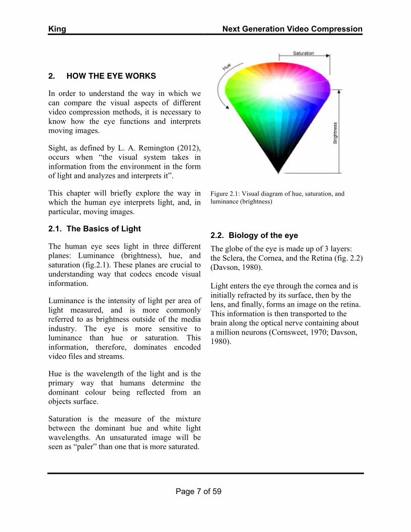
The human eye sees light in three different planes: Luminance (brightness), hue, and saturation (fig.2.1). These planes are crucial to understanding way that codecs encode visual information.
Luminance is the intensity of light per area of light measured, and is more commonly referred to as brightness outside of the media industry. The eye is more sensitive to luminance than hue or saturation. This information, therefore, dominates encoded video files and streams.
Hue is the wavelength of the light and is the primary way that humans determine the dominant colour being reflected from an objects surface.
Saturation is the measure of the mixture between the dominant hue and white light wavelengths. An unsaturated image will be seen as “paler” than one that is more saturated.
Figure 2.1: Visual diagram of hue, saturation, and luminance (brightness)
2.2. Biology of the eye The globe of the eye is made up of 3 layers: the Sclera, the Cornea, and the Retina (fig. 2.2) (Davson, 1980). Light enters the eye through the cornea and is initially refracted by its surface, then by the lens, and finally, forms an image on the retina. This information is then transported to the brain along the optical nerve containing about a million neurons (Cornsweet, 1970; Davson, 1980).
King Next Generation Video Compression
Page 8 of 59
Figure 2.2: Biology of the eye
2.2.1. Rods and Cones
The rods and cones are photoreceptive cells contained in the retina and form the system that interprets hue, saturation, and luminance.
The rod cells interpret luminance only, and the cones interpret colour information. The cones differ in the wavelengths they perceive and are categorized as being red, green, and blue (RGB) photoreceptors (Cornsweet, 1970). Humans are, therefore, a trichromatic species. This is the reason that colour video is designed to reproduce three colours that can be combined to display almost any colour perceivable in the visible spectrum.
2.2.2. Sight Impairments
As the human eye is so complex, small genetic mutations can cause issues to arise with the way that it processes information. One of the most common such issues is monochromacy, or colour blindness. This is a condition where the retina only contains the rod photoreceptors;
therefore, it is unable to distinguish between different colours.
A similar condition, dichromacy, is diagnosed when the retina only contains two of the three photoreceptors needed to perceive the full colour spectrum. A dichromat cannot correctly identify certain portions of the visible light spectrum, depending on which type of photoreceptor their retina is missing (Cornsweet, 1970).
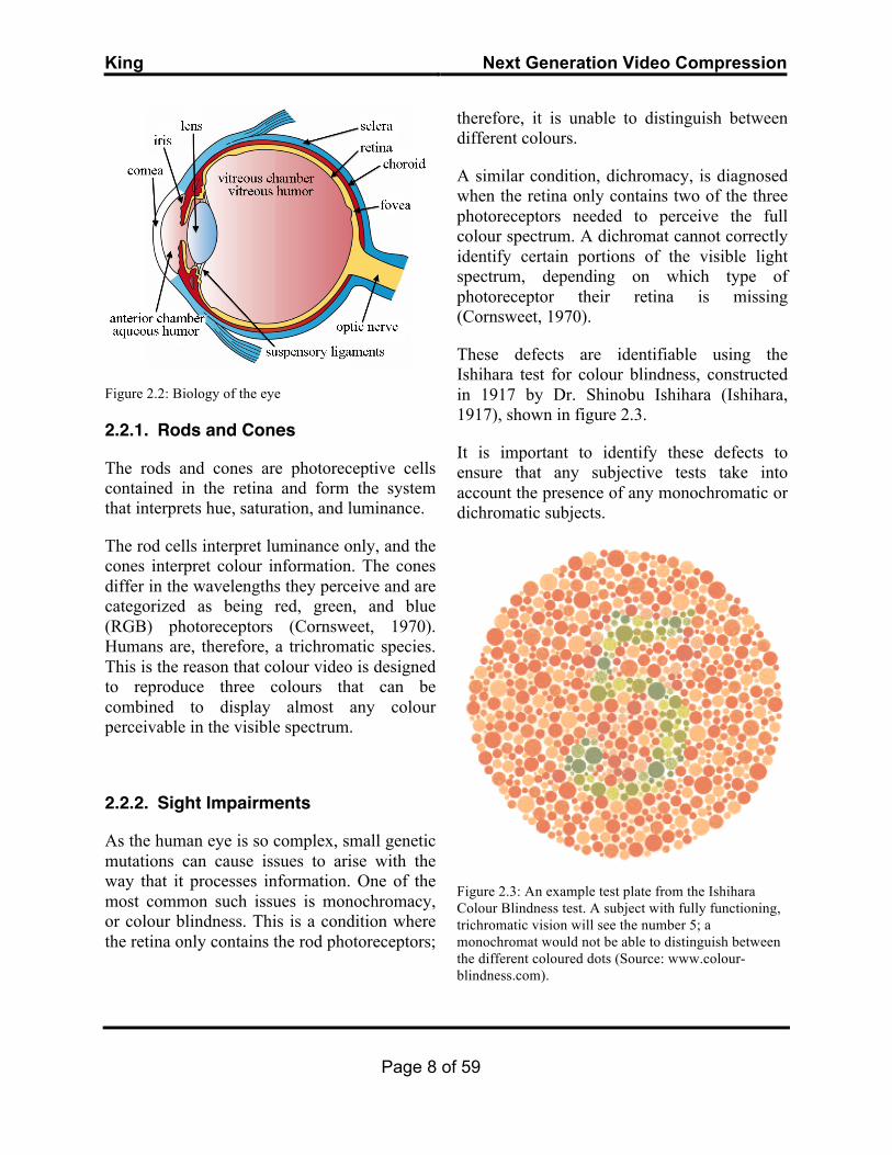
These defects are identifiable using the Ishihara test for colour blindness, constructed in 1917 by Dr. Shinobu Ishihara (Ishihara, 1917), shown in figure 2.3.
It is important to identify these defects to ensure that any subjective tests take into account the presence of any monochromatic or dichromatic subjects.
Figure 2.3: An example test plate from the Ishihara Colour Blindness test. A subject with fully functioning, trichromatic vision will see the number 5; a monochromat would not be able to distinguish between the different coloured dots (Source: www.colour-blindness.com).
King Next Generation Video Compression
Page 9 of 59
2.3. Perception of Motion Pictures
Motion pictures are created using a series of still images shown in quick succession. This creates the illusion of constant motion and is the basis of all cinematography.
Two of the main traits that are useful in creating this illusion are the persistence of vision and the critical flicker-fusion threshold (CFF).
The persistence of vision is how long an image is retained on the retina after the light source has been removed. This varies depending on the angle the source is approaching the retina from, but from an optimal viewing angle, images are retained on the retina for 40-60mS (Hardy, 1919).
In association with this is the critical flicker-fusion threshold (CFF), which is the point at which a light source alternating between bright flashes and no light, is perceived as a constant light without any flickering. It is determined by the relation between the intensity of the light source, and the frequency of intermittence, in cycles per minute. This means that higher luminance increases the CFF, meaning that for brighter light sources, more cycles per minute are required to perceive a constant source (Landis, 1954).
3. EARLY COMPRESSION STANDARDS
A need for digital video compression was realized when it became apparent that technological advancements, such as the compact disk and the internet, would create a medium for digital media to be stored and transmitted more freely. This prompted the
International Telecommunications Union (ITU, formerly CCITT) to develop a standard to allow for such methods of storage and transmission to be transparent worldwide; the first, most practical, of which was the ITU-T recommendation H.261.
A lot of the early techniques used for video compression were based on those used for image compression, such as JPEG.
3.1. ITU-T H.261
ITU-T Recommendation H.261 was designed between 1988 and 1989. The recommendation describes “the video coding and decoding methods for the moving picture component of audiovisual services at the rates of p x 64 Kbps, where p is in the range 1 to 30”. The goal of the recommendation was to develop a video encoding method that would enable efficient video conferencing across ADSL networks (International Telecommunications Union, 1988).
The codec uses inter-frame prediction to remove temporal redundancy, and the Discrete Cosine Transform (For a description and example of the DCT see Glossary) to remove spatial redundancy.
Other, optional, features of the codec include: motion compensation, and Forward Error Correction (FEC) to enable the decoder to make an informed estimation of any missing data.
One key aspect of the recommendation is that it specifies that it will only work for progressive motion pictures.
The development of the H.261 codec paved the way for future codec development, and is
King Next Generation Video Compression
Page 10 of 59
the first in the H.26x series of codecs that are explored later in this document.
3.2. Further developments
H.261 lead to the development of two other key, consumer level, codecs from the 1990s: Cinepak and Indeo.
Cinepak, developed by Supermac, was one of the first popular codecs used on PCs. After its release in 1991, it was incorporated into Apple’s Quicktime in 1992, and then into Windows in 1993 (Segaretro.org, 2014).
It used very similar compression methods to H.261, but fell out of favour to MPEG-2.
Indeo was developed in 1992 by Intel for the emerging video conferencing industry. It encoded YUV video in an asymmetrical way, which meant that encoding the video was more time consuming than decoding it. In addition to this, Indeo was a scalable codec, meaning that less powerful computers could decode the video at lower frame rates or frame sizes, than more powerful machines (Delargy, 1996). These features made the codec very attractive for the low powered computers of the 1990s, but it too fell out of favour to the rise of MPEG.
4. MPEG DEVELOPMENT
The Moving Picture Experts Group (MPEG) was formed in 1988 by the International Standards Organisation (ISO) to address the need for a common video compression standard. MPEG took the approach of standardising the way that a decoder would interpret a bit stream, as opposed to the way that an encoder would create one (Watkinson, 2008).
4.1. MPEG-1
Their first standard, MPEG-1 (ISO 11172), was released in 1992. It used similar encoding methods to those used in the JPEG, and was largely an extension of the H.261 codec (Ghanbari, 1999), with the goal of encoding video at the same rate as conventional CDs (1.5Mb/s) following the same principal of asymmetry as in Indeo.
This standard formed the basis for all subsequent MPEG standards, introducing features such as elementary stream syntax, bi-directional motion compensation (B frames), a Group of Pictures (GOP), buffering, macroblocks, and rate control; however it did not support interlaced or HD video and was therefore unsuitable for digital television broadcasting (Watkinson, 2004).
4.1.1. Group of Pictures (GOP)
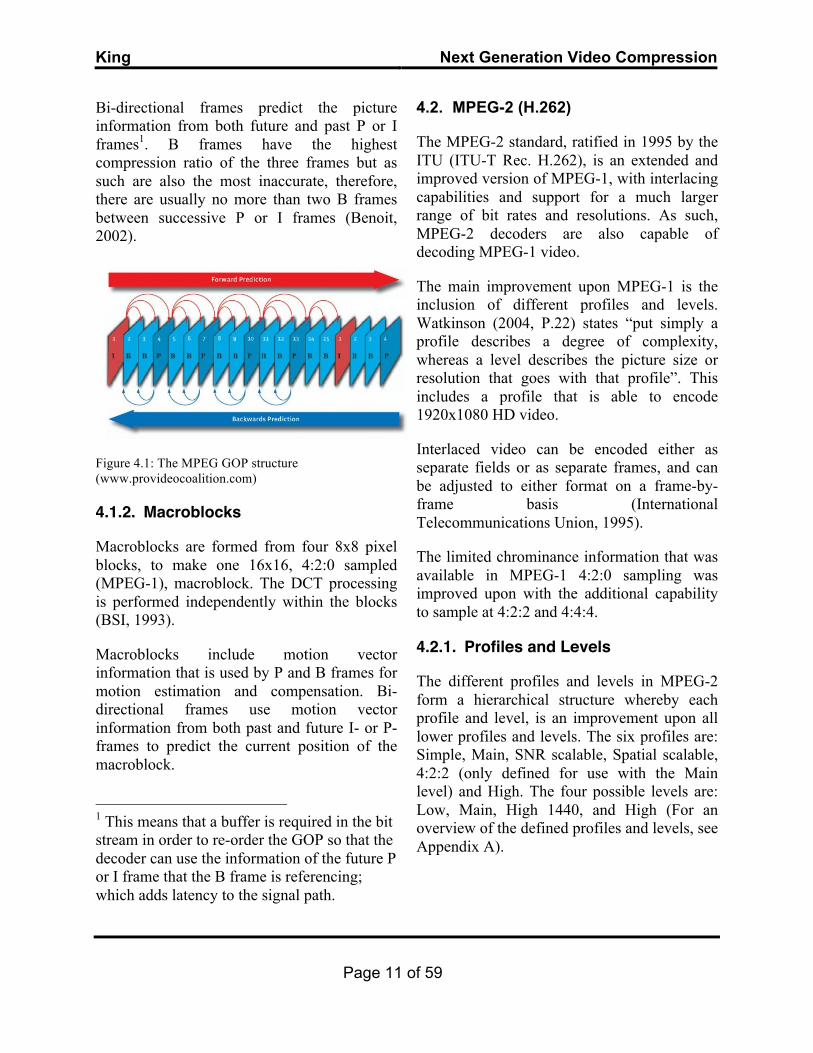
In MPEG1, and subsequent standards, there are three types of frame that are used to construct a video sequence: Intra (I) frames, Predictive (P) frames and Bi-directional (B) frames (Figure 4.1). These frames form what is known as a Group of Pictures (GOP), where the start of each GOP is indicated by an I frame.
Intra frames have the lowest compression ratio as they only use intra-coding to remove spatial redundancy. Therefore, I frames don’t reference other frames, but are used as a reference by P and B frames.
Predictive frames use information from the previous P or I frame to predict the information in the present frame. This reduces both spatial and temporal redundancy.
King Next Generation Video Compression
Page 11 of 59
Bi-directional frames predict the picture information from both future and past P or I frames1. B frames have the highest compression ratio of the three frames but as such are also the most inaccurate, therefore, there are usually no more than two B frames between successive P or I frames (Benoit, 2002).
Figure 4.1: The MPEG GOP structure (www.provideocoalition.com)
4.1.2. Macroblocks
Macroblocks are formed from four 8x8 pixel blocks, to make one 16x16, 4:2:0 sampled (MPEG-1), macroblock. The DCT processing is performed independently within the blocks (BSI, 1993).
Macroblocks include motion vector information that is used by P and B frames for motion estimation and compensation. Bi-directional frames use motion vector information from both past and future I- or P- frames to predict the current position of the macroblock.
1 This means that a buffer is required in the bit stream in order to re-order the GOP so that the decoder can use the information of the future P or I frame that the B frame is referencing; which adds latency to the signal path.
4.2. MPEG-2 (H.262)
The MPEG-2 standard, ratified in 1995 by the ITU (ITU-T Rec. H.262), is an extended and improved version of MPEG-1, with interlacing capabilities and support for a much larger range of bit rates and resolutions. As such, MPEG-2 decoders are also capable of decoding MPEG-1 video.
The main improvement upon MPEG-1 is the inclusion of different profiles and levels. Watkinson (2004, P.22) states “put simply a profile describes a degree of complexity, whereas a level describes the picture size or resolution that goes with that profile”. This includes a profile that is able to encode 1920x1080 HD video.
Interlaced video can be encoded either as separate fields or as separate frames, and can be adjusted to either format on a frame-by-frame basis (International Telecommunications Union, 1995).
The limited chrominance information that was available in MPEG-1 4:2:0 sampling was improved upon with the additional capability to sample at 4:2:2 and 4:4:4.
4.2.1. Profiles and Levels
The different profiles and levels in MPEG-2 form a hierarchical structure whereby each profile and level, is an improvement upon all lower profiles and levels. The six profiles are: Simple, Main, SNR scalable, Spatial scalable, 4:2:2 (only defined for use with the Main level) and High. The four possible levels are: Low, Main, High 1440, and High (For an overview of the defined profiles and levels, see Appendix A).
King Next Generation Video Compression
Page 12 of 59
The main profile, at main level, is used in Europe by DVB for standard definition television (Digital Video Broadcasting, 2014).
The simple profile doesn’t support B frames and is only defined at main level, it is therefore relatively easy for less powerful hardware to encode and decode. The lack of B frames also means that there will be less latency in the signal chain.
Scalable Profiles
Three of the defined profiles have the capability to transmit a scalable signal that can be decoded at two levels of quality. This is designed to provide resilience in the signal chain (the base signal is sent with a higher priority), and also reduce the bandwidth needed to transmit two signals of different quality e.g. an SD and HD signal.
The SNR (Signal to Noise Ratio) profile creates scalable signals by transmitting a base, “noisy” signal, and a noise-cancelling, enhancement signal.
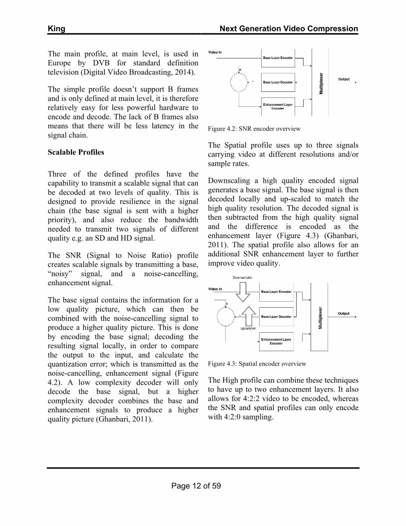
The base signal contains the information for a low quality picture, which can then be combined with the noise-cancelling signal to produce a higher quality picture. This is done by encoding the base signal; decoding the resulting signal locally, in order to compare the output to the input, and calculate the quantization error; which is transmitted as the noise-cancelling, enhancement signal (Figure 4.2). A low complexity decoder will only decode the base signal, but a higher complexity decoder combines the base and enhancement signals to produce a higher quality picture (Ghanbari, 2011).
Figure 4.2: SNR encoder overview
The Spatial profile uses up to three signals carrying video at different resolutions and/or sample rates.
Downscaling a high quality encoded signal generates a base signal. The base signal is then decoded locally and up-scaled to match the high quality resolution. The decoded signal is then subtracted from the high quality signal and the difference is encoded as the enhancement layer (Figure 4.3) (Ghanbari, 2011). The spatial profile also allows for an additional SNR enhancement layer to further improve video quality.
Figure 4.3: Spatial encoder overview
The High profile can combine these techniques to have up to two enhancement layers. It also allows for 4:2:2 video to be encoded, whereas the SNR and spatial profiles can only encode with 4:2:0 sampling.
King Next Generation Video Compression
Page 13 of 59
The maximum number of possible enhancement layers for each scalable profile can be seen in Appendix B.
4.3. MPEG-4 Part 10 (H.264/AVC)
In 2001; recognising that the cost of processing power and storage had reduced; and that network capabilities had been improved enormously since the development of H.262; the ITU Video Coding Expert Group (VCEG), and the ISO Moving Picture Expert Group (MPEG), joined together to form the Joint Visual Team (JVT) and begin development of the H.264 codec; the first edition of which was approved in 2003 (ITU, 2013).
The resulting standard, sometimes referred to as Advanced Video Coding (AVC), is an improved and extended version of the MPEG-2 standard, and, since its conception, has replaced many codecs as the default choice in a wide range of applications; from video telephony to HD video broadcasting.
The standard was developed with the same philosophy of an asymmetrical signal chain and, in the case of H.264, the resulting encoder is typically eight times more complex than an MPEG-2 encoder (Ibrahim, 2007).
H.264 introduces a lot of new features to the MPEG family of codecs (ITU, 2013), including:
• Improved error resilience
• Low delay mode for telecommunications
• Slices
• A de-blocking filter
• B frame referencing
• Multiple-frame referencing for P- and B-frames
• DCT replaced by a transform with an exact inverse transform
• Two new types of entropy coding to replace Variable Length Coding
• New and improved methods of intra and inter coding
4.3.1. Slices
One of the major differences between H.264 and earlier standards is the new way of looking at a picture in terms of slices instead of whole frames. This can be done in three different ways:
• By looking at a frame as one slice
• By dividing the frame into slices with equal numbers of macroblocks; resulting in varying packet sizes for each slice
• By dividing the frame into slices with equal packet size; resulting in varying numbers of macroblocks per slice
It also means that instead of I-, P-, and B-frames, I-, P-, and B-slices are generated; with the addition of two new slice types: SP (Switching Predictive) and SI (Switching Intra) slices.
All slices representing a picture do not need to be of the same type, but in practice this is most commonly the case; therefore in most circumstances, unless stated otherwise, it is
King Next Generation Video Compression
Page 14 of 59
still acceptable to refer to frames as I-, P-, and B-frames (Ghanbari, 2011).
SP and SI Slices
These new types of slice replace I-frames in a video stream as a point where switching to a stream of a different bit-rate or resolution is possible. As they use inter frame prediction they use less bandwidth than I frames and are therefore more efficient. They also have applications in splicing, random access, fast forwarding, rewinding, and error recovery.
In error recovery, an SP frame is sent to the decoder, referencing a frame that was correctly decoded, to create a point where the decoder can re-synchronise with the encoder (Ghanbari, 2011).
4.3.2. Intra Coding
Spatial prediction in H.264 references decoded pixel blocks above and to the left of the current block to make a reasonable estimation of the luminance value of each pixel within the current block. This is based upon the idea that adjacent macroblocks tend to have similar textures. However, since adjacent blocks may be from P- or B-slices, data from these blocks is not used for the spatial prediction process to avoid error propagation in the signal chain.
There are three main types of intra-coding for the luminance signal that are used in H.264, with varying levels of accuracy dependent upon the complexity of the picture being encoded.
Intra 4x4
Intra 4x4 is used for the most detailed areas of an image, and encodes at block level. This
method spatially predicts pixel values in 8 different directional modes, or an average (DC) mode, from the neighbouring blocks. This reduces prediction error as pixels are predicted in the same orientation as the texture, or in DC mode if the block comprises of a single luminance value. For a table of the different Intra 4x4 modes, see Appendix C.
A similar intra coding method, Intra 8x8, uses the same technique.
Intra 16x16
Intra 16x16 treats the macroblock as a whole and only has four modes, which operate in a similar way to the equivalent Intra 4x4 modes. These are horizontal, vertical, average (DC), and plane. In plane mode, pixels are predicted with reference to the pixels both adjacent, and above the macroblock being encoded.
Intra 16x16 is much more efficient for areas where there is less detail as it uses much less data than Intra 4x4.
Chrominance information is encoded using the same techniques as Intra 16x16 but it operates on 8x8 blocks of chrominance.
I_PCM
In I_PCM mode, raw PCM data is recorded without prediction of transformation in order to retain all of the macroblock information. This is used for very high quality encoding.
4.3.3. Inter Coding
Inter coding in H.264 introduces 3 main features that were not present in previous standards (Ghanbari, 2011):
King Next Generation Video Compression
Page 15 of 59
• Variable block sizes for motion estimation
• Quarter-pixel precision for motion vectors
• Multiple referencing for P- and B-frames
These new features mean that inter frame prediction is more complex and more accurate than inter frame prediction used in MPEG-2.
Variable Block Sizes
The 16x16 macroblocks that were used for motion estimation in MPEG-2 are inaccurate if the moving object that is being encoded is smaller than the size of the macroblock or crosses, but does not completely fill, multiple macroblocks. This is most noticeable at lower resolutions (Watkinson, 2004).
In H.264, blocks can be encoded at multiple sizes, ranging from 4x4 pixels to 16x16. This also includes rectangular blocks in sizes such as 16x8 and 4x8.
In doing this the motion estimation is more accurate than MPEG-2, however, smaller block sizes means a larger volume of data overhead.
Quarter-Pixel Precision for Motion Vectors
MPEG-2 could encode motion vectors with half-pixel precision, whereas H.264 can encode luminance sample motion vectors with quarter-pixel precision, and chrominance sample motion vectors with up to one-eighths pixel precision. This obviously results in much more accurate motion estimation.
Multiple-Frame Referencing for P- and B-
Frames
In MPEG-1 and MPEG-2, P-frames were only able to reference one frame, and B-frames could reference a maximum of two frames. H.264 allows multiple-frame referencing (known as weighted prediction) of up to 16 frames for both P- and B-frames meaning that inter frame prediction results in much better quality. This also means that different macroblocks within the same picture can be predicted using blocks from multiple different frames. This reduces the amount of data that needs to encoded, and improves accuracy, as only the smallest difference between macroblocks is encoded (Ghanbari, 2011).
In addition to this, H.264 allows B-frames to be used as references, although this feature is rarely exploited due to the inevitable inaccuracies that it would present in comparison to I- and P-frame referencing.
4.3.4. Transformation
In the same way that previous standards remove the redundancy from the encoded pixel values in intra and inter coding using the Discrete Cosine Transform, H.264 uses a more accurate variation of the DCT known as the Integer Transform. This uses a 4x4 variation on the 8x8 DCT which has an exact inverse transform, eliminating all transformation mismatches that were present in the DCT method, therefore allowing lossless compression.
4.3.5. Entropy Coding
Prior to the release of H.264 most codecs used Variable Length Coding to encode the entropy in a lossless format. H.264 introduces two new
King Next Generation Video Compression
Page 16 of 59
types of entropy coding: Context-Adaptive Variable Length Coding (CAVLC), and Context-Adaptive Binary Arithmetic Coding (CABAC).
Before either CAVLC or CABAC are applied to the data, it is zig-zag scanned across the block, from the most frequent value to the least frequent to produce one string containing all values.
CAVLC
In CAVLC, typical properties of the transform coefficients (results of the transform), found after quantization and transformation, are exploited to code the entropy more efficiently (Heo, Kim, and Ho, 2010).
These properties are:
• Transform coefficients typically contain high numbers of zeroes; particularly in high frequency areas
• Most nonzero coefficients are sequences of ±1s (Trailing 1s) with equal probability
• The volume of nonzero coefficients tends to be higher towards the low frequency regions of the transform
• Nonzero values in adjacent blocks tend to be highly correlated so they can use the same look-up tables
Taking advantage of these properties, CAVLC then applies the following steps:
1. The nonzero coefficients and trailing 1s are encoded with a combined codeword
2. The sign of each trailing 1 is encoded using a one bit codeword
3. The absolute value (ignoring the sign) of each nonzero coefficient is encoded using the look up tables, and their signs are encoded using a one bit codeword
4. The number of all zeroes before the last nonzero coefficient is encoded
5. The number of zeroes preceding each nonzero coefficient is encoded
CABAC
CABAC is based on arithmetic coding which has been proven to produce much better levels of compression than Variable Length Coding; however, it is also much more computationally expensive (Seabrook, 1989).
CAVLC requires at least one bit to represent each symbol, which is inefficient for symbols with a probability less than 0.5 (Ghanbari, 2011). In arithmetic coding, blocks of symbols are assigned a single code word, meaning that it can achieve an average of less than one bit per symbol. This is done by subdividing values into blocks between 0 and 1, according to the probability of each symbol in the word, until a value is found that can represent the whole word. The resulting value is then binarised (converted so that it can be represented using binary) (Mathematicalmonk, 2011).
King Next Generation Video Compression
Page 17 of 59
In addition to this, arithmetic coding separates the statistical modelling from the coding so any statistical model can be used along side it. This means that context adaptation is very flexible but to limit the number of models that are used in one bit stream, and therefore limiting the amount of extra data needed to be transmitted to decode the stream, H.264 only uses four different types of statistical analysis.
4.3.6. Profiles Overview
Similar to previous MPEG standards, H.264 has different profiles designed to be used for different applications, with varying complexity and compression ratios.
Baseline Profile
The baseline profile is the least complex profile, and therefore has the lowest compression ratio. It was designed for real time applications, such as video telephony and video conferencing.
This profile only uses I- and P-frames, uses the simpler CAVLC entropy coding, and large amounts of built in error resiliency to cope with hostile networks.
Main Profile
This profile uses I-, P-, and B-frames, and can select between using CAVLC and CABAC entropy coding. It also introduces the capability to encode interlaced video.
The main profile has the highest possible compression ratio but does not include any error-resilience tools as its use is designed for video storage (High-Definition DVDs) and transmission on ‘clean’ networks.
Another key feature of the main profile is the use of weighted prediction.
Extended Profile
This profile includes all of the features of the baseline profile, with the added features of weighted prediction and B-frames. However, this profile does not support interlacing or CABAC entropy coding.
The unique feature of this profile is the addition of SP- and SI-frames for switching between video streams. Therefore, the best application for this profile is online video streaming.
High Profiles
The high profiles are an extension of the main profile with the additional capability of adaptive block sizes for intra coding.
There are 4 high profiles that use the features above but different bit and sampling rates:
• High – 8 bit, 4:2:0
• High 10 – 10 bit, 4:2:0
• High 4:2:2 – 10 bit, 4:2:2
• High 4:4:4 – 12 bit, 4:4:4
An overview of the key features of each profile can be seen in figure 4.4.

King Next Generation Video Compression
Page 18 of 59
Figure 4.4: An overview of the H.264 profiles key features (Richardson, 2003)
5. HEVC (HIGH EFFICIENCY VIDEO CODING)
Work on HEVC (ITU Rec. H.265) began in 2010 by the Joint Visual Team (JVT) who had previously developed the Advanced Video Coding (MPEG 4 part 10, ITU Rec. H.264) standard.
HEVC was developed to address the need for better video coding efficiency of HD and post-HD (4K, 8K) video. The main focus of the standard is on increased video resolution and the use of parallel processing architectures.
The first version of the standard was released in January 2013, followed by the release of the second version in October 2014.
The standard introduces several new features that have not been present in previous MPEG or ITU coding standards, including:
• A new Quadtree based coding structure that replaces the macroblock structure
• Advanced Motion Vector Prediction
• Quarter-sample Motion Compensation accuracy
• 35 intra picture prediction modes (compared with 9 in H.264)
• Improved CABAC entropy coding
• Enhanced parallelisation features and the introduction of Tiles and Wavefront Parallel Processing
• 2-Byte Network Abstraction Layer (NAL) packet headers that identify the packet more efficiently
• Compatibility with ITU rec. 2020 for Higher Dynamic Range colour
5.1. Quadtree Coding Structure
The Quadtree coding structure used in HEVC introduces improved flexibility and variety in the way that the codec segments a picture into blocks of pixels. The quadtree coding structure allows the codec to split each unit down into quarters until the necessary pixel block size is reached. This is done to efficiently encode each section of the picture according to the amount of detail contained within it. Appendix D demonstrates how HEVC partitions a picture using fewer blocks compared with H.264.
Each unit in the Quadtree structure is comprised of equivalent luminance and chrominance blocks.
King Next Generation Video Compression
Page 19 of 59
In previous standards a macroblock with a fixed size of 16x16 luminance samples was used. The equivalent unit in HEVC, known as the Coding Tree Unit (CTU), can be comprised of 16x16, 32x32, or 64x64 pixels meaning that greater compression ratios can be achieved (Sullivan et al, 2012). The CTU size is defined at the start of a video sequence and remains the same throughout.
The CTUs can then be further broken down into Coding Units (CUs). The CU can range from 8x8 pixels in size, to the same size as the CTU it is contained within, and each CU can be broken down into smaller CUs independently. The CU defines an area using the same prediction mode (intra or inter).
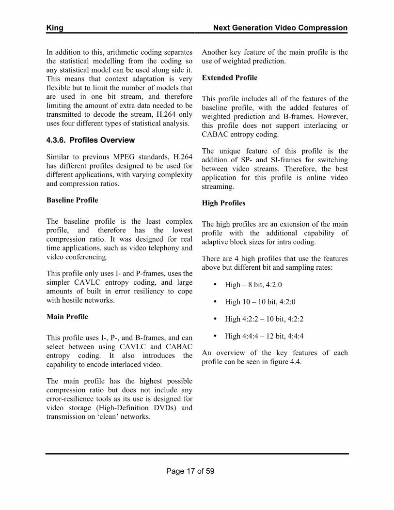
The CU is then further split into Prediction Units (PUs), which are used to store motion vector or intra-picture prediction information (depending on the prediction mode of the CU). A PB can be MxN in size (rectangular) or MxM (square), and is equal to, or smaller than, the size of the CU (Figure 5.1).
Figure 5.1: Prediction Block Sizes
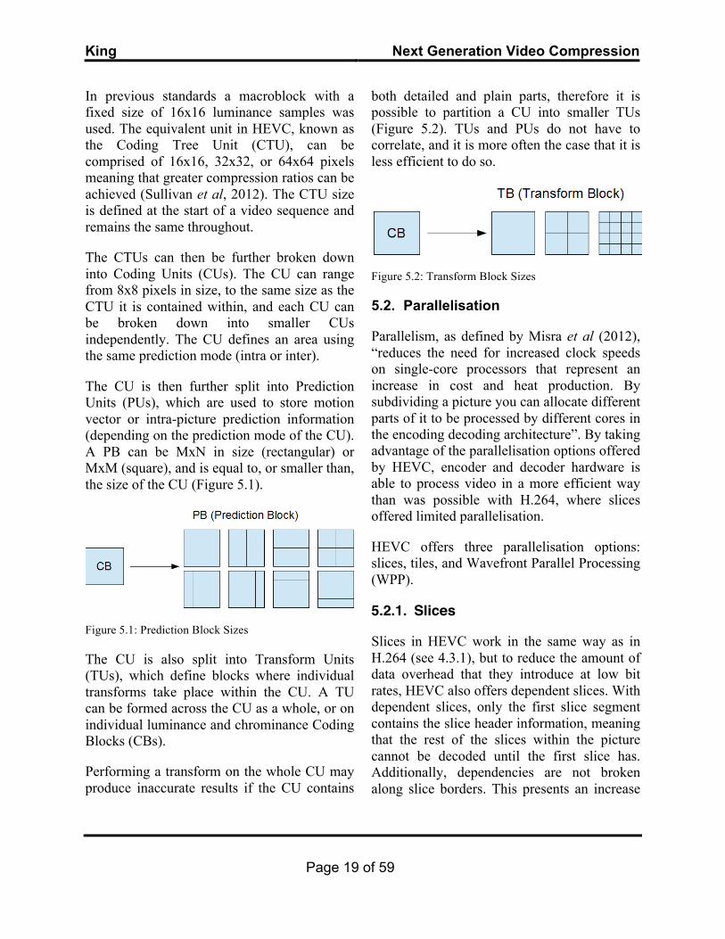
The CU is also split into Transform Units (TUs), which define blocks where individual transforms take place within the CU. A TU can be formed across the CU as a whole, or on individual luminance and chrominance Coding Blocks (CBs).
Performing a transform on the whole CU may produce inaccurate results if the CU contains
both detailed and plain parts, therefore it is possible to partition a CU into smaller TUs (Figure 5.2). TUs and PUs do not have to correlate, and it is more often the case that it is less efficient to do so.
Figure 5.2: Transform Block Sizes
5.2. Parallelisation
Parallelism, as defined by Misra et al (2012), “reduces the need for increased clock speeds on single-core processors that represent an increase in cost and heat production. By subdividing a picture you can allocate different parts of it to be processed by different cores in the encoding decoding architecture”. By taking advantage of the parallelisation options offered by HEVC, encoder and decoder hardware is able to process video in a more efficient way than was possible with H.264, where slices offered limited parallelisation.
HEVC offers three parallelisation options: slices, tiles, and Wavefront Parallel Processing (WPP).
5.2.1. Slices
Slices in HEVC work in the same way as in H.264 (see 4.3.1), but to reduce the amount of data overhead that they introduce at low bit rates, HEVC also offers dependent slices. With dependent slices, only the first slice segment contains the slice header information, meaning that the rest of the slices within the picture cannot be decoded until the first slice has. Additionally, dependencies are not broken along slice borders. This presents an increase
King Next Generation Video Compression
Page 20 of 59
in efficiency, but also increases the possibility of considerable errors to occur due to packet loss or corruption in the first slice. Dependent slices can be further combined with tiles and WPP for even greater efficiency that will allow for a large reduction in latency for real-time applications.
As with H.264 “Slice partitioning can be defined by the MTU [Maximum Transmission Unit] of the network or pixel processing constraints such as the amount of CTBs that should be contained in each slice.” (Misra et al, 2013, P.970).
5.2.2. Tiles
Tiles are independently coded, rectangular regions of a picture formed along the intersection of CTU rows and columns. They are processed in raster scan order (left to right, moving down the picture), as are the CTUs contained within them.
Tiles share header information to improve the coding efficiency, and the location of tiles within a picture is described in a packet header that contains the locations of the CTU row and column intersections.
As entropy coding and reconstruction is independent on each tile, parallelisation is achieved by processing tiles on separate cores simultaneously. This also reduces the amount of buffering required on each core, as the buffer only needs to store motion vector and intra-picture coding information for the tiles it is processing, and not the whole bitstream.
One key advantage of tiles is Region of Interest (ROI) signalling. Tiles can that are signalled as ROI contain the most important region of a picture that needs to be reproduced the most accurately. When a tile is identified
as ROI, the most capable core is selected to process it, ensuring the best possible reproduction.
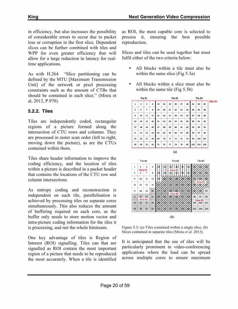
Slices and tiles can be used together but must fulfil either of the two criteria below:
• All blocks within a tile must also be within the same slice (Fig 5.3a)
• All blocks within a slice must also be within the same tile (Fig 5.3b)
Figure 5.3: (a) Tiles contained within a single slice. (b) Slices contained in separate tiles (Misra et al, 2013).
It is anticipated that the use of tiles will be particularly prominent in video-conferencing applications where the load can be spread across multiple cores to ensure maximum
King Next Generation Video Compression
Page 21 of 59
efficiency and minimum latency; particularly in mobile devices where multiple cores are becoming more commonplace (Misra et al, 2013).
5.2.3. Wavefront Parallel Processing (WPP)
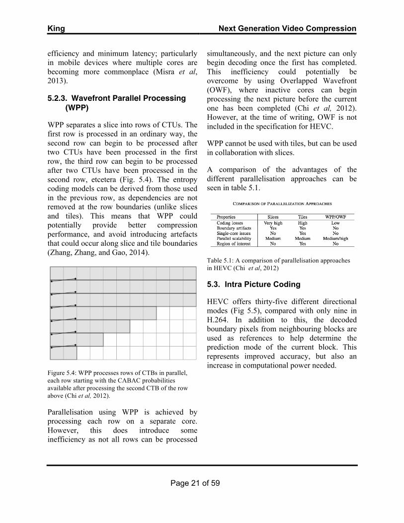
WPP separates a slice into rows of CTUs. The first row is processed in an ordinary way, the second row can begin to be processed after two CTUs have been processed in the first row, the third row can begin to be processed after two CTUs have been processed in the second row, etcetera (Fig. 5.4). The entropy coding models can be derived from those used in the previous row, as dependencies are not removed at the row boundaries (unlike slices and tiles). This means that WPP could potentially provide better compression performance, and avoid introducing artefacts that could occur along slice and tile boundaries (Zhang, Zhang, and Gao, 2014).
Figure 5.4: WPP processes rows of CTBs in parallel, each row starting with the CABAC probabilities available after processing the second CTB of the row above (Chi et al, 2012).
Parallelisation using WPP is achieved by processing each row on a separate core. However, this does introduce some inefficiency as not all rows can be processed
simultaneously, and the next picture can only begin decoding once the first has completed. This inefficiency could potentially be overcome by using Overlapped Wavefront (OWF), where inactive cores can begin processing the next picture before the current one has been completed (Chi et al, 2012). However, at the time of writing, OWF is not included in the specification for HEVC.
WPP cannot be used with tiles, but can be used in collaboration with slices.
A comparison of the advantages of the different parallelisation approaches can be seen in table 5.1.
Table 5.1: A comparison of parallelisation approaches in HEVC (Chi et al, 2012)
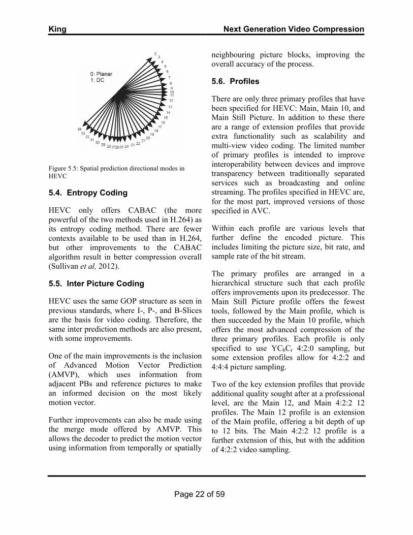
5.3. Intra Picture Coding
HEVC offers thirty-five different directional modes (Fig 5.5), compared with only nine in H.264. In addition to this, the decoded boundary pixels from neighbouring blocks are used as references to help determine the prediction mode of the current block. This represents improved accuracy, but also an increase in computational power needed.
King Next Generation Video Compression
Page 22 of 59
Figure 5.5: Spatial prediction directional modes in HEVC
5.4. Entropy Coding
HEVC only offers CABAC (the more powerful of the two methods used in H.264) as its entropy coding method. There are fewer contexts available to be used than in H.264, but other improvements to the CABAC algorithm result in better compression overall (Sullivan et al, 2012).
5.5. Inter Picture Coding
HEVC uses the same GOP structure as seen in previous standards, where I-, P-, and B-Slices are the basis for video coding. Therefore, the same inter prediction methods are also present, with some improvements.
One of the main improvements is the inclusion of Advanced Motion Vector Prediction (AMVP), which uses information from adjacent PBs and reference pictures to make an informed decision on the most likely motion vector.
Further improvements can also be made using the merge mode offered by AMVP. This allows the decoder to predict the motion vector using information from temporally or spatially
neighbouring picture blocks, improving the overall accuracy of the process.
5.6. Profiles
There are only three primary profiles that have been specified for HEVC: Main, Main 10, and Main Still Picture. In addition to these there are a range of extension profiles that provide extra functionality such as scalability and multi-view video coding. The limited number of primary profiles is intended to improve interoperability between devices and improve transparency between traditionally separated services such as broadcasting and online streaming. The profiles specified in HEVC are, for the most part, improved versions of those specified in AVC.
Within each profile are various levels that further define the encoded picture. This includes limiting the picture size, bit rate, and sample rate of the bit stream.
The primary profiles are arranged in a hierarchical structure such that each profile offers improvements upon its predecessor. The Main Still Picture profile offers the fewest tools, followed by the Main profile, which is then succeeded by the Main 10 profile, which offers the most advanced compression of the three primary profiles. Each profile is only specified to use YCbCr 4:2:0 sampling, but some extension profiles allow for 4:2:2 and 4:4:4 picture sampling.
Two of the key extension profiles that provide additional quality sought after at a professional level, are the Main 12, and Main 4:2:2 12 profiles. The Main 12 profile is an extension of the Main profile, offering a bit depth of up to 12 bits. The Main 4:2:2 12 profile is a further extension of this, but with the addition of 4:2:2 video sampling.
King Next Generation Video Compression
Page 23 of 59
5.7. Other Features
One of the most notable features of HEVC is the lack of support for interlaced video. It was decided that the decreasing distribution of interlaced video and increasingly obsolete production of interlaced monitors justified the use of progressive-only scanning; a decision which will undoubtedly influence the way that video is distributed in the future.
The way that the codec handles motion compensation has also been improved, with HEVC offering quarter-sample precision (as introduced in AVC), combined with weighted prediction and allowance for multiple reference pictures. This ultimately gives HEVC superior motion compensation accuracy compared with previous standards.
6. VP9
Development of VP9 by Google began in 2011 as part of the continuation of the Webm project, which aimed to introduce an open-source video standard to the Internet (The Webm Project, n.d.). Up until Webm was released in 2010, using VP9’s predecessor VP8, there was no freely implementable video format designed for HTML. The goal of VP9 was to produce the same quality output for 50% of the bitrate used in VP8 and H.264.
Support for VP9 is currently natively available in various web browsers including Google Chrome, Mozilla Firefox, and Opera. This widespread support has allowed Google to introduce VP9 encoding to Youtube, which they claim has enabled 25% more of their videos to be viewed in HD, and meant that they load, on average, 15% faster (Ramamoorthy, 2014).
Unfortunately, Google have not yet released a full specification for the codec, but the information in this chapter is accurate at the time of writing.
6.1. Improvements Upon VP8
The Webm Project introduces several key features in VP9 that make significant advances on VP8 and make it a viable option for many more applications than just those requiring an open-source video format for the Internet.
This includes:
• A Variable Bit-rate option
• A Constant Quality (regardless of bit-rate) option
• A Constrained Quality option that behaves like a capped VBR option
• 4:2:2 and 4:4:4 colour profiles (currently experimental)
• 10 and 12 bit video support
• Only progressive encoding (no option for interlaced video)
• Compatibility with ITU rec. 601, 709, and 2020 colour spaces, the latter of which is required for 4K video
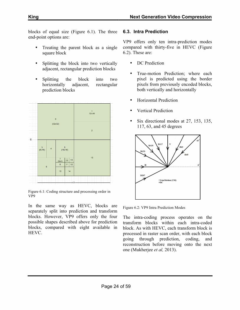
6.2. Coding Structure
VP9 uses a similar quad-tree style coding structure to that used in HEVC, with block sizes ranging from a Super-block (SB) of 64x64 to the smallest block of 4x4, processed in raster scan order. One of the key differences however is that at each block level there are three potential end-point options, and one option for further breakdown into four smaller
King Next Generation Video Compression
Page 24 of 59
blocks of equal size (Figure 6.1). The three end-point options are:
• Treating the parent block as a single square block
• Splitting the block into two vertically adjacent, rectangular prediction blocks
• Splitting the block into two horizontally adjacent, rectangular prediction blocks
Figure 6.1: Coding structure and processing order in VP9
In the same way as HEVC, blocks are separately split into prediction and transform blocks. However, VP9 offers only the four possible shapes described above for prediction blocks, compared with eight available in HEVC.
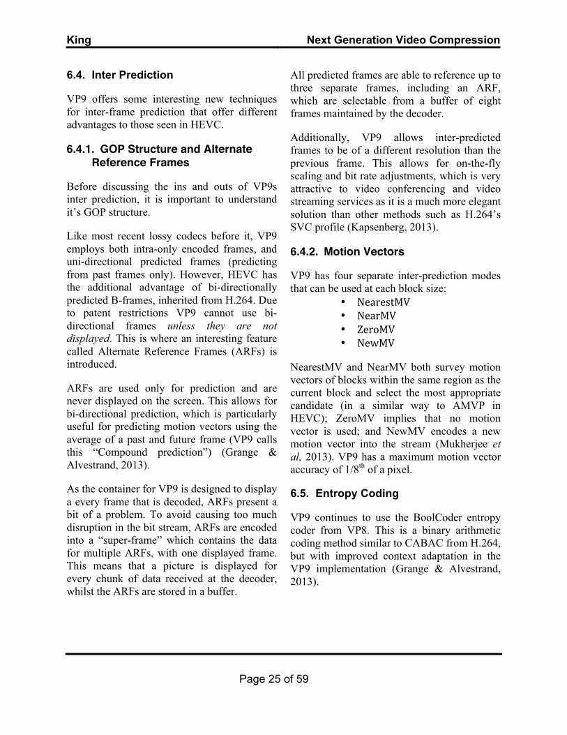
6.3. Intra Prediction
VP9 offers only ten intra-prediction modes compared with thirty-five in HEVC (Figure 6.2). These are:
• DC Prediction
• True-motion Prediction; where each pixel is predicted using the border pixels from previously encoded blocks, both vertically and horizontally
• Horizontal Prediction
• Vertical Prediction
• Six directional modes at 27, 153, 135, 117, 63, and 45 degrees
Figure 6.2: VP9 Intra Prediction Modes
The intra-coding process operates on the transform blocks within each intra-coded block. As with HEVC, each transform block is processed in raster scan order, with each block going through prediction, coding, and reconstruction before moving onto the next one (Mukherjee et al, 2013).
King Next Generation Video Compression
Page 25 of 59
6.4. Inter Prediction
VP9 offers some interesting new techniques for inter-frame prediction that offer different advantages to those seen in HEVC.
6.4.1. GOP Structure and Alternate Reference Frames
Before discussing the ins and outs of VP9s inter prediction, it is important to understand it’s GOP structure.
Like most recent lossy codecs before it, VP9 employs both intra-only encoded frames, and uni-directional predicted frames (predicting from past frames only). However, HEVC has the additional advantage of bi-directionally predicted B-frames, inherited from H.264. Due to patent restrictions VP9 cannot use bi-directional frames unless they are not displayed. This is where an interesting feature called Alternate Reference Frames (ARFs) is introduced.
ARFs are used only for prediction and are never displayed on the screen. This allows for bi-directional prediction, which is particularly useful for predicting motion vectors using the average of a past and future frame (VP9 calls this “Compound prediction”) (Grange & Alvestrand, 2013).
As the container for VP9 is designed to display a every frame that is decoded, ARFs present a bit of a problem. To avoid causing too much disruption in the bit stream, ARFs are encoded into a “super-frame” which contains the data for multiple ARFs, with one displayed frame. This means that a picture is displayed for every chunk of data received at the decoder, whilst the ARFs are stored in a buffer.
All predicted frames are able to reference up to three separate frames, including an ARF, which are selectable from a buffer of eight frames maintained by the decoder.
Additionally, VP9 allows inter-predicted frames to be of a different resolution than the previous frame. This allows for on-the-fly scaling and bit rate adjustments, which is very attractive to video conferencing and video streaming services as it is a much more elegant solution than other methods such as H.264’s SVC profile (Kapsenberg, 2013).
6.4.2. Motion Vectors
VP9 has four separate inter-prediction modes that can be used at each block size:
• NearestMV • NearMV • ZeroMV • NewMV
NearestMV and NearMV both survey motion vectors of blocks within the same region as the current block and select the most appropriate candidate (in a similar way to AMVP in HEVC); ZeroMV implies that no motion vector is used; and NewMV encodes a new motion vector into the stream (Mukherjee et al, 2013). VP9 has a maximum motion vector accuracy of 1/8th of a pixel.
6.5. Entropy Coding
VP9 continues to use the BoolCoder entropy coder from VP8. This is a binary arithmetic coding method similar to CABAC from H.264, but with improved context adaptation in the VP9 implementation (Grange & Alvestrand, 2013).
King Next Generation Video Compression
Page 26 of 59
6.6. Transformation
VP9 supports three type of transformation: The DCT as used in H.264; the Asymmetric Discrete Sine Transform (ADST), which is suggested to be more efficient than the DCT for some intra prediction (Grange & Alvestrand, 2013); and The Walsh-Hadamard Transform (WHT).
The DCT is used on all inter-coded blocks, and can be used on all blocks up to 32x32. For intra-coded blocks, a hybrid of the ADST and a 1-dimensional DCT can be used. The WHT is only used at the 4x4 level to losslessly encode intra pictures.
6.7. Parallelisation
As with HEVC, VP9 has also been designed to take advantage of increasingly common multi-core processor architectures. There are two methods of parallelisation available: frame-level parallelism and tiling.
6.7.1. Tiling
VP9 uses a similar tiling scheme to that used in HEVC, with a few subtle differences. In VP9, tiles are independently coded sub-units of a frame, but the dependencies for each tile are broken along column borders only and the tiles are spaced as evenly as possible; with the number of tiles in a frame always equalling 2n (Kapsenberg, 2013). This means that a frame containing eight tiles (4x4) can only be decoded using four threads.
6.7.2. Frame-Level Parallelism
When enabled, this mode allows the decoder to decode the entropy for successive frames in a semi-parallel manner, providing that required information from past reference frames has
already been decoded. Frames are then reconstructed sequentially as they are required to be displayed (Grange & Alvestrand, 2013).
6.8. Segmentation
Segmentation is an interesting feature that allows select areas of a frame to have certain attributes processed differently to the rest of the frame. Segments are not restricted to a certain shape, allowing flexibility in their usage (Kapsenberg, 2013; Grange & Alvestrand, 2013).
The frame is divided into eight segments, each of which can have any of four features below enabled:
Skip
This feature marks the segment as having no temporal changes in successive frames, i.e. a static background.
Alternate Quantizer
This feature is useful for marking an area that needs more (or less) detail than other segments, and changes the number of quantization levels to reflect that.
Ref
This feature enables a segment to use a different reference frame to those indicated in the frame header.
AltLf
This feature allows the segment to use a different strength of smoothing filter to the rest of the frame, which is useful for smoothing out particularly blocky areas of the picture.

King Next Generation Video Compression
Page 27 of 59
6.9. Profiles
Unfortunately, as there is no official spec for VP9, there is also no listing of the full features enabled in each profile.
However, information from the Webm Project developers (Wilkins, 2013; Ramamoorthy, 2014) suggests that there are four profiles with the following capabilities:
• Profile 0
o 4:2:0 sampling • Profile 1
o 4:2:2 and 4:4:4 sampling • Profile 2
o Same as 0 but with 10 or 12 bit encoding
• Profile 3 o Same as 1 but with 10 or 12
bit encoding
Unfortunately, there is no indication about which features will be available in each profile at the time of writing.
7. SUBJECTIVE TESTING METHODOLOGY AND EVALUATION
Having looked at the techniques that both codecs use, and developed an understanding of how they compare in theory, the next obvious step is to look at their video outputs.
In this section a description of the testing methodology and justification for the choice of encoding parameters is presented.
The chosen test methodology for conducting the subjective testing is the Double Stimulus Constant Quality Scale (DSCQS) method,
described by ITU-R BT.500 (2012). The subjective tests compare video encoded at the same bit rates by VP9 and HEVC in the UHD1 (3840x2160) resolution.
This method suggests the use of a variety of test materials, using a set presentation structure, with allowances for a mixture of both expert and non-expert participants.
7.1. Equipment
The equipment required for this method of testing is as follows:
• Encoding hardware
• A television monitor
• A decoder/playback device
• A room with the capability to be set in ideal test conditions
7.1.1. Encoding Hardware
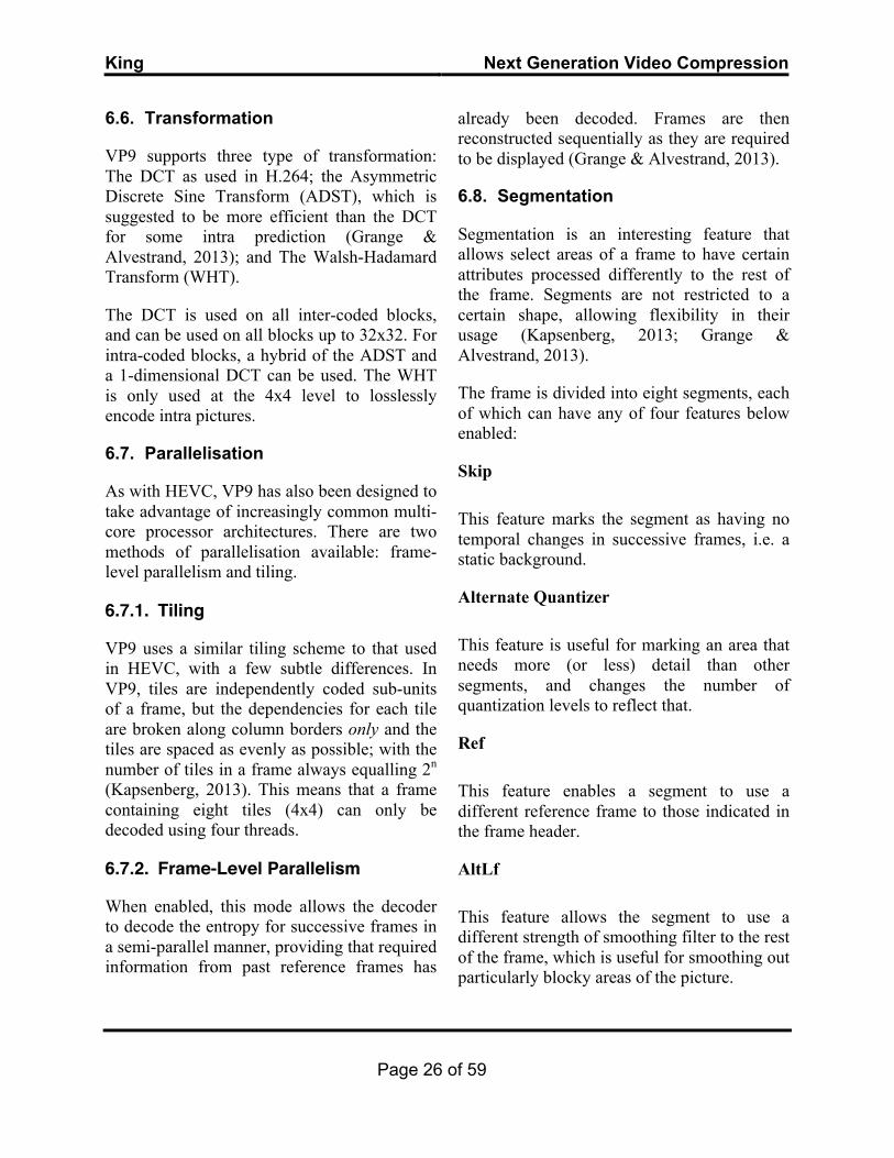
The encoding hardware used to encode the test materials was a Macbook Pro. Ideally, a dedicated server with higher computational power would be used but the practicality of transferring large files and the financial cost implications of a server with sufficient storage made this impractical. The added benefit of using a laptop to encode is that it gives additional insight into the real-world usage of the codecs using consumer level hardware. The specifications for the laptop are shown in table 7.1.
King Next Generation Video Compression
Page 28 of 59
Processor Type Intel Core i5
Processor Speed
2.4 Ghz (With turbo boost up to 2.93 Ghz, and hyper-threading)
RAM 8Gb (2x 1066Mhz DDR3 4Gb)
Available Storage
70Gb HDD
Table 7.1: Encoding hardware specification
7.1.2. Television Monitor
As the test material to be used was in the UHD1 resolution, a 4K capable television monitor was required.
The available 4K monitor was the 58-inch LED Panasonic TX-58AX802. This monitor has USB3 ports and a 4K-capable HDMI input which provided two potential methods for displaying the test material. The full television specification is available from Panasonic (n.d).
Originally, it was planned to play the test materials directly from a USB3 hard-disk drive but this would have meant re-encoding the test material to another codec that the decoder in the television was able to interpret. Subsequently, this meant re-encoding to a lossless format, in order to avoid any concatenation errors from multiple encodes, thus significantly increasing the bit rate, consequently meaning that the television would not be able to decode the material fast enough to allow smooth playback.
Therefore, it was decided that the most appropriate method would be to use external hardware connected using the 4K HDMI port on the television.
Before any testing began the levels on the monitor were checked using EBU colour bars and test signals.
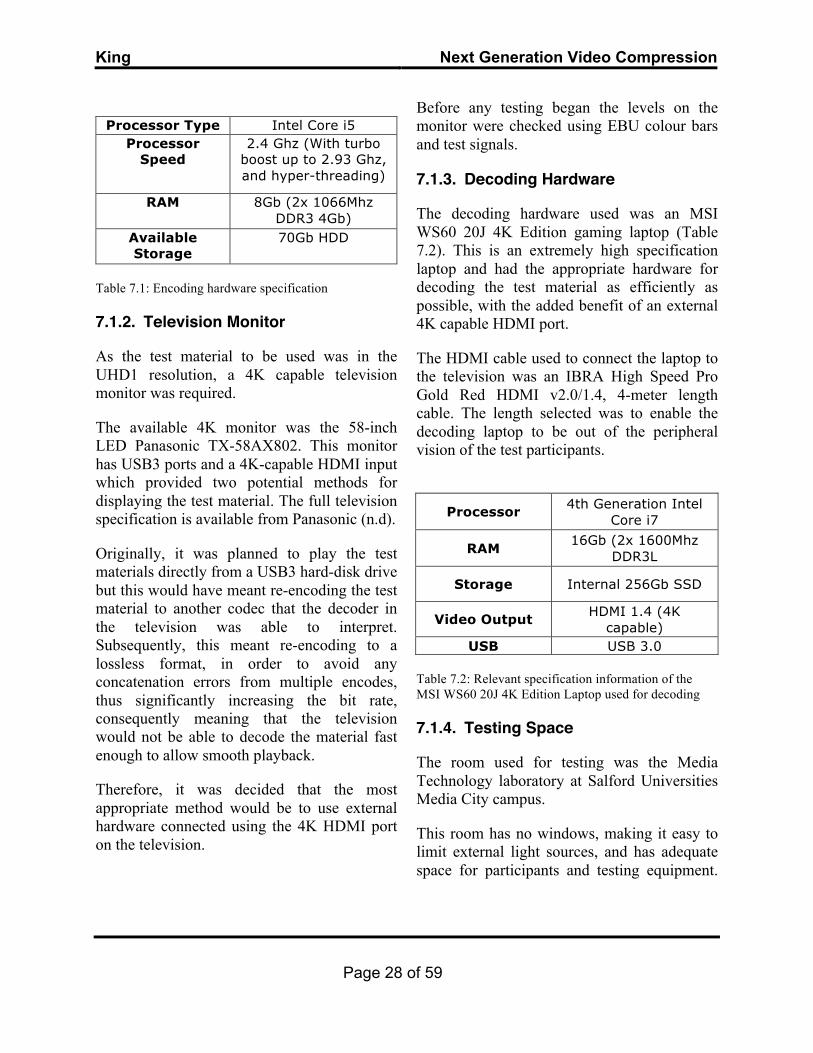
7.1.3. Decoding Hardware
The decoding hardware used was an MSI WS60 20J 4K Edition gaming laptop (Table 7.2). This is an extremely high specification laptop and had the appropriate hardware for decoding the test material as efficiently as possible, with the added benefit of an external 4K capable HDMI port.
The HDMI cable used to connect the laptop to the television was an IBRA High Speed Pro Gold Red HDMI v2.0/1.4, 4-meter length cable. The length selected was to enable the decoding laptop to be out of the peripheral vision of the test participants.
Processor 4th Generation Intel Core i7
RAM 16Gb (2x 1600Mhz DDR3L
Storage Internal 256Gb SSD
Video Output HDMI 1.4 (4K capable)
USB USB 3.0
Table 7.2: Relevant specification information of the MSI WS60 20J 4K Edition Laptop used for decoding
7.1.4. Testing Space
The room used for testing was the Media Technology laboratory at Salford Universities Media City campus.
This room has no windows, making it easy to limit external light sources, and has adequate space for participants and testing equipment.
King Next Generation Video Compression
Page 29 of 59
This made the room ideal for setting the required testing conditions.
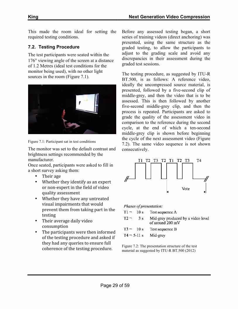
7.2. Testing Procedure The test participants were seated within the 176° viewing angle of the screen at a distance of 1.2 Metres (ideal test conditions for the monitor being used), with no other light sources in the room (Figure 7.1).
Figure 7.1: Participant sat in test conditions
The monitor was set to the default contrast and brightness settings recommended by the manufacturer. Once seated, participants were asked to fill in a short survey asking them:
• Their age • Whether they identify as an expert
or non-‐expert in the field of video quality assessment
• Whether they have any untreated visual impairments that would prevent them from taking part in the testing
• Their average daily video consumption
• The participants were then informed of the testing procedure and asked if they had any queries to ensure full coherence of the testing procedure.
Before any assessed testing began, a short series of training videos (direct anchoring) was presented, using the same structure as the graded testing, to allow the participants to adjust to the grading scale and avoid any discrepancies in their assessment during the graded test sessions.
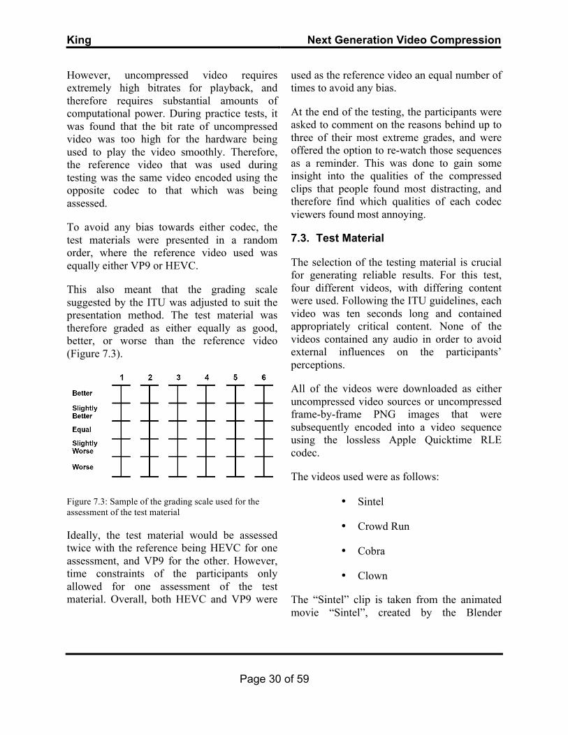
The testing procedure, as suggested by ITU-R BT.500, is as follows: A reference video, ideally the uncompressed source material, is presented, followed by a five-second clip of middle-grey, and then the video that is to be assessed. This is then followed by another five-second middle-grey clip, and then the process is repeated. Participants are asked to grade the quality of the assessment video in comparison to the reference during the second cycle, at the end of which a ten-second middle-grey clip is shown before beginning the cycle of the next assessment video (Figure 7.2). The same video sequence is not shown consecutively.
Figure 7.2: The presentation structure of the test material as suggested by ITU-R BT.500 (2012)
King Next Generation Video Compression
Page 30 of 59
However, uncompressed video requires extremely high bitrates for playback, and therefore requires substantial amounts of computational power. During practice tests, it was found that the bit rate of uncompressed video was too high for the hardware being used to play the video smoothly. Therefore, the reference video that was used during testing was the same video encoded using the opposite codec to that which was being assessed.
To avoid any bias towards either codec, the test materials were presented in a random order, where the reference video used was equally either VP9 or HEVC.
This also meant that the grading scale suggested by the ITU was adjusted to suit the presentation method. The test material was therefore graded as either equally as good, better, or worse than the reference video (Figure 7.3).
Figure 7.3: Sample of the grading scale used for the assessment of the test material
Ideally, the test material would be assessed twice with the reference being HEVC for one assessment, and VP9 for the other. However, time constraints of the participants only allowed for one assessment of the test material. Overall, both HEVC and VP9 were
used as the reference video an equal number of times to avoid any bias.
At the end of the testing, the participants were asked to comment on the reasons behind up to three of their most extreme grades, and were offered the option to re-watch those sequences as a reminder. This was done to gain some insight into the qualities of the compressed clips that people found most distracting, and therefore find which qualities of each codec viewers found most annoying.
7.3. Test Material
The selection of the testing material is crucial for generating reliable results. For this test, four different videos, with differing content were used. Following the ITU guidelines, each video was ten seconds long and contained appropriately critical content. None of the videos contained any audio in order to avoid external influences on the participants’ perceptions.
All of the videos were downloaded as either uncompressed video sources or uncompressed frame-by-frame PNG images that were subsequently encoded into a video sequence using the lossless Apple Quicktime RLE codec.
The videos used were as follows:
• Sintel
• Crowd Run
• Cobra
• Clown
The “Sintel” clip is taken from the animated movie “Sintel”, created by the Blender

King Next Generation Video Compression
Page 31 of 59
Foundation using the open source animation software Blender. The clip contains fast moving action with lots of delicate detail around the characters faces and clothing, but with easy background material (Figure 7.4). This footage is considered the least difficult to encode of the four videos.
Figure 7.4: Frame from the Sintel test material
The “Crowd Run” clip is a piece of test footage used by the Visual Quality Experts Group (VQEG) subsidiary of the ITU to exploit weaknesses within codecs (Figure 7.5). The footage shows the start of a race with a large crowd running towards the camera. In addition to this, the background of the footage contains a tree and an observing crowd with significant detail that will further test the capabilities of an encoder. This footage is considered to be the most difficult to encode out of the four videos.
Figure 7.5: Frame from the “Crowd Run” test material
The “Cobra” clip is a piece of test footage provided by Harmonic Inc under a Creative Commons license (Figure 7.6). The footage shows a cobra observing its surroundings. There is a reasonable amount of detail on the cobra itself, but the background and surrounding area does not contain a significant amount of detail.
Figure 7.6: Frame from the “Cobra” test material
Harmonic Inc also provides the “Clown” clip under a Creative Commons license (Figure 7.7). This footage contains various slow moving objects, accompanied by a clown slowly moving his head upwards against a static background.
Figure 7.7: Frame from the “Clown” test material
The variance in the content of the selection of videos represents four main categories of video content: animation (Sintel), sport (Crowd run), nature (Cobra), and interview
King Next Generation Video Compression
Page 32 of 59
(the moving head against a static background in the Clown clip).
Each clip was encoded at 2-, 3-, 5-, and 10-Mbps. These bit-rates were chosen as errors in compression are more noticeable at lower bit-rates, so increments of 1-Mbps at higher bit-rates are unlikely to present any significant differences.
8. ENCODER CONFIGURATIONS
When it comes to comparing two different video codecs, intrinsic differences in their features and algorithms mean that making a fair and unbiased comparison is extremely difficult. This study has attempted to conduct a fair test based on test configurations of previous studies and recommended settings from the creators of the codecs.
This chapter details the configurations of both encoders and the justifications behind the choice of settings.
8.1. Shared Settings
The same progressive uncompressed, or losslessly encoded, footage was used by both encoders as the source for all of the compressed outputs.
Additionally both encoders were set to compress each video using a 2-pass encode2 as, at the time of writing, single pass encoding in VP9 is still in a developmental stage, thus it would be unfair to use it for a comparison.
2 A 2-pass encode encodes the video once, stores relevant information in a log file, which is then used in the second pass to maximise the quality of the output. 2-pass encoding cannot be used for live applications.
Both encoders were also set to use medium speed encoding settings. Ideally, both codecs would be compared using their best (slowest) settings but due to the enormous amount of time taken to do this, in addition to a 2-pass encode, this was impractical. When the encoding speeds were compared, a medium speed encode for both codecs was approximately 3-4 times faster than a slow speed encode.
For both codecs the bit rate was controlled using an average bit-rate (ABR) setting to ensure equal file sizes for the outputs of both codecs. Using a constant bit-rate (CBR) removes any advantages of using 2-pass encoding3.
The colour sampling rate was YUV 4:2:0 as 4:2:2 encoding is not currently available in the encoder being used for VP9.
8.2. VP9 Configuration
To encode the VP9 videos, the “libvpx” library was used in the Ffmpeg command line encoder. This encoder was chosen as it’s open-source and widely recognised as one of the most efficient implementations available at the time of writing.
The settings used to encode VP9 were widely researched and reflected those used in similar tests by Mukherjee et al (2013), Rerabek & Ebrahimi (2014), and Grois et al (2013). As well as the suggested parameters from Google (The Webm Project, retrieved April 2015).
3 During the first pass the encoder is more conservative in its approach to allow enough bit-rate to encode frames further along in the stream. The second pass can then analyse the log file of the first pass and allocate more or less bit-rate to different frames as appropriate.
King Next Generation Video Compression
Page 33 of 59
Tiles and frame parallelisation were enabled to speed up the encoding process and allow for smooth decoding. However, it is noted that Google suggest that turning these off could offer a small bump in video quality (The Webm Project, Retrieved April 2015).
Additionally, the Alternate Reference Frame feature was used and was set to be created using seven frames with the “arnr_max_frames” parameter, with a strength of 5, as recommended by Google.
The encoder was set to allow a reference frame from up to 25 frames ahead, and the GOP size was set to allow a GOP of anywhere between 25 and 250 frames to give the encoder flexibility.
The full command used to encode the VP9 videos can be seen in Appendix E. For a description of each parameter, please see The Webm Project (Retrieved April 2015).
8.3. HEVC Configuration
To encode the HEVC videos, the “libx265” library was used, in the same command line encoder as VP9, Ffmpeg. Again, at the time of writing this is considered to be one of the most efficient implementations of the codec.
The settings for HEVC were also researched from similar studies by Grois et al (2013) and Rerabek & Ebrahimi (2014), in addition to the recommended settings from the Ffmpeg website (Ffmpeg, retrieved April 2015).
The majority of the recommended settings were already implemented in the “medium” preset for x265, however, based on information from the aforementioned sources, some parameters were adjusted slightly.
The maximum number of reference frames that could be used for motion vector prediction was set to 4 and the maximum number of B-frames that could be used in one GOP was set to 16.
Additionally, the “b-adapt” parameter was set to 2 to allow the encoder to make simultaneous decisions for multiple B-frames about where they should be positioned in the GOP, thus taking advantage of the parallelisation features available in HEVC.
The command used to encode the HEVC videos can be seen in Appendix E, and a full list of the medium preset values can be found via X265 (retrieved April 2015).
9. RESULTS AND STATISTICAL ANALYSIS
This section analyses the results obtained from the subjective testing comparing the video quality of HEVC and VP9 4K video.
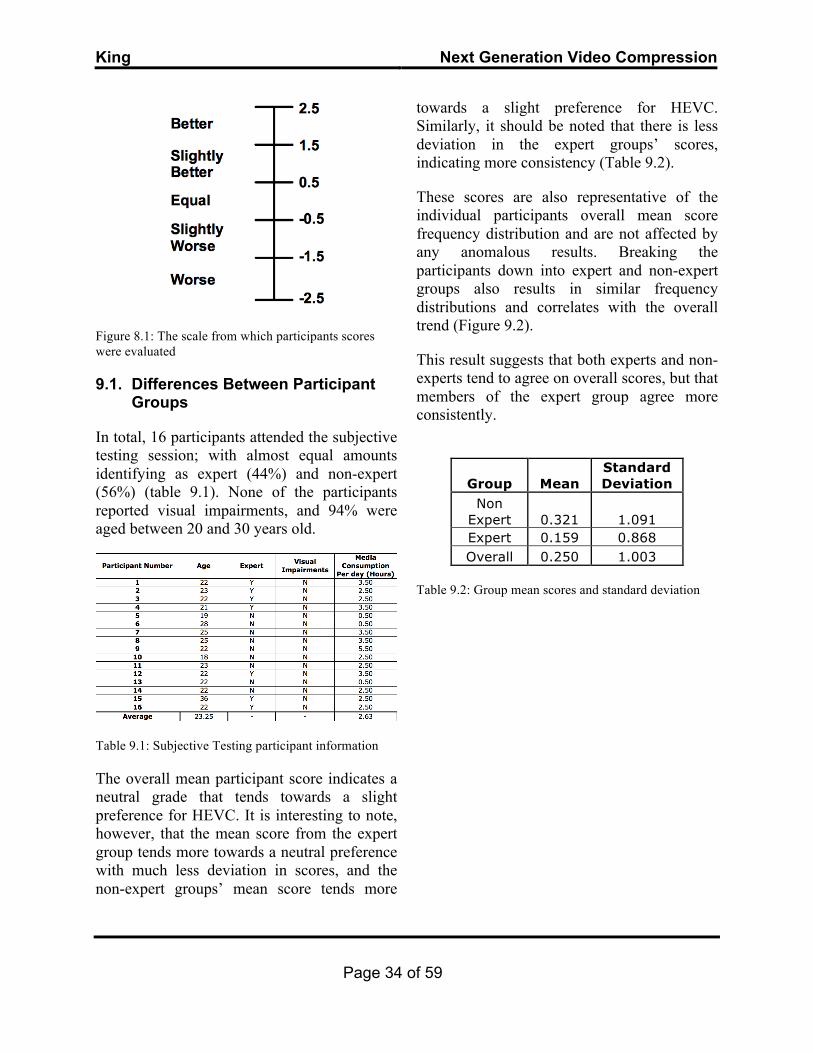
For all data in this section, the scores were read from the scale using the scale in figure 8.1. For example a score of 0 indicates that the participant felt that the video quality of the second video was equal to the first, and a score of 1.7 indicates that the participant felt the second video was better than the first etc.
King Next Generation Video Compression
Page 34 of 59
Figure 8.1: The scale from which participants scores were evaluated
9.1. Differences Between Participant Groups
In total, 16 participants attended the subjective testing session; with almost equal amounts identifying as expert (44%) and non-expert (56%) (table 9.1). None of the participants reported visual impairments, and 94% were aged between 20 and 30 years old.
Table 9.1: Subjective Testing participant information
The overall mean participant score indicates a neutral grade that tends towards a slight preference for HEVC. It is interesting to note, however, that the mean score from the expert group tends more towards a neutral preference with much less deviation in scores, and the non-expert groups’ mean score tends more
towards a slight preference for HEVC. Similarly, it should be noted that there is less deviation in the expert groups’ scores, indicating more consistency (Table 9.2).
These scores are also representative of the individual participants overall mean score frequency distribution and are not affected by any anomalous results. Breaking the participants down into expert and non-expert groups also results in similar frequency distributions and correlates with the overall trend (Figure 9.2).
This result suggests that both experts and non-experts tend to agree on overall scores, but that members of the expert group agree more consistently.
Group Mean Standard Deviation
Non Expert 0.321 1.091 Expert 0.159 0.868 Overall 0.250 1.003
Table 9.2: Group mean scores and standard deviation
King Next Generation Video Compression
Page 35 of 59
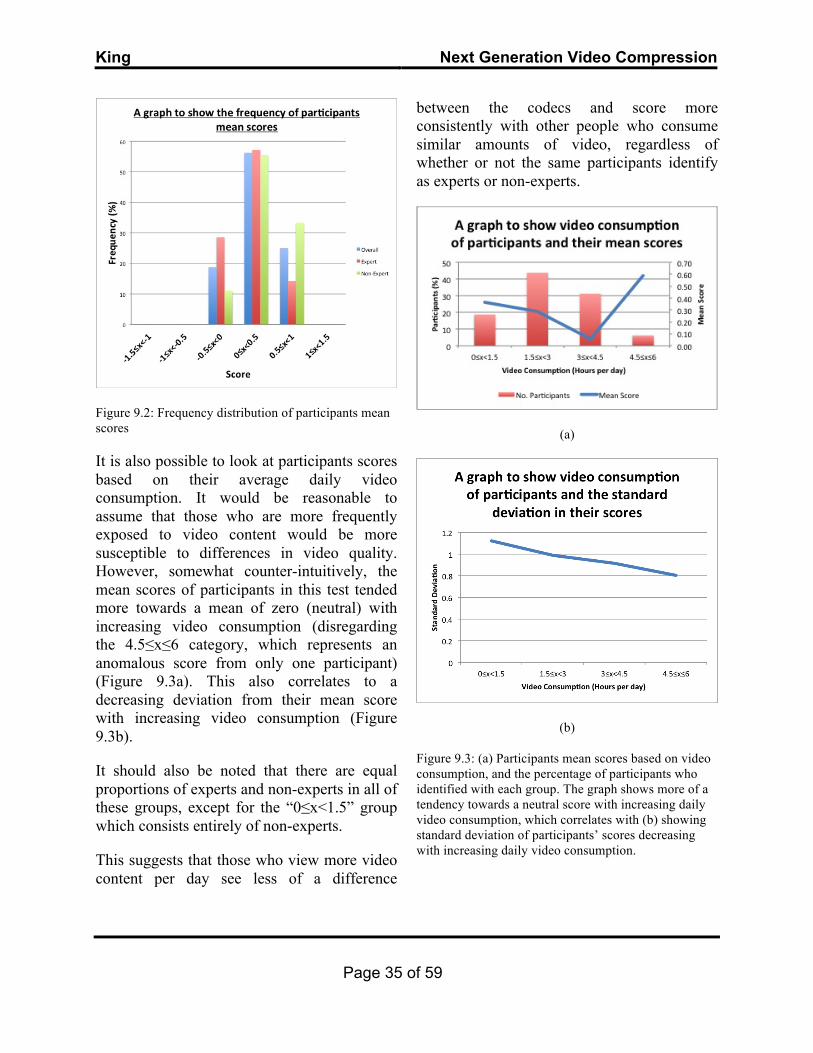
Figure 9.2: Frequency distribution of participants mean scores
It is also possible to look at participants scores based on their average daily video consumption. It would be reasonable to assume that those who are more frequently exposed to video content would be more susceptible to differences in video quality. However, somewhat counter-intuitively, the mean scores of participants in this test tended more towards a mean of zero (neutral) with increasing video consumption (disregarding the 4.5≤x≤6 category, which represents an anomalous score from only one participant) (Figure 9.3a). This also correlates to a decreasing deviation from their mean score with increasing video consumption (Figure 9.3b).
It should also be noted that there are equal proportions of experts and non-experts in all of these groups, except for the “0≤x<1.5” group which consists entirely of non-experts.
This suggests that those who view more video content per day see less of a difference
between the codecs and score more consistently with other people who consume similar amounts of video, regardless of whether or not the same participants identify as experts or non-experts.
(a)
(b)
Figure 9.3: (a) Participants mean scores based on video consumption, and the percentage of participants who identified with each group. The graph shows more of a tendency towards a neutral score with increasing daily video consumption, which correlates with (b) showing standard deviation of participants’ scores decreasing with increasing daily video consumption.
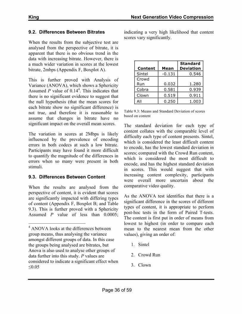
King Next Generation Video Compression
Page 36 of 59
9.2. Differences Between Bitrates
When the results from the subjective test are analysed from the perspective of bitrate, it is apparent that there is no obvious trend in the data with increasing bitrate. However, there is a much wider variation in scores at the lowest bitrate, 2mbps (Appendix F, Boxplot A).
This is further proved with Analysis of Variance (ANOVA), which shows a Sphericity Assumed P value of 0.144. This indicates that there is no significant evidence to suggest that the null hypothesis (that the mean scores for each bitrate show no significant difference) is not true, and therefore it is reasonable to assume that changes in bitrate have no significant impact on the overall mean scores.
The variation in scores at 2Mbps is likely influenced by the prevalence of encoding errors in both codecs at such a low bitrate. Participants may have found it more difficult to quantify the magnitude of the differences in errors when so many were present in both stimuli.
9.3. Differences Between Content
When the results are analysed from the perspective of content, it is evident that scores are significantly impacted with differing types of content (Appendix F, Boxplot B; and Table 9.3). This is further proved with a Sphericity Assumed P value of less than 0.0005;
4 ANOVA looks at the differences between group means, thus analysing the variance amongst different groups of data. In this case the groups being analysed are bitrates, but Anova is also used to analyse other groups of data further into this study. P values are considered to indicate a significant effect when ≤0.05
indicating a very high likelihood that content scores vary significantly.
Content Mean Standard Deviation
Sintel -0.131 0.546 Crowd Run 0.032 1.280 Cobra 0.581 0.939 Clown 0.519 0.911 All 0.250 1.003
Table 9.3: Means and Standard Deviation of scores based on content
The standard deviation for each type of content collates with the comparable level of difficulty each type of content presents. Sintel, which is considered the least difficult content to encode, has the lowest standard deviation in scores; compared with the Crowd Run content, which is considered the most difficult to encode, and has the highest standard deviation in scores. This would suggest that with increasing content complexity, participants were overall more uncertain about the comparative video quality.
As the ANOVA test identifies that there is a significant difference in the scores of different types of content, it is appropriate to perform post-hoc tests in the form of Paired T-tests. The content is first put in order of means from lowest to highest (in order to compare each mean to the nearest mean from the other values), giving an order of:
1. Sintel
2. Crowd Run
3. Clown
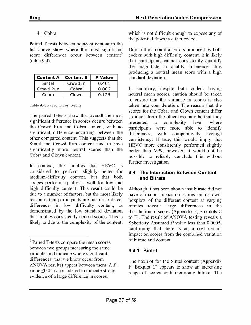
King Next Generation Video Compression
Page 37 of 59
4. Cobra
Paired T-tests between adjacent content in the list above show where the most significant score differences occur between content5 (table 9.4).
Content A Content B P Value
Sintel Crowdun 0.401 Crowd Run Cobra 0.006
Cobra Clown 0.126
Table 9.4: Paired T-Test results
The paired T-tests show that overall the most significant difference in scores occurs between the Crowd Run and Cobra content, with no significant difference occurring between the other compared content. This suggests that the Sintel and Crowd Run content tend to have significantly more neutral scores than the Cobra and Clown content.
In context, this implies that HEVC is considered to perform slightly better for medium-difficulty content, but that both codecs perform equally as well for low and high difficulty content. This result could be due to a number of factors, but the most likely reason is that participants are unable to detect differences in low difficulty content, as demonstrated by the low standard deviation that implies consistently neutral scores. This is likely to due to the complexity of the content,
5 Paired T-tests compare the mean scores between two groups measuring the same variable, and indicate where significant differences (that we know occur from ANOVA results) appear between them. A P value ≤0.05 is considered to indicate strong evidence of a large difference in scores.
which is not difficult enough to expose any of the potential flaws in either codec.
Due to the amount of errors produced by both codecs with high difficulty content, it is likely that participants cannot consistently quantify the magnitude in quality difference, thus producing a neutral mean score with a high standard deviation.
In summary, despite both codecs having neutral mean scores, caution should be taken to ensure that the variance in scores is also taken into consideration. The reason that the scores for the Cobra and Clown content differ so much from the other two may be that they presented a complexity level where participants were more able to identify differences, with comparatively average consistency. If true, this would imply that HEVC more consistently performed slightly better than VP9, however, it would not be possible to reliably conclude this without further investigation.
9.4. The Interaction Between Content and Bitrate
Although it has been shown that bitrate did not have a major impact on scores on its own, boxplots of the different content at varying bitrates reveals large differences in the distribution of scores (Appendix F, Boxplots C to F). The result of ANOVA testing reveals a Sphericity Assumed P value less than 0.0005, confirming that there is an almost certain impact on scores from the combined variation of bitrate and content.
9.4.1. Sintel
The boxplot for the Sintel content (Appendix F, Boxplot C) appears to show an increasing range of scores with increasing bitrate. The
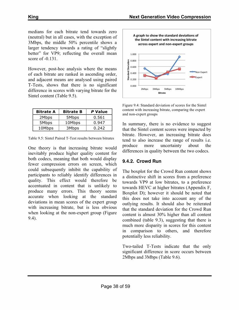
King Next Generation Video Compression
Page 38 of 59
medians for each bitrate tend towards zero (neutral) but in all cases, with the exception of 3Mbps, the middle 50% percentile shows a larger tendency towards a rating of “slightly better” for VP9; reflecting the overall mean score of -0.131.
However, post-hoc analysis where the means of each bitrate are ranked in ascending order, and adjacent means are analysed using paired T-Tests, shows that there is no significant difference in scores with varying bitrate for the Sintel content (Table 9.5).
Bitrate A Bitrate B P Value
2Mbps 5Mbps 0.561 5Mbps 10Mbps 0.947 10Mbps 3Mbps 0.242
Table 9.5: Sintel Paired T-Test results between bitrates
One theory is that increasing bitrate would inevitably produce higher quality content for both codecs, meaning that both would display fewer compression errors on screen, which could subsequently inhibit the capability of participants to reliably identify differences in quality. This effect would therefore be accentuated in content that is unlikely to produce many errors. This theory seems accurate when looking at the standard deviations in mean scores of the expert group with increasing bitrate, but is less obvious when looking at the non-expert group (Figure 9.4).
Figure 9.4: Standard deviation of scores for the Sintel content with increasing bitrate, comparing the expert and non-expert groups
In summary, there is no evidence to suggest that the Sintel content scores were impacted by bitrate. However, an increasing bitrate does tend to also increase the range of results i.e. produce more uncertainty about the differences in quality between the two codecs.
9.4.2. Crowd Run
The boxplot for the Crowd Run content shows a distinctive shift in scores from a preference towards VP9 at low bitrates, to a preference towards HEVC at higher bitrates (Appendix F, Boxplot D); however it should be noted that this does not take into account any of the outlying results. It should also be reiterated that the standard deviation for the Crowd Run content is almost 30% higher than all content combined (table 9.3), suggesting that there is much more disparity in scores for this content in comparison to others, and therefore potentially less reliability.
Two-tailed T-Tests indicate that the only significant difference in score occurs between 2Mbps and 3Mbps (Table 9.6).
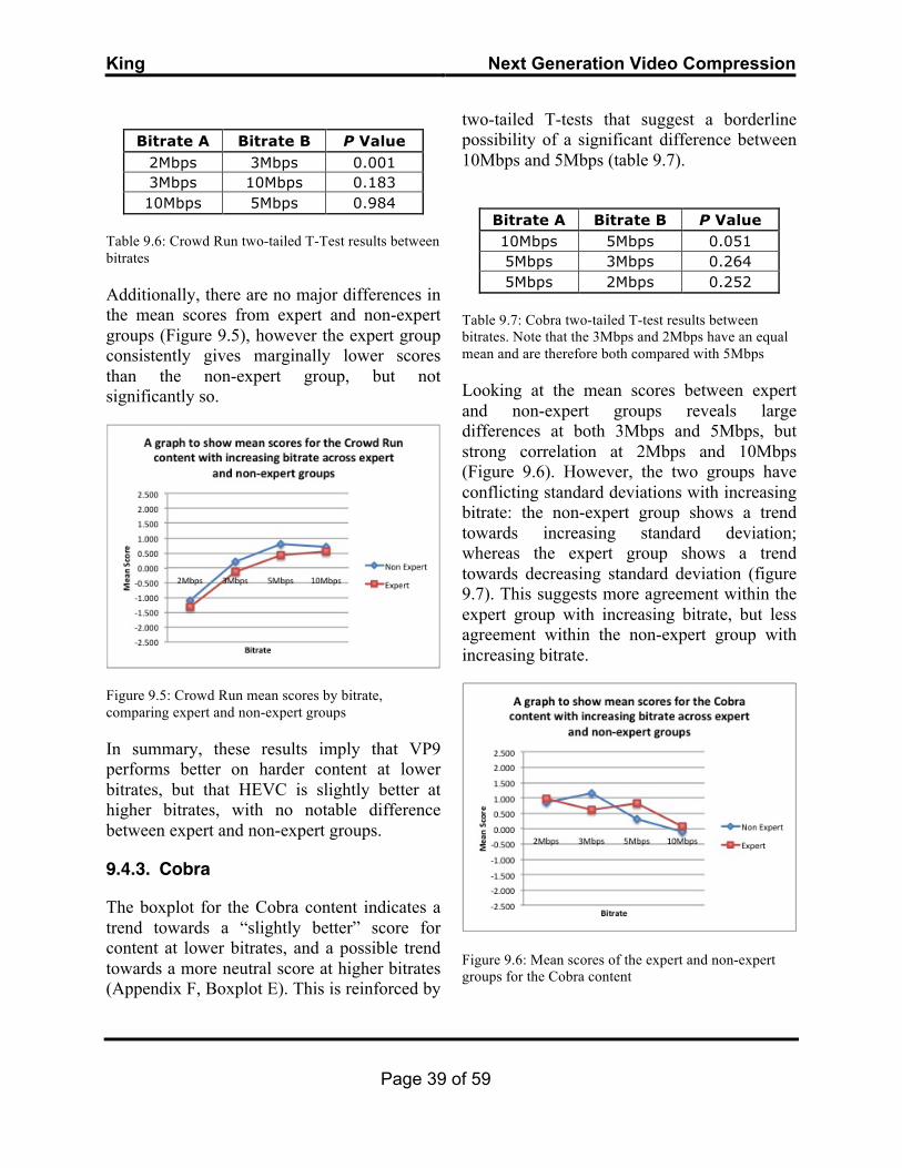
King Next Generation Video Compression
Page 39 of 59
Bitrate A Bitrate B P Value
2Mbps 3Mbps 0.001 3Mbps 10Mbps 0.183 10Mbps 5Mbps 0.984
Table 9.6: Crowd Run two-tailed T-Test results between bitrates
Additionally, there are no major differences in the mean scores from expert and non-expert groups (Figure 9.5), however the expert group consistently gives marginally lower scores than the non-expert group, but not significantly so.
Figure 9.5: Crowd Run mean scores by bitrate, comparing expert and non-expert groups
In summary, these results imply that VP9 performs better on harder content at lower bitrates, but that HEVC is slightly better at higher bitrates, with no notable difference between expert and non-expert groups.
9.4.3. Cobra
The boxplot for the Cobra content indicates a trend towards a “slightly better” score for content at lower bitrates, and a possible trend towards a more neutral score at higher bitrates (Appendix F, Boxplot E). This is reinforced by
two-tailed T-tests that suggest a borderline possibility of a significant difference between 10Mbps and 5Mbps (table 9.7).
Bitrate A Bitrate B P Value 10Mbps 5Mbps 0.051 5Mbps 3Mbps 0.264 5Mbps 2Mbps 0.252
Table 9.7: Cobra two-tailed T-test results between bitrates. Note that the 3Mbps and 2Mbps have an equal mean and are therefore both compared with 5Mbps
Looking at the mean scores between expert and non-expert groups reveals large differences at both 3Mbps and 5Mbps, but strong correlation at 2Mbps and 10Mbps (Figure 9.6). However, the two groups have conflicting standard deviations with increasing bitrate: the non-expert group shows a trend towards increasing standard deviation; whereas the expert group shows a trend towards decreasing standard deviation (figure 9.7). This suggests more agreement within the expert group with increasing bitrate, but less agreement within the non-expert group with increasing bitrate.
Figure 9.6: Mean scores of the expert and non-expert groups for the Cobra content
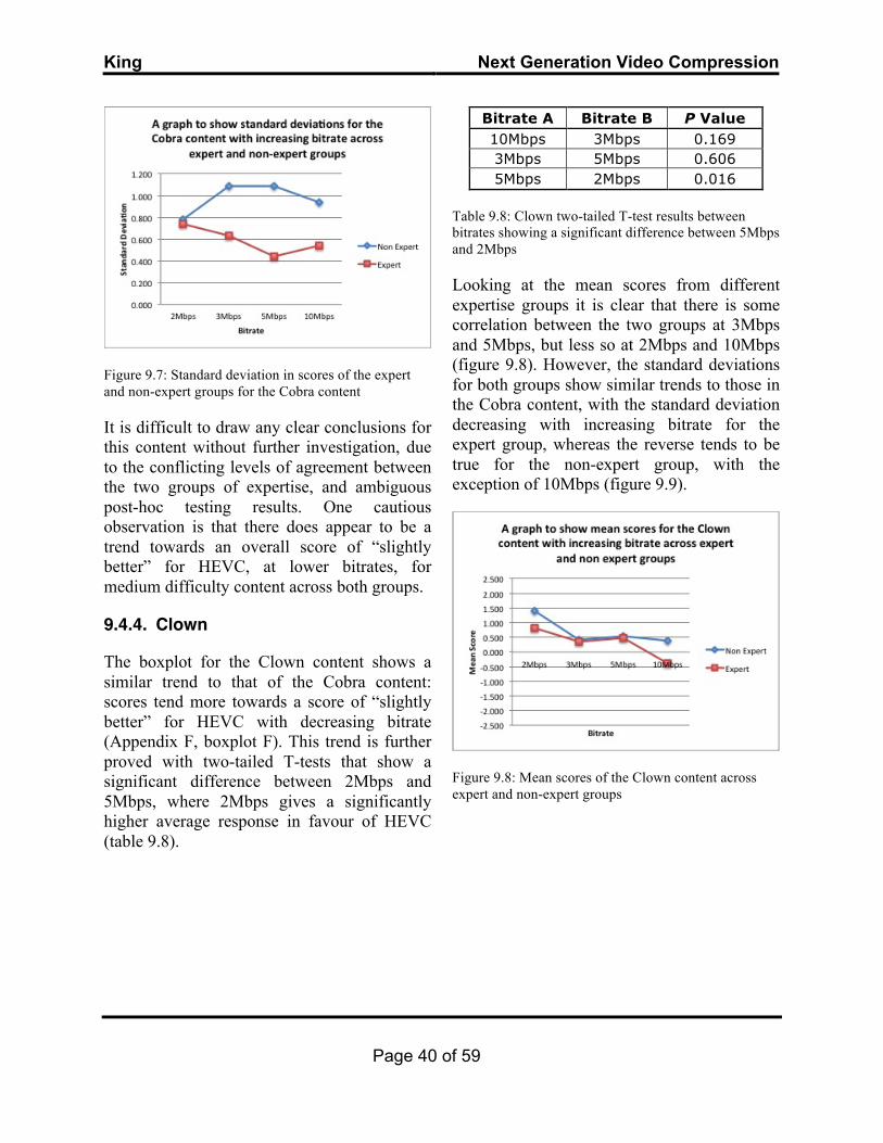
King Next Generation Video Compression
Page 40 of 59
Figure 9.7: Standard deviation in scores of the expert and non-expert groups for the Cobra content
It is difficult to draw any clear conclusions for this content without further investigation, due to the conflicting levels of agreement between the two groups of expertise, and ambiguous post-hoc testing results. One cautious observation is that there does appear to be a trend towards an overall score of “slightly better” for HEVC, at lower bitrates, for medium difficulty content across both groups.
9.4.4. Clown
The boxplot for the Clown content shows a similar trend to that of the Cobra content: scores tend more towards a score of “slightly better” for HEVC with decreasing bitrate (Appendix F, boxplot F). This trend is further proved with two-tailed T-tests that show a significant difference between 2Mbps and 5Mbps, where 2Mbps gives a significantly higher average response in favour of HEVC (table 9.8).
Bitrate A Bitrate B P Value 10Mbps 3Mbps 0.169 3Mbps 5Mbps 0.606 5Mbps 2Mbps 0.016
Table 9.8: Clown two-tailed T-test results between bitrates showing a significant difference between 5Mbps and 2Mbps
Looking at the mean scores from different expertise groups it is clear that there is some correlation between the two groups at 3Mbps and 5Mbps, but less so at 2Mbps and 10Mbps (figure 9.8). However, the standard deviations for both groups show similar trends to those in the Cobra content, with the standard deviation decreasing with increasing bitrate for the expert group, whereas the reverse tends to be true for the non-expert group, with the exception of 10Mbps (figure 9.9).
Figure 9.8: Mean scores of the Clown content across expert and non-expert groups
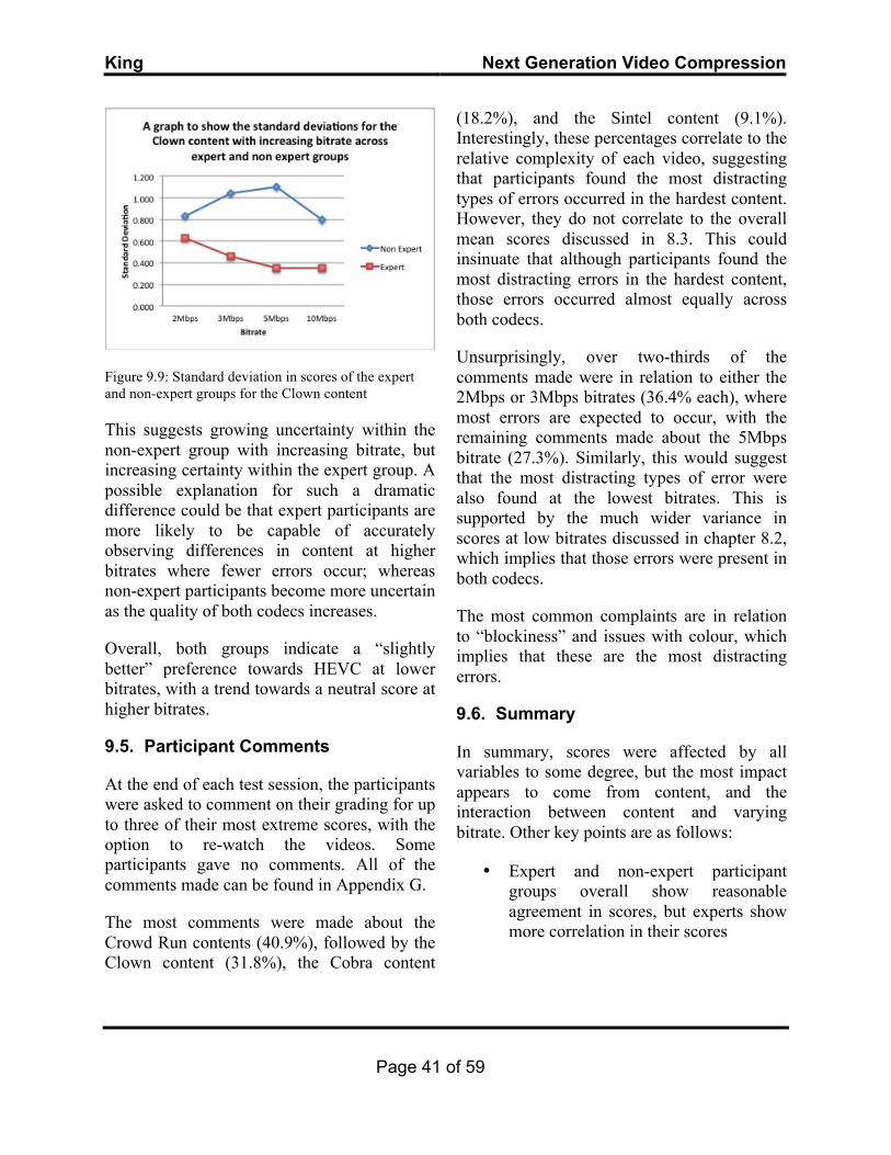
King Next Generation Video Compression
Page 41 of 59
Figure 9.9: Standard deviation in scores of the expert and non-expert groups for the Clown content
This suggests growing uncertainty within the non-expert group with increasing bitrate, but increasing certainty within the expert group. A possible explanation for such a dramatic difference could be that expert participants are more likely to be capable of accurately observing differences in content at higher bitrates where fewer errors occur; whereas non-expert participants become more uncertain as the quality of both codecs increases.
Overall, both groups indicate a “slightly better” preference towards HEVC at lower bitrates, with a trend towards a neutral score at higher bitrates.
9.5. Participant Comments
At the end of each test session, the participants were asked to comment on their grading for up to three of their most extreme scores, with the option to re-watch the videos. Some participants gave no comments. All of the comments made can be found in Appendix G.
The most comments were made about the Crowd Run contents (40.9%), followed by the Clown content (31.8%), the Cobra content
(18.2%), and the Sintel content (9.1%). Interestingly, these percentages correlate to the relative complexity of each video, suggesting that participants found the most distracting types of errors occurred in the hardest content. However, they do not correlate to the overall mean scores discussed in 8.3. This could insinuate that although participants found the most distracting errors in the hardest content, those errors occurred almost equally across both codecs.
Unsurprisingly, over two-thirds of the comments made were in relation to either the 2Mbps or 3Mbps bitrates (36.4% each), where most errors are expected to occur, with the remaining comments made about the 5Mbps bitrate (27.3%). Similarly, this would suggest that the most distracting types of error were also found at the lowest bitrates. This is supported by the much wider variance in scores at low bitrates discussed in chapter 8.2, which implies that those errors were present in both codecs.
The most common complaints are in relation to “blockiness” and issues with colour, which implies that these are the most distracting errors.
9.6. Summary
In summary, scores were affected by all variables to some degree, but the most impact appears to come from content, and the interaction between content and varying bitrate. Other key points are as follows:
• Expert and non-expert participant groups overall show reasonable agreement in scores, but experts show more correlation in their scores

King Next Generation Video Compression
Page 42 of 59
• Participants who watch more video content per day are less likely to see differences between the two codecs
• Bitrate alone shows no significant impact on scores
• There is strong evidence to suggest that content, and varying bitrate within content, has the most substantial impact on scores
• Participants comments suggest that the most distracting errors are colour issues and “blockiness”
10. CONCLUSION
Looking at the features they employ it is clear that both codecs have been appropriately developed with current consumer level hardware in mind, where increasing power and number of processor cores available allow decoding devices to handle greater complexity and parallelisation. An increase in the complexity of each codec and the advanced parallelisation tools that play such a major part in them both shows a clear progression from previous standards. HEVC demonstrates advancements upon its predecessor AVC in the form of refining its features to make them more complex and more efficient, as well as implementing completely new features such as WPP and a new quadtree coding structure; VP9, despite being the newcomer to the compression industry, introduces new techniques such as ARFs and ADST transforms, without access to patents that would have previously been considered essential, and has done so largely through open-source community development.
The subjective testing conducted in this study shows very little difference between the codecs, with the overall score laying within the “equal” bracket of measurement. However, there are differences between the codecs on differing content, where HEVC produces a score of “slightly better” for medium-difficulty content in comparison to VP9, but both codecs perform equally for low and high complexity content. Looking closer at the relationship between bitrate and content, HEVC shows a much clearer advantage at lower bitrates for medium-difficulty content, but there is a trend towards a more neutral score with increasing bitrate. On the contrary, VP9 shows more of an advantage for high-difficulty content at low bitrates, but loses preference to HEVC with increasing bitrate.
Unsurprisingly, participants who identify as experts show more correlation in their scores, and are therefore perhaps more reliable, however, the overall trend for non-experts tends to follow the same pattern. This is an important result as it confirms that non-expert consumers, who will make up the vast majority of the target market, see differences between the codecs in some areas which could influence the decision of which codec vendors are likely to use depending on the content they are producing and the bitrate they are distributing it at.
The results of these subjective tests, therefore, largely mirrors those of other comparative tests between the codecs in that there is no conclusive evidence to suggest an overall advantage of either codec.
It is likely then that one of the largest influences on vendors to choose either codec will ultimately be a financial one. However, the strong reputation and rich history of HEVC’s predecessors may give it an
King Next Generation Video Compression
Page 43 of 59
advantage over VP9, which, realistically, will need to prove its reliability and practicality in the near future in order to become a viable competitor.
11. FURTHER WORK
This study compared the encoders using medium-complexity settings, it would be beneficial to see the differences between the codecs when they are both using their best, and most complex, settings. However, to be at all viable, much more powerful equipment would be needed for the encoding and decoding processes. Similarly, more powerful hardware would allow for a comparison between compressed and uncompressed video, which would produce more credible results.
Alternatively, it would also be beneficial to see how each codec performs using low complexity profiles designed for the streaming of video to mobile devices, where a decrease in bitrates represents a more direct decrease in cost to the consumer.
Finally, another study, when both codecs have been fully ratified, and their documentation fully released, will allow for a more transparent comparison and give a greater indication of the advantages of each.

King Next Generation Video Compression
Page 44 of 59
12. REFERENCES Benoit. H. (2002). Digital Television: MPEG-1, MPEG-2 and principles of the DVB system. Focal Press.
British Standards Institute (1993). Coding of moving pictures and associated audio for digital storage at up to about 1.5 Mbit/s – Part 2: Video. (BS EN ISO/IEC 11172-2).
Chi, C., Alvarez-Mesa, M., Juurlink, B., Clare, G., Henry, F., Pateux, S., and Schierl, T. (2012). Parallel Scalability and Efficiency of HEVC Parallelization Approaches. IEEE Transactions on Circuits and Systems for Video Technology, Vol. 22 (12), P.1827-1838. DOI: 10.1109/TCSVT.2012.2223056
Cornsweet, T.N. (1970). Visual Perception. Academic Press Inc. Davson, H. (1980). Physiology of the Eye (4th ed.). Palgrave Macmillan
Delargy, J., Wendt, P.(1996). A performance comparison of three software video codecs for IBM RISC System/6000 workstations. Signal Processing-image Communication, Vol.8(1), 39-44. doi:10.1016/0923-5965(95)00015-1 Digital Video Broadcasting (DVB) (2014). Specification for the use of Video and Audio coding in Broadcasting Applications based on the MPEG-2 Transport Stream. (DVB Document A157). Retrieved from https://www.dvb.org/resources/public/standards/a157_dvb-avc-mpeg2.pdf
Ferguson, T. (2001). Retrieved 2014, 3rd November from http://multimedia.cx/mirror/cinepak.txt Ffmpeg. (n.d). H.265 Encoding Guide. Retrieved April 2015 from https://trac.ffmpeg.org/wiki/Encode/H.265 Ghanbari, M. (1999), Video Coding, IEEE
Ghanbari, M. (2011). Standard Codecs: Image Compression to Advanced Video Coding (3rd Ed.). IEE.
Grange, A., Alvestrand, H. (2013). A VP9 Bitstream Overview. Google. Grois, D., Marpe, D., Mulayoff, A., and Hadar, O. (2013). Performance Comparison of H.265/MPEG-HEVC, VP9, and H.264/MPEG-AVC Encoders. 2013 Picture Coding Symposium, P.394-7. doi:10.1109/PCS.2013.6737766
Hardy, A.C. (1919). An Experimental Study of the Persistence of Vision Heo, J., Kim, S., Ho, Y. (2010). Improved CAVLC for H.264/AVC Lossless Intra Coding. IEEE Transactions on Circuits and Systems for Video Technology, Vol. 20(2), 213-222. DOI: 10.1109/TCSVT.2009.2031392
Ibrahim, K.F.(2007), Newnes guide to Television & Video Technology (4th Ed.), Newnes

King Next Generation Video Compression
Page 45 of 59
International Telecommunications Union (ITU) (1988). Video Codec for Audiovisual services at Px64 Kbits. (ITU-T Rec. H.261)
International Telecommunications Union (ITU) (1995). Generic Coding of Moving Pictures and Associated Audio Information: Video. (ITU-T Rec. H.262)
International Telecommunications Union (ITU) (2012). Methodology for the Subjective Assessment of the Quality of Television Pictures. (ITU-R BT.500-13).
International Telecommunications Union (ITU) (2013). Advanced Video Coding for Generic Audiovisual Services (8th Ed.). (ITU-T Rec. H.264)
Ishihara, S. (1917). Test for Colour-Blindness Kapsenberg, P. (2013). How VP9 works, technical details, and diagrams. Retrieved from http://forum.doom9.org/showthread.php?t=168947 Landis, C. (1954). Determinants of the Critical Flicker-Fusion Threshold
Mathematicalmonk. (2011). Arithmetic Coding - Example #1. [Online Video]. 08 October 2011. Retrieved from: https://www.youtube.com/watch?v=7vfqhoJVwuc. Accessed: 01 December 2014. Misra, K., Segall, A., Horowitz, M., Xu, S., Fuldseth, A., Zhou, M. (2013). An Overview of Tiles in HEVC. IEEE Journal of Selected Topics in Signal Processing, Vol. 7 (6), 969-977. DOI: 10.1109/JSTSP.2013.2271451
Mukherjee, D., Bankoski, J., Grange, A., Han, J., Koleszar, J., Wilkins, P., Xu, Y., Bultje, R. (2013). The Latest open-source video codec VP9 – An overview and preliminary results. 2013 Picture Coding Symposium, P.390-93. DOI: 10.1109/PCS.2013.6737765 Panasonic. (n.d). Specification for Panasonic TX-58AX802B. Retrieved April 28th 2015 from http://www.panasonic.com/uk/consumer/viera-televisions/led/tx-58ax802b.specs.html Ramamoorthy, R (Google Developers, 2014, June 25th). Update on WebM/VP9. Retrieved from https://www.youtube.com/watch?v=xo_R40C7RTo Remington, L.A. (2012). Clinical Anatomy and Physiology of the Visual System (3rd ed.). Butterworth-Heinemann Rerabek, M. and Ebrahimi, T. (2014). Comparison of compression efficiency between HEVC/H.265 and VP9 based on subjective assessments. Applications of Digital Image Processing, Vol. 9217. doi:10.1117/12.2065561.
Richardson, I.E.G (2003), H.264 and MPEG-4 – Video Coding for Next-generation Multimedia. Wiley.
Seabrook, G.R.(1989). Arithmetic Coding – An alternative VLC strategy for video coding. Third International Conference on Image Processing and its Applications, P.613-17. IET.
Segaretro (2014), Retrieved 2014, 3rd November from http://segaretro.org/Cinepak
King Next Generation Video Compression
Page 46 of 59
Sullivan, G.J., Ohm, J., Han, W., Wiegand, T. (2012). An Overview of the High Efficiency Video Coding (HEVC) Standard. IEEE Transactions on Circuits and Systems for Video Technology, Vol. 22 (12), 1649-68. DOI: 10.1109/TCSVT.2012.2221191 The Webm Project. (n.d.) Encoder Parameters. Retrieved April 1st 2015 from http://wiki.webmproject.org/ffmpeg/vp9-encoding-guide The Webm Project. (n.d.). Retrieved March 31st, 2015 from http://www.webmproject.org/about/faq/ Watkinson, J.(2004) The MPEG Handbook (2nd ed.), Elsevier
Watkinson, J.(2008), The Art of Digital Video 4th Edition, John Watkinson, Focal Press Wilkins, P. (8th May 2013). VP9 Bitstream finalization update. WebM Project. Google.
X265. (n.d). X265 Preset Options. Retrieved April 2015 from http://x265.readthedocs.org/en/default/presets.htm
Zhang, S., Zhang, X., Gao, Z. (2014). Implementation and improvement of Wavefront Parallel Processing for HEVC encoding on many-core platform. Presented at IEEE International Conference on Multimedia and Expo. DOI: 10.1109/ICMEW.2014.6890596

King Next Generation Video Compression
Page 47 of 59
Appendix A: Table of defined MPEG-2 Profiles and Levels
Profiles
Simple Main 4:2:2 SNR Spatial High
Levels
High 4:2:0
1920x1152 90Mb/s
4:2:0 or 4:2:2
1920x1152 100Mb/s
High 1440
4:2:0
1440x1152 60Mb/s
4:2:0
1440x1152 60Mb/s
4:2:0 or 4:2:2
1440x1152 80Mb/s
Main 4:2:0
720x576 15Mb/s No B
4:2:0 720x576 15Mb/s
4:2:2 720x608 50Mb/s
4:2:0 720x576 15Mb/s
4:2:0 or 4:2:2
720x576 20Mb/s
Low 4:2:0
352x288 4Mb/s
4:2:0
352x288 4Mb/s
Appendix B: Table of maximum number of enhancement layers for each MPEG-2 scalable profile (International Telecommunications Union, 1995)
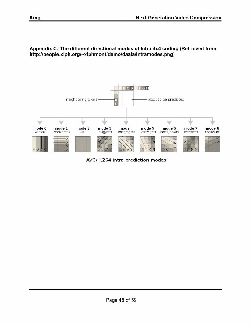
King Next Generation Video Compression
Page 48 of 59
Appendix C: The different directional modes of Intra 4x4 coding (Retrieved from http://people.xiph.org/~xiphmont/demo/daala/intramodes.png)

King Next Generation Video Compression
Page 49 of 59
Appendix D: HEVC picture partitioning compared with H.264 picture partitioning
Appendix E: Subjective Testing Encoder Commands
VP9: ffmpeg -y -i <input> -c:v libvpx-vp9 -pass 1 -b:v <bitrate> -deadline good -speed 4 -tile-columns 6 -frame-parallel 1 -auto-alt-ref 1 -rc_lookahead 25 -g 250 -keyint_min 25 -arnr_max_frames 7 -arnr_strength 5 -an -f webm /dev/null && ffmpeg -y -i <Input> -c:v libvpx-vp9 -pass 2 -b:v <Bitrate> -deadline good -speed 2 -tile-columns 6 -frame-parallel 1 -auto-alt-ref 1 -rc_lookahead 25 -g 250 -keyint_min 25 -arnr_max_frames 7 -arnr_strength 5 -an -f webm <output>.webm
HEVC:
ffmpeg -y -i <input> -c:v hevc -pass 1 -x265-params ref=4:bframes=16:b-adapt=2 -b:v <bitrate> -preset medium -pix_fmt yuv420p -f mp4 /dev/null && ffmpeg -y -i <input> -c:v hevc -pass 2 -x265-params ref=4:bframes=16:b-adapt=2 -b:v <bitrate> -preset medium -pix_fmt yuv420p -f mp4 <output>.mp4
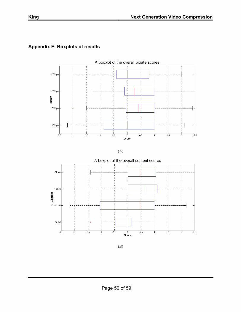
King Next Generation Video Compression
Page 50 of 59
Appendix F: Boxplots of results
(A)
(B)

King Next Generation Video Compression
Page 51 of 59
(C)
(D)

King Next Generation Video Compression
Page 52 of 59
(E)
(F)

King Next Generation Video Compression
Page 53 of 59
Appendix G: Test Participants Comments

King Next Generation Video Compression
Page 54 of 59
Glossary of Important Terms and Equations
Progressive and Interlaced scanning
These are the two scanning methods used by televisions to reproduce video.
Interlaced scanning is a scanning method inherited from analogue where each frame is split into two fields. The first field contains all of the information for the odd horizontal lines, and the second field contains the information for the even horizontal lines. The two fields are displayed in quick succession to show the full frame. This system was used in analogue to save bandwidth, as only half the data rate needed to display the equivalent video scanned progressively, is required.
Progressive scanning is a scanning method where the entire frame is displayed at once. This is generally preferred to interlaced scanning, in terms of quality, as it does not produce the same artefacts on the screen that are sometimes seen with interlaced scanning for video with fast moving action.
Lossless and Lossy Compression
Lossless compression reproduces identical data at the output of the decoder, to what was seen at the input of the encoder. This is done in a variety of ways to ensure that data is stored in the most efficient way possible and all redundant data is removed.
Lossless compression methods cannot guarantee a particular compression ratio as it depends how much redundant information is
present. However, in general, lossless compression is limited to a compression ratio of around 2:1 (Watkinson, 2004).
Lossy compression will not reproduce identical data at the decoder to that seen at the input of the encoder. Lossy compression methods introduce errors into the data stream and try to arrange them, using psychovisual techniques, so that they are as unperceivable as possible to the viewer. This type of compression offers much higher compression ratios and is used in most broadcast applications.
Sampling
The eye is more sensitive to green than it is to red and blue, therefore samples in a video signal are taken of chrominance red (Cr) and chrominance blue (Cb); with the green portion being calculated by subtracting the Cr and Cb values from the Y value. This is so that the lowest amount of data possible can be used to store the full luminance and chrominance data of the image. The resulting signal is commonly written as YCrCb, but in digital video is also sometimes referred to as YUV.
When video is recorded or displayed, the luminance and chrominance (colour) samples are not recorded in equal proportions, as the eye is more sensitive to changes in luminance, therefore there are various sample rates that can be used to carry colour information in varying degrees of accuracy.
The most common sampling rates are 4:2:2 and 4:2:0.
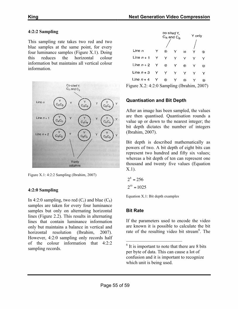
King Next Generation Video Compression
Page 55 of 59
4:2:2 Sampling
This sampling rate takes two red and two blue samples at the same point, for every four luminance samples (Figure X.1). Doing this reduces the horizontal colour information but maintains all vertical colour information.
Figure X.1: 4:2:2 Sampling (Ibrahim, 2007)
4:2:0 Sampling
In 4:2:0 sampling, two red (Cr) and blue (Cb) samples are taken for every four luminance samples but only on alternating horizontal lines (Figure 2.2). This results in alternating lines that contain luminance information only but maintains a balance in vertical and horizontal resolution (Ibrahim, 2007). However, 4:2:0 sampling only records half of the colour information that 4:2:2 sampling records.
Figure X.2: 4:2:0 Sampling (Ibrahim, 2007)
Quantisation and Bit Depth
After an image has been sampled, the values are then quantised. Quantisation rounds a value up or down to the nearest integer; the bit depth dictates the number of integers (Ibrahim, 2007).
Bit depth is described mathematically as powers of two. A bit depth of eight bits can represent two hundred and fifty six values; whereas a bit depth of ten can represent one thousand and twenty five values (Equation X.1).
Equation X.1: Bit depth examples
Bit Rate
If the parameters used to encode the video are known it is possible to calculate the bit rate of the resulting video bit stream6. The
6 It is important to note that there are 8 bits per byte of data. This can cause a lot of confusion and it is important to recognize which unit is being used.
€
28 = 256210 =1025
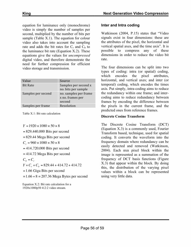
King Next Generation Video Compression
Page 56 of 59
equation for luminance only (monochrome) video is simply the number of samples per second, multiplied by the number of bits per sample (Table X.1). The equation for colour video also takes into account the sampling rate and adds the bit rates for Cr and Cb to the luminance bit rate (Equation X.2). These equations give the values for uncompressed digital video, and therefore demonstrate the need for further compression for efficient video storage and transmission.
Value Source Bit Rate Samples per second x
no. bits per sample Samples per second no. samples per frame
x no. frames per second
Samples per frame Resolution
Table X.1: Bit rate calculation
Equation X.2: Bit rate calculation for a 1920x1080p50 4:2:2 video stream.
Inter and Intra coding
Watkinson (2004, P.15) states that “Video signals exist in four dimensions: these are the attributes of the pixel, the horizontal and vertical spatial axes, and the time axis”. It is possible to compress any of these dimensions in order to reduce the video bit rate.
The four dimensions can be split into two types of coding: intra (or spatial) coding, which encodes the pixel attributes, horizontal, and vertical axes; and inter (or temporal) coding, which encodes the times axis. Put simply, intra-coding aims to reduce the redundancy within one frame; and inter-coding aims to reduce redundancy between frames by encoding the difference between the pixels in the current frame, and the predicted ones from reference frames. Discrete Cosine Transform
The Discrete Cosine Transform (DCT) (Equation X.3) is a commonly used, Fourier Transform based, technique, used for spatial coding. It converts the waveform into the frequency domain where redundancy can be easily detected and removed (Watkinson, 2004). Each nxn pixel block within the image is represented as a summation of the frequency of DCT basis functions (Figure X.3) that appear within the block. By doing this, the distribution of the varying pixel values within a block can be represented using very little data.
€
Y =1920 ×1080 × 50 × 8= 829,440,000 Bits per second= 829.44 Mega Bits per secondCr = 960 ×1080 × 50 × 8= 414,720,000 Bits per second= 414.72 Mega Bits per secondCb = Cr
Y +Cr +Cb = 829.44 + 414.72 + 414.72=1.66 Giga Bits per second=1.66 ÷ 8 = 207.36 Mega Bytes per second
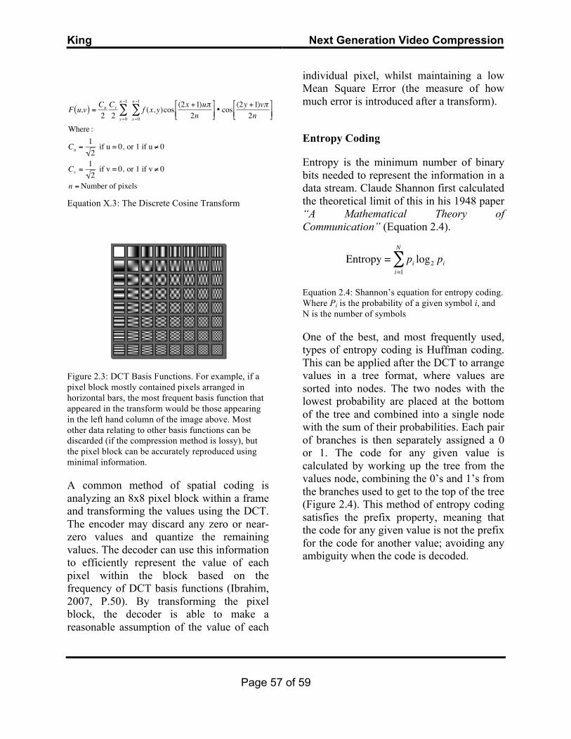
King Next Generation Video Compression
Page 57 of 59
Equation X.3: The Discrete Cosine Transform
Figure 2.3: DCT Basis Functions. For example, if a pixel block mostly contained pixels arranged in horizontal bars, the most frequent basis function that appeared in the transform would be those appearing in the left hand column of the image above. Most other data relating to other basis functions can be discarded (if the compression method is lossy), but the pixel block can be accurately reproduced using minimal information.
A common method of spatial coding is analyzing an 8x8 pixel block within a frame and transforming the values using the DCT. The encoder may discard any zero or near-zero values and quantize the remaining values. The decoder can use this information to efficiently represent the value of each pixel within the block based on the frequency of DCT basis functions (Ibrahim, 2007, P.50). By transforming the pixel block, the decoder is able to make a reasonable assumption of the value of each
individual pixel, whilst maintaining a low Mean Square Error (the measure of how much error is introduced after a transform).
Entropy Coding
Entropy is the minimum number of binary bits needed to represent the information in a data stream. Claude Shannon first calculated the theoretical limit of this in his 1948 paper “A Mathematical Theory of Communication” (Equation 2.4).
Equation 2.4: Shannon’s equation for entropy coding. Where Pi is the probability of a given symbol i, and N is the number of symbols
One of the best, and most frequently used, types of entropy coding is Huffman coding. This can be applied after the DCT to arrange values in a tree format, where values are sorted into nodes. The two nodes with the lowest probability are placed at the bottom of the tree and combined into a single node with the sum of their probabilities. Each pair of branches is then separately assigned a 0 or 1. The code for any given value is calculated by working up the tree from the values node, combining the 0’s and 1’s from the branches used to get to the top of the tree (Figure 2.4). This method of entropy coding satisfies the prefix property, meaning that the code for any given value is not the prefix for the code for another value; avoiding any ambiguity when the code is decoded.
€
F u,v( ) =Cu
2Cv
2 y=0
n−1
∑ f (x,y)cosx=0
n−1
∑ (2x +1)uπ2n
%
& ' (
) * • cos (2y +1)vπ
2n%
& ' (
) *
Where :
Cu =12
if u = 0, or 1 if u ≠ 0
Cv =12
if v = 0, or 1 if v ≠ 0
n = Number of pixels
€
Entropy = pi log2 pii=1
N
∑
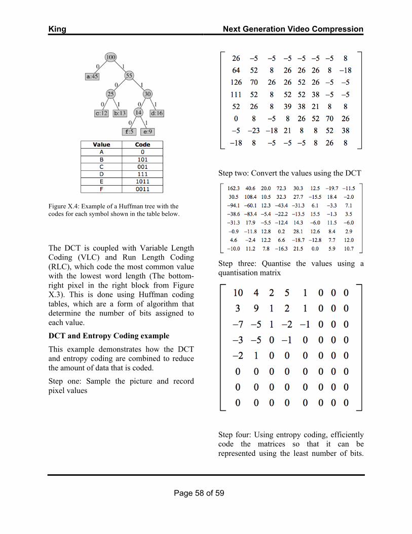
King Next Generation Video Compression
Page 58 of 59
Figure X.4: Example of a Huffman tree with the codes for each symbol shown in the table below.
The DCT is coupled with Variable Length Coding (VLC) and Run Length Coding (RLC), which code the most common value with the lowest word length (The bottom-right pixel in the right block from Figure X.3). This is done using Huffman coding tables, which are a form of algorithm that determine the number of bits assigned to each value. DCT and Entropy Coding example
This example demonstrates how the DCT and entropy coding are combined to reduce the amount of data that is coded. Step one: Sample the picture and record pixel values
Step two: Convert the values using the DCT
Step three: Quantise the values using a quantisation matrix
Step four: Using entropy coding, efficiently code the matrices so that it can be represented using the least number of bits.
King Next Generation Video Compression
Page 59 of 59
Most importantly, this will efficiently encode all of the zero values in the matrix so that they consist of as few bits as possible.
Motion Compensation
Motion compensation is a form of temporal coding that encodes the movement of a pixel, or block of pixels, in the form of a motion vector, between frames so that the decoder can predict its position in the following frame.
Motion compensation is the primary method used for inter-frame compression.