Jack J. Middelburg Marine Carbon Biogeochemistry A Primer ... · roots can be traced back to early scientists documenting how living organisms transformed chemical substances, such

S P R I N G E R B R I E F S I N E A R T H S Y S T E M S C I E N C E S

Jack J. Middelburg

Marine Carbon Biogeochemistry A Primer for Earth System Scientists

SpringerBriefs in Earth System Sciences

Series editors

Gerrit Lohmann, Universität Bremen, Bremen, GermanyLawrence A. Mysak, Department of Atmospheric and Oceanic Sciences, McGillUniversity, Montreal, QC, CanadaJustus Notholt, Institute of Environmental Physics, University of Bremen, Bremen,GermanyJorge Rabassa, Laboratorio de Geomorfología y Cuaternario, CADIC-CONICET,Ushuaia, Tierra del Fuego, ArgentinaVikram Unnithan, Department of Earth and Space Sciences, Jacobs UniversityBremen, Bremen, Germany

SpringerBriefs in Earth System Sciences present concise summaries of cutting-edgeresearch and practical applications. The series focuses on interdisciplinary researchlinking the lithosphere, atmosphere, biosphere, cryosphere, and hydrospherebuilding the system earth. It publishes peer-reviewed monographs under theeditorial supervision of an international advisory board with the aim to publish 8 to12 weeks after acceptance. Featuring compact volumes of 50 to 125 pages (approx.20,000–70,000 words), the series covers a range of content from professional toacademic such as:

• A timely reports of state-of-the art analytical techniques• bridges between new research results• snapshots of hot and/or emerging topics• literature reviews• in-depth case studies

Briefs are published as part of Springer’s eBook collection, with millions of usersworldwide. In addition, Briefs are available for individual print and electronicpurchase.

Briefs are characterized by fast, global electronic dissemination, standardpublishing contracts, easy-to-use manuscript preparation and formatting guidelines,and expedited production schedules.

Both solicited and unsolicited manuscripts are considered for publication in thisseries.

More information about this series at http://www.springer.com/series/10032

http://www.springer.com/series/10032

Jack J. Middelburg

Marine CarbonBiogeochemistryA Primer for Earth System Scientists

Jack J. MiddelburgDepartment of Earth SciencesUtrecht UniversityUtrecht, The Netherlands

ISSN 2191-589X ISSN 2191-5903 (electronic)SpringerBriefs in Earth System SciencesISBN 978-3-030-10821-2 ISBN 978-3-030-10822-9 (eBook)https://doi.org/10.1007/978-3-030-10822-9

Library of Congress Control Number: 2018965889

© The Editor(s) (if applicable) and The Author(s) 2019. This book is an open access publication.Open Access This book is licensed under the terms of the Creative Commons Attribution 4.0International License (http://creativecommons.org/licenses/by/4.0/), which permits use, sharing, adap-tation, distribution and reproduction in any medium or format, as long as you give appropriate credit tothe original author(s) and the source, provide a link to the Creative Commons licence and indicate ifchanges were made.The images or other third party material in this book are included in the book’s Creative Commonslicence, unless indicated otherwise in a credit line to the material. If material is not included in the book’sCreative Commons licence and your intended use is not permitted by statutory regulation or exceeds thepermitted use, you will need to obtain permission directly from the copyright holder.The use of general descriptive names, registered names, trademarks, service marks, etc. in this publi-cation does not imply, even in the absence of a specific statement, that such names are exempt from therelevant protective laws and regulations and therefore free for general use.The publisher, the authors, and the editors are safe to assume that the advice and information in thisbook are believed to be true and accurate at the date of publication. Neither the publisher nor theauthors or the editors give a warranty, express or implied, with respect to the material contained herein orfor any errors or omissions that may have been made. The publisher remains neutral with regard tojurisdictional claims in published maps and institutional affiliations.

This Springer imprint is published by the registered company Springer Nature Switzerland AGThe registered company address is: Gewerbestrasse 11, 6330 Cham, Switzerland

https://doi.org/10.1007/978-3-030-10822-9

http://creativecommons.org/licenses/by/4.0/

Preface

Biogeochemistry, a branch of Earth System Sciences, focusses on the two-wayinteractions between organisms and their environment, including the cycling ofenergy and elements and the functioning of organisms and ecosystems. To this end,physical, chemical, biological and geological processes are studied using fieldobservations, experiments, modelling and theory. The discipline of biogeochem-istry has grown to such an extent that sub-disciplines have emerged. Consequently,producing a single comprehensive textbook covering all aspects, e.g., terrestrial,freshwater and marine domains, biogeochemical cycles and budgets of the majorbiological relevant elements, reconstruction of biogeochemical cycles in the past,earth system modelling, microbiological, organic and inorganic geochemicalmethods, theory and models, has become unworkable.

This book provides a concise treatment of the main concepts in ocean carboncycling research. It focusses on marine biogeochemical processes impacting thecycling of particulate carbon, in particular organic carbon. Other biogeochemicalprocesses impacting nitrogen, phosphorus, sulphur, etc., and the identity of theorganisms involved are only covered where needed to understand carbon biogeo-chemistry. Moreover, chemical and biological processes relevant to carbon cyclingare central, i.e. for physical processes, the reader might consult the excellent oceanbiogeochemical dynamics textbooks of Sarmiento and Gruber (2006; PrincetonUniversity Press) and Williams and Follows (2011; Cambridge University Press).My text aims to provide graduate students in marine and earth sciences a conceptualunderstanding of ocean carbon biogeochemistry, so that they are better equipped toread palaeorecords, can improve carbon biogeochemical models and generate moreaccurate projections of the functioning of the future ocean. Because the book istargeted at students having a background in environmental and earth sciences, somebasic biological concepts are explained. Some basic understanding of calculus isexpected. Simple mathematical models are used to highlight the most importantfactors governing carbon cycling in the ocean. The material here is based on aselection of lectures in my Utrecht University master course on Microbes andBiogeochemical Cycles.

This first draft of this book was written during a three-month sabbatical stay atDepartment of Geosciences, Princeton University (April–June 2018). I thank BessWard, chair of that department, for providing a desk and a stimulating environment.

v

This sabbatical stay was supported by a travel grant from the Netherlands EarthSystem Science Centre. I thank Bernie Boudreau for carefully scrutinizing theinitial draft, Mathilde Hagens and Karline Soetaert for feedback on Chap. 5 andAnna de Kluijver for remarks on Chap. 6. Ton Markus improved my draft figures.Finally, I thank my wife and publisher Petra van Steenbergen.

Utrecht, The Netherlands Jack J. Middelburg

vi Preface

Contents

1 Introduction . . . . . . . . . . . . . . . . . . . . . . . . . . . . . . . . . . . . . . . . . . . 11.1 From Geochemistry and Microbial Ecology

to Biogeochemistry . . . . . . . . . . . . . . . . . . . . . . . . . . . . . . . . . . . 31.2 Focus on Carbon Processing in the Sea . . . . . . . . . . . . . . . . . . . . 41.3 A 101 Budget for Organic Carbon in the Ocean . . . . . . . . . . . . . . 5References . . . . . . . . . . . . . . . . . . . . . . . . . . . . . . . . . . . . . . . . . . . . . 8

2 Primary Production: From Inorganic to Organic Carbon . . . . . . . . 92.1 Primary Producers . . . . . . . . . . . . . . . . . . . . . . . . . . . . . . . . . . . 102.2 The Basics (For Individuals and Populations) . . . . . . . . . . . . . . . . 11

2.2.1 Maximum Growth Rate (l) . . . . . . . . . . . . . . . . . . . . . . . 122.2.2 Temperature Effect on Primary Production . . . . . . . . . . . . 132.2.3 Light . . . . . . . . . . . . . . . . . . . . . . . . . . . . . . . . . . . . . . . . 162.2.4 Nutrient Limitation . . . . . . . . . . . . . . . . . . . . . . . . . . . . . 18

2.3 From Theory and Axenic Mono-Cultures to MixedCommunities in the Field . . . . . . . . . . . . . . . . . . . . . . . . . . . . . . 192.3.1 Does Diversity Matter or Not? . . . . . . . . . . . . . . . . . . . . . 192.3.2 Chl the Biomass Proxy . . . . . . . . . . . . . . . . . . . . . . . . . . 202.3.3 Light Distribution . . . . . . . . . . . . . . . . . . . . . . . . . . . . . . 20

2.4 Factors Governing Primary Production . . . . . . . . . . . . . . . . . . . . . 222.4.1 Depth Distribution of Primary Production . . . . . . . . . . . . . 232.4.2 Depth-Integrated Production . . . . . . . . . . . . . . . . . . . . . . . 232.4.3 Critical Depths . . . . . . . . . . . . . . . . . . . . . . . . . . . . . . . . 27

References . . . . . . . . . . . . . . . . . . . . . . . . . . . . . . . . . . . . . . . . . . . . . 33

3 The Return from Organic to Inorganic Carbon . . . . . . . . . . . . . . . . 373.1 Carbon Consumption Pathway in the Euphotic Zone . . . . . . . . . . 383.2 Factors Governing Export of Organic Matter . . . . . . . . . . . . . . . . 403.3 Particulate Organic Carbon Fluxes in Ocean Interior . . . . . . . . . . . 42References . . . . . . . . . . . . . . . . . . . . . . . . . . . . . . . . . . . . . . . . . . . . . 54

4 Carbon Processing at the Seafloor . . . . . . . . . . . . . . . . . . . . . . . . . . 574.1 Organic Matter Supply to Sediments . . . . . . . . . . . . . . . . . . . . . . 574.2 The Consumers . . . . . . . . . . . . . . . . . . . . . . . . . . . . . . . . . . . . . 60

vii

4.3 Organic Carbon Degradation in Sediments . . . . . . . . . . . . . . . . . . 614.4 Consequences for Sediment Biogeochemistry . . . . . . . . . . . . . . . . 654.5 Factors Governing Organic Carbon Burial . . . . . . . . . . . . . . . . . . 70References . . . . . . . . . . . . . . . . . . . . . . . . . . . . . . . . . . . . . . . . . . . . . 73

5 Biogeochemical Processes and Inorganic Carbon Dynamics . . . . . . . 775.1 The Basics . . . . . . . . . . . . . . . . . . . . . . . . . . . . . . . . . . . . . . . . . 775.2 The Thermodynamic Basis . . . . . . . . . . . . . . . . . . . . . . . . . . . . . 805.3 Analytical Parameters of the CO2 System . . . . . . . . . . . . . . . . . . 825.4 Buffering . . . . . . . . . . . . . . . . . . . . . . . . . . . . . . . . . . . . . . . . . . 855.5 Carbonate Mineral Equilibria . . . . . . . . . . . . . . . . . . . . . . . . . . . . 895.6 Dissolved Inorganic Carbon Systematics . . . . . . . . . . . . . . . . . . . 905.7 The Impact of Biogeochemical Processes . . . . . . . . . . . . . . . . . . . 90References . . . . . . . . . . . . . . . . . . . . . . . . . . . . . . . . . . . . . . . . . . . . . 104

6 Organic Matter is more than CH2O . . . . . . . . . . . . . . . . . . . . . . . . . 1076.1 Redfield Organic Matter . . . . . . . . . . . . . . . . . . . . . . . . . . . . . . . 1076.2 Non-redfield Organic Matter . . . . . . . . . . . . . . . . . . . . . . . . . . . . 1096.3 Organic Matter is Food . . . . . . . . . . . . . . . . . . . . . . . . . . . . . . . . 1106.4 Compositional Changes During Organic Matter Degradation . . . . . 112References . . . . . . . . . . . . . . . . . . . . . . . . . . . . . . . . . . . . . . . . . . . . . 117

viii Contents

Symbols

B Biomass of phytoplankton or buffer value (Chap. 5)D Diffusion coefficient (area time−1); with Ds: diffusion of solutes in

sediments, Db: particle mixing in sedimentsE Radiant energy (mol quanta area−1 time−1)EA Activation energy (J mol−1)F Flux of material (mol/gr area−1 time−1)G Quantity of organic carbon (mol/gr C per gr sediment, area or volume)k First-order rate/decay constant (time−1)kPAR Light extinction coefficient (length−1)K Half-saturation constant in Monod-type equation; KE: light saturation

parameter; Kµ: growth (nutrient) half-saturation constantKx Equilibrium constants (x = w, H, 1, 2) that depend on temperature, pressure

and solution compositionKz Eddy-diffusion (mixing) coefficient in water column (area time−1)P Production (mol/gr volume−1 time−1)Q10 Increase in rate for 10 °C increase in TQ Cellular quota in Droop equationr First-order rate constant for phytoplankton (time−1)R0 Zero-order production or consumption term (mol/gr volume−1 time−1)t TimeT Temperature (°C or K)w Particle settling in water column or sediment accumulation rate (length

time−1)x Depth in sediment (length)z Depth in water column (length)zeu Euphotic zone depth (length)zc Compensation depth (length) where phytoplankton growth and respiration

are equalzcr Critical depth (length) where phytoplankton production balances lossesb Buffer value in terms of proton concentrationbtr Solute transfer coefficient at seafloor

ix

/ Porosity in sedimentµ Maximum growth rate (time−1)h Maximum nutrient uptakeq Dry density of particle (gr volume−1)w Carbon dioxide generated per unit carbonate precipitated

x Symbols

1Introduction

The name biogeochemistry implies that it is a discipline integrating data, knowl-edge, concepts and theory from biology, geosciences and chemistry. Biogeo-chemists extensively use approaches from a wide range of disciplines, includingphysical, chemical and biological oceanography, limnology, atmospheric sciences,ecology and microbiology, civil and environmental engineering, soil science andgeochemistry. This diversity in scientific backgrounds stimulates cross-fertilizationand research creativity, which are needed to elucidate the reciprocal relationshipsbetween living organisms and their environment at multiple scales during times ofglobal change. Biogeochemistry aims to provide a holistic picture of naturalecosystem functioning. The challenge is to identify the right level of detail neededto understand the dynamics of elemental cycles and the functioning of biologicalcommunities. This implies that single-cell organism level studies and molecularorbital calculations of chemical reactions require upscaling to the appropriatetemporal and spatial scale (often involving first-principle physics based models) tounderstand how natural ecosystems deal with perturbations and how life has shapedour planet.

Although biogeochemistry developed as a full discipline in the mid-1980s withthe launch of the international geosphere-biosphere program (IGBP, 1987) and thejournals Biogeochemistry (1984) and Global Biogeochemical Cycles (1987), itsroots can be traced back to early scientists documenting how living organismstransformed chemical substances, such as oxygen production during photosynthesis(Priestly, 1733–1804), phosphorus in organisms’ tissues (Lavoisier, 1743–1789)and nitrogen fixation by bacteria (Beijerinck, 1851–1931). Naturalist andavant-la-lettre multidisciplinary scientists, such as Alexander von Humboldt (1769–1859). Charles Darwin (1808–1882) and Alfred Lotka (1880–1949), pioneeredwhat we would recognize as biogeosciences in the 21st century. Darwins’ studies ofatmospheric deposition, bioturbation and formation and sustenance of coral reefsare still key areas in modern biogeochemistry. The tight relationship between livingorganisms and their environment figured prominently in Lotka’s book “Elements ofPhysical Biology” (1925): “It is not so much the organism or the species that

© The Author(s) 2019J. J. Middelburg, Marine Carbon Biogeochemistry, SpringerBriefs in EarthSystem Sciences, https://doi.org/10.1007/978-3-030-10822-9_1

1

http://crossmark.crossref.org/dialog/?doi=10.1007/978-3-030-10822-9_1&domain=pdf



https://doi.org/10.1007/978-3-030-10822-9_1

evolves, but the entire system, species and environment. The two are inseparable.”This concept that organisms shape the environment and govern elemental cycles onEarth underlies the biosphere concept of Vladimir Vernadsky (1863–1945), ageochemist and mineralogist, often considered the founder of biogeochemistry.G. Evelyn Hutchinson (1903–1991) was instrumental in establishing biogeo-chemical, whole-system approaches to study lakes. Alfred Redfield (1890–1983)discovered that nitrogen to phosphorus ratios of phytoplankton in seawater areconstant and similar to dissolved ratios, implying co-evolution of the environmentand organisms living in it. His seminal 1958 article started as follows “It is arecognized principle of ecology that the interaction of organisms and environmentare reciprocal. The environment not only determines the conditions under whichlife exists, but the organisms influence the conditions prevailing in their environ-ment” (Redfield 1958). The latter was articulated in the Gaia hypothesis of Love-lock (1972): The Earth became and is maintained habitable because of multiplefeedback mechanisms involving organisms. For instance, biologically mediatedweathering of rocks removes carbon dioxide from the atmosphere and generatesbicarbonate and cations that eventually arrive in the ocean, where calcifiers producethe minerals calcite and aragonite and release carbon dioxide back to theatmosphere.

The above one-paragraph summary of the history of biogeochemistry does notmean that it was a linear or smooth process. While the early pioneers (before thesecond world war) were not hindered much by disciplinary boundaries betweenphysics, biology, chemistry and earth sciences, the exponential growth of scientificknowledge and the consequent specialization and success of reductionism toadvance science, had led to an under appreciation of holistic approaches crossingdisciplinary boundaries during the period 1945–1990. Addressing holistic researchquestions may require development of new concepts and methods, but ofteninvolves application and combination of well-established theory or methods frommultiple disciplines. The latter implies finding the optimal balance between biology,chemistry and physics to advance our understanding of biogeochemical processes.For instance, all biogeochemical models have to trade-off spatial resolution in thephysical domain with the number of chemical elements/compounds and thediversity of organisms to be included. Ignoring spatial dimensions and hetero-geneity through the use of box models may seem highly simplistic to a physicaloceanographer, but may be sufficient to obtain first-order understanding of ele-mental cycling. Similarly, organic carbon flows can be investigated via study of theorganisms involved, the composition of the organic matter or by quantifying therates of transformation, without considering the identity of the organisms involved.Each disciplinary approach has its strengths and weaknesses, and they are unfor-tunately not always internally consistent. However, this confrontation of differentdisciplinary concepts has advanced our understanding (Middelburg 2018). In thenext section, we will discuss why many geochemists embraced biogeochemistry.

2 1 Introduction

1.1 From Geochemistry and Microbial Ecologyto Biogeochemistry

Geochemistry is a branch of earth sciences that applies chemical tools and theory tostudy earth materials (minerals, rocks, sediments and water) to advance under-standing of the Earth and its components. While early studies focused on thedistribution of elements and minerals using tools from analytical chemistry, the nextstep involved the use of chemical thermodynamics to explain and predict theoccurrence and assemblages of minerals in sediments and rocks. The thermody-namic approach was and is very powerful in high-temperature systems (igneousrocks, volcanism, metamorphism, hydrothermal vents), but it was less successful inpredicting geochemical processes at the earth surface. Geochemists studying earthsurface processes soon realized that predictions based on thermodynamics, i.e. theGibbs free energy change of a reaction, provided a necessary condition whether acertain reaction could take place, but not a sufficient constraint whether it wouldtake place because of kinetics and biology.

Realizing the limitations of the thermodynamic approach, the field of geo-chemical kinetics developed from the 1980s onwards (Lasaga 1998). Much pro-gress was made studying mineral precipitation and dissolution kinetics as a functionof solution composition (e.g. pH) and environmental conditions (e.g., temperature).These laboratory studies were done under well constrained conditions and in theabsence of living organisms. However, application of these experimentally deter-mined kinetic parameters to natural systems revealed that chemical kinetics oftencould not explain the differences between predictions based on chemical thermo-dynamics and kinetics, and observations in natural systems. These unfortunatediscrepancies were attributed to the black box ‘biology’ or ‘bugs’.

Before the molecular biology revolution, microbial ecology was severelymethod limited. Samples from the field were investigated using microscopy andtotal counts of bacteria were reported. Microbiologists were isolating a biasedsubset of microbes from their environment and studying their metabolic capabilitiesin the laboratory. To investigate whether these microbial processes occur in nature,microbial ecologists developed isotope and micro-sensor techniques to quantifyrates of metabolism in natural environments (e.g., oxygen production or con-sumption, carbon fixation, sulfate reduction). These microbial transformation rateswere of interest to geochemists because they represented the actual reaction rates,rather than the ones predicted from geochemical kinetics. Microbial ecologists andgeochemists started to collaborate systematically and a new discipline emerged inwhich cross-fertilization of concepts, approaches and methods stimulated not onlyresearch questions at the interface but also in the respective disciplines. Stableisotope and organic geochemical biomarker techniques and detailed knowledge onmineral phases have enriched geomicrobiology, while knowledge on microbes andtheir capabilities and activities has advanced the understanding of elementalcycling. This integration of microbial ecology and geochemistry has evolved wellregarding tools (e.g., the use of compound-specific isotope analysis and nanoSIMS

1.1 From Geochemistry and Microbial Ecology to Biogeochemistry 3

in microbial ecology for identity-activity measurements), but less so in terms ofconcepts and theoretical development. Moreover, there is more to biology thanmicrobiology. Animals and plants have a major impact on biogeochemical cycles,not only via their metabolic activities (primary production, nutrient uptake, respi-ration), but also via their direct impact on microbes (grazing, predation) and theirindirect impact via the environment (ecosystem engineering: e.g., bioturbation, soilformation). This additional macrobiological component of biogeochemistry isincreasingly being recognized (Middelburg 2018).

1.2 Focus on Carbon Processing in the Sea

This book focuses on biogeochemical processes relevant to carbon and aims toprovide the reader (graduate students and researchers) with insight into the func-tioning of marine ecosystems. A carbon centric approach has been adopted, but otherelements are included where relevant or needed; the biogeochemical cycles ofnitrogen, phosphorus, iron and sulfur are not discussed in detail. Furthermore, theorganisms involved in carbon cycling are not discussed in detail for two reasons.First, this book focuses on concepts and the exact identity of the organisms involvedor the systems (open ocean, coastal, lake) is then less relevant. Secondly, ourknowledge of the link between organism identity and activity in natural environmentsis limited. For instance, primary production rates are often quantified and phyto-plankton community composition is characterized as well, but their relationship ispoorly known. The extent of particle mixing by animals in sediments can be quan-tified and the benthic community composition can be described, but the contributionof individual species to particle mixing cannot be estimated in a simple manner.

The following chapters will respectively deal with production (Chap. 2) andconsumption (Chap. 3) of organic carbon in the water column, the processing oforganic carbon at the seafloor (Chap. 4), the impact of biogeochemical processes oninorganic carbon dynamics (Chap. 5), and the composition of organic matter(Chap. 6). The carbon cycle is covered using concepts, approaches and theoriesfrom different subdisciplines within ecology (phycologists, microbial ecologists andbenthic ecologists) and geochemistry (inorganic and organics) and crosses thedivides between pelagic and benthic systems, and coastal and open ocean. The bookaims to provide the reader with enhanced insight via the use of very simple, genericmathematical models, such as the one presented in Box 1.1. Because of our focuson concepts, in particular the biological processes involved, there will be littleattention to biogeochemical budgets and the role of large-scale physical processesin the ocean (Sarmiento and Gruber 2006; Williams and Follows 2011). Accuratecarbon budgets are essential for a first-order understanding of biogeochemicalcycles, but it is important to understand the mechanisms involved before adequateprojections can be made for the functioning of System Earth and its ecosystems intimes of change. To set the stage for a detailed presentation of biogeochemicalprocesses, we first introduce a simple organic carbon budget for the ocean.

4 1 Introduction

1.3 A 101 Budget for Organic Carbon in the Ocean

Establishing carbon budgets in the ocean, in particular during the Anthropocene, isa far from trivial task, involving assimilation of synoptic remote sensing and sparseand scarce field observations with deep insight and numerical modelling of thetransport and reaction processes in the ocean. The important processes and thusflows of carbon in the ocean are related to primary production, export of organiccarbon from the surface layer to ocean interior, deposition of organic carbon at theseafloor and organic carbon burial in sediments. Accepting 25% uncertainty, thesenumbers are well constrained at 50 Pg C y−1 (1 Pg or 1 Gt is 1015 gr) for netprimary production, 10 Pg C y−1 for export production, 2 Pg C y−1 for carbondeposition at the seafloor and 0.2 Pg C y−1 for organic carbon burial (Fig. 1.1).Although no detailed, closed complete carbon budgets will be presented, estimatesfor individual processes, including gross primary production, chemoautotrophy andcoastal processes, are presented in the following chapters. However, the50-10-2-0.2 rule for carbon produced, transferred to the ocean interior, deposited at

Fig. 1.1 Simplified budgetof carbon flows in the ocean.Each year net phytoplanktonproduction is about 50 Pg C(1 Pg = 1 Gt = 1015 g), 10 Pgis exported to the oceaninterior, the other 40 Pg isrespired in the euphotic zone.Organic carbon degradationcontinues while particlessettle through the oceaninterior and only 2 Pgeventually arrives at theseafloor, the other 8 Pg isrespired in the dark ocean. Insediments, the time scaleavailable for degradationincreases order of magnitudewith the result that 90% of theorganic carbon delivered isdegraded and only 0.2 Pg Cyr−1 is eventually buried andtransferred from the biosphereto the geosphere

1.3 A 101 Budget for Organic Carbon in the Ocean 5

the seafloor and preserved in sediments, respectively, can easily be remembered andshould be kept in mind when reading the details of carbon processing in theremaining of this book.

Box 1.1: A simple mathematical model for reaction and transportIn multiple chapters, we will make use of a very simple mathematical modelin which the change in C (concentration, biomass) is due to the balancebetween diffusion (eddy Kz, molecular D), advection (sediment accretionparticle/phytoplankton settling, w) and net effects of reactions (productionand consumption). The basic equation is:

@C@t

¼ D@2C@x2

� w@C@x

� kCþR0

where @C@t is the change in concentration (mol m−3) with time (t, s), D @2C

@x2 isthe spatial change in transport due to diffusion with diffusion coefficient D

(m2 s−1), w @C@x is the spatial change in transport due to water flow or particle

settling with velocity w (m s−1), positive downwards, �kC is the con-sumption of substance C via a first order reaction with reactivity constant k(s−1) and R0 is a zero-order production term (that is, the substance C has noimpact on the magnitude of this rate).

This equation is based on spatially uniform mixing and settling rates andreactivity (i.e. D, w and k are constant). Moreover, we consider onlysteady-state conditions, i.e. there is no dependence on time. This simplifies

the math: the partial differential equation @C@x

� �becomes an ordinary differ-

ential equation dCdx

� �:

Dd2C

dx2� w

dCdx

� kCþR0 ¼ 0

If we first consider the situation without zero-order production or consump-tion (i.e. Ro = 0), the general solution is:

C ¼ Aeax + Bebx

where a ¼ w� ffiffiffiffiffiffiffiffiffiffiffiffiffiffiffiffiffiffiffiw2 þ 4kD

p

2Dand b ¼ wþ ffiffiffiffiffiffiffiffiffiffiffiffiffiffiffiffiffiffiffi

w2 þ 4kDp

2D

and A and B are integration constant depending on the boundary conditions.The number of integration constants sets the number of boundary conditionsrequired. We will use models for the semi-infinite domain: i.e., if x ! / then

the gradient in C disappears ðdCdx ¼ 0Þ. Since all terms in b are positive, the

6 1 Introduction

second term becomes infinite and the integration constant B must thus be zerofor this boundary condition.

For the upper boundary condition, we will explore two types: a fixedconcentration and a fixed flux condition. If we know C = C0 at depth x = 0,then A is C0 and the solution is:

C ¼ C0eax:

Sometimes we know the external flux (F) of C, then we have to balance theflux at the interface at x = 0, e.g.:

F ¼ �DdCdx

��x¼0

þwCjx¼0

Next, we take the derivative of the remaining first-term of the general solution(Aeax), to arrive at:

F ¼ �DaAea0 þwAea0

Since e0 ¼ 1; A ¼ F�Daþw and the solution is:

C ¼ F�Daþw

eax:

In some systems, transport is dominated by diffusion (e.g. molecular diffusionof oxygen in pore water, eddy diffusion of solutes and particles in water) andthe advection term (w) can be ignored. The basic solutions given above

remain but now a ¼ �ffiffiffiffikD

qand the pre-exponential term for the constant flux

upper boundary becomes� FDa. In other systems transport is dominated by the

advection term (e.g. settling particles in the water column) and then a ¼ � kw

and the flux upper boundary condition becomes Fw.

The above solutions are valid in the case that only first-order reactionoccurs. The presence of zero-order reactions results in different solutions andthese will be presented in the text where relevant. Similarly, the solutionspresented are only valid if D, w and k are uniform with depth. In Chap. 3 wepresent an advection-first order degradation model in which we vary w and kwith depth. Although user-friendly packages and accessible textbooks areavailable for numerical solving these and more complex equations (Boudreau1997; Soetaert and Herman 2009), we restrict ourselves to analytical solutionsbecause the relations among D, w and k in the various applications revealimportant insights in the various process and governing factors, and thereader can implement the analytical solutions for further study.

1.3 A 101 Budget for Organic Carbon in the Ocean 7

References

Boudreau BP (1997) Diagenetic models and their implementation. In: Modelling transport andreactions in aquatic sediments. Springer, p 414

Lasaga AC (1998) Kinetic theory in the Earth Sciences. Princeton University Press, p 811Lotka AJ (1925) Principles of physical biology. Wiliams & Wilkins, Baltimore, p 460Lovelock JE (1972) Gaia as seen through the atmosphere. Atmos Environ 6:579–580Middelburg JJ (2018) Reviews and syntheses: to the bottom of carbon processing at the seafloor.

Biogeosciences 5:413–427Redfield AC (1958) The biological control of chemical factors in the environment. Am Sci

46:205–221Sarmiento J, Gruber N (2006) Ocean biogeochemical dynamics. Princeton University Press, 526

ppSoetaert K, Herman, PMJ (2009) A practical guide to ecological modelling. Springer, 372 ppWilliams RG, Follows MJ (2011) Ocean dynamics and the carbon cycle. Cambridge University

Press, p 404

Open Access This chapter is licensed under the terms of the Creative Commons Attribution 4.0International License (http://creativecommons.org/licenses/by/4.0/), which permits use, sharing,adaptation, distribution and reproduction in any medium or format, as long as you give appropriatecredit to the original author(s) and the source, provide a link to the Creative Commons licence andindicate if changes were made.The images or other third party material in this chapter are included in the chapter’s Creative

Commons licence, unless indicated otherwise in a credit line to the material. If material is notincluded in the chapter’s Creative Commons licence and your intended use is not permitted bystatutory regulation or exceeds the permitted use, you will need to obtain permission directly fromthe copyright holder.

8 1 Introduction


2Primary Production: From Inorganicto Organic Carbon

Primary production involves the formation of organic matter from inorganic carbonand nutrients. This requires external energy to provide the four electrons needed toreduce the carbon valence from four plus in inorganic carbon to near zero valence inorganic matter. This energy can come from light or the oxidation of reducedcompounds, and we use the terms photoautotrophy and chemo(litho)autotrophy,respectively. Total terrestrial and oceanic net primary production are each *50–55Pg yr−1 (1 Pg = 1 Gt = 1015 g; Field et al. 1998). Within the ocean, carbon fixationby oceanic phytoplankton (*47 Pg yr−1) dominates over that by coastal phyto-plankton (*6.5 Pg yr−1; Dunne et al. 2007), benthic algae (*0.32 Pg yr−1; Gattusoet al. 2006), marine macrophytes (*1 Pg yr−1; Smith 1981) and chemo(litho)autotrophs (*0.4 and *0.37 Pg yr−1 in the water column and sediments,respectively; Middelburg 2011). Much of the chemolithoautrophy is based onenergy from organic matter recycling. Since, photosynthesis by far dominatesinorganic to organic carbon transfers, we will restrict this chapter to light drivenprimary production.

Gross primary production refers to total carbon fixation/oxygen production,while net production refers to growth of primary producers and is lessened byrespiration of the primary producer. Net primary production is available for growthand metabolic costs of heterotrophs, and it is the process most relevant for bio-geochemists and chemical oceanographers. For the time being, we present primaryproduction as the formation of carbohydrates (CH2O) and ignore any complexitiesrelated to the formation of proteins, membranes and other cellular components(Chap. 6), because these require additional elements (nutrients). The overall pho-tosynthetic reaction is:

CO2 + H2O + light ! CH2O + O2


9




https://doi.org/10.1007/978-3-030-10822-9_2

It starts with the absorption of light energy by photosystem II (PSII):

2H2Oþ light !PSII 4Hþ þ 4e� + O2

This reaction yields energy to generate adenosine triphosphate (ATP). The oxygenproduced originates from the water and can be considered a waste product ofphotosynthesis. The protons and electrons generated subsequently react withnicotinamide adenine dinucleotide phosphate (NADP+) at photosystem I (PSI):

NADPþ þHþ þ 2e� !PSINADPH:

The energies of NADPH and ATP are then used to fix and reduce CO2 to formcarbohydrate.

CO2 þ 4Hþ þ 4e� !RuBisCOCH2OþH2O

This reaction is normally mediated by the enzyme ribulose bis-phosphate car-boxylase (RuBisCO).

Primary production is at the base of all life on earth; it is thus important toquantify it and to understand the governing factors. We will first present, at a verybasic level, the primary producers. This will be followed by the introduction of themaster equation of primary production, based on laboratory studies, and then adiscussion of its application to natural systems.

2.1 Primary Producers

Primary producers in the ocean vary from lm-sized phytoplankton to m-sizedmangrove trees. Phytoplankton refers to photoautotrophs in the water that aretransported with the currents (although they may be slowly settling). Biologicaloceanographers usually divide plankton (all organisms in the water that go with thecurrent) into size classes (Table 2.1). Most phytoplankton are in the pico, nano andmicroplankton range (0.2–200 lm). The prefixes pico and nano have little to dowith their usual meaning in physics and chemistry. Their small size gives them ahigh-surface-area-to-volume ratio which is highly favourable for taking up nutrientsfrom a dilute solution. Within these phytoplankton size classes there is highdiversity in terms of species composition and ecological functioning. Both smallcyanobacteria (Synechococcus and Procholoroccus) and very small eukaryotes(e.g., Chlorophytes) contribute to the picoplankton. Microflagellates from variousphytoplankton groups (Chlorophytes, Cryptophytes, Diatoms, Haptophytes) dom-inate the nanoplankton and differ in many aspects (cell wall, nutrient stoichiometry,

10 2 Primary Production: From Inorganic to Organic Carbon

pigments, number of flagellae, life history, presence/absence of frustule). Whilephytoplankton communities can be described in terms of species, size classes ormolecular biology data based partitioning units, they can also be divided intodifferent functional types (diatoms because of Si skeleton, coccoliths with CaCO3

skeleton, N2-fixers, etc.). Unfortunately, taxonomic, functional and size partition-ings among phytoplankton groups are not necessarily consistent.

A substantial fraction of the ocean floor in the coastal domain receives enoughlight energy to sustain growth of photoautotrophs. This includes not only intertidalareas, but also the subtidal. Small-sized photoautotrophs (microphytobenthos,including diatoms and cyanobacteria) are again the dominant primary producers,but macroalgae, seagrass, saltmarsh plants and mangrove trees contribute as well.Seagrasses, saltmarsh macrophytes and mangrove trees have structural componentsand specialised organs (roots and rhizomes) to tap into nutrient resources within thesediments.

2.2 The Basics (For Individuals and Populations)

Carbon fixation by (and growth of) primary producers will be discussed based onthe master equation of Soetaert and Herman (2009):

P ¼ l � B � flim resources, conditionsð Þ ð2:1Þ

This master equation simply states that production (P, mol/g per unit volume perunit time) is proportional to the biomass (B, mol/g per unit volume) of the primaryproducer, the actor, which has an intrinsic maximum growth rate of µ (time−1) andis limited (0 < flim < 1) by either physical conditions (e.g., temperature, turbulence)or resources such as light, nutrients and dissolved inorganic carbon. This equation issimple and generic, and we will show below how it relates to phytoplankton globalprimary production estimates using remote sensing, to expressions used innumerical biogeochemical models and to exponential growth in the laboratory.

Table 2.1 Plankton size classes in the ocean

Size lass Name (example)

<0.2 lm Femtoplankton (virus)

0.2–2 lm Picoplankton (bacteria, very small eukaryotes)

2–20 lm Nanoplankton (diatoms, dinoflaggelates, protozoa)

20–200 lm Microplankton (diatoms, dinoflaggelates, protozoa)

0.2–20 mm Mesoplankton (zooplankton)

2–20 cm Macroplankton

2.1 Primary Producers 11

2.2.1 Maximum Growth Rate (µ)

Consider a primary producer in an experiment supplied with all the resources itneeds and under ideal conditions, in other words the limitation function flim is equalto one and optimal growth occurs. Equation 2.1 then reduces to the change in Bwith time, or production P, is equal to µ�B:

P ¼ dB

dt¼ lB ð2:2Þ

This is the well-known equation for exponential growth:

B ¼ B0elt; or alternatively : l ¼ 1

tln

B

B0ð2:3Þ

where B is the biomass at times t and B0 is the initial biomass. Plotting thelogarithm of biomass development as function of time yields then a slope corre-sponding to µ. Sometimes data are reported as the number of cell divisions (ordoublings) per day: ld ¼ 1

t log2BB0.

Maximum growths for phytoplankton typically varies from 0.1 to 4 d−1,

implying doubling times ln2l

� �of a fraction of a day to one week. Figure 2.1a

shows a typical example of exponential growth for maximum growth rates of 0.1 to2 d−1. Exponential growth leads to rapid depletion of substrates and after sometime, resources become limiting and phytoplankton enters into a stationary phase(Fig. 2.1b). Maximum growth size depends on phytoplankton group and size(Fig. 2.2; Box 2.1).

0

2

4

6

8

10

12

0

2

4

6

8

10

0

2

4

6

8

0 1 2 3 4 5 60 1 2 3 4 5 6 7 8 9 10DaysDays

Nit

rate

(µ

M)

105

cells

ml-1

Bio

mas

Density

Nitrate

0.1

0.5

1

2

(a) (b)

Fig. 2.1 a The increase in biomass during exponential growth with growth rates of 0.1, 0.5, 1 and2 d−1. b Cell growth of the diatom Thalassiosira pseudonana is exponential (growth rate of 1.4d−1) till nitrate is depleted and then stationary growth occurs (Data from Davidson et al. 1999)


2.2.2 Temperature Effect on Primary Production

The temperature of a system provides a strong control on the functioning oforganisms. Growth responses of populations to temperature are usually expressedby thermal tolerance curves, also known as reaction norms. Starting at low tem-peratures, growth initially increases linearly or exponentially up to a maximum Topt

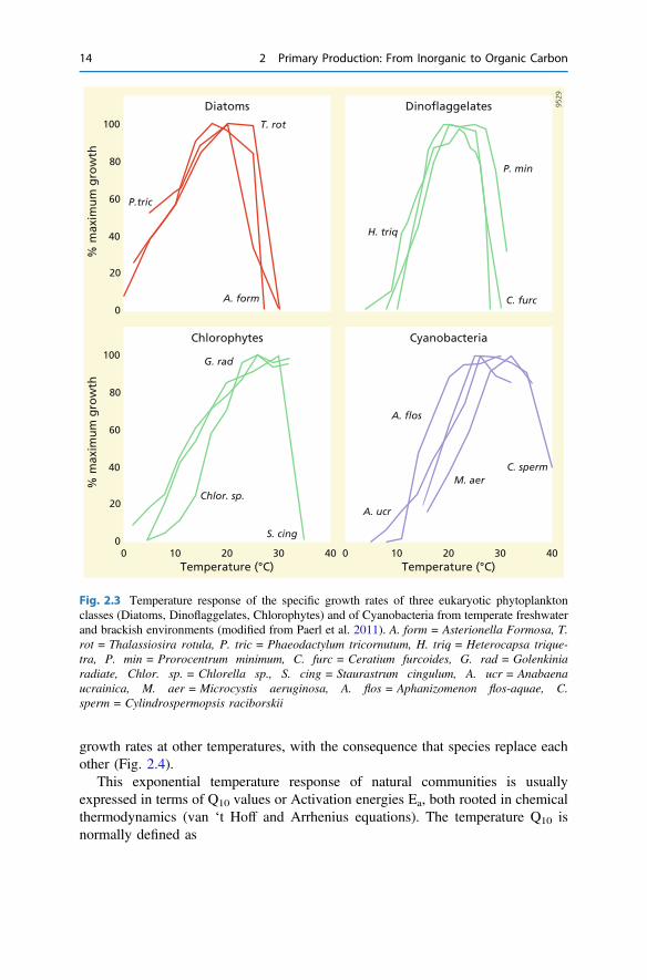
and then typically declines relatively more rapidly: i.e. the response curve is oftenskewed to the left. In other words, phytoplankton growing near its optimum tem-perature is more sensitive to warming than to cooling (Fig. 2.3).

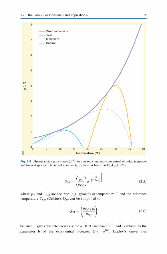
Although populations show distinct unimodal responses to temperature, mixedcommunities, and thus ecosystems, usually exhibit a smooth, monotonical increasebest described by an exponential (l ¼ aebT , Fig. 2.4). The thermal response canthen be described by

l ¼ aebT 1� T � Toptwidth=2

� �2" #

ð2:4Þ

where a and b are empirical parameters describing the maximum envelope for themixed community and Topt and width describe the maximum growth rate andtemperature range of individual populations. Eppley’s (1972) seminal work ontemperature and phytoplankton growth in the sea reported values of 0.59 for a and0.0633 for b. Note that this community response provides an upper limit forindividual species and that high growth rates for individual species trade off with

0

0.2

0.4

0.6

0.8

1

1.2

1.4

1.6

1.8

2

0.2 2 20 2000.02 0.2 2 20 200

µ (

d-1)

Cell size (µm) Cells size (µm)

9529

Cyanobacteria

Chlorophyte

CoccolithophoreDiatom

Dinoflagellate(a) (b)

Fig. 2.2 a The relationship between growth rate and phytoplankton cell size and modelprediction (grey curve) (Ward et al. 2017). b The relationship between growth rate andphytoplankton cell size (solid black line). Maximum nutrient uptake and requirement per cell scalepositively with cell size (dashed blue line), while theoretical maximum growth rates scalenegatively (solid blue line)

2.2 The Basics (For Individuals and Populations) 13

growth rates at other temperatures, with the consequence that species replace eachother (Fig. 2.4).

This exponential temperature response of natural communities is usuallyexpressed in terms of Q10 values or Activation energies Ea, both rooted in chemicalthermodynamics (van ‘t Hoff and Arrhenius equations). The temperature Q10 isnormally defined as

0

20

40

60

80

100

0

20

40

60

80

100

0 10 20 30 40 0 10 20 30 40

% m

axim

um

gro

wth

% m

axim

um

gro

wth

Temperature (°C) Temperature (°C)95

29

Diatoms Dinoflaggelates

Chlorophytes Cyanobacteria

T. rot

H. triq

G. rad

S. cing

Chlor. sp.

A. flos

A. ucr

M. aerC. sperm

P. min

C. furc

P.tric

A. form

Fig. 2.3 Temperature response of the specific growth rates of three eukaryotic phytoplanktonclasses (Diatoms, Dinoflaggelates, Chlorophytes) and of Cyanobacteria from temperate freshwaterand brackish environments (modified from Paerl et al. 2011). A. form = Asterionella Formosa, T.rot = Thalassiosira rotula, P. tric = Phaeodactylum tricornutum, H. triq = Heterocapsa trique-tra, P. min = Prorocentrum minimum, C. furc = Ceratium furcoides, G. rad = Golenkiniaradiate, Chlor. sp. = Chlorella sp., S. cing = Staurastrum cingulum, A. ucr = Anabaenaucrainica, M. aer = Microcystis aeruginosa, A. flos = Aphanizomenon flos-aquae, C.sperm = Cylindrospermopsis raciborskii


Q10 ¼ lTlRef

!e

10

T�TRefð Þ� �

ð2:5Þ

where µT and µRef are the rate (e.g. growth) at temperature T and the referencetemperature TRef (Celsius). Q10 can be simplified to

Q10 ¼lRef þ 10

lRef

!ð2:6Þ

0

1

2

3

4

5

6

7

8

0 5 10 15 20 25 30 35 40

µ (

d-1)

Temperature (°C) 9529

Mixed community

Polar

Temperate

Tropical

Fig. 2.4 Phytoplankton growth rate (d−1) for a mixed community comprised of polar, temperateand tropical species. The mixed community response is based on Eppley (1972)

because it gives the rate increases for a 10 °C increase in T and is related to theparameter b of the exponential increase: Q10 ¼ e10b: Eppley’s curve thus


corresponds to a Q10 of 1.88. Typical Q10 values for biological processes arebetween 2 and 3.

The Arrhenius equation is very similar and reads

l ¼ Ae�EaRT ð2:7Þ

where A is a pre-exponential factor (time−1), Ea is the activation energy (J mol−1),R is the universal gas constant (8.314 J mol−1 K−1) and T is the absolute tem-perature (K). Sometimes the universal gas constant R is replaced by the Boltzmanconstant k (8.617 105 eV K−1) and then Ea is expressed in eV (energy per mole-cule) rather than J mol−1. For the temperature range of seawater, Ea and Q10 valuesare related via

Ea ¼ �RlnQ10

1T � 1

TRef

� � andQ10 ¼ e

EaRð Þ 10

T �TRefð Þ� �

; ð2:8Þ

where T is again given in degrees Kelvin. Eppley’s Q10 of 1.88 corresponds toactivation energies of about 0.47 eV or 45 kJ mol−1 at 20 °C. One should realizethat this is the optimal community temperature response, i.e. no other limitingfactors. Apparent activation energies and Q10 values in the ocean are *0.30 eV(29 kJ mol−1) and *1.5, respectively, close to that of Rubisco (Edwards et al.2016).

2.2.3 Light

Photosynthesis is a light dependent reaction, and light intensity has a major impacton growth rates. The relationship between photosynthesis and irradiance is nor-mally presented as a P versus E curve, where E refers to radiant energy (mol quantam2 s−1). Multiple equations have been presented to represent the photosynthesis tolight relation, which differ in the number of parameters and whether or not theyinclude the photo-inhibition effect at high light intensities or respiration of theautotroph. Photorespiration, the breakdown of photo-labile, intermediate carbonfixation products, is important in full-light exposed organisms, such as terrestrialplants, microphytobenthos and phytoplankton in the surface layer.

Common simple limitation functions are the hyperbolic, Monod model:

flim Eð Þ ¼ E

EþKEð Þ ð2:9Þ

where flim(E) is the light limitation function (0 < flim(E) < 1), KE is alight-saturation parameter (typically 50–150 lmol quanta m−2 s−1 for marinephytoplankton), and the Steele model (1962):


flim Eð Þ ¼ E

Emaxe

1� EEMax

� �ð2:10Þ

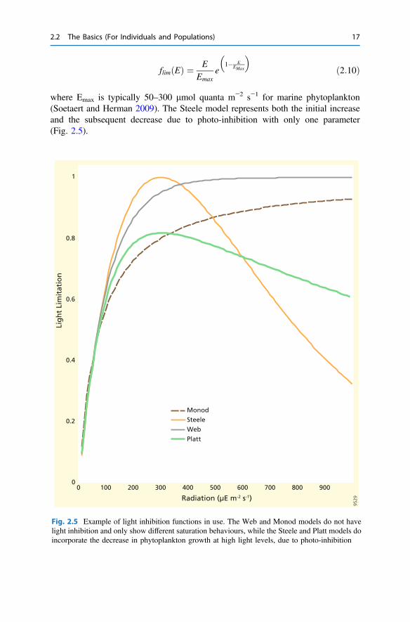
where Emax is typically 50–300 lmol quanta m−2 s−1 for marine phytoplankton(Soetaert and Herman 2009). The Steele model represents both the initial increaseand the subsequent decrease due to photo-inhibition with only one parameter(Fig. 2.5).

0

0.2

0.4

0.6

0.8

1

0 100 200 300 400 500 600 700 800 900

Lig

ht

Lim

itat

ion

Radiation (µE m-2 s-1)

9529

Monod

Steele

Web

Platt

Fig. 2.5 Example of light inhibition functions in use. The Web and Monod models do not havelight inhibition and only show different saturation behaviours, while the Steele and Platt models doincorporate the decrease in phytoplankton growth at high light levels, due to photo-inhibition


The Webb et al. (1974) model is based on an exponential:

flim Eð Þ ¼ 1� 1� eaE

Pmaxð Þh ið2:11Þ

where Pmax is the maximum rate at high light and a is the initial slope (increase in Pwith E at low light intensity). This equation ignores photo-inhibition. Alternatively,one can use the two-parameter Platt et al. (1980) equation:

flim Eð Þ ¼ 1� 1� eaE

Pmaxð Þh ie

�bEPmaxð Þh i

ð2:12Þ

where is b the intensity at the onset of photo-inhibition. Figure 2.5 illustrates thelight limitation functions or PE curves presented above.

2.2.4 Nutrient Limitation

Growing phytoplankton needs a steady supply of resources to maintain growth.Nutrient uptake and growth kinetics are usually described using Monod or Droopkinetics. The former is the simpler model and normally used for steady-stateconditions, while the Droop or internal quota model is preferred for transientconditions, e.g. in fluctuating environments. The equation for nutrient limitationfollowing Monod kinetics is:

l ¼ lmaxS

SþKl� or flim Sð Þ ¼ S

SþKl� ; ð2:13Þ

where S is the substrate concentration of the medium water, flim(S) is the nutrientlimitation function, lmax is the maximal growth rate, and Kl is the half saturationconstant for growth.

The Droop equation expresses growth rate as a function of the cellular quota(Q) of the limiting nutrient (Droop 1970):

l ¼ l0max

Q� Qmin

Qð2:14Þ

where Qmin is the minimum cellular quota for growth. Maximum growth rate onsubstrate (lmax) and cellular quota l

0max

� are related via lmax ¼ l

0max

Qmax�QminQmax

where Qmax is the maximum cellular quota if S increases.


2.3 From Theory and Axenic Mono-Cultures to MixedCommunities in the Field

Progress in theory, creativity in experimental design, and dedicated hard laboratorywork has generated process-based understanding of phytoplankton growth in thelaboratory. This body of knowledge has deepened our understanding and guidedour modelling efforts and field observation strategies, but we need to make manyassumptions before we can apply this mechanistic approach to the field.

Let us return to our master Eq. (2.1): P = µ�B�flim (resources, environmentalconditions). Ignoring environmental conditions, such as temperature, and substi-tuting the simplest expressions introduced above we arrive at:

P ¼ lmax � B � E

EþKEð Þ �S

SþKl� ð2:15Þ

This equation for primary production contains 6 terms that need to be quantified forthe case of a single limiting nutrient and a single phytoplankton species. The lightavailability (E) and nutrient concentration (S) display spatial and temporal gradientsin nature, and the maximum growth rate µmax and half-saturation dependences (KE

and Kl) require experimental or laboratory studies.

2.3.1 Does Diversity Matter or Not?

One of the most critical restrictions on the use of mechanistic complex models isrelated to phytoplankton diversity. Hutchinson (1961) identified the paradox thatphytoplankton is highly diverse, despite the limited range of resources they com-pete for, in direct contrast to the competitive exclusion principle (Hardin 1960).Seawater typically contains tens of different species of primary producers, many forwhich there are no maximum growth data and known limitation functions.Accordingly, it is not feasible to simply apply Eq. 2.15 to individual species in thefield and sum their contributions to obtain the primary production. Besides thesetheoretical arguments against the single species approach, there are also empiricalreasons. Primary production and its dependence on environmental conditions(nutrients, temperature, light) are normally quantified at the community level in theabsence of techniques to quantify species-specific primary production in naturalwaters. This discrepancy between, on the one hand, mechanistic, single-speciesapproaches in the laboratory and, on the other hand, quantification of communityresponses and activities is somewhat unfortunate (Box 2.2).

2.3 From Theory and Axenic Mono-Cultures … 19

2.3.2 Chl the Biomass Proxy

The biomass of the primary producer (B) is the second term in our master equationand quantifying this term in natural systems is more difficult than one initiallywould anticipate. Particulate organic carbon (POC) concentrations (g C per unitvolume) are a direct measure of phytoplankton biomass in laboratory settings withaxenic cultures. However, in natural systems, the pool of particulate organic carboncomprises not only a mixture of phytoplankton species, each with its own maxi-mum growth rate, temperature, light and nutrient dependence, but also a variableand sometimes dominating contribution of detritus (dead organic matter), bacteriaand other heterotrophic organisms. It is for this reason that chlorophyll concen-trations (Chl) are used as a proxy for living primary producer biomass. Therationale is that Chl is only produced by photosynthesizing organisms, degradesreadily after death of the primary producers and can be measured relatively easilyusing a number of methods. Primary producer biomass (B) can then be calculated ifone knows the C:Chl (or Chl:C) ratio of the phytoplankton. However, this ratiodiffers among species and depends on growth conditions, in particular light andnutrient availability (Cloern et al. 1995). Chl:C ratios vary from*0.003 to*0.055(gC gChl−1; Cloern et al. 1995), complicating going from phytoplankton growth toprimary production. The very reason that Chl is such a good proxy for photosyn-thesizing organisms is also the reason why it is not well suited to the task ofpartitioning itself among different phytoplankton species: it is in all primary pro-ducers harvesting light energy. Accessory and minor pigments such as zeaxanthineand fucoxanthine, do, however, have some potential to resolve differences amongphytoplankton groups, but not at the species level.

2.3.3 Light Distribution

The distribution and intensity of photosynthetically active radiation in seawater isgoverned by the intensity at the sea surface (E0) and scattering and absorption oflight, with the result that light attenuates with depth. The decline of light intensity Ewith water depth z can be described by a simple differential equation, expressingthat a constant fraction of radiation is lost:

dE

dz¼ �kPARE ð2:16Þ

where the proportionally constant kPAR is known as the extinction coefficient (m−1).Solving this equation using the radiation at the seawater-air interface (E0) yields thewell-known Lambert–Beer equation:

E ¼ E0e�kPARz ð2:17Þ


The extinction coefficient kPAR includes the absorption of radiation by water (kw),by the pigments from various primary producers (kChl), by coloured dissolvedorganic matter (kDOC), and by suspended particulate material (kspm). The lightextinction coefficient of pure water (kw � 0.015–0.035 m−1) depends on the wavelength of light, with longer wavelength (red) being adsorbed more strongly thanshorter wavelengths (blue); this is the cause of the blue appearance of clear water.The other light extinction components have a different wavelength dependence: theattenuation coefficients of dissolved organic matter (kDOC; “gelbstoffe”) and detritus(kSPM) increase with shorter wave length, while that of phytoplankton (kChl) variesdepending on the species, i.e. the pigment composition of the primary producers(Kirk 1992; Falkowski and Raven 1997).

Oceanographers often divide ocean waters into two classes with respect to lightabsorption: case 1 waters in which phytoplankton (<0.2 mg Chl a m−3) and itsdebris add only to kw, and case 2 waters which have high pigment concentrationand light attenuation because of (terrestrially derived) dissolved organic carbon andsuspended particulate waters. The overall light attenuation (kPAR) in case 1 waterscan be approximated by (Morel 1988):

kPAR ¼ 0:121� Chl0:428 ð2:18Þ

where Chl is in mg Chl a m−3.Other useful empirical relations link light attenuation (kPAR) to the Secchi depth

(zSec, m), the depth at which a white disk disappears visually:

kPAR ¼ q

zSec; ð2:19Þ

where q varies from 1.7 in case 1 waters to 1.4 in case 2 waters (Gattuso et al. 2006)and

kPAR ¼ 0:4þ 1:09zSec

ð2:20Þ

for turbid estuarine waters (Cole and Cloern 1987).Light attenuation coefficients vary from 0.02 m−1 in oligotrophic waters,

0.5 m−1 in coastal waters, and to >2 m−1 in turbid waters Light attenuation bywater and phytoplankton dominate in the open ocean and on the shelf. In othercoastal waters, including estuaries, phytoplankton and suspended particles domi-nate light attenuation, while light attenuation is primarily due to suspended particlesin more turbid systems (Heip et al. 1995).

The light attenuation governs the euphotic zone depth (zeu, m), i.e., the depthwhere radiation is 1% of the incoming:

ln 0:01 ¼ �kPARzEU or zEU ¼ 4:6kPAR

ð2:21Þ

2.3 From Theory and Axenic Mono-Cultures … 21

The euphotic zone is a key depth horizon in aquatic sciences because photosynthesisis largely limited to this zone. Moreover, the bottom of the euphotic zone is often usedas reference for export of organic matter. Euphotic zone depths vary from about200 m in the oligotrophic ocean, to tens of meters in shelf systems, to meters incoastal waters and a few decimetres in turbid and/or eutrophic estuaries (Fig. 2.6).

2.4 Factors Governing Primary Production

Having presented the factors governing phytoplankton production in laboratorystudies and the limitations in applying that knowledge to natural systems, we haveall the ingredients to explore the factors governing the (depth) distribution and rateof primary production in natural ecosystems.

0.01

0.1

1

10

100

1000

10000

100000

0.001 0.01 0.1 1 10 100 1000 10000

Eup

ho

tic

zon

e d

epth

(m

)

SPM (mg/L) or Chl (mg/m3)

9529

Case 1

Water

Chl

Case 2

SPM

Ocean Shelf Turbid estuary

Fig. 2.6 Conceptual figure of euphotic zone depth (solid black line) as a function of suspendedparticulate matter (SPM, mg L−1) and phytoplankton concentrations (Chl, mg m−3). The euphoticzone is more >200 m in the clearest ocean water with very low phytoplankton and light attenuationby water itself dominates. In most of the ocean, phytoplankton dominates light attenuation andeuphotic zone depth scales with phytoplankton concentration. In estuaries and other turbidsystems, dissolved organic matter and in particular suspended particles attenuate light and theeuphotic zone narrows to less than one meter. Coastal systems and eutrophic parts of the ocean arein between. Case 1 and 2 oceanic waters are indicated. Light attenuation due to phytoplankton wasmodelled following Morel (1988; Eq. 2.18), while that due to suspended particles followed Cloern(1987) and euphotic depth was calculated as 4.6/kPAR


2.4.1 Depth Distribution of Primary Production

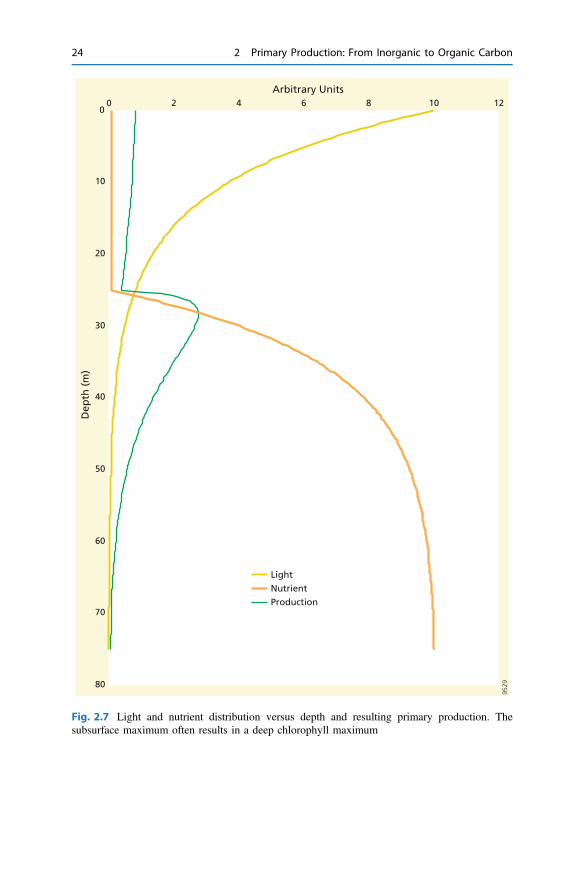
Consider a system with a light profile following the Lambert–Beer equation (2.17)with Eo = 10 mol m−2 d−1 and kPAR = 0.1 m−1 (corresponding to a euphotic zoneof 46 m) and a nutrient pattern as shown in Fig. 2.7. Nutrients are low in the upper25 m (N = 0.1 µmol m−3) and then exponentially increase with a depth coefficient0.1 m−1 to a maximum of 10 µmol m−3.

If we further assume (1) that physical mixing homogenizes phytoplanktonbiomass (B = constant), (2) that there is only one limiting nutrients (N), and (3) thatlight and nutrient limitations can be described by Monod relations with parameterKE and KN. This allows combining µmax and B into a depth independent maximalproduction Pm. The modelled P is then:

P ¼ PmE

EþKEð Þ �N

NþKNð Þ ð2:22Þ

Taking KN and KE values of 1, i.e. 10% of Eo and maximum N at depth, andcombining Eq. 2.22 with the light and nutrient profiles, we can then calculate theprimary production as a function of depth (Fig. 2.7, green curve). Although theselight and nutrient profiles and the model parameters KN and KE numbers have beenchosen arbitrarily, they are reasonable and generate a representative depth profile forprimary production with a subsurface maximum, as observed as a deep chlorophyllmaximum (Fig. 2.8). In the upper 25 m, primary production is rather low because ofnutrient limitation and declines slightly with depth because of light attenuation(Fig. 2.7). Primary production is optimal at depths between 25 and 40 m, i.e. wherethe nutricline and the lower part of the euphotic zone overlap. Primary productionbelow 25 m is primarily light-limited, but accounts for about 75% of thedepth-integrated primary production. Increasing surface-water nutrient concentra-tions or the phytoplankton affinity for nutrients (lowering KN) would increase pri-mary production in the top 25 m, but not so much at depth (Fig. 2.9a). Increasing thephotosynthetic performance at low light levels (lowering KE) would increase pri-mary production at depth (Fig. 2.9b). Phytoplankton living in the surface ocean canthus optimize their performance by investing in nutrient acquisition, while thoseliving in the subsurface would best optimize their light harvesting organs. Thissimple model explains why deep chlorophyll maxima occur in low-nutrient systemsand why the depth distribution of primary production follows light in eutrophicsystems (e.g. during early spring in Bermuda Atlantic station, Fig. 2.8).

2.4.2 Depth-Integrated Production

The overall control of light on depth-integrated production underliessatellite-derived algorithms for primary production and coastal predictive equations.For ecosystem and biogeochemical studies, the focus is on net primary production,i.e. carbon fixation minus phytoplankton respiration, expressed per m2 and unit time

2.4 Factors Governing Primary Production 23

0

10

20

30

40

50

60

70

80

0 2 4 6 8 10 12

Dep

th (

m)

Arbitrary Units

9529

Light

Nutrient

Production

Fig. 2.7 Light and nutrient distribution versus depth and resulting primary production. Thesubsurface maximum often results in a deep chlorophyll maximum


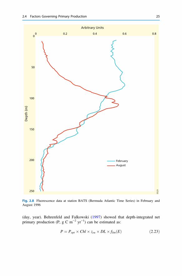
(day, year). Behrenfeld and Falkowski (1997) showed that depth-integrated netprimary production (P, g C m−2 yr−1) can be estimated as:

P ¼ Popt � Chl� zeu � DL� flim Eð Þ ð2:23Þ

50

100

150

200

250

00 0.2 0.4 0.6 0.8

Dep

th (

m)

Arbitrary Units

9529

February

August

Fig. 2.8 Fluorescence data at station BATS (Bermuda Atlantic Time Series) in February andAugust 1996


where Popt is the maximum daily photosynthesis rate (mg C (mg Chl)−1 h−1), zeu isthe euphotic zone depth, DL is day length (h), and flim(E) is a light limitationfunction. The similarity with our master Eq. (2.1) is evident, when nutrient limi-tation and environmental conditions are ignored. Integrating (Eq. 2.1) with depth tozEU, and with time to sunset, we arrive at:

P ¼ Z zEU0

Z sunsetsunrise

lmax � B � flim Eð Þ ð2:24Þ

which is identical to (2.23), with Popt = µmax; Chl = B, RzEU0 ¼ zeu, and

Rsunsetsunrise ¼ DL.Behrenfeld and Falkowski (1997) showed that 85% of the variance in global net

primary production can be attributed to depth integrated biomass (Chl x zeu) and themaximal photosynthesis parameter Popt, with other factors, such as differences inlight limitation functions, depth distributions of phytoplankton biomass and daylength (DL), being less important. Consequently, the most rudimentary modelwould be (Falkowski 1981):

P ¼ w� Chl� zEU � Eo ð2:25Þ

stating that net primary production (P) scales linearly with depth integrated biomass(Chl x zEU), incoming radiation (Eo) and an optimal photosynthetic parameter (w).Similar semi-empirical relations are often used in estuaries (Cole and Cloern 1987;Heip et al. 1995):

P ¼ aþ b Chl� zEU � E0ð Þ ð2:26Þ

10

20

30

40

50

60

70

80

00 1 2 3 4 5 6 7 8 9 0 1 2 3 4 5 6 7 8

Dep

th (

m)

Arbitrary Units Arbitrary Units

9529

Kn = 0.1

K=0.01

Nominal run

Kn =0.5Ke =0.5

Ke=2

Nominal run

Ke =0.1

(a) (b)

Fig. 2.9 a The impact of nutrient availability on the vertical distribution of primary production.Low half-saturation constants KN imply high availability of nutrient for phytoplankton. b Theimpact of light harvesting efficiency on primary production. A high affinity (low KE) for lightcauses higher primary production at depth. The nominal run is presented in Fig. 2.7

where a and b are regression coefficients that are system specific.


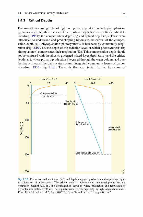
2.4.3 Critical Depths

The overall governing role of light on primary production and phytoplanktondynamics also underlies the use of two critical depth horizons, often credited toSverdrup (1953): the compensation depth (zc) and critical depth (zcr). These wereintroduced to understand and predict spring blooms in the ocean. At the compen-sation depth (zc), phytoplankton photosynthesis is balanced by community respi-ration (Fig. 2.10), i.e. the depth of the radiation level at which photosynthesis (byphytoplankton) compensates their respiration (Ec). This compensation depth shouldnot be confused with the physics governed mixed-layer depth (zmld) and the criticaldepth (zcr), where primary production integrated through the water column and overthe day will equal the daily water column integrated community losses of carbon(Sverdrup 1953; Fig. 2.10). These depths are pivotal to the formation of

0

50

100

150

200

250

0 20 40 0 200 400

mol C m-3 d-1 mol C m-2 d-1

Dep

th (

m)

9529

Critical Depth 200 m

EuphoticDepth 46 m

CompensationDepth 30 m

Integrated production

IntegratedRespiration

Fig. 2.10 Production and respiration (left) and depth integrated production and respiration (right)as a function of water depth. The critical depth is where depth integrated production andrespiration balance (200 m), the compensation depth is where production and respiration ofphytoplankton balance (30 m). The euphotic zone is governed only by light attenuation and is46 m. P0 is 30 mol m−2 d−1; R0 is 0.05*P0; E0 = 30 mol m−2 d−1; kPAR = 0.1 m−1


phytoplankton blooms in the oceans (Sverdrup 1953). If the mixed layer is deeperthan the critical depth (zcr), then phytoplankton will spend relatively too much timeat low irradiances and carbon losses are not compensated by sufficient growth.Conversely, if the mixed layer is shallower than zcr, phytoplankton communitiescan grow and blooms can develop. Assuming that carbon losses (Ro) are constantwith depth, there is no nutrient limitation, and gross primary production is linearlyrelated to radiation, which in turn depends exponentially on depth (Eq. 2.18),primary production is described by:

P ¼ P0e�kPARz, where P0 is the surface productivity. One eventually arrives atfollowing relations for Sverdrup’s critical depth, zcr:

1� ekPARzcr�

kPARzcr¼ EC

E0¼ R0

P0ð2:27Þ

where Ec is the radiation level at the compensation depth and Ro is thedepth-independent community respiration rate (Sverdrup 1953; Siegel et al. 2002).Clearly, light attenuation is a major factor, not only governing zeu, but also zc andzcr. The critical depth (zcr) is usually 4 to 7 times higher than the euphotic zonedepth (zeu). The compensation depth (zc) is typically 50–75% of the euphotic zonedepth (Siegel et al. 2002; Sarmiento and Gruber 2006; Fig. 2.10). For simplicity,the compensation depth is often taken equal to the euphotic zone depth; this shouldbe discouraged, because it implies that community respiration represents only 1%of maximal production. The depth of the euphotic zone (zEU) is an optical depthgoverned by the light attenuation and thus only indirectly impacted by phyto-plankton via their effect on kPAR, while the compensation depth depends on thecommunity structure (algal physiology and heterotrophic community). The Sver-drup critical depth model is simple, instructive and predictive: it can explain bloominitiation when mixed layers shallow and link it to physical sensible and quantifi-able parameters. However, it is sometimes difficult to apply because of inconsis-tencies and uncertainties in the parameterisation (phytoplankton vs. communityrespiration and other phytoplankton losses) and the validity of the assumptions (nonutrient limitation, well-mixed layer).

The critical depth horizon concept has been developed for deep waters, but asimilar approach can be applied to shallow ecosystems. In shallow coastal systems,it is the relative importance of water depth and euphotic zone depth that governs(a) where production occurs and (b) whether phytoplankton biomass will increaseor not. If water depth is less than the euphotic depth (zEU) light reaches the seafloorand primary production by microbial photoautotrophs (microphytobenthos), as wellas macroalgae and seagrasses, may occur. Gattuso et al. (2006) showed that thismay happen over about 1/3 of the global coastal ocean. If water depth exceeds theeuphotic zone by more than a factor 4–7 then phytoplankton losses in the darkcannot be compensated fully by photosynthesis and phytoplankton communitieswill lose biomass (Cloern 1987; Heip et al. 1995). Vice versa, if water depth <4–7times ZEU phytoplankton growth is maintained. Consequently, shallowing ofecosystems (e.g. water flowing over a tidal flat or development of stratification)


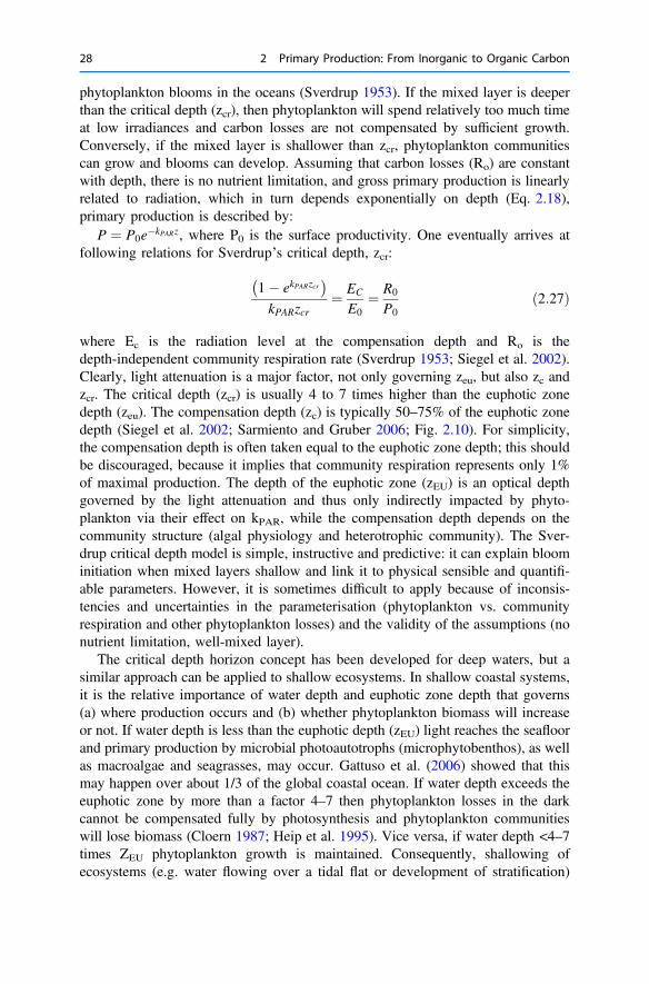
stimulates phytoplankton community growth, all other factors remaining equal,while deepening of water bodies will cause a decline. Moreover, in turbid systemswhere the light attenuation (kPAR), and thus zEU (Fig. 2.7), are governed by sus-pended particulate matter dynamics, phytoplankton communities may experiencevariable twilight conditions and have difficulty maintaining positive growth. Con-sequently, when turbid rivers and estuarine waters with high nutrients reach the sea,particles settle and light climate improves, phytoplankton blooms may develop andutilize the nutrients (Fig. 2.11).

Sverdrup’s critical depth hypothesis is based on the assumption that phyto-plankton biomass and phytoplankton losses are homogenously distributed in themixed layer. However, the mixed layer with uniform temperature as used inSverdrup’s approach does not match with the layer of turbulent mixing in the ocean(Franks 2015). It is more realistic to represent phytoplankton biomass (B) asgoverned by the balance between production, respiration losses and transport byeddy diffusion and particle settling. Again, we assume gross primary production islinearly related to radiation (which declines exponentially); hence: P ¼ P0e�kPARz.Phytoplankton respiration loss is considered a first order process: Loss ¼ rB with afirst-order rate constant (r). Under the assumption of steady-state we then arrive at(see Box 1.1):

Kzd2B

dz2� w

dB

dz� rB ¼ P0e

�kPARz ð2:28Þ

Low LightHigh Nutrient

High LightLow Nutrient

Algea

Fig. 2.11 Conceptualpicture of phytoplanktonbloom in estuarine plume


where Kz is the vertical eddy diffusion coefficient (m2s−1), w is the settling velocity(m s−1; positive downwards), the other terms have been defined before. Consid-ering a semi-infinite domain, i.e. dBdx ¼ 0 at large depth, and phytoplankton biomassB0 at the water-air interface, we obtain the following solution:

B ¼ B0 � P0

Kzk2PAR þwkPAR � r

� �eaz þ P0

Kzk2PAR þwkPAR � re�kPARz ð2:29Þ

with a ¼ w�ffiffiffiffiffiffiffiffiffiffiffiffiffiffiw2 þ 4rKz

p2Kz

:

The second exponential term accounts for light-dependent production, while thefirst exponential comprises water-column mixing, phytoplankton settling, andphytoplankton losses. To simplify matters, we assume that phytoplankton biomassis zero at the air-water interface. The first and second term then balance ifw�

ffiffiffiffiffiffiffiffiffiffiffiffiffiffiw2 þ 4rKz

p2Kz

¼ �kPAR. After re-arrangement to isolate the eddy diffusion coefficient,

we obtain

Kz ¼ r � kPARw

k2PARð2:30Þ

In other words, the vertical eddy diffusion coefficient Kz should be less than r�kPARwk2PAR

for positive values of phytoplankton biomass (B).Huisman et al. (1999) presented a more elaborate model on phytoplankton

growth in a turbulent environment, including a feedback between phytoplanktonbiomass and kPAR. Through scaling and numerical analysis of a model withoutphytoplankton sinking (w = 0), they derived a relationship between the maximumturbulent mixing coefficient Kz and kPAR: Kz ¼ 0:31

k2PAR. If we also ignore phyto-

plankton advection (w = 0 in Eq. 2.30), Kz\ rk2PAR

, fully consistent with Huisman

et al. (1999). The critical turbulence level for phytoplankton growth is thusinversely related to the square of the attenuation of light. Moreover, the phyto-plankton loss is the scaling factor. For turbid systems such as estuaries and othercoastal systems with high light attenuation (kPAR), turbulent mixing should beminimal to allow net growth, consistent with observations by Cloern (1991) thatphytoplankton blooms develop during neap tide when turbulent mixing intensity islowest. Conversely, in clear, oligotrophic waters, light attenuation is limited andphytoplankton blooms can occur at relatively high mixing rates. Sinking phyto-plankton (w > 0) will lower the numerator of Eq. 2.30 and thus lower the criticalturbulence levels, while buoyant phytoplankton (w < 0) will increase the maximalallowable turbulence, and thus the scope for phytoplankton growth.


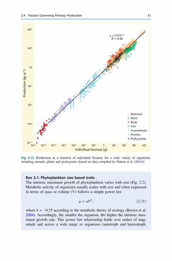
Box 2.1: Phytoplankton size based traitsThe intrinsic maximum growth of phytoplankton varies with size (Fig. 2.2).Metabolic activity of organisms usually scales with size and when expressedin terms of mass or volume (V) follows a simple power law

l ¼ aVb; ð2:31Þ

where b = −0.25 according to the metabolic theory of ecology (Brown et al.2004). Accordingly, the smaller the organism, the higher the intrinsic max-imum growth rate. This power law relationship holds over orders of mag-nitude and across a wide range or organisms (autotroph and heterotroph,

10-11

10-8

10-5

10-2

10

1004

1007

10-14 10-12 10-10 10-8 10-6 10-4 10-2 1 102 104 106 108

Pro

du

ctio

n (

gr

yr-1)

Individual biomass (g)

y = 3.57x0,75

R2 = 0.98

Mammal

Birds

Fish

Invertebrate

Plant

Protists

Prokaryotes

Fig. 2.12 Production as a function of individual biomass for a wide variety of organisms,including animals, plants and prokaryotes (based on data compiled by Hatton et al. (2015))


eukaryotes and prokaryotes; e.g., Fenchel 1973) and implies that smallerorganisms have the highest intrinsic growth (Fig. 2.12).

However, some cell components are non-scaleable, such as the genomeand membrane, and consequently this power-law appears to break down inthe range of nanoplankton (2–20 µm). There is a trade-off between the sizedependence of physiological traits (Ward et al. 2017). Burmaster’s (1979)equation can be used to illustrate this:

lsize ¼lmax � hsize

lmax � Qmin þ hsize; ð2:32Þ

where the maximum growth for a certain size (lsize) depends on maximumnutrient uptake (hsize), minimum cell quota (Qmin) and theoretical maximumgrowth rate (lmax). Maximum nutrient uptake and requirement per cell scalepositively with cell size (Fig. 2.2b, dashed blue line), while theoreticalmaximum growth rates scale negatively (Fig. 2.2b solid blue line). The resultis an optimum in growth rate for phytoplankton in the nanoplankton range(Fig. 2.2b, black line). Very small picoplankton cells have a low intrinsicgrowth rate that will increase with size because more volume is then availablefor catalysing and synthesizing. The intrinsic growth rate of microplanktoncells will decrease with increasing size, as with most organisms, for multiplereasons, including the increase in intracellular transport distances betweencellular machineries (Marañón et al. 2013).

Box 2.2: Phytoplankton diversity, rate measurements and biogeo-chemical modelsThe high number of different species in each water sample poses a challenge tolink the species-specific growth parameters obtained in the laboratory withmeasurements of phytoplankton growth in the field and modelling of phyto-plankton primary production for natural, mixed communities. Gross primaryproduction is normally quantified by the production of oxygen, using either18O-labelling or the differential evolution of oxygen in light and dark. The mostcommon technique for measuring primary production is the 14C labelling tech-nique, but this method provides a result in between gross and net photosynthesis,depending on the duration of the incubation. Both approaches quantify primaryproduction for the total community, rather than for specific species. Biologicaloceanographers have developed methods to quantify group-specific primaryproduction, based on dilution approaches or the incorporation of isotopicallylabelled bicarbonate into biomarker or flow-cytometry separated groups oforganisms (Laws 2013). These group-specific primary productionmeasurementscan be compared more directly to laboratory data.


Biogeochemical modellers have explored a number of strategies toincorporate differences among phytoplankton species into their ecosystemmodels; e.g. the plankton functional group approach and phytoplankton sizeor trait based approaches. The former approach is limited to a few planktongroups that are representative for certain biogeochemical fluxes (e.g. N2-fixers, diatoms, small and large phytoplankton, coccoliths; Sarmiento andGruber 2006). The size-based approach makes use of the systematic rela-tionships between phytoplankton size and activity (e.g. Fig. 2.2), but someprocesses do not scale in a simple way with size. Trait- and genome-basedapproaches are the most recent, and they consider emergent phenomena(Follows et al. 2007). These approaches are instructive and needed to furtherour understanding and predictive capabilities in times of global change, butthey are so far difficult to link with observations in the field.

References

Behrenfeld MJ, Falkowski PG (1997) A consumers’ guide to phytoplankton primary productionmodels. Limnol Oceanogr 42:1479–1491

Brown JH, Gillooly JF, Allen AP, Savage VM, West GB (2004) Toward a metabolic theory ofecology. Ecology 85:1771–1789

Burmaster DE (1979) The continuous culture of phytoplankton: mathematical equivalence amongthree steady-state models. Am Nat 113:123–134

Cloern JE (1987) Turbidity as a control on phytoplankton biomass and productivity in estuaries.Cont Shelf Res 7:1367–1381

Cloern JE (1991) Tidal stirring and phytoplankton bloom dynamics in an estuary. J Mar Res49:203–221

Cloern JE, Grenz C, Vidergar LL (1995) An empirical model of the phytoplankton chlorophyll:-carbon ratio—the conversion factor between productivity and growth rate. Limnol Oceanogr40:1313–1321

Cole BE, Cloern JE (1987) An empirical model for estimating phytoplankton productivity inestuaries. Mar Ecol Prog Ser 36:299–305

Davidson K, Wood G, John EH, Flynn KJ (1999) An investigation of non-steady-state algalgrowth. I. An experimental model ecosystem. J Plankton Res 21:811–837

Droop MR (1970) Vitamin B12 and marine ecology. V. Continuous culture as an approach tonutritional kinetics. Helgoländer Meeresun 20:629–636

Dunne JP, Sarmiento JL, Gnanadesikan A (2007) A synthesis of global particle export from thesurface ocean and cycling through the ocean interior and on the seafloor. Glob BiogeochemCycles, 21:GB4006. https://doi.org/10.1029/2006gb002907

Edwards KF, Thomas MK, Klausmeier CA, Litchman E (2016) Phytoplankton growth and theinteraction of light and temperature: a synthesis at the species and community level. LimnolOceanogr 61:1232–1244

EppleyRW (1972) Temperature and phytoplankton growth in the sea. Fish B.-NOAA70:1063–1085Falkowski PG (1981) Light-shade adaptation and assimilation numbers. J Plankton Res

3(2):203–216Falkowski PG, Raven JA (1997) Aquatic photosynthesis. Blackwell


http://dx.doi.org/10.1029/2006gb002907

Fenchel T (1973) Intrinsic rate of natural increase: the relationship with body size. Oecologia14:317–326

Field CB, Behrenfeld MJ, Randerson JT, Falkowski PG (1998) Primary production of thebiosphere: integrating terrestrial and oceanic components. Science 281:237–240

Follows MJ, Dutkiewicz S, Grant S, Chisholm SW (2007) Emergent biogeography of microbialcommunities in a model ocean. Science 315:1843–1846

Franks PJS (2015) Has Sverdrup’s critical depth hypothesis been tested? Mixed layers vs.turbulent layers. ICES J Mar Sci 72:1897–1907

Gattuso JP, Gentilli B, Duarte C, Kleypass J, Middelburg JJ, Antoine D (2006) Light availabilityin the coastal ocean: impact on the distribution of benthic photosynthetic organism andcontribution to primary production. Biogeosciences 3:489–513

Hardin G (1960) The competitive exclusion principle. Science 131:1292–1297Hatton IA, McCann KS, Fryxell JM, Davies TJ, Smerlak M, Sinclair ARE, Loreau M (2015) The

predator-prey power law: biomass scaling across terrestrial and aquatic biomes. Science, 349:aac6284. https://doi.org/10.1126/science.aac6284

Heip CHR, Goosen NK, Herman PMJ, Kromkamp J, Middelburg JJ, Soetaert K (1995) Productionand consumption of biological particles in temperate tidal estuaries. Oceanogr Mar Biol AnnRev 33:1–150

Huisman J, van Oostveen P, Weissing FJ (1999) Critical depth and critical turbulence: twodifferent mechanisms for the development of phytoplankton blooms. Limnol Oceanogr44:1781–1787

Hutchinson GE (1961) The paradox of the plankton. Am Nat 95:137–145Kirk JTO (1992) The nature and measurement of the light environment in the ocean. In:

Falkowski PG, Woodhead AD, Vivirito K (eds) Primary productivity and biogeochemicalcycles in the sea. Environmental Science Research, vol 43. Springer, Boston

Laws EA (2013) Evaluation of in situ phytoplankton growth rates: a synthesis of data from variedapproaches. Ann Rev Marine Sci 5:247–268

Marañón E, Cermeño P, López-Sandoval DC, Rodríguez-Ramos T, Sobrino C, Huete-Ortega M,Blanco JM, Rodríguez J (2013) Unimodal size scaling of phytoplankton growth and the sizedependence of nutrient uptake and use. Ecol Lett 16:371–379

Middelburg JJ (2011) Chemoautotrophy in the ocean Geoph. Res Lett 38:L24604. https://doi.org/10.1029/2011GL049725

Morel A (1988) Optical modeling of the upper ocean in relation to its biogenous matter content(case I waters). J Geophys Res 93:10749–10768

Paerl HW, Hall NS, Calandrino ES (2011) Controlling harmful cyanobacterial blooms in a worldexperiencing anthropogenic and climatic-induced change. Sci Total Environ 409:1739–1745

Platt TC, Gallegos L, Harrison WG (1980) Photo-inhibition of photosynthesis in naturalassemblages of marine phytoplankton. J Mar Res 38(1980):687–701

Sarmiento J, Gruber N (2006) Ocean biogeochemical dynamics. Princeton University Press, p 526Siegel DA, Doney SC, Yoder JA (2002) The North Atlantic spring phytoplankton bloom and

Sverdrup’s critical depth hypothesis. Science 296:730–733Smith SV (1981) Marine macrophytes as a global carbon sink. Science 211:838–840Steele JH (1962) Environmental control of photosynthesis in the sea. Limnol Oceanogr 7:137–150Soetaert K, Herman PMJ (2009) A practical guide to ecological modelling. Springer, p 372Sverdrup HU (1953) On conditions for the vernal blooming of phytoplankton. Journal du Conseil

International pour l’Exploration de la Mer 18:287–295WardBA,Marañón E, SautereyB, Rault J, ClaessenD (2017) The size dependence of phytoplankton

growth rates: a trade-off between nutrient uptake and metabolism. Am Nat 189:170–177Webb WL, Newton M, Starr D (1974) Carbon dioxide exchange of Alnus rubra: a mathemical

model. Oecologia 17:281–291


http://dx.doi.org/10.1126/science.aac6284

http://dx.doi.org/10.1029/2011GL049725

http://dx.doi.org/10.1029/2011GL049725



References 35


3The Return from Organic to InorganicCarbon

Almost all the organic matter produced is eventually consumed and respired toinorganic carbon because organic matter preservation via burial in accumulatingsediments (*0.2–0.4 Pg y−1) represents only a very small fraction of that produced.Global phytoplankton production is about *50 Pg C y−1, while phytoplanktonbiomass is *1 Pg, implying a turnover of one week (0.02 y−1). Marine macro-phytes have a similar global biomass, but a production of only 1 Pg C y−1; theturnover is thus *1 y−1 (Smith 1981). These high turnover rates (compared withglobal terrestrial vegetation turnover of about one to two decades, Field et al. 1998)imply not only steady production, but also efficient consumption of organic matter.There are multiple organic matter loss pathways (respiration by autotrophs andheterotrophs, grazing, viral lysis, detrital route), but all eventually result in respi-ration and release of inorganic carbon.

Biogeochemists constructing carbon budgets normally lump together the variousorganic matter loss pathways and focus instead on the quantification of the organiccarbon to inorganic carbon transformation. However, for a more detailed under-standing, the elucidation of the link with other biogeochemical cycles and theidentity of organisms involved, the various pathways have to be resolved. Beforediscussing the processes and mechanisms involved in these routes, it is instructiveto distinguish between living organic matter that has the capability to reproduce(primary and secondary producers) and dead organic matter (i.e. detritus). Whileliving organic matter is, by definition, fresh and thus labile, detrital organic matterpools represent a heterogeneous mixture of compounds from various sources whichhave been mixed together and which may have distinct compositions, degradationhistories and reactivities (Box 3.1). Another distinction is between organic matter inthe dissolved and particulate phases. Concentrations of DOC (order 10–100 mmol m−3) are usually one order of magnitude higher than those of POC(order 1–10 mmol m−3) in the euphotic zone of the ocean, while sediment POC(order 106 mmol m−3) concentrations are normally three orders of magnitude higherthan those of DOC in pore water (100–1000 mmol m−3). Moreover, the DOC poolis detrital (with viruses), while the particulate organic carbon pool usually


37




https://doi.org/10.1007/978-3-030-10822-9_3

represents a mixture of living organisms, their remains, and other detrital organiccarbon inputs. As we discussed in Chap. 2, the POC concentrations in the watercolumn can be a poor proxy for phytoplankton carbon. This distinction betweendissolved and particulate pools is pivotal for understanding the fate of organicmatter. Dissolved organic matter is transported as a solute with the water, whileparticulate organic matter is subject to gravity, which results in settling of organicparticles. Consequently, the residence time of DOC in an aquatic system is muchlonger than that of POC. Consumption of dissolved organic matter primarilyinvolves microbes and other small organisms, which use it for energy and nutrientacquisition, while larger organisms generally prefer particulate organic matter.Microbes use extracellular enzymes to solubilize particulate organic matter beforethey can utilize it.

In this chapter, we discuss carbon consumption in the context of the “biologicalpump”. The latter depends on the fraction of primary produced organic matter thatsurvives degradation in the euphotic zone and that is exported from surface water tothe ocean interior, where it mineralized to inorganic carbon, with the result thatcarbon is transported against the gradient of dissolved inorganic carbon from thesurface to the deep ocean. This transfer occurs through physical mixing andtransport of dissolved and particulate organic carbon, vertical migrations oforganisms (zooplankton, fish) and through gravitational settling of particulateorganic carbon (Volk and Hoffert 1985; Sarmiento and Gruber 2006). We firstdiscuss carbon consumption pathways in the euphotic zone, then the factors gov-erning export of organic carbon from the euphotic zone and particle degradation inthe ocean interior. Processes specifically related to organic carbon consumption inthe coastal zone are presented in Box 3.2.

3.1 Carbon Consumption Pathway in the Euphotic Zone

For pelagic ecosystems, Legendre and Rassoulzadagan (1995) proposed a contin-uum of trophic pathways with the herbivorous food-chain and microbial loop asfood-web end members (Fig. 3.1). The classical linear food-chain end-memberinvolves grazing by zooplankton on larger phytoplankton and subsequent predationon zooplankton by either larger zooplankton or another predator. In such a linearfood-chain a predator can either lead to high phytoplankton biomass (in a systemwith phytoplankton, herbivore and a predator) or reduced phytoplankton biomass(in a system with four levels). Changes in predator abundance can, thus, lead totrophic cascades (Pace et al. 1999). The microbial loop end-member involves notonly phytoplankton, as basal resource, but also dissolved organic carbon (Azamet al. 1983). Dissolved organic carbon is used by heterotrophic bacteria for growthand respiration, and these heterotrophic bacteria are, in turn, consumed by micro-zooplankton (20–200 lm; ciliates, radiolarian, foraminifera) that are predated uponby larger zooplankton. Consequently, dissolved organic carbon is transformed, viaa bacterial-microzooplankton loop, to zooplankton. These two end-member carbon

38 3 The Return from Organic to Inorganic Carbon

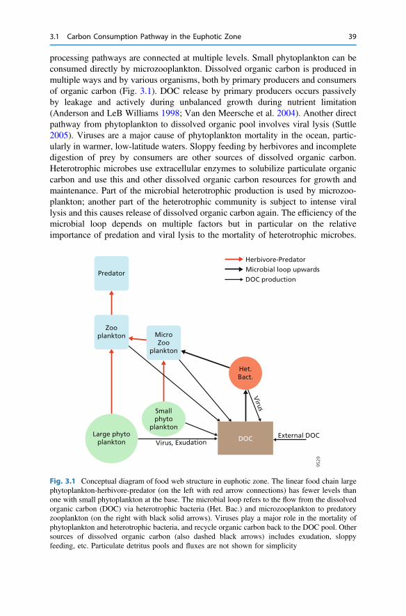
processing pathways are connected at multiple levels. Small phytoplankton can beconsumed directly by microzooplankton. Dissolved organic carbon is produced inmultiple ways and by various organisms, both by primary producers and consumersof organic carbon (Fig. 3.1). DOC release by primary producers occurs passivelyby leakage and actively during unbalanced growth during nutrient limitation(Anderson and LeB Williams 1998; Van den Meersche et al. 2004). Another directpathway from phytoplankton to dissolved organic pool involves viral lysis (Suttle2005). Viruses are a major cause of phytoplankton mortality in the ocean, partic-ularly in warmer, low-latitude waters. Sloppy feeding by herbivores and incompletedigestion of prey by consumers are other sources of dissolved organic carbon.Heterotrophic microbes use extracellular enzymes to solubilize particulate organiccarbon and use this and other dissolved organic carbon resources for growth andmaintenance. Part of the microbial heterotrophic production is used by microzoo-plankton; another part of the heterotrophic community is subject to intense virallysis and this causes release of dissolved organic carbon again. The efficiency of themicrobial loop depends on multiple factors but in particular on the relativeimportance of predation and viral lysis to the mortality of heterotrophic microbes.

9529

Large phytoplankton

Zooplankton

Predator

Smallphyto

plankton

MicroZoo

plankton

Het.Bact.

DOC

Virus

Virus, ExudationExternal DOC

Herbivore-Predator

Microbial loop upwards

DOC production

Fig. 3.1 Conceptual diagram of food web structure in euphotic zone. The linear food chain largephytoplankton-herbivore-predator (on the left with red arrow connections) has fewer levels thanone with small phytoplankton at the base. The microbial loop refers to the flow from the dissolvedorganic carbon (DOC) via heterotrophic bacteria (Het. Bac.) and microzooplankton to predatoryzooplankton (on the right with black solid arrows). Viruses play a major role in the mortality ofphytoplankton and heterotrophic bacteria, and recycle organic carbon back to the DOC pool. Othersources of dissolved organic carbon (also dashed black arrows) includes exudation, sloppyfeeding, etc. Particulate detritus pools and fluxes are not shown for simplicity

3.1 Carbon Consumption Pathway in the Euphotic Zone 39

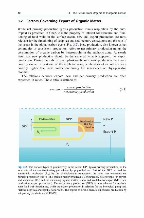
3.2 Factors Governing Export of Organic Matter

While net primary production (gross production minus respiration by the auto-trophs) as presented in Chap. 2 is the property of interest for structure and func-tioning of food webs in the surface ocean, new and export production are mostrelevant for the functioning of deep-sea and sedimentary ecosystems and the role ofthe ocean in the global carbon cycle (Fig. 3.2). New production, also known as netcommunity or ecosystem production, refers to net primary production minus theconsumption of organic carbon by heterotrophs in the euphotic zone. At steadystate, this new production should be the same as what is exported, i.e. exportproduction. During periods of phytoplankton blooms new production may tem-porarily exceed export out of the euphotic zone, while rates of export are tem-porarily higher than new production during the senescence of phytoplanktonblooms.

The relations between export, new and net primary production are oftenexpressed in ratios. The e-ratio is defined as:

e�ratio ¼ export production

net primary productionð3:1Þ

9529

Phytoplankton

RA

ZooplanktonHet. Bac.Detritus

NPP New P

=

Export P

GPP

RH

Fig. 3.2 The various types of productivity in the ocean. GPP (gross primary production) is thetotal rate of carbon fixation/oxygen release by phytoplankton. Part of the GPP is used forautotrophic respiration (RA) by the phytoplankton community, the other part represents netprimary production (NPP). The organic matter produced is consumed by heterotrophs for growthand respiration (RH) and the remaining organic matter is new and available for export (NEP, newproduction, export production). The net primary production (NPP) is most relevant for euphoticzone food web functioning, while the export production is relevant for the biological pump andfuelling deep-sea and benthic food webs. The export or e-ratio divides export/new production bynet primary production (NEP/NPP)


where export production is often quantified via the use of sediment traps (Suess1980). Note that e-ratios based on sediment trap might be biased if dissolvedorganic matter is transported downwards by advection and/or eddy-diffusion and ifzooplankton and other mobile vertical migrating organism contribute significantlyto the total downward flux of organic carbon. An alternative method to quantify therelative importance of new to total production is the f-ratio, based on nitrogen useand recycling:

f�ratio ¼ new production

new productionþ recycled productionð3:2Þ

where new production is assumed to equal nitrate uptake and recycled production istaken equal to ammonium uptake as determined from 15N tracer experiments(Dugdale and Goering 1967). The rationale is that nitrogen availability limits pri-mary production, that nitrate is supplied to the euphotic zone from deeper waters(thus new to euphotic zone) and that recycling of organic nitrogen within theeuphotic zone generates ammonium. Export of organic nitrogen should eventually,on the global scale, be equivalent to nitrate supply from the deep to surface ocean.However, nitrification (ammonium oxidation to nitrite and nitrate) in the euphoticzone, atmospheric deposition, nitrogen fixation and other nitrogen cycling pro-cesses (bacterial uptake of dissolved inorganic nitrogen, dissolved organic nitrogengeneration and use) complicate this simple depiction. At steady state e and f-ratiosshould be the same if the underlying assumptions are correct.

These export ratios vary from *0.04 to *0.72. Although multiple factorscontribute to this range in export ratios (phytoplankton size, community structure,e.g. see Fig. 3.1), temperature and total primary production together account for87% of the variance in export production and ratios (Laws et al. 2000, 2011; Dunneet al. 2005). The empirical model of Laws et al. (2011):

e�ratio ¼ 0:04756 0:78� 0:43T30

� �P0:307 ð3:3Þ

shows that e-ratios depend negatively on temperature (T, in Celsius) and scale withthe power *0.3 to net primary production (P). Export production consequentlyscales to net primary production with a power of *1.3. Temperature is the singlemost important factor (Fig. 3.3), because organic carbon consumption by hetero-trophs is more temperature sensitive than light and nutrient-limited primary pro-duction by phytoplankton (Laws et al. 2000). The impact of primary production onthe export ratio can be explained by the increase in the size (and thus settling rate)of phytoplankton with increasing primary production (Dunne et al. 2005). Theglobal average export ratio is *0.2 with eutrophic, high-latitude systems havinghigh e-ratios and oligotrophic, low-latitude systems having the lowest ratios.

3.2 Factors Governing Export of Organic Matter 41

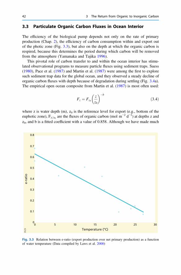
3.3 Particulate Organic Carbon Fluxes in Ocean Interior

The efficiency of the biological pump depends not only on the rate of primaryproduction (Chap. 2), the efficiency of carbon consumption within and export outof the photic zone (Fig. 3.3), but also on the depth at which the organic carbon isrespired, because this determines the period during which carbon will be removedfrom the atmosphere (Yamanaka and Tajika 1996).

This pivotal role of carbon transfer to and within the ocean interior has stimu-lated observational programs to measure particle fluxes using sediment traps. Suess(1980), Pace et al. (1987) and Martin et al. (1987) were among the first to exploresuch sediment trap data for the global ocean, and they observed a steady decline oforganic carbon fluxes with depth because of degradation during settling (Fig. 3.4a).The empirical open ocean composite from Martin et al. (1987) is most often used:

Fz ¼ Fz0z

z0

� ��b

ð3:4Þ

where z is water depth (m), z0 is the reference level for export (e.g., bottom of theeuphotic zone), Fz=z0 are the fluxes of organic carbon (mol m−2 d−1) at depths z andz0, and b is a fitted coefficient with a value of 0.858. Although we have made much

0

0.1

0.2

0.3

0.4

0.5

0.6

0.7

0.8

0 5 10 15 20 25 30

e-ra

tio

Temperature (°C)

9529

Fig. 3.3 Relation between e-ratio (export production over net primary production) as a functionof water temperature (Data compiled by Laws et al. 2000)


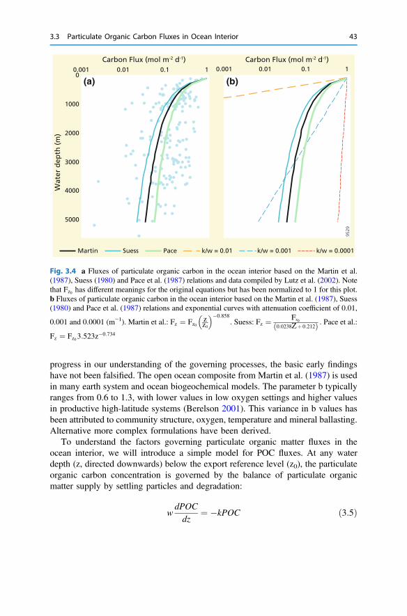
progress in our understanding of the governing processes, the basic early findingshave not been falsified. The open ocean composite from Martin et al. (1987) is usedin many earth system and ocean biogeochemical models. The parameter b typicallyranges from 0.6 to 1.3, with lower values in low oxygen settings and higher valuesin productive high-latitude systems (Berelson 2001). This variance in b values hasbeen attributed to community structure, oxygen, temperature and mineral ballasting.Alternative more complex formulations have been derived.

To understand the factors governing particulate organic matter fluxes in theocean interior, we will introduce a simple model for POC fluxes. At any waterdepth (z, directed downwards) below the export reference level (z0), the particulateorganic carbon concentration is governed by the balance of particulate organicmatter supply by settling particles and degradation:

wdPOC

dz¼ �kPOC ð3:5Þ

0

1000

2000

3000

4000

5000

0.001 0.01 0.1 1 0.001 0.01 0.1 1Carbon Flux (mol m-2 d-1) Carbon Flux (mol m-2 d-1)

Wat

er d

epth

(m

)

9529

Martin Suess Pace k/w = 0.0001k/w = 0.001k/w = 0.01

(a) (b)

Fig. 3.4 a Fluxes of particulate organic carbon in the ocean interior based on the Martin et al.(1987), Suess (1980) and Pace et al. (1987) relations and data compiled by Lutz et al. (2002). Notethat Fz0 has different meanings for the original equations but has been normalized to 1 for this plot.b Fluxes of particulate organic carbon in the ocean interior based on the Martin et al. (1987), Suess(1980) and Pace et al. (1987) relations and exponential curves with attenuation coefficient of 0.01,

0.001 and 0.0001 (m−1). Martin et al.: Fz ¼ Fz0zz0

� ��0:858: Suess: Fz ¼ Fz0

0:0238Zþ 0:212ð Þ : Pace et al.:Fz ¼ Fz0 3:523z

�0:734

3.3 Particulate Organic Carbon Fluxes in Ocean Interior 43

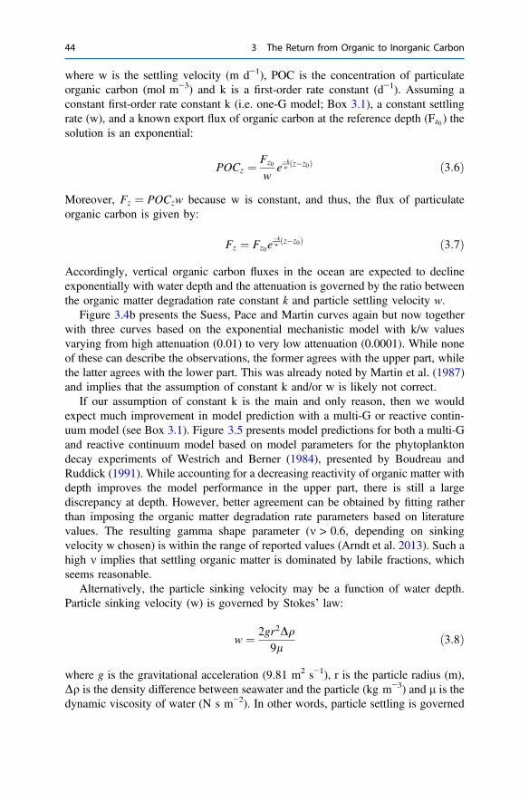
where w is the settling velocity (m d−1), POC is the concentration of particulateorganic carbon (mol m−3) and k is a first-order rate constant (d−1). Assuming aconstant first-order rate constant k (i.e. one-G model; Box 3.1), a constant settlingrate (w), and a known export flux of organic carbon at the reference depth (Fz0 ) thesolution is an exponential:

POCz ¼ Fz0

we�kw z�z0ð Þ ð3:6Þ

Moreover, Fz ¼ POCzw because w is constant, and thus, the flux of particulateorganic carbon is given by:

Fz ¼ Fz0e�kw z�z0ð Þ ð3:7Þ

Accordingly, vertical organic carbon fluxes in the ocean are expected to declineexponentially with water depth and the attenuation is governed by the ratio betweenthe organic matter degradation rate constant k and particle settling velocity w.

Figure 3.4b presents the Suess, Pace and Martin curves again but now togetherwith three curves based on the exponential mechanistic model with k/w valuesvarying from high attenuation (0.01) to very low attenuation (0.0001). While noneof these can describe the observations, the former agrees with the upper part, whilethe latter agrees with the lower part. This was already noted by Martin et al. (1987)and implies that the assumption of constant k and/or w is likely not correct.

If our assumption of constant k is the main and only reason, then we wouldexpect much improvement in model prediction with a multi-G or reactive contin-uum model (see Box 3.1). Figure 3.5 presents model predictions for both a multi-Gand reactive continuum model based on model parameters for the phytoplanktondecay experiments of Westrich and Berner (1984), presented by Boudreau andRuddick (1991). While accounting for a decreasing reactivity of organic matter withdepth improves the model performance in the upper part, there is still a largediscrepancy at depth. However, better agreement can be obtained by fitting ratherthan imposing the organic matter degradation rate parameters based on literaturevalues. The resulting gamma shape parameter (m > 0.6, depending on sinkingvelocity w chosen) is within the range of reported values (Arndt et al. 2013). Such ahigh m implies that settling organic matter is dominated by labile fractions, whichseems reasonable.

Alternatively, the particle sinking velocity may be a function of water depth.Particle sinking velocity (w) is governed by Stokes’ law:

w ¼ 2gr2Dq9l

ð3:8Þ

where g is the gravitational acceleration (9.81 m2 s−1), r is the particle radius (m),Dq is the density difference between seawater and the particle (kg m−3) and l is thedynamic viscosity of water (N s m−2). In other words, particle settling is governed


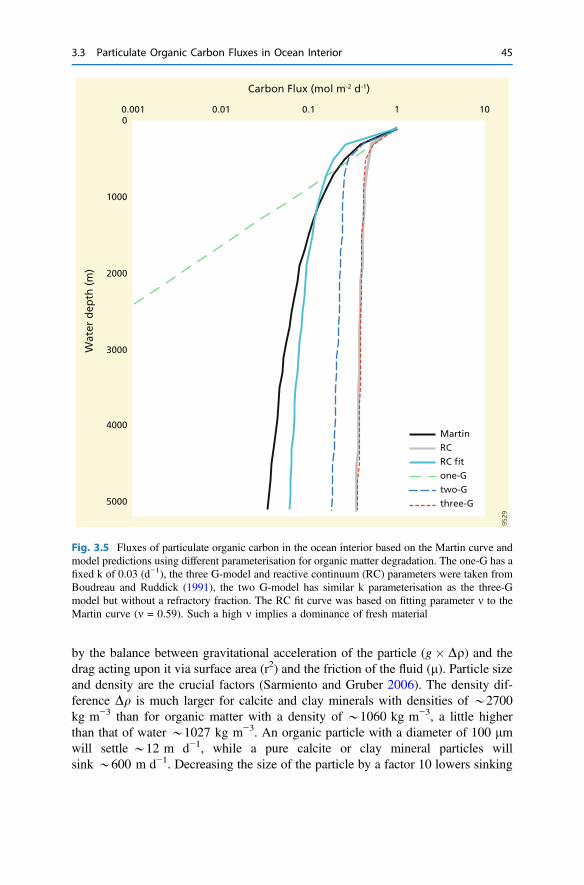
by the balance between gravitational acceleration of the particle (g� Dq) and thedrag acting upon it via surface area (r2) and the friction of the fluid (l). Particle sizeand density are the crucial factors (Sarmiento and Gruber 2006). The density dif-ference Dq is much larger for calcite and clay minerals with densities of *2700kg m−3 than for organic matter with a density of *1060 kg m−3, a little higherthan that of water *1027 kg m−3. An organic particle with a diameter of 100 lmwill settle *12 m d−1, while a pure calcite or clay mineral particles willsink *600 m d−1. Decreasing the size of the particle by a factor 10 lowers sinking

0

1000

2000

3000

4000

5000

0.001 0.01 0.1 1 10

Wat

er d

epth

(m

) Carbon Flux (mol m-2 d-1)

9529

Martin

one-G

three-G

two-G

RC

RC fit

Fig. 3.5 Fluxes of particulate organic carbon in the ocean interior based on the Martin curve andmodel predictions using different parameterisation for organic matter degradation. The one-G has afixed k of 0.03 (d−1), the three G-model and reactive continuum (RC) parameters were taken fromBoudreau and Ruddick (1991), the two G-model has similar k parameterisation as the three-Gmodel but without a refractory fraction. The RC fit curve was based on fitting parameter m to theMartin curve (m = 0.59). Such a high m implies a dominance of fresh material


velocities by a factor 100, because of the r2 dependence, indicating that smallreactive organic particles will never reach the seafloor.

Although Stokes’ law is based on physical principles and generally valid,application to particles in the ocean is not straightforward. Particles are diverse andmade up of aggregates of various plankton types, their detritus, faecal pellets anddifferent mineral phases with distinct densities. Stokes’ law as formulated above isfor spherical particles and most marine particles, organism and their remains maydeviate strongly from this shape, with the consequence that they are somewhat lessdependent on size. Moreover, particles sizes in the ocean vary over orders ofmagnitude. Size spectra analysis show that most mass occurs in the smaller sizeclasses and cannot directly be linked to that of primary producers size spectra.During settling, particles interact, disaggregate and coagulate, with the consequencethat the number and size distribution of particles changes. Natural organic matteraggregates have high porosity, which decreases the density difference betweenwater and particles and thus gravitational acceleration. Nevertheless, settlingvelocities of natural particles have shown to follow a power law with particle size(Clegg and Whitfield 1990; Sarmiento and Gruber 2006). In situ settling velocitieshave been quantified by high-resolution underwater video systems and inferredfrom the time-lag of pulse arrival between sediment traps at different water depth inthe same area. The latter approach showed that particle settling velocities increasedwith depth (Berelson 2002).

To explore the impact of increasing settling velocities a linear and exponentialincrease of particle sinking rates with water depth was assumed (Fig. 3.6b) andEq. 3.5 solved for these situations (Fig. 3.6a). A linear increasing rate of particlesettling from 10 m d−1 at the bottom of the euphotic zone to about 185 m, com-bined with a first-order degradation rate constant (k = 0.03 d−1; *11 y−1) agreeswith the parameterisation of Suess (1980) and Martin et al. (1987). Evidently theinitial assumption of constant first-order rate constants and sinking velocities mightbe questionable.

These agreements between the Martin’s ocean composite model and the reactivecontinuum (with high m) and linear increasing settling rates are not unexpected: it isin the equations. The flux equation for the reactive continuum model with uniformw:

Fz ¼ F0aw

awþ z

� �m

ð3:9Þ

approaches the Martin et al. curve if aw << z. Similarly, the flux equation forconstant reactivity but with linear increasing velocity according to wz = c z (c ind−1) is:

Fz ¼ F0z

z0

� ��kc

ð3:10Þ


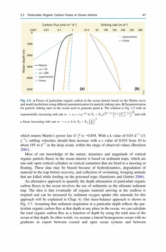
which returns Martin’s power law if �kc is −0.858. With a k value of 0.03 d−1 (11

y−1), settling velocities should then increase with a c value of 0.035 from 10 toabout 185 m d−1 in the deep ocean, within the range of observed values (Berelson2001).

Most of our knowledge of the nature, dynamics and magnitude of verticalorganic particle fluxes in the ocean interior is based on sediment traps, which areone-side open vertical cylinders or conical containers that are fixed to a mooring orfloating. These data may be biased because of hydrodynamics, degradation ofmaterial in the trap before recovery, and collection of swimming, foraging animalsthat are killed while feeding on the poisoned traps (Sarmiento and Gruber 2006).

An alternative approach to quantify the depth attenuation of particulate organiccarbon fluxes in the ocean involves the use of sediments as the ultimate sedimenttrap. The idea is that eventually all organic material arriving at the seafloor isrespired and can be measured by sediment oxygen uptake (the rationale for thisapproach will be explained in Chap. 4). Our mass-balance approach is shown inFig. 3.7. Assuming that sediment respiration at a particular depth reflects the par-ticulate organic carbon flux at that depth at any place in the ocean, we can calculatethe total organic carbon flux as a function of depth by using the total area of theocean at that depth. In other words, we assume a lateral homogenous ocean with nogradients in export between coastal and open ocean systems and between

0

1000

2000

3000

4000

5000

0.001 0.01 0.1 1 10 0 50 100 150 200 250 300

Wat

er d

epth

(m

) Carbon Flux (mol m-2 d-1) Sinking rate (m d-1)

9529

Martin

w = 10

w = 200

exponential

linear

exponential

linear

(a) (b)

Fig. 3.6 a Fluxes of particulate organic carbon in the ocean interior based on the Martin curveand model predictions using different parameterisation for particle sinking rates. b Parameterisationfor particle sinking rates in the ocean used to generate panel a. The solution to Eq. 3.5 with an

exponentially increasing sink rate w ¼ v0 þ v1e�bz is: Fz ¼ Fz0 e�km0

z�z0ð Þ m0 þ m1e�b z�z0ð Þm0 þ m1

� ��km0band with

a linear increasing sink rate w ¼ c z, it is: Fz ¼ Fz0zz0

� ��kc


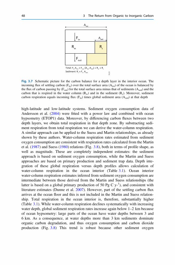
high-latitude and low-latitude systems. Sediment oxygen consumption data ofAndersson et al. (2004) were fitted with a power law and combined with oceanhypsometry (ETOP1) data. Moreover, by differencing carbon fluxes between twodepth layers, we obtain total respiration in that depth zone. By substracting sedi-ment respiration from total respiration we can derive the water-column respiration.A similar approach can be applied to the Suess and Martin relationships, as alreadyshown by these authors. Water-column respiration rates estimated from sedimentoxygen consumption are consistent with respiration rates calculated from the Martinet al. (1987) and Suess (1980) relations (Fig. 3.8), both in terms of profile shape, aswell as magnitude. These are completely independent estimates: the sedimentapproach is based on sediment oxygen consumption, while the Martin and Suessapproaches are based on primary production and sediment trap data. Depth inte-gration of these global respiration versus depth profiles allows calculation ofwater-column respiration in the ocean interior (Table 3.1). Ocean interiorwater-column respiration estimates inferred from sediment oxygen consumption areintermediate between those derived from the Martin and Suess relationships (thelatter is based on a global primary production of 50 Pg C y-1), and consistent withliterature estimates (Dunne et al. 2007). However, part of the settling carbon fluxarrives at the ocean floor and this is not included in the Martin and Suess relation-ship. Total respiration in the ocean interior is, therefore, substantially higher(Table 3.1). While water-column respiration declines systematically with increasingwater depth, global sediment respiration rates increase again below 1–2 km becauseof ocean hypsometry: large parts of the ocean have water depths between 3 and6 km. As a consequence, at water depths more than 3 km sediments dominateorganic carbon degradation, and thus oxygen consumption and carbon dioxideproduction (Fig. 3.8) This trend is robust because other sediment oxygen

9529

AsedFin

Fout

Rw Rs

Atot

Total: Fin Atot = Fout (Atot-Ased) + Rw + Rs

Sediment: Rs = Fin Ased

Fig. 3.7 Schematic picture for the carbon balance for a depth layer in the interior ocean. Theincoming flux of settling carbon (Fin) over the total surface area (Atot) of the ocean is balanced bythe flux of carbon passing by (Fout) for the total surface area minus that of sediments (Ased) and thecarbon that is respired in the water column (Rw) and in the sediment (Rs). Moreover, sedimentcarbon respiration equals incoming flux (Fin) times global sediment area (Ased) at that depth


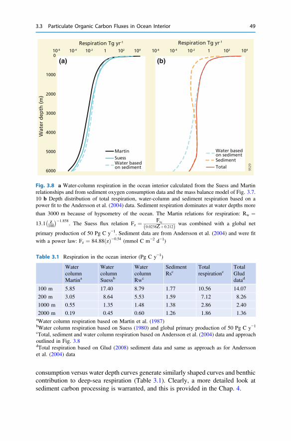
consumption versus water depth curves generate similarly shaped curves and benthiccontribution to deep-sea respiration (Table 3.1). Clearly, a more detailed look atsediment carbon processing is warranted, and this is provided in the Chap. 4.

0

1000

2000

3000

4000

5000

6000

10-6 10-4 10-2 1 102 104 10-6 10-4 10-2 1 102 104

Wat

er d

epth

(m

)Respiration Tg yr-1 Respiration Tg yr-1

9529

Water basedon sediment

SuessMartin Water based

on sediment

Total

Sediment

(a) (b)

Fig. 3.8 a Water-column respiration in the ocean interior calculated from the Suess and Martinrelationships and from sediment oxygen consumption data and the mass balance model of Fig. 3.7.10 b Depth distribution of total respiration, water-column and sediment respiration based on apower fit to the Andersson et al. (2004) data. Sediment respiration dominates at water depths more

than 3000 m because of hypsometry of the ocean. The Martin relations for respiration: Rw ¼13:1 z

100

� ��1:858: The Suess flux relation Fz ¼ Fz0

0:0238Zþ 0:212ð Þ was combined with a global net

primary production of 50 Pg C y−1. Sediment data are from Andersson et al. (2004) and were fitwith a power law: Fz ¼ 84:88 zð Þ�0:54 (mmol C m−2 d−1)

Table 3.1 Respiration in the ocean interior (Pg C y−1)

WatercolumnMartina

WatercolumnSuessb

WatercolumnRwc

SedimentRsc

Totalrespirationc

TotalGluddatad

100 m 5.85 17.40 8.79 1.77 10.56 14.07

200 m 3.05 8.64 5.53 1.59 7.12 8.26

1000 m 0.55 1.35 1.48 1.38 2.86 2.40

2000 m 0.19 0.45 0.60 1.26 1.86 1.36aWater column respiration based on Martin et al. (1987)bWater column respiration based on Suess (1980) and global primary production of 50 Pg C y−1cTotal, sediment and water column respiration based on Andersson et al. (2004) data and approachoutlined in Fig. 3.8dTotal respiration based on Glud (2008) sediment data and same as approach as for Anderssonet al. (2004) data


Box 3.1: Organic matter reactivityDetrital organic matter represents a very heterogeneous pool of thousands oforganic compounds. Individual compounds may originate from variousorganisms, come from different environments, may have been producedrecently or thousands of years ago, and have experienced a different historybefore eventually making up the compound pool of dissolved or particulateorganic matter. Moreover, for particulate organic matter these compoundsmay be associated with different mineral phases or incorporated in variousways into minerals (Arndt et al. 2013). All these factors and intrinsic dif-ferences in reactivity among organic compounds result in large differences inorganic matter reactivity (Middelburg 1989). Organic matter reactivity isusually expressed in terms of a first-order rate constant (k), which originatesfrom the one-G model of marine organic matter degradation (Berner 1964):

dGm

dt¼ �kGm; ð3:11Þ

where Gm is the concentration of metabolizable organic matter, t is time and kis a first-order rate constant (time−1) assumed to be constant in time. Thisequation implies that the concentration (Gm) and rate dGm

dt decrease expo-nentially with time. This model has been used successfully in various envi-ronments, from soils to sediments, from algal decomposition experiments tosewage degradation. However, there are two issues with its use (Middelburg1989). One, it assumes that we know a priori the partitioning betweenrefractory organic matter (Gr) and degradable organic matter (Gm) that add upto the total concentration (G). Two, organisms have been shown to prefer-entially utilize organic substrates, the more reactive being consumed first.This has a few consequences: the reactivity of the remaining organic matterdecreases with reaction progress, i.e. time, and there are systematic changesin the composition of organic matter (Dauwe et al. 1999; Chap. 6).

To account for the observed decline in reactivity of organic matter withtime, two alternative approaches have been presented: the multi-G andreactive continuum models. The multi-G model (Jørgensen 1978; Westrichand Berner 1984) divides the organic matter pool into a discrete number offractions (usually two reactive and one refractory) with a different reactivity,each of which undergoes first-order decay. The relevant equations are:

G ¼Xi

Gi ð3:12Þ

dGi

dt¼ �kiGi ð3:13Þ


dG

dt¼ �

Xi

kiGi ð3:14Þ

where Gi is the concentration of organic carbon in each group i, ki is thefirst-order reactivity of each group and i > 1. The one-G model (Eq. 3.11) isan example where i = 2, one labile class and one refractory group (with a kiof zero). Selective removal according to the reactivity of each group accountsfor the decrease in reactivity, amount and rate of organic matter degradation.However, successful application of this model requires knowledge on thenumber of labile groups, their contribution and their reactivity. These areunknown and cannot be measured.

The reactive continuum models do not subjectively partition organicmatter into a number of pools but consider reactivity as an emergent propertyof the total organic matter pool that continuously declines as reaction pro-gresses with time (Middelburg 1989). The two most commonly used modelsare the semi-empirical power model (Middelburg 1989):

dG

dt¼ �k tð ÞG; ð3:15Þ

where G is the total pool of organic matter and k(t) is time-dependentfirst-order rate constant, and the gamma-distribution reactive continuummodel (Boudreau and Ruddick 1991):

dG

dt¼ �kmG

1þ 1m ð3:16Þ

where G is again the total pool of organic carbon, m is a parameter for theshape of the underlying Gamma distribution and km ¼ m

aGm0is the apparent rate

constant for the mixture: a is a measure for average lifetime of the mostreactive component and G0 is the initial concentration of organic carbon.Moreover, reformulated in a closed form:

G ¼ G0a

aþ t

� �m; ð3:17Þ

it describes the evolution of organic matter as a function of time (Boudreauand Ruddick 1991). The power and gamma-type reaction continuum modelare under certain conditions equivalent and both are particular cases of thegeneral q-theory of Bossata and Agren (1995). Although these continuummodels are less used than the discrete models (Arndt et al. 2013), they havebeen applied for particulate organic matter in soils, sediments and suspendedparticles, phytoplankton degradation experiments and dissolved organicmatter degradation in lakes. Apparent reactivity constants vary over 8 orders


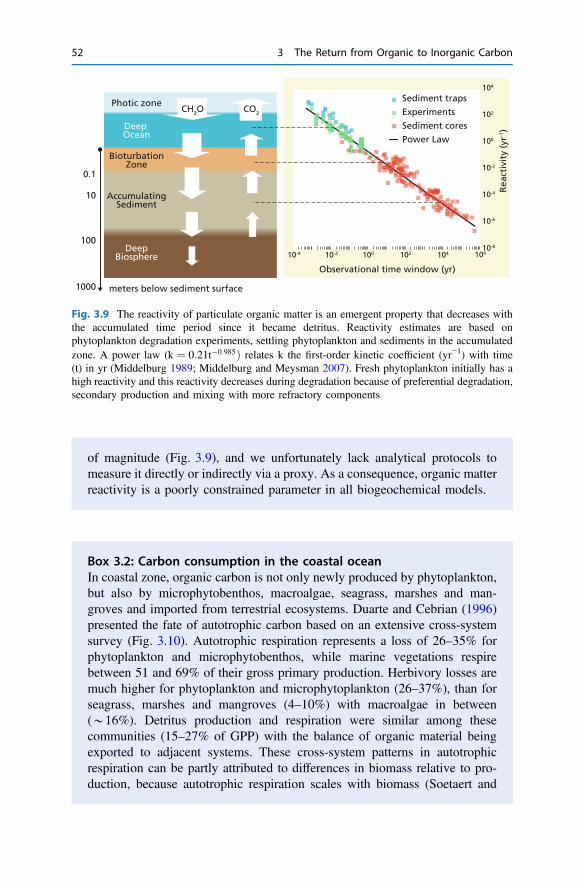
of magnitude (Fig. 3.9), and we unfortunately lack analytical protocols tomeasure it directly or indirectly via a proxy. As a consequence, organic matterreactivity is a poorly constrained parameter in all biogeochemical models.

Box 3.2: Carbon consumption in the coastal oceanIn coastal zone, organic carbon is not only newly produced by phytoplankton,but also by microphytobenthos, macroalgae, seagrass, marshes and man-groves and imported from terrestrial ecosystems. Duarte and Cebrian (1996)presented the fate of autotrophic carbon based on an extensive cross-systemsurvey (Fig. 3.10). Autotrophic respiration represents a loss of 26–35% forphytoplankton and microphytobenthos, while marine vegetations respirebetween 51 and 69% of their gross primary production. Herbivory losses aremuch higher for phytoplankton and microphytoplankton (26–37%), than forseagrass, marshes and mangroves (4–10%) with macroalgae in between(*16%). Detritus production and respiration were similar among thesecommunities (15–27% of GPP) with the balance of organic material beingexported to adjacent systems. These cross-system patterns in autotrophicrespiration can be partly attributed to differences in biomass relative to pro-duction, because autotrophic respiration scales with biomass (Soetaert and

1000

100

10

0.1

10-8

10-6

10-4

10-2

100

102

104

10-4 10-2 100 102 104 106

Rea

ctiv

ity

(yr-1

)

Observational time window (yr)

Photic zone

DeepBiosphere

BioturbationZone

AccumulatingSediment

Deep Ocean

meters below sediment surface

CH2O CO2

Sediment traps

Experiments

Sediment cores

Power Law

Fig. 3.9 The reactivity of particulate organic matter is an emergent property that decreases withthe accumulated time period since it became detritus. Reactivity estimates are based onphytoplankton degradation experiments, settling phytoplankton and sediments in the accumulatedzone. A power law (k ¼ 0:21t�0:985Þ relates k the first-order kinetic coefficient (yr−1) with time(t) in yr (Middelburg 1989; Middelburg and Meysman 2007). Fresh phytoplankton initially has ahigh reactivity and this reactivity decreases during degradation because of preferential degradation,secondary production and mixing with more refractory components


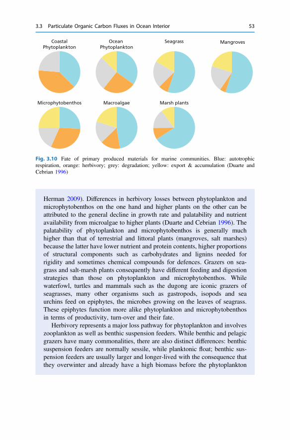
Herman 2009). Differences in herbivory losses between phytoplankton andmicrophytobenthos on the one hand and higher plants on the other can beattributed to the general decline in growth rate and palatability and nutrientavailability from microalgae to higher plants (Duarte and Cebrian 1996). Thepalatability of phytoplankton and microphytobenthos is generally muchhigher than that of terrestrial and littoral plants (mangroves, salt marshes)because the latter have lower nutrient and protein contents, higher proportionsof structural components such as carbohydrates and lignins needed forrigidity and sometimes chemical compounds for defences. Grazers on sea-grass and salt-marsh plants consequently have different feeding and digestionstrategies than those on phytoplankton and microphytobenthos. Whilewaterfowl, turtles and mammals such as the dugong are iconic grazers ofseagrasses, many other organisms such as gastropods, isopods and seaurchins feed on epiphytes, the microbes growing on the leaves of seagrass.These epiphytes function more alike phytoplankton and microphytobenthosin terms of productivity, turn-over and their fate.

Herbivory represents a major loss pathway for phytoplankton and involveszooplankton as well as benthic suspension feeders. While benthic and pelagicgrazers have many commonalities, there are also distinct differences: benthicsuspension feeders are normally sessile, while planktonic float; benthic sus-pension feeders are usually larger and longer-lived with the consequence thatthey overwinter and already have a high biomass before the phytoplankton

Ocean Phytoplankton

CoastalPhytoplankton

MacroalgaeMicrophytobenthos

Seagrass

Marsh plants

Mangroves

Fig. 3.10 Fate of primary produced materials for marine communities. Blue: autotrophicrespiration, orange: herbivory; grey: degradation; yellow: export & accumulation (Duarte andCebrian 1996)


spring bloom. Moreover, benthic suspension feeders have only access tophytoplankton in the lower part of the water column and vertical mixing is animportant factor governing their growth and their impact on phytoplanktondynamics (Herman et al. 1999).

Coastal systems exchange organisms and detrital material with adjacentecosystems and receive detrital resources via rivers. This additional externalorganic matter is consumed and, as a consequence, the local balance betweenautotrophic and heterotrophic processes is disturbed, with net ecosystemheterotrophy as a result (Smith and Hollibaugh 1993). Heterotrophicecosystems often show secondary production, similar to or higher than pri-mary production, a dominance of microbial processes, a depletion in dis-solved oxygen, and high carbon dioxide levels (Heip et al. 1995).

References

Anderson TR, LeB Williams PJ (1998) Modelling the seasonal cycle of dissolved organic carbonat station E1 in the English channel. Estuar Coast Shelf Sci 46:93–109

Andersson H, Wijsman JWM, Herman PMJ, Middelburg JJ, Soetaert K, Heip C (2004)Respiration patterns in the deep ocean. Geophys Res Lett 31. https://doi.org/10.1029/2003gl018756

Arndt S, Jørgensen BB, LaRowe D, Middelburg JJ, Pancost R, Regnier P (2013) Quantification oforganic matter degradation in marine sediments: a synthesis and review. Earth Sci Rev 123:53–86

Azam F, Fenchel T, Field JG, Gray JS, Meyer-Reil LA, Thingstad F (1983) The ecological role ofwater-column microbes in the sea. Mar Ecol-Prog Ser 10:257–263

Berelson W (2001) POC fluxes into the ocean interior: a comparison of 4 US-JGOFS regionalstudies. Oceanography 14:59–67

Berelson WM (2002) Particle settling rates increase with depth in the ocean. Deep Sea Res II,49:237–251

Berner RA (1964) An idealized model of dissolved sulfate distribution in recent sedimentsGeochimica et Cosmochimica Acta 28:1497–1503

Bossata E, Ågren GI (1995) The power and reactive continuum models as particular cases of theq-theory of organic matter dynamics. Geochimica et Cosmochimica Acta 59:3833–3835

Boudreau BP, Ruddick BR (1991) On a reactive continuum representation of organic matterdiagenesis. Am J Sci 291:507–538

Clegg SL, Whitfield M (1990) A generalized model for the scavenging of trace metals in the openocean. I.—Particle cycling. Deep-Sea Res 37:809–832

Dauwe B, Middelburg JJ, Herman PMJ, Heip CHR (1999) Linking diagenetic alteration of aminoacids and bulk organic matter reactivity. Limnol Oceanogr 44:1809–1814

Duarte CM, Cebrian J (1996) The fate of marine autotrophic production. Limnol Oceanogr41:1758–1766

Dugdale RC, Goering JJ (1967) Uptake of new and regenerated forms of nitrogen in primaryproductivity. Limnol Oceanogr 12:196–206


http://dx.doi.org/10.1029/2003gl018756

http://dx.doi.org/10.1029/2003gl018756

Dunne JP, Sarmiento JL, Gnanadesikan A (2007) A synthesis of global particle export from thesurface ocean and cycling through the ocean interior and on the seafloor. Glob BiogeochemCycles 21:GB4006. https://doi.org/10.1029/2006gb002907

Dunne JP, Armstrong RA, Gnanadesikan A, Sarmiento JL (2005) Empirical and mechanisticmodels for the particle export ratio. Global Biogeochem Cycles 19:GB4026. https://doi.org/10.1029/2004gb002390

Field CB, Behrenfeld MJ, Randerson JT, Falkowski PG (1998) Primary production of thebiosphere: integrating terrestrial and oceanic components. Science 281:237–240

Glud RN (2008) Oxygen dynamics of marine sediments. Mar Biol Res 4:243–289Heip CHR, Goosen NK, Herman PMJ, Kromkamp J, Middelburg JJ, Soetaert K (1995) Production

and consumption of biological particles in temperate tidal estuaries. Oceanogr Mar Biol AnnRev 33:1–150

Herman PMJ, Middelburg JJ, van de Koppel J, Heip CHR (1999) Ecology of estuarinemacrobenthos. Adv Ecol Res 29:195–240

Jørgensen BB (1978) A comparison of methods for the quantification of bacterial sulfate reductionin coastal marine sediments. II. Calculation from mathematical models. Geomicrobiol J 1:29–47

Laws EA, D’Sa E, Puneeta N (2011) Simple equations to estimate ratios of new or exportproduction to total production from satellite‐derived estimates of sea surface temperature andprimary production. Limnol Oceanogr Methods 9. https://doi.org/10.4319/lom.2011.9.593

Laws EA, Falkowski PG, Smith WO, Ducklow H, McCarthy JJ (2000) Temperature effects onexport production in the open ocean. Glob Biogeochem Cycles 14:1231–1246

Legendre L, Rassoulzadegan F (1995) Plankton and nutrient dynamics in marine waters. Ophelia41:153–172

Lutz M, Dunbar R, Caldeira K (2002) Regional variability in the vertical flux of particulate organiccarbon in the ocean interior. Glob Biogeochem Cycles 16:1037. https://doi.org/10.1029/2000GB001383

Martin JH, Knauer GA, Karl DM, Broenkow WW (1987) VERTEX: carbon cycling in theNortheast Pacific. Deep Sea Res 34:267–285

Middelburg JJ (1989) A simple rate model for organic-matter decomposition in marine sediments.Geochim Cosmochim Acta 53:1577–1581

Middelburg JJ, Meysman FJR (2007) Burial at sea. Science 317:1294–1295Pace ML, Cole JJ, Carpenter SR, Kitchell JF (1999) Trophic cascades revealed in diverse

ecosystems. Trends Ecol Evol 14:483–488Pace ML, Knauer GA, Karl DM, Martin JH (1987) Primary production, new production and

vertical flux in the Eastern Pacific Ocean. Nature 325:803–804Sarmiento J, Gruber N (2006) Ocean biogeochemical dynamics. Princeton University Press,

Princeton, p 526Smith SV (1981) Marine macrophytes as a global carbon sink. Science 211:838–840Smith SV, Hollibaugh JT (1993) Coastal metabolism and the oceanic organic carbon balance. Rev

Geophys 31:75–89Soetaert K, Herman PMJ (2009) A practical guide to ecological modelling. Springer, Netherlands,

p 372Suess E (1980) Particulate organic carbon flux in the oceans-surface productivity and oxygen

utilization. Nature 288:260–263Suttle CA (2005) Viruses in the sea. Nature 437:356–361Van den Meersche K, Middelburg JJ, Soetaert K, van Rijswijk P, Boschker HTS, Heip CHR

(2004) Carbon–nitrogen coupling and algal–bacterial interactions during an experimentalbloom: modeling a 13C tracer experiment. Limnol Oceanogr 49:862–878

References 55

http://dx.doi.org/10.1029/2006gb002907

http://dx.doi.org/10.1029/2004gb002390

http://dx.doi.org/10.1029/2004gb002390

http://dx.doi.org/10.4319/lom.2011.9.593

http://dx.doi.org/10.1029/2000GB001383

http://dx.doi.org/10.1029/2000GB001383

Volk T, Hoffert MI (1985) Ocean carbon pumps: analysis of relative strengths and efficiencies inocean-driven atmospheric CO2 change. In: Sundquist ET, Broecker WS (eds) The Carboncycle and atmospheric CO2: natural variations Archean to present. AGU, Washington, pp 99–110

Westrich JT, Berner RA (1984) The role of sedimentary organic matter in bacterial sulfatereduction: the G model tested. Limnol Oceanogr 29:236–249

Yamanaka Y, Tajika E (1996) The role of the vertical fluxes of particulate organic matter andcalcite in the oceanic carbon cycle: studies using an ocean biogeochemical general circulationmodel. Global Biogeochem Cycles 10:361–382





4Carbon Processing at the Seafloor

Most of the global marine primary production (*55 Pg C y−1) is consumed in thesurface, sunlit ocean (*44 Pg C y−1) and ocean interior (*8 Pg C y−1) and onlythe remaining 2–3 Pg C y−1 reaches the sediment floor. Globally most of theorganic carbon delivered to sediments (*90%) is degraded because organic carbonburial is low (*0.2–0.4 Pg C y−1) and mainly occurs in rapidly accumulatingcoastal sediments.

In this chapter, we will first discuss organic matter delivery to the sediments,then the processes and organisms involved in organic matter degradation and closewith a discussion of factors governing organic carbon burial.

4.1 Organic Matter Supply to Sediments

In Chap. 3 we have seen that organic carbon deposition on the seafloor dependsprimarily on water depth (Fig. 3.4), as a direct consequence of organic matterproduction in the euphotic zone and degradation of detritus during transit from thesunlit layer to the bottom of the ocean with more time for degradation in deep-watersettings than in coastal settings. Consequently, deep-sea sediments receive littleorganic matter, while coastal sediments receive much. This water depth dependencyof organic matter delivery rates is articulated by lateral differences in ocean primaryproduction (production in shallow coastal systems is generally higher than that inthe open ocean). Marine sediments are therefore often considered donor-controlled,i.e. the organic matter consuming benthic communities have no control over theirfood resources. While such a donor-controlled view applies to most deep-seaenvironments, there are other carbon delivery routes for sediments within theeuphotic zone and for sediments inhabited by animals and these carbon transfers tosediments are (partly) mediated by the consuming communities, i.e. under con-sumer control (Fig. 4.1; Middelburg 2018).


57




https://doi.org/10.1007/978-3-030-10822-9_4

Intertidal sediments and coastal sediments within the euphotic zone may supportmicrobial photoautotrophs (microphytobenthos). Gattuso et al. (2006) showed thatglobally about 1/3 of sediments within the coastal ocean receive sufficient light forphotosynthesis. This primary production at the seafloor represent a sourceof *0.32 Pg C yr−1 that is not only directly available for consumption, but it is alsoof high quality, because there has been no pre-depositional processing of organicmatter. This benthic primary production input thus supports about 10–15% ofglobal sediment respiration. Moreover, the grazing by micro, meio and macrofaunacontrols the biomass of the primary producers and in this way grazing animalscontrol food supply for themselves, as well as for microbes living on the exudatesand detritus of microphytobenthos (Middelburg et al. 2000; Middelburg 2018).

Macrophytes such as seagrasses in the subtidal euphotic zone and marsh plantsand mangroves in the intertidal zone enhance carbon inputs to sediments in twoways. They locally produce new organic matter that is used for respiration, investedin leaves and stems, allocated to below-ground tissues for nutrient (and water)uptake, anchoring and storage. All this tissue can be consumed by microbes andanimals, although the degradability of structural carbohydrate rich macrophytematerial is often lower than that of protein-rich microphytobenthos and phyto-plankton material (Duarte and Cebrian 1996; Fig. 3.10). Macrophyte communitiesstabilize the sediments and impact the local hydrodynamics with the consequencethat suspended particles, including particulate organic matter, are trapped within

POC

POC

DOC

(1) Donor control

(3) Incorporation of labile carbon at surface

(2) Consumer control in photic zone

(4) Suspension feeders and biodeposition

(5) Sponge loop

Grazing herbivores impact C supply

Bioturbating animals transfer C down the gradient

Fig. 4.1 Organic matter supply to sediments (Middelburg 2018). (1) Organic matter settling fromthe water column is deposited at seafloor (donor control; fixed flux upper boundary condition).(2) Sediments in the photic zone are inhabited by benthic microalgae that produce new organicmatter in situ and grazing animals can impact the growth of these primary producers.(3) Bioturbating animals transfer labile carbon from the sediment surface layer to deeper layersin the sediments. (Vertical axis is depth; horizontal axis is concentration, see Fig. 4.2)(4) Suspension-feeding organisms enhance the transfer of suspended particulate matter from thewater column to the sediments (biodeposition). (5) Sponge consume dissolved organic carbon andproduce cellular debris that can be consumed by benthic organisms (i.e., the sponge loop)

58 4 Carbon Processing at the Seafloor

their canopies. This trapped organic matter is often derived from adjacent ecosys-tems or phytoplankton from within the system and makes a substantial contributionto sediment organic carbon pools in salt marshes (Middelburg et al. 1997) andseagrass meadows (Gacia et al. 2002; Kennedy et al. 2010). Moreover, the trappedphytodetritus often is more readily degradable than locally produced macrophytematerial (Barrón et al. 2006).

Suspension feedings worms, bivalves, corals and sponges consume particulateorganic matter suspended in the water column. Part of the carbon is used for growthand maintenance, another part is excreted as faeces and pseudofaeces, which in turnare available for microbes and animals in the underlying and nearby sediments.Some organisms passively filter water, whereas others actively filter water to obtaintheir resources. Clearance rates (m3 of water cleared from food per unit time) can bevery high, and grazing by benthic suspension feeders often represents the largestloss term of phytoplankton in tidal systems (Heip et al. 1995). While some sus-pension feeders are spatially distributed rather homogenously, many others (e.g.oysters, mussels, coral reefs) occur in specific areas at high densities because oflocal favourable hydrodynamic conditions or positive feedbacks between commu-nity density, performance and local hydrodynamics (Herman et al. 1999). Thesesuspension feeders locally enhance carbon input to underlying sediments relative tothat delivered via sinking because they focus laterally available particulate organiccarbon. Some of the highest carbon inputs to sediments have been reported formussel and oyster beds. Moreover, benthic suspension feeders within the euphoticzone directly impact phytoplankton growth and dynamics (Koseff et al. 1993).

Sandy sediments cover about 50% of the continental shelf seafloor and about 4%of the total ocean floor. Their high permeability allows flow of water through theconnected pore network of these sediments. These flows are driven by current orwave induced pressure differences, which may be enhanced through biologicalstructures. Active flows of seawater with suspended particles result in additionaltransport of particulate organic matter to sediments. Part of the suspended partic-ulate matter entering into these sediments with the water is trapped or utilized byorganisms (Huettel et al. 2014), thus supplementing the particulate organic mattersupply to these sediments. This additional organic carbon is highly reactive, andparticulate organic carbon stocks in permeable sediments are very low (Boudreauet al. 2001).

Another organic carbon provision pathway to sediments involves organisms thatconsume dissolved organic carbon and use it to form particulate organic carbon(biomass and excretion products), which can be used by other consumers living atthe sediment-water interface or within the sediments. This mechanism has beendocumented for encrusting sponges that consume large quantities of dissolvedorganic carbon and rapidly convert this into detritus for benthic consumers (i.e.sponge loop, de Goeij et al. 2013).

It is important to realize that some of these additional pathways involve trulynew organic carbon (benthic primary production), while the others either convertwidely available, but poorly useable, dissolved organic carbon into a particulatepool (sponge loop) or focus particulate organic matter delivered to a wide area for

4.1 Organic Matter Supply to Sediments 59

deposition into small areas inhabited by suspension feeding animals or plants. Thelatter category locally enhances organic matter decomposition at the expense ofadjacent areas or water-column degradation. Finally, even in donor-controlledsediments, animals enhance the transfer of labile organic matter to subsurfacemicrobial communities by bioturbation (Box 4.1) and in that way stimulate theoverall degradation of organic matter (Middelburg 2018). This mechanism will bepresented in detail below; we will first introduce the consuming organisms.

4.2 The Consumers

Organic matter delivered to the sediments represents the major resource for theheterotrophic consumers living in the sediments. These organic carbon consumersare usually partitioned into size classes: microbenthos (<32 lm), meiobenthos (32lm–0.5/1 mm) and macrobenthos (>0.5/1 mm), the actual size class divisiondepending on the environment (smaller for deep-sea than coastal studies). Themicrobenthos includes small eukaryotes (Protists), but is by far dominated byprokaryotes (Bacteria and Archaea). The meiobenthos is often dominated bynematodes, but foraminifera (protists) also contribute. The macrobenthos comprisesmany different animal groups. The number of organisms declines with size: from109 bacteria per ml of sediments (i.e. 1014 cells in the top 10 cm of 1 m2), 106

meiofauna m−2 to 104 macrofauna m−2 in estuarine sediments (Herman et al. 1999).The distances between individuals is thus of the order 10 lm, 1 mm and 1 cm formicrobes, meiofauna and macrofauna, respectively. Microbes are much smallerthan typical pore sizes of silty and sandy sediments, meiofauna can live within thesepores, while macrofauna are much larger and consequently move particles whenactive. The mixing of particles and solutes by animals living in sediment is calledbioturbation (Box 4.1) and has major consequences for carbon processing in sed-iments (Meysman et al. 2006; Middelburg 2018).

The organic carbon consumed by benthic heterotrophs is used for maintenance,growth and reproduction. The relative importance of the different size classes tocarbon consumption scales more or less with their contribution to biomass. Incoastal sediments, macrofauna typically accounts for 10–25% of the total biomassand respiration, with microbes accounting for the remaining, except for a small (few%) contribution of protists and meiofauna. Macrofauna number and size (and thusbiomass) decline stronglywith water depth compared to those of meiofauna and inparticular microbes (Snelgrove et al. 2018). Carbon consumption in deep-seasediments is almost entirely due to microbes. Accordingly, organic matter con-sumption is normally attributed to sedimentary microbes, and the consumption oforganic matter by animals is therefore ignored in most biogeochemical studies(Middelburg 2018).


4.3 Organic Carbon Degradation in Sediments

Organic carbon degradation in sediments is a highly efficient process because mostof the incoming organic carbon is degraded and only a small fraction eventuallyescapes mineralization to be buried with the accumulating sediments. This fractionis often quantified in terms of the burial efficiency (BE):

BE ¼ FB

FC¼ FB

FB þRð Þ ð4:1Þ

where FC is the incoming carbon flux, FB is the rate of carbon burial and R is thetotal mineralization rate. Burial efficiencies are often presented as a percentage andrange from a fraction of a percent in deep-sea sediments up to tens of a percent inrapidly accumulating coastal sediments (Canfield 1994; Aller 2013). In mostoceanic sediments, R >> FB, and total respiration is a reliable proxy for quantifyingthe organic carbon delivery rate to sediments (FC).

This high efficiency of organic matter degradation within in sediments mightseem paradoxical because sediments receive organic matter that has already beenprocessed extensively before deposition. Pre-depositional processing of organicmatter not only lowers the amount of organic matter delivered, but also the qualitybecause of the preferential use of labile organic carbon by organisms (Fig. 3.9).However, when particulate organic matter is transferred from the water column,with a typical residence time of weeks to months, to the top layer of sediments, thetime available for degradation changes by orders of magnitude (103–104 years).This increase in time available for processing organic matter more than compen-sates for the loss of reactivity during particle settling; hence, organic matterdegradation resumes.

To understand the dynamics and distribution of organic matter in sediments wewill again use the simple diffusion-advection-reaction model introduced in Box 1.1.Modelling the distribution and dynamics of organic carbon in sediments is ratherchallenging because the transport of organic carbon, as well as its production andconsumption, are biologically controlled, and we cannot resort to physics-basedlaws for transport. Moreover, we are dealing with a two-phase problem (particlesand water). The first simplification is that we only consider particulate organiccarbon. For a sediment with a porosity (volume water/total volume) of 0.7, aparticulate organic carbon content of 1 wt% and a very high pore-water dissolvedorganic carbon concentration (1 mM), dissolved organic carbon contributes about1‰ to the sediment carbon stock. Moreover, the reactivity of dissolved organiccarbon is relative low. Two, gradients in porosity due to compaction and biotur-bation are ignored. Three, organic carbon degradation follows first-order kinetics(one-G model, Berner 1964; Box 3.1). Four, electron acceptors are abundant andtheir nature does not impact organic carbon degradation. Five, solid-phase organiccarbon is transported by bioturbation (Box 4.1) and by the net accretion ofsediment.

4.3 Organic Carbon Degradation in Sediments 61

Transport of particulate organic carbon due to animal activity is the dominanttransport process in sediment inhabited by animals. The transport resulting frombioturbation can usually be well described by diffusion (Goldberg and Koide 1962;Berner 1980), in particular when the benthic community is diverse (Meysman et al.2006, 2010). It is only in sediments where chemical conditions (e.g. lack of oxygen,pollution) or physical conditions (e.g. unstable sediments that are repetitively dis-turbed by waves/tides) restrict macrofauna that bioturbation can be ignored andorganic carbon transport due to sediment accretion dominates. Finally by assumingsteady-state, the resulting equation for organic carbon (G) is:

0 ¼ Dbd2G

dx2� w

dG

dx� kG ð4:2Þ

where G is labile particulate organic carbon, x is depth (positive downwards), Db isthe bioturbation coefficient (cm2 yr−1), w is the sediment accumulation rate (cmy−1) and k is a first-order rate constant (yr−1). Considering that all labile organiccarbon is eventually consumed (at depth), we can solve the equation for specificconditions at the sediment-water interface (x = 0). It is instructive to distinguishbetween sediments that are strictly donor-controlled (i.e. a fixed flux upperboundary) and sediments with a fixed concentration in the top layer. The formerapplies to most sediments, while the latter would represent coastal sediments withmultiple deposition–resuspension events and lateral particulate organic transportpathways (Rice and Rhoads 1989). If we know the concentration of organic carbonat the sediment-water interface (G0), the solution is (see Box 1.1):

G ¼ G0eax with a ¼ w� ffiffiffiffiffiffiffiffiffiffiffiffiffiffiffiffiffiffiffiffiffi

w2 þ 4kDb

p

2Dbð4:3Þ

Alternatively, if the flux of organic carbon delivered to the sediment (F) is knownthe solution is:

G ¼ F

�Dbaþweax; ð4:4Þ

where a is the same as in Eq. 4.3.Figure 4.2 shows the distribution of organic carbon as a function of sediment

depth, for a fixed reactivity and sediment accumulation rate, and for differentbioturbation coefficients. The distribution of organic carbon declines exponentially

with depth and the attenuation is to a first-approximation governed byffiffiffiffikDb

q, i.e.

more mixing (higher Db) will flatten organic carbon concentration versus depthprofiles (because the contribution of w to the attenuation coefficient a is very small).In other words, particle mixing by moving animals will transfer organic carbon tolarger depths. This is articulated in sediments with a fixed concentration in the toplayer. For these sediments bioturbation will increase the total amount of organic


matter available for the benthic community. In other words, animals have, to acertain extent, control over their food supply. The other major factor governingorganic matter profiles in sediments is the reactivity of organic matter. Morereactive organic matter is degraded shallower and does not penetrate as deep intothe sediment as refractory organic matter (Fig. 4.3). Moreover, the inventory oforganic carbon in surface sediments is higher when the reactivity of organic matteris lower, in particular for a fixed amount of carbon supplied per unit time.

Evidently, when applying this type of models, it is important to select theappropriate upper boundary conditions. While deep-sea sediments can best bedescribed by an organic carbon flux boundary condition, the proper upper boundarycondition for coastal sediments is not clear. A fixed concentration upper boundaryconditions may be more appropriate for shelf systems in which lateral organiccarbon fluxes dominate, e.g. due to a combination of resuspension-depositioncycles and residual tidal flow. Animals collecting organic matter in the surfacesediment layer and bioturbating it to deeper layers make thus additional organicmatter of high quality available to microbes. Moreover, first-order reactivity

0

1

2

3

4

5

6

7

8

9

10

0 10 20 30 40 50 0 10 20 30 40 50

Dep

th (

cm)

Corg (mg C g-1) Corg (mg C g-1)

9529D 0.1D 1D 10D100

Fig. 4.2 Organic carbon concentration versus depth profiles for different bioturbation coefficients(0.1, 1, 10, 100 cm2 yr−1) for a fixed concentration of 20 mg C gr−1 (left) and a fixed flux of36 mg C cm−2 yr−1 (right). The imposed flux has been tuned to generate an identical concentrationat the sediment-water interface for a Db of 10 cm2 yr−1. Model parameters: k = 1 yr−1;w = 0.1 cm yr−1


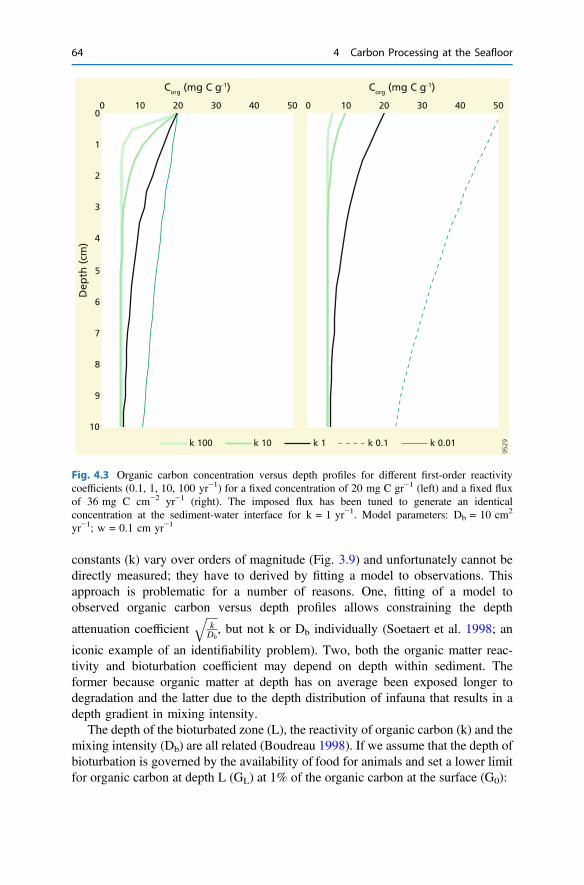
constants (k) vary over orders of magnitude (Fig. 3.9) and unfortunately cannot bedirectly measured; they have to derived by fitting a model to observations. Thisapproach is problematic for a number of reasons. One, fitting of a model toobserved organic carbon versus depth profiles allows constraining the depth

attenuation coefficientffiffiffiffikDb

q, but not k or Db individually (Soetaert et al. 1998; an

iconic example of an identifiability problem). Two, both the organic matter reac-tivity and bioturbation coefficient may depend on depth within sediment. Theformer because organic matter at depth has on average been exposed longer todegradation and the latter due to the depth distribution of infauna that results in adepth gradient in mixing intensity.

The depth of the bioturbated zone (L), the reactivity of organic carbon (k) and themixing intensity (Db) are all related (Boudreau 1998). If we assume that the depth ofbioturbation is governed by the availability of food for animals and set a lower limitfor organic carbon at depth L (GL) at 1% of the organic carbon at the surface (G0):

0

1

2

3

4

5

6

7

8

9

10

0 10 20 30 40 50 0 10 20 30 40 50

Corg (mg C g-1) Corg (mg C g-1)D

epth

(cm

)

9529k 100 k 10 k 1 k 0.01k 0.1

Fig. 4.3 Organic carbon concentration versus depth profiles for different first-order reactivitycoefficients (0.1, 1, 10, 100 yr−1) for a fixed concentration of 20 mg C gr−1 (left) and a fixed fluxof 36 mg C cm−2 yr−1 (right). The imposed flux has been tuned to generate an identicalconcentration at the sediment-water interface for k = 1 yr−1. Model parameters: Db = 10 cm2

yr−1; w = 0.1 cm yr−1


GL

G0¼ 0:01 ¼ e

ffiffiffiffi�kDb

pL ð4:5Þ

Making use of ln(0.01) � 4.6, this equation can be re-arranged to

L ¼ 4:6

ffiffiffiffiffiffiDb

k

r: ð4:6Þ

The depth of the mixed layer is thus directly related the reactivity of the organicmatter and the mixing intensity. This equation is highly similar to the more elab-

orate result of Boudreau (1998) L ¼ 4ffiffiffiffiffiffi9Db8k

qthat is based on a resource-feedback

model. Figure 4.4 shows the depth of the bioturbated zone as a function of organicmatter reactivity and bioturbation intensity. The observed range of Db and k inmarine sediments is also indicated. Bioturbation depth in marine sediments varybetween 1 and 20 cm, with a global average of about 10 cm (Boudreau 1998). Thiscan be obtained either by high mixing, if organic matter is highly reactive as incoastal sediments, or by low mixing, with less reactive matter in the deep sea.

4.4 Consequences for Sediment Biogeochemistry

Degradation of organic carbon to inorganic carbon requires an electron acceptor, e.g.oxygen. In the water column, oxygen supply is usually sufficient to accept all electronreleased during respiration, but in sediments solutes such as oxygen are transportedprimarily by molecular diffusion, and oxygen supply rates often do not match oxygenconsumption rates with the consequence that most sediments become anoxic at somedepth. In the absence of oxygen, organic matter is either respired anaerobically orfermented. Fermentation refers to an internal redistribution of electrons among carbonatoms with the result that carbon dioxide and methane are formed.

2CH2O ) CO2 þ CH4

Anaerobic respiration and fermentation of particulate organic matter involvesmultiple steps in a complex network: hydrolysis and fermentation of larger mole-cules to smaller molecules and finally the use of alternative electron acceptors(Jørgensen 2006). These intermediate products include short-chain fatty acids suchas formate, acetate, propionate and butyrate, and hydrogen. The latter has a highturn-over (minutes) because of rapid production and consumption, e.g. duringhydrogenotrophic processes such as carbon dioxide reduction to methane (e.g.Beulig et al. 2018).


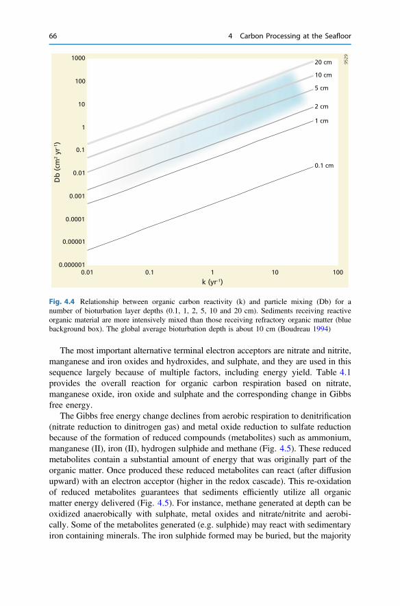
The most important alternative terminal electron acceptors are nitrate and nitrite,manganese and iron oxides and hydroxides, and sulphate, and they are used in thissequence largely because of multiple factors, including energy yield. Table 4.1provides the overall reaction for organic carbon respiration based on nitrate,manganese oxide, iron oxide and sulphate and the corresponding change in Gibbsfree energy.

The Gibbs free energy change declines from aerobic respiration to denitrification(nitrate reduction to dinitrogen gas) and metal oxide reduction to sulfate reductionbecause of the formation of reduced compounds (metabolites) such as ammonium,manganese (II), iron (II), hydrogen sulphide and methane (Fig. 4.5). These reducedmetabolites contain a substantial amount of energy that was originally part of theorganic matter. Once produced these reduced metabolites can react (after diffusionupward) with an electron acceptor (higher in the redox cascade). This re-oxidationof reduced metabolites guarantees that sediments efficiently utilize all organicmatter energy delivered (Fig. 4.5). For instance, methane generated at depth can beoxidized anaerobically with sulphate, metal oxides and nitrate/nitrite and aerobi-cally. Some of the metabolites generated (e.g. sulphide) may react with sedimentaryiron containing minerals. The iron sulphide formed may be buried, but the majority

0.000001

0.00001

0.0001

0.001

0.01

0.1

1

10

100

1000

0.01 0.1 1 10 100

Db

(cm

2 yr

-1)

k (yr-1)

9529

20 cm

10 cm

5 cm

2 cm

1 cm

0.1 cm

Fig. 4.4 Relationship between organic carbon reactivity (k) and particle mixing (Db) for anumber of bioturbation layer depths (0.1, 1, 2, 5, 10 and 20 cm). Sediments receiving reactiveorganic material are more intensively mixed than those receiving refractory organic matter (bluebackground box). The global average bioturbation depth is about 10 cm (Boudreau 1994)


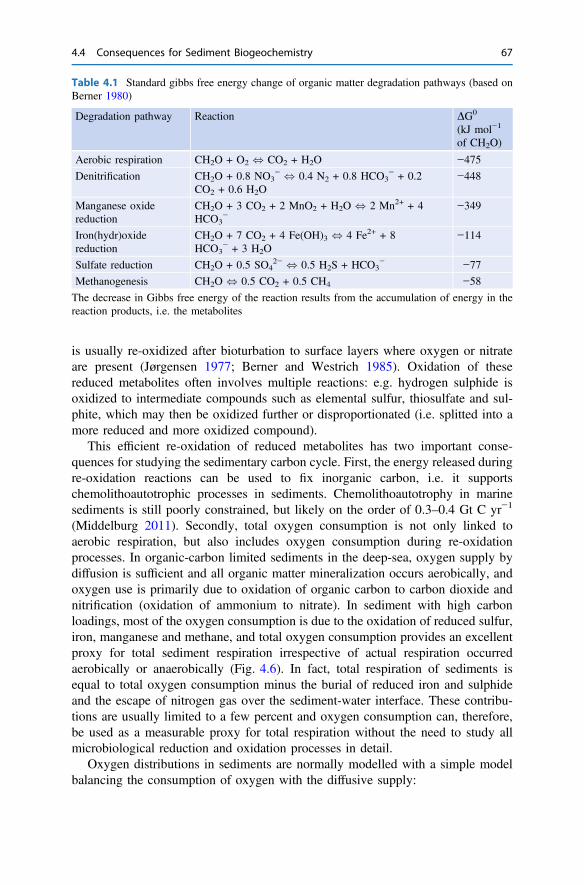
is usually re-oxidized after bioturbation to surface layers where oxygen or nitrateare present (Jørgensen 1977; Berner and Westrich 1985). Oxidation of thesereduced metabolites often involves multiple reactions: e.g. hydrogen sulphide isoxidized to intermediate compounds such as elemental sulfur, thiosulfate and sul-phite, which may then be oxidized further or disproportionated (i.e. splitted into amore reduced and more oxidized compound).

This efficient re-oxidation of reduced metabolites has two important conse-quences for studying the sedimentary carbon cycle. First, the energy released duringre-oxidation reactions can be used to fix inorganic carbon, i.e. it supportschemolithoautotrophic processes in sediments. Chemolithoautotrophy in marinesediments is still poorly constrained, but likely on the order of 0.3–0.4 Gt C yr−1

(Middelburg 2011). Secondly, total oxygen consumption is not only linked toaerobic respiration, but also includes oxygen consumption during re-oxidationprocesses. In organic-carbon limited sediments in the deep-sea, oxygen supply bydiffusion is sufficient and all organic matter mineralization occurs aerobically, andoxygen use is primarily due to oxidation of organic carbon to carbon dioxide andnitrification (oxidation of ammonium to nitrate). In sediment with high carbonloadings, most of the oxygen consumption is due to the oxidation of reduced sulfur,iron, manganese and methane, and total oxygen consumption provides an excellentproxy for total sediment respiration irrespective of actual respiration occurredaerobically or anaerobically (Fig. 4.6). In fact, total respiration of sediments isequal to total oxygen consumption minus the burial of reduced iron and sulphideand the escape of nitrogen gas over the sediment-water interface. These contribu-tions are usually limited to a few percent and oxygen consumption can, therefore,be used as a measurable proxy for total respiration without the need to study allmicrobiological reduction and oxidation processes in detail.

Oxygen distributions in sediments are normally modelled with a simple modelbalancing the consumption of oxygen with the diffusive supply:

Table 4.1 Standard gibbs free energy change of organic matter degradation pathways (based onBerner 1980)

Degradation pathway Reaction DG0

(kJ mol−1

of CH2O)

Aerobic respiration CH2O + O2 , CO2 + H2O −475

Denitrification CH2O + 0.8 NO3− , 0.4 N2 + 0.8 HCO3

− + 0.2CO2 + 0.6 H2O

−448

Manganese oxidereduction

CH2O + 3 CO2 + 2 MnO2 + H2O , 2 Mn2+ + 4HCO3

−−349

Iron(hydr)oxidereduction

CH2O + 7 CO2 + 4 Fe(OH)3 , 4 Fe2+ + 8HCO3

− + 3 H2O−114

Sulfate reduction CH2O + 0.5 SO42− , 0.5 H2S + HCO3

− −77

Methanogenesis CH2O , 0.5 CO2 + 0.5 CH4 −58

The decrease in Gibbs free energy of the reaction results from the accumulation of energy in thereaction products, i.e. the metabolites

4.4 Consequences for Sediment Biogeochemistry 67

9529

OM

Burial

N2

Mn(II)

Fe(II)

H2S

CH4

Aerobic Respiration

NO3reduction

Mn(IV) reduction

Fe(III) reduction

SO4reduction

CH4formation

Fermentation

Hydrolysis

PO4

NH4

CO2

Deposition

Fig. 4.5 Conceptual model of organic matter (OM) degradation and reoxidation pathways (basedon Jørgensen 2006, and Middelburg and Levin 2009). The red arrows reflect the fate of(energy-rich) substrates released during anaerobic mineralization

9529

Sed

imen

t D

epth

SO42- H2S

CO2Corg

O2H2O

O2

penetration depth

Fig. 4.6 Conceptual model of tight coupling sulfate utilization for respiration of organic carbonand sulphide oxidation by oxygen, with the net result that one mole of oxygen use correspondswith one mole of organic carbon oxidized to carbon dioxide (after Aller 1994)


Dsd2O2

dx2¼ R0 ð4:7Þ

where O2 is the oxygen concentration, Ds is the diffusion coefficient of oxygen insediments and R0 is the consumption of oxygen. Oxygen consumption rates can bedescribed with a depth and oxygen concentration independent rate becausere-oxidation is the dominant oxygen sink. The solution for this zero-order kineticsequation with a fixed concentration at the sediment-water interface (C0) is(Bouldin 1968):

C ¼ R0

2Dsx2 �

ffiffiffiffiffiffiffiffiffiffiffiffiffi2C0R0

Ds

r� �xþC0 ¼ C0 1� x

d

� �2ð4:8Þ

where d is the oxygen penetration depth:

d ¼ffiffiffiffiffiffiffiffiffiffiffiffiffi2C0Ds

R0

rð4:9Þ

This relation shows that the oxygen penetration depth is inversely related to the totalrespiration. High respiration rates in coastal sediment result in shallow oxygen pen-etration (mm scale), while low respiration rates in organic carbon starved deep-seasediments allow oxygen penetration to meters (Fig. 4.7). Moreover, oxygen pene-tration depth exhibits a square-root dependence on bottom-water oxygen levels (C0).

0.001

0.01

0.1

1

10

100

0.01 0.1 1 10 100 1000

Oxy

gen

co

nsu

mp

tio

n (

mo

l m-2 y

r-1)

Oxygen Penetration Depth (cm)

9529

Coastal

Ocean Margin

Deep Sea

Fig. 4.7 The relationship between oxygen consumption and oxygen penetration depth. Highfluxes of oxygen into sediments imply shallow penetration. Oxygen penetration variesfrom <1 mm in coastal sediments to >1 m in deep-sea sediment receiving low carbon loadings

4.4 Consequences for Sediment Biogeochemistry 69

4.5 Factors Governing Organic Carbon Burial

Following active carbon degradation in the water column and continued mineral-ization in surface sediments, at some depth in the sediment all labile organic matterhas been utilized and a background level of organic carbon remains (Figs. 4.2 and4.3). This organic carbon is buried down with the accretion of sediments. Organiccarbon burial is, thus, the product of sediment accumulation and organic carboncontent:

FB ¼ w 1� /ð ÞqsG ð4:10Þ

where w is the sediment accumulation rate (cm yr−1), / is the porosity, qs is the drydensity (gr cm−3), G is the concentration of organic carbon (g C gr−1), with FBexpressed in g C cm−2 yr−1. It is important to realize that w refers to the long-termaccumulation rate at depth and not the rate of sediment deposition at the surface.The concentration of organic carbon should theoretically be at the depth where nofurther degradation occurs. Such a depth would not exist if organic matter decayfollows a reactive continuum: organic matter is reactive on all timescale. However,in most sediments organic carbon concentration rapidly declines with depth andthen remains almost invariant. The precise reference depth is not so important aslong the gradient can be neglected.

Differences in organic carbon burial are primarily determined by differences insediment accumulation and carbon contents, and only secondarily by differences inporosity and density. Sediment porosities vary 0.4–0.8 and dry sediment densitiesfrom 2.6 gr cm−3 for mineral to *2.0 gr cm−3 for peaty sediment. Organic carbonconcentrations depend on the carbon input to sediments and the extent of decaybefore burial. Any process that enhances organic carbon input or impedes degra-dation elevates organic carbon concentration at depth and consequently carbonburial. These two factors relate directly to the old discussion on whether high exportproduction (carbon delivery to sediment) or an oxygen related effect on preservationgoverns burial of organic carbon. The idea is that organic matter degradation in thepresence of oxygen is more efficient than without (Box 4.2).

The by far most important factor governing organic carbon burial is the deliveryof inorganic particles that results in sediment accretion. Sediment accumulation inthe ocean vary about four to five orders of magnitude, from less than 0.1 cm perthousand year in the deep-sea to centimetres per year in rapidly accumulatingcoastal sediments (Aller 2013). Most organic carbon burial, therefore, occurs incoastal sediments. An increase in inorganic particle deposition should, in principle,not increase carbon burial, because the organic carbon will just be diluted, butobservations show otherwise. In nature, particulate organic carbon is mainlyassociated with mineral surfaces and the higher the accumulation of minerals, themore mineral surfaces, with associated organic matter, are buried. Vegetated coastalsediments are another site of high organic carbon burial for two reasons. First, thepresence of macrophytes stabilizes sediment and enhances deposition via canopytrapping of particles. Secondly, the net ecosystem carbon balance of these


communities results in the accumulation of plant derived organic matter. The fol-lowing flux balance can be used to investigate the impact of sediment accretion andnet ecosystem production on the burial of organic carbon in vegetated sediments:

w 1� /ð ÞqsCexternal þ qorganicCtoM NEP ¼ w 1� /ð ÞqsCburied ð4:11Þ

where w is sediment accumulation rate (cm yr−1), / is the porosity, qs is the drydensity of bulk sediment (gr cm−3), Cexternal is the concentration of organic carbon(g C gr−1) in deposited sediments remaining after degradation, qorganic is the densityof plant organic material, CtoM converts organic C to organic matter, and Cburied isthe concentration of buried organic matter. Primary production in cordgrass habitatsis very high (*2 kg C m−2 yr−1) with net carbon accretion of *0.3 kg C m−2 yr−1

(Middelburg et al. 1997). If all that cordgrass detritus is retained in the system,marsh sediment accretion would be *0.5 mm per year, not enough for keepingpace with accelerated global sea-level rise (>2 mm per year) and a mineral starved,peaty marsh may therefore drown. The combined effect of enhanced particletrapping and retention and macrophyte derived organic matter are the reason thatvegetated coastal sediments represent a major term in global marine carbon burial,i.e. blue carbon (Duarte 2017).

Box 4.1: BioturbationBioturbation refers to the reworking of sediments (particles and water) duethe activities of organisms, in particular animals (Meysman et al. 2006). Thisreworking has many consequences, including the creation of athree-dimensional, heterogeneous distribution of sediment properties. In fact,this animal induced heterogeneity is clear from sediments deposited duringthe last 0.5 billion years and palaeontologists have therefore named thisperiod Phanerozoic, after the old greek words phanerós (visible) and zōḗ(life). Moreover, the small-scale heterogeneity stimulates biogeochemical andbiological diversity. It also has consequences for porosity, permeability,sediment stability and roughness.

Besides these effects on sediment properties and characteristics, animalactivities have a major impact on the transport of particles and solutes. Par-ticle mixing, bioturbation sensu stricto, occurs through the construction andmaintenance of structures such as burrows and the movement of particleswhile feeding (ingestion and defecation). Particles are moved vertically andhorizontally, but the consequences are usually more prominent verticallybecause most sediment characteristics show strong vertical gradients. Theparticles dispersed may be reactive or unreactive minerals, organic matter aswell as organisms and their cysts, eggs and remains. Many animals constructand live in burrows and ventilate these with overlying oxygenated water forrespiration or food supply. In permeable sediments, this burrow water canenter the sediments and in permeable and non-permeable sediments diffusiveexchange occurs between burrows and adjacent sediments because of

4.5 Factors Governing Organic Carbon Burial 71

concentration gradients. Many animals are involved in particle mixing andventilation. Particle mixing is pivotal for optimal functioning of sediments:organic matter and solid-phase oxidants such as iron oxides are mixeddownwards, while reduced substance such as iron sulphides are mixedupwards. Bio-irrigation enhances exchange of oxygen, nutrients and othersubstances between water and sediment.

Particle mixing is the result of multiple activities of a diverse assemblageof large animals. While the behaviour of certain species may cause a distinctparticle transport pattern, the net result of many particle mixing events cannormally be described very well as diffusion. Bioturbation is then quantifiedin terms of a biodiffusion coefficient for particles (Db; cm2 yr−1). Thisbiodiffusion coefficient can be derived from modelling concentration versusdepth profiles of a tracer A with a known reactivity (e.g. radioactive decay).Equation 4.12 balances transport due to sediment accumulation and biodif-fusion with radioactive decay at steady state:

0 ¼ Dbd2A

dx2� w

dA

dx� kA ð4:12Þ

where w is the sediment accumulation rate (cm yr−1) and k is the radioactivedecay constant (yr−1). These macroscopic empirical Db values can bedecomposed into discrete particle properties step length (k) and the periodbetween two displacements (s) (Meysman et al. 2010):

Db ¼ k2

2sð4:13Þ

The step length of particle displacement scales with organism size, and it isfor this reason that meiofauna and similarly sized organisms contribute littleto particle displacement.

Box 4.2: Oxygen and Organic Matter PreservationThe impact of oxygen on organic matter degradation and preservation hasbeen studied extensively because of its relevance for the formation of oil andgas source rocks, the reconstruction of paleoenvironments, and the projectionof carbon cycling in the future warmer, low oxygen ocean. Although most ofthe evidence is correlative, there is now consensus that more organic carbonis preserved under low oxygen conditions (Middelburg and Levin 2009).Experimental studies have shown that oxygen has little if any impact onmicrobial organic matter degradation, but is needed for the degradation of the


most refractory fraction of sediment organic carbon (Hulthe et al. 1998).Natural experiments provided by turbidite deposition and cyclicde-oxygenation events have revealed that organic matter preserved underanoxic conditions can be re-activated when exposed to dissolved oxygen(Moodley et al. 2005). Bottom-water oxygen levels have been shown toincrease the carbon burial efficiency and the amount of carbon preserved perunit area of reactive surface area (Canfield 1994; Hartnett et al. 1998). Lackof oxygen not only increases the quantity of organic carbon buried, but alsoits nature. Organic carbon buried under anoxic conditions is usually lessdegraded and that is reflected in organic matter proxies (see Chap. 6), such ashydrogen index and the amino-acid degradation index (Middelburg and Levin2009). Elevated organic carbon burial under anoxic conditions is a negativefeedback in Earth System dynamics.

Although the impact of dissolved oxygen on carbon preservation has beenwell documented, and we have made progress studying the implications,there is still little understanding of why there is more organic carbon burialunder anoxic conditions. Most organic matter is buried in ocean margin andcoastal sediments that are anoxic below a few mm to cm, irrespective of thepresence of oxygen in the bottom waters. This implies that the dissolvedoxygen effect should be either pre-depositional or related to the changes in thebenthic community processing the delivered organic matter. There is evi-dence for both. Organic carbon flux attenuation in an anoxic water column isless than that in an oxic water column, perhaps due to the absence of zoo-plankton under anoxic conditions, and the organic matter delivered to anoxicsediments appears to be less reactive towards degradation (Keil et al. 2016).Changes in bottom-water oxygen levels have consequences for the benthiccommunity composition because of the decrease or disappearance of animals(Jessen et al. 2017). Benthic animals play a major role in sediment ecosystemfunctioning, through their interactions with microbes: particle mixing deliverslabile organic carbon to microbes living at depth and bio-irrigation providesmicrobes with fluctuating oxygen levels, so that they can efficiently processorganic matter (Aller 2013).

References

Aller RC (1994) Bioturbation and remineralization of sedimentary organic matter—effects ofredox oscillation. Chem Geol 114:331–345

Aller RC (2013) Sedimentary diagenesis, depositional environments, and benthic fluxes treatise ongeochemistry, vol 8, 2nd edn. Elsevier, Oxford, pp 293–334

Barrón C, Middelburg JJ, Duarte CM (2006) Phytoplankton trapped within seagrass (Posidonicaoceanica) sediments is a nitrogen source: an in situ isotope labeling study. Limnol Oceanogr51:1648–1653

4.5 Factors Governing Organic Carbon Burial 73

Berner RA (1964) An idealized model of dissolved sulfate distribution in recent sediments.Geochimica et Cosmochimica Acta 28:1497–1503

Berner RA (1980) Early diagenesis: a theoretical approach. Princeton University Press, PrincetonBerner RA, Westrich JT (1985) Bioturbation and the early diagenesis of carbon and sulphur. Am J

Sci 285:193–206Beulig F, Røy H, Glombitza C, Jørgensen BB (2018) Control on rate and pathway of anaerobic

organic carbon degradation in the seabed. Proc Natl Acad Sci 15:367–372Boudreau BP (1994) Is burial velocity a master parameter for bioturbation? Geochim Cosmochim

Acta 59:1243–1249Boudreau BP (1998) Mean mixed depth of sediments: the wherefore and the why. Limnol Ocean

3. https://doi.org/10.4319/lo.1998.43.3.0524Boudreau BP, Huettel M, Forster S, Jahnke RA, McLachlan A, Middelburg JJ, Nielsen P,

Sansone F, Taghon G, van Raaphorst W, Webster I, Weslawski JM, Wiberg P, Sundby B(2001) Permeable marine sediments: overturning an old paradigm. EOS 82(11):133–136

Bouldin DR (1968) Models for describing diffusion of oxygen and other mobile constituentsacross mud-water interface. J Ecol 56:77–87

Canfield DE (1994) Factors influencing organic carbon preservation in marine sediments. ChemGeol 114:315–329

de Goeij JM, van Oevelen D, Vermeij MJA, Osinga R, Middelburg JJ, de Goeij AFP, Admiraal W(2013) Surviving in a marine desert: the sponge loop retains resources within coral reefs.Science 342:108–110

Duarte CM (2017) Reviews and syntheses: hidden forests, the role of vegetated coastal habitats inthe ocean carbon budget. Biogeosciences 14:301–310

Duarte CM, Cebrian J (1996) The fate of marine autotrophic production. Limnol Oceanogr41:1758–1766

Gacia E, Duarte CM, Middelburg JJ (2002) Carbon and nutrient deposition in a Mediterraneanseagrass (Posidonia oceanica) meadow. Limnol Oceanogr 47:23–32

Gattuso JP, Gentilli B, Duarte C, Kleypass J, Middelburg JJ, Antoine D (2006) Light availabilityin the coastal ocean: impact on the distribution of benthic photosynthetic organism andcontribution to primary production. Biogeosciences 3:489–513

Goldberg ED, Koide M (1962) Geochronological studies of deep-sea sediments by the Io/Thmethod. Geochim Cosmochim Acta 26:417–450

Hartnett HE, Keil RG, Hedges JI, Devol AH (1998) Influence of oxygen exposure time on organiccarbon preservation in continental margin sediments. Nature 391:572–574

Heip CHR, Goosen NK, Herman PMJ, Kromkamp J, Middelburg JJ, Soetaert K (1995) Productionand consumption of biological particles in temperate tidal estuaries. Oceanogr Mar Biol AnnRev 33:1–150

Herman PMJ, Middelburg JJ, van de Koppel J, Heip CHR (1999) Ecology of estuarinemacrobenthos. Adv Ecol Res 29:195–240

Huettel M, Berg P, Kostka JE (2014) Benthic exchange and biogeochemical cycling in permeablesediments. Ann Rev Mar Sci 6:23–51

Hulthe G, Hulth S, Hall POJ (1998) Effect of oxygen on degradation rate of refractory and labileorganic matter in continental margin sediments. Geochim Cosmochim Ac 62:1319–1328

Jessen GL, Lichtschlag A, Ramette A, Pantoja S, Rossel PE, Schubert CJ, Struck U, Boetius A(2017) Hypoxia causes preservation of labile organic matter and changes microbial communitycomposition (Black Sea shelf). Sci Adv 3:e1601897. https://doi.org/10.1126/sciadv.1601897

Jørgensen BB (1977) Sulphur cycle of a coastal marine sediment (Limfjorden, Denmark). LimnolOceanogr 22:814–832

Jørgensen BB (2006) Bacteria and marine biogeochemistry. In: Shulz HD, Zabel M (eds) Marinegeochemistry. Springer, Berlin, pp 169–206

Keil RG, Neibauer JA, Biladeau C, van der Elst K, Devol AH (2016) A multiproxy approach tounderstanding the “enhanced” flux of organic matter through the oxygen-deficient waters of theArabian Sea. Biogeosciences 13:2077–2092


http://dx.doi.org/10.4319/lo.1998.43.3.0524

http://dx.doi.org/10.1126/sciadv.1601897

Kennedy H, Beggins J, Duarte CM, Fourqurean JW, Holmer M, Marba N, Middelburg JJ (2010)Seagrass sediments as a global carbon sink: isotope constraints. Global Biogeochem Cycles.https://doi.org/10.1029/2010gb003848

Koseff JR, Holen JK, Monismith SG, Cloern JE (1993) Coupled effects of vertical mixing andbenthic grazing on phytoplankton populations in shallow, turbid estuaries. J Mar Res 51:843–868

Meysman FJR, Middelburg JJ, Heip CHR (2006) Bioturbation: a fresh look at Darwin’s last idea.Trends Ecol Evol 21:688–695

Meysman FJR, Boudreau BP, Middelburg JJ (2010) When and why does bioturbation lead todiffusive mixing? J Mar Res 68:881–920

Middelburg JJ (2011) Chemoautotrophy in the ocean Geoph. Res Lett 38:L24604. https://doi.org/10.1029/2011GL049725

Middelburg JJ (2018) Reviews and syntheses: to the bottom of carbon processing at the seafloor.Biogeosciences 5:413–427

Middelburg JJ, Levin LA (2009) Coastal hypoxia and sediment biogeochemistry. Biogeosciences6:1273–1293

Middelburg JJ, Nieuwenhuize J, Lubberts RK, van de Plassche O (1997) Organic carbon isotopesystematics of coastal marshes. Estuar, Coast Shelf Sci 45:681–687

Middelburg JJ, Barranguet C, Boschker HTS, Herman PMJ, Moens T, Heip CHR (2000) The fateof intertidal microphytobenthos carbon: an in situ 13C labelling study. Limnol Oceanogr45:1224–1234

Moodley L, Middelburg JJ, Herman PMJ, Soetaert K, de Lange GJ (2005) Oxygenation andorganic-matter preservation in marine sediments: direct experimental evidence from ancientorganic carbon-rich deposits. Geology 33:889–892

Rice DL, Rhoads DC (1989) Early diagenesis of organic matter and the nutritional value ofsediment. In: Lopez G, Taghon G, Levinton J (eds) Ecology of marine deposit feeders.Springer, Berlin, pp 309–317

Snelgrove PV, Soetaert K, Solan M, Thrush S, Wei CL, Danovaro R, Fulweiler RW, Kitazato H,Ingole B, Norkko A, Parkes RJ (2018) Global carbon cycling on a heterogeneous seafloor.Trends Ecol Evol 33:95–105

Soetaert K, Herman PMJ, Middelburg JJ, Heip CHR (1998) Assessing organic mattermineralization, degradability and mixing rate in an ocean margin sediment (NortheastAtlantic) by diagenetic modelling. J Mar Res 56:519–534



References 75

http://dx.doi.org/10.1029/2010gb003848

http://dx.doi.org/10.1029/2011GL049725

http://dx.doi.org/10.1029/2011GL049725


5Biogeochemical Processesand Inorganic Carbon Dynamics

Organic matter production and degradation result in the consumption and release ofcarbon dioxide; oxidation and reduction reactions involve the production or con-sumption of protons; carbonate mineral formation and dissolution reactions causeconsumption or release of carbonate and bicarbonate. All these processes have thepotential to increase or decrease proton concentrations, i.e. change the pH, yetmarine pH varies over a rather small range (about one unit only). This is due to thebuffering of seawater. For a complete understanding of the impact of carbon dioxideon organisms, the role of organisms in carbon dioxide dynamics, and the role ofmarine systems in climate change (e.g., carbon dioxide uptake and ocean acidifi-cation; Box 5.1), we have to understand the chemistry of the carbon dioxide systemin water and for this we need to understand what governs pH dynamics.

In this chapter, we will first refresh the basics of inorganic carbon chemistry inwater and seawater, then introduce alkalinity and buffering, and discuss how bio-logical processes and mineral formation are impacted and impact carbon dioxide inmarine systems.

5.1 The Basics

Pure water can dissociate into protons and hydroxide ions:

H2O , Hþ þ OH� ð5:1Þ

This reaction occurs virtually immediately and one can thus assume equilibriumbetween the three species ([H2O], [H

+], [OH−]):

K ¼ H þ½ � OH�½ �H2O½ � or Kw ¼ H þ½ � OH�½ � ð5:2Þ


77




https://doi.org/10.1007/978-3-030-10822-9_5

where Kw denotes the equilibrium constant for water self-ionisation. This type ofequilibrium relation is also known as a mass-action law. Having two unknowns([H+], [OH−]) that are related via the above equilibrium relation, we have onedegree of freedom: i.e. if we choose [H+], then [OH−] is set to Kw

H þ½ �.Next, we consider pure water in equilibrium with a gas containing CO2. Part of the

CO2 will remain in the atmosphere (CO2(g)), but part will dissolve in water (CO2(aq)).ThisdissolvedCO2(aq)will reactwithwater to formcarbonic acid (H2CO3) according to:

H2O þ CO2ðaqÞ , H2CO3 ð5:3Þ

This equilibrium is somewhat slow and the equilibrium constant of hydration Kh ¼H2CO3½ �

H2O½ � CO2½ � is rather small (*0.002); almost all dissolved carbon dioxide remains

in the form of CO2(aq). Moreover, it is analytically not possible to distinguishbetween CO2(aq) and H2CO3(aq); they are therefore lumped together and usuallytermed CO�

2 or H2CO�3. However, carbonic acid H2CO3(aq) is a moderately weak

acid (K � 10−3.6), while the combined H2CO�3 is a weak acid (K � 10−6.3). For

reasons of notational simplicity, we will term it H2CO3 from now onwards.Carbonic acid is a weak diprotic acid and partly dissociates first into a bicar-

bonate ion (HCO3−) and a proton, and subsequently, the bicarbonate is dissociated

partly into carbonate ion (CO32−) and a proton. The relevant reactions are:

H2CO3 , HCO�3 þ Hþ ð5:4Þ

HCO�3 , CO2�

3 þ Hþ ð5:5Þ

for which we can write equilibrium relations:

K1 ¼HCO�

3

� �H þ½ �

H2CO3½ � ð5:6Þ

and

K2 ¼CO2�

3

� �H þ½ �

HCO�3

� � ð5:7Þ

where K1 and K2 are the first and second equilibrium constants (10−6.35 and 10−10.3

in freshwater at 25 °C). The relative concentrations of [H2CO3], [HCO3−] and

[CO32−] are governed by the pH (−log10[H

+]) of the solution as depicted by aBjerrum plot (Fig. 5.1). Carbonic acid is the dominant species at pH values belowthe pK1 (−log10K1), bicarbonate dominates between the pK1 and pK2 values andthe carbonate ion dominates at pH values above the pK2.

The carbonic acid in solution and carbon dioxide in the atmosphere are relatedvia Henry’s law:

78 5 Biogeochemical Processes and Inorganic Carbon Dynamics

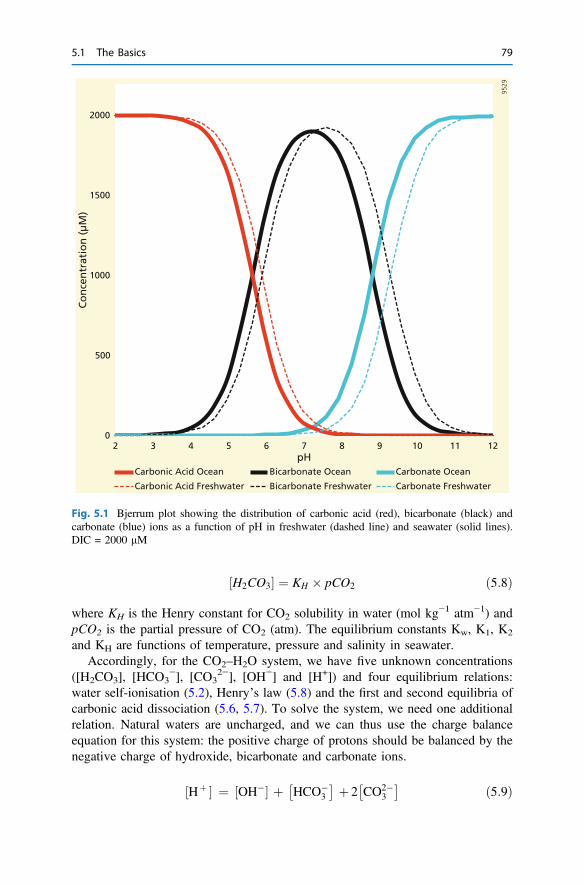
H2CO3½ � ¼ KH � pCO2 ð5:8Þ

where KH is the Henry constant for CO2 solubility in water (mol kg−1 atm−1) andpCO2 is the partial pressure of CO2 (atm). The equilibrium constants Kw, K1, K2

and KH are functions of temperature, pressure and salinity in seawater.Accordingly, for the CO2–H2O system, we have five unknown concentrations

([H2CO3], [HCO3−], [CO3

2−], [OH−] and [H+]) and four equilibrium relations:water self-ionisation (5.2), Henry’s law (5.8) and the first and second equilibria ofcarbonic acid dissociation (5.6, 5.7). To solve the system, we need one additionalrelation. Natural waters are uncharged, and we can thus use the charge balanceequation for this system: the positive charge of protons should be balanced by thenegative charge of hydroxide, bicarbonate and carbonate ions.

0

500

1000

1500

2000

2 3 4 5 6 7 8 9 10 11 12

Co

nce

ntr

atio

n (

µM

)

pH

9529

Bicarbonate Ocean Carbonate OceanCarbonic Acid Ocean

Bicarbonate Freshwater Carbonate FreshwaterCarbonic Acid Freshwater

Fig. 5.1 Bjerrum plot showing the distribution of carbonic acid (red), bicarbonate (black) andcarbonate (blue) ions as a function of pH in freshwater (dashed line) and seawater (solid lines).DIC = 2000 lM

Hþ½ � ¼ OH�½ � þ HCO�3

� � þ 2 CO2�3

� � ð5:9Þ

5.1 The Basics 79

Note that the carbonate ion is counted twice in a charge balance because of itsdouble charge. Alternatively, one can define a proton balance equation, a massbalance for protons (Butler 1982):

Hþ½ � ¼ Hþ½ �H2O þ Hþ½ �H2CO3ð5:10aÞ

or its equivalent

Hþ½ � ¼ OH�½ � þ HCO�3

� �þ 2 CO2�3

� �; ð5:10bÞ

This proton conservation equation balances excess protons on the left-hand sidewith the recipe on the right-hand side. Proton mass balances are always relative to aproton reference level, e.g. Equation (5.10a, b) is relative to H2CO3 and in this case,it is identical to the charge balance. Mathematically, the system is now fully definedwith 5 unknown species linked via 5 equations. Moreover, the system remains fullydetermined if another component is added for which the total concentration andequilibrium distribution among species is known.

5.2 The Thermodynamic Basis

So far, we have ignored non-ideal behaviour of gases, liquids and solutes that havean impact on equilibria. Although the name equilibrium constant suggests that it is aconstant, it is in fact not, because of its dependence on temperature, pressure andthe composition of the solution. This dependence relates to the effect of tempera-ture, pressure and mixture composition on the Gibbs Free energy. Formally, atequilibrium, the change in Gibbs free energy DGreact (J mol−1) is related to thethermodynamic equilibrium constant (Kx

therm) via DGreact ¼ �RT lnKthermx , where T

is in Kelvin and R is the universal gas constant (8.314 J mol−1 K−1).There are two generic pathways towards obtaining equilibrium constants for

complex natural solutions. The first approach involves calculating thermodynamicconstants from the well-documented and tabulated standard Gibbs free energies offormation and correcting these for temperature and pressure of the system. Thethermodynamic equilibrium constant is then expressed in activities of the moleculesinvolved, rather than concentrations. For example, equilibrium relation (5.3) for thethermodynamic K1

therm should formally be written as:

Ktherm1 ¼ HCO�

3

� �Hþf g

H2CO3f g

where the {} indicate that activities, rather than concentrations [] are used. Con-centrations and activities are linked via activity coefficients (c), which account forboth electrostatic interactions, as well as formation of ion-pairs among the variousions in solution:


Ktherm1 ¼ HCO�

3

� �H þf g

H2CO3f g ¼ HCO�3

� �H þ½ �

H2CO3½ � �cHCO�

3cH þ

cH2CO3

These activity coefficients are usually calculated using the Pitzer model (Millero2007) that can be applied to highly complex media, such as brines.

The alternative way of estimating equilibrium constants, used by most chemicaloceanographers and marine biogeochemists, is to experimentally determine stoi-chiometric constants as a function of temperature, pressure and salinity and rep-resent this dependency by a polynomial function. The underlying idea is that therelative composition of seawater is rather constant, that the reaction as such doesnot change the composition of seawater and that direct measurements in seawaterprovide more accurate results than using thermodynamic data with activity coeffi-cient corrections:

K�1; T ;S;Pð Þ ¼

HCO�3

� �H þ½ �

H2CO3½ �

where the * superscripts indicates that it is a stoichiometric quantity, rather thanthermodynamic constant and the subscripts T, S and P stand for temperature,salinity and pressure. The temperature, salinity and pressure dependence of stoi-chiometric constants result in rather complex and cumbersome expressions(Table 5.1), but there are many computer programs available to facilitate theirdetermination.

Figure 5.2 shows the stoichiometric constant expressed as pK1* as a function oftemperature and salinity. pK1* values decrease with increasing temperature andsalinity, or in other words, carbonic acid is more dissociated with increasing tem-perature or salinity. The ratio of the stoichiometric equilibrium constant (K1*) atsalinity 35 to the thermodynamic equilibrium constant (K1

therm) in pure water isabout 4.4–5. This salinity effect has consequences for the speciation of dissolvedinorganic carbon in seawater (Fig. 5.1). Similar dependencies apply to other stoi-chiometric constants. Moreover, this stoichiometric approach can also be used toaccurately quantify the solubility of minerals in seawater and will be used from nowon (while dropping the * superscript).

The solubility of gases, including CO2, is also a function of temperature, salinityand pressure (increasing salinity and temperature lower the solubility of gases).Thermodynamically, the fugacity of carbon dioxide is linked via the Henry constantto dissolved carbon dioxide: H2CO3½ � ¼ KH � fCO2. The fugacity is not exactly thesame as the partial pressure, the product of CO2 mol fraction (x0CO2

) times total gaspressure, as presented above (in Eq. 5.8). Because most readers are more familiarwith the pCO2, than fCO2, we will use the former notation, noting that they aredifferent.

5.2 The Thermodynamic Basis 81

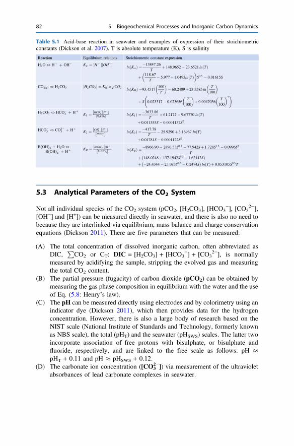
5.3 Analytical Parameters of the CO2 System

Not all individual species of the CO2 system (pCO2, [H2CO3], [HCO3−], [CO3

2−],[OH−] and [H+]) can be measured directly in seawater, and there is also no need tobecause they are interlinked via equilibrium, mass balance and charge conservationequations (Dickson 2011). There are five parameters that can be measured:

(A) The total concentration of dissolved inorganic carbon, often abbreviated asDIC,

PCO2 or CT: DIC = [H2CO3] + [HCO3

−] + [CO32−], is normally

measured by acidifying the sample, stripping the evolved gas and measuringthe total CO2 content.

(B) The partial pressure (fugacity) of carbon dioxide (pCO2) can be obtained bymeasuring the gas phase composition in equilibrium with the water and the useof Eq. (5.8: Henry’s law).

(C) The pH can be measured directly using electrodes and by colorimetry using anindicator dye (Dickson 2011), which then provides data for the hydrogenconcentration. However, there is also a large body of research based on theNIST scale (National Institute of Standards and Technology, formerly knownas NBS scale), the total (pHT) and the seawater (pHSWS) scales. The latter twoincorporate association of free protons with bisulphate, or bisulphate andfluoride, respectively, and are linked to the free scale as follows: pH �pHT + 0.11 and pH � pHSWS + 0.12.

(D) The carbonate ion concentration ([CO32−]) via measurement of the ultraviolet

absorbances of lead carbonate complexes in seawater.

Table 5.1 Acid-base reaction in seawater and examples of expression of their stoichiometricconstants (Dickson et al. 2007). T is absolute temperature (K), S is salinity

Reaction Equilibrium relations Stoichiometric constant expression

H2O , Hþ þ OH� Kw ¼ H þ½ � OH�½ �ln Kwð Þ ¼�13847:26

Tþ 148:9652� 23:6521 ln Tð Þ

þ 118:67T

� 5:977þ 1:0495ln Tð Þ� �

S0:5 � 0:01615S

CO2ðgÞ , H2CO3 H2CO3½ � ¼ KH � pCO2 ln KHð Þ ¼93:4517100T

� �� 60:2409þ 23:3585 ln

T

100

� �

þ S 0:023517� 0:023656T

100

� �þ 0:0047036

T

100

� �2 !

H2CO3 , HCO�3 þ Hþ

K1 ¼ HCO�3½ � Hþ½ �

H2CO3½ � ln K1ð Þ ¼�3633:86T

þ 61:2172� 9:67770 ln Tð Þþ 0:011555S� 0:0001152S2

HCO�3 , CO2�

3 þ HþK2 ¼ CO2�

3½ � H þ½ �HCO�

3½ � ln K2ð Þ ¼�417:78T

� 25:9290þ 3:16967 ln Tð Þþ 0:01781S� 0:0001122S2

B OHð Þ3 þ H2O ,B OHð Þ�4 þ Hþ KB ¼ B OHð Þ�4½ � Hþ½ �

B OHð Þ3½ � ln KBð Þ ¼�8966:90� 2890:53S0:5 � 77:942Sþ 1:728S1:5 � 0:0996S2

Tþ 148:0248þ 137:1942S0:5 þ 1:62142S�

þ �24:4344� 25:085S0:5 � 0:2474S�

ln Tð Þþ 0:053105S0:5T


(E) The total or titration alkalinity (TA), which can be seen as the excess of protonacceptors over donors of a solution and is normally derived from an acidi-metric titration. The total alkalinity of a solution is relatively easy to measure,and which has the pleasant characteristic that it behaves conservatively as twowaters are mixed or if temperature or pressure changes, similar to DIC.A formal definition and detailed treatment follow below.

Let us revisit the simple CO2–H2O system from above with five species([H2CO3], [HCO3

−], [CO32−], [OH−] and [H+]). Titration of this system with a

strong acid results in a decrease in pH and transformation of carbonate to bicar-bonate and bicarbonate to carbonic acid. Each bicarbonate ion can accept oneproton, each carbonate ion consumes two protons before it is transformed intocarbonic acid, and carbonic acid cannot accept protons. For this system, we candefine H2CO3 as our reference (zero level of protons). Similarly, the hydroxide ionsin solution will accept one proton, while any proton available just adds to the finalproton concentration at the end of a titration. TA was formally defined by Dickson(1981) as the excess of proton acceptors ([HCO3

−] + 2 [CO32−] + [OH−]) over

proton donors [H+] of the initial solution:

TA ¼ HCO�3

� � þ 2 CO2�3

� � þ OH� �� ½Hþ½ � ð5:11Þ

5.4

5.6

5.8

6

6.2

6.4

6.6

6.8

0 5 10 15 20 25 30 35

pK

val

ue

Temperature (°C)

9529

0

5

15

25

35

Fig. 5.2 The dependence of pK1 on the temperature and salinity of water

5.3 Analytical Parameters of the CO2 System 83

The reader might have noted that this TA definition has much similarity to thecharge balance and proton balance Eqs. (5.9), (5.10a, b) for this simple CO2–H2Osystem. If fact by re-arranging the charge balance (5.9) we obtain the charge balancealkalinity or excess negative charge (ENC):

ENC ¼ HCO�3

� � þ 2 CO2�3

� � þ OH� �� ½Hþ½ � ð5:12Þ

and we see that this excess negative charge is equivalent to the titration alkalinityfor this system. This excess negative charge introduced by Soetaert et al. (2007) isalso known as the explicit conservative equation of total alkalinity (Zeebe andWolf-Gladrow 2001; Wolf-Gladrow et al. 2007).

Although seawater is a much more complex system, because it contains manypotential proton acceptors and donors, such as borate, phosphate and silicate spe-cies, the same approach can be used. Dickson (1981) formally defined total alka-linity of filtered seawater by the excess of proton acceptors over proton donors withrespect to the proton condition at pH 4.5 (Dickson 1981), which then leads to theexpression:

TA ¼ HCO�3

� � þ 2 CO2�3

� � þ B OHð Þ�4� � þ OH�½ � þ HPO2�

4

� � þ 2 PO3�4

� � þ H3SiO�4

� �þ 2 H2SiO

2�4

� � þ NH3½ � þ HS�½ � þ 2 S2�� Hþ½ � � HF½ � � ½HSO�

4 ��2½H2SO4� � ½H3PO4� � ½HNO2� � ½HNO3�

ð5:13Þ

Following Wolf-Gladrow et al. (2007) and Soetaert et al. (2007), some additionalproton acceptors (H2SiO4

2−, S2−) and proton donors (HNO2, HNO3, H2SO4) havebeen added to the original definition of Dickson (1981). Most of these additionalterms are close to zero in oxic seawater. Moreover, TA in marine waters is dom-inated by the carbonate species and simpler relations than (5.13) are often used. Thecarbonate alkalinity (CA) is defined as the alkalinity contribution of bicarbonateand carbonate species:

CA ¼ HCO�3

� � þ 2 CO2�3

� � ð5:14Þ

and usually accounts for >95% of the alkalinity, with borate contributinganother *3–4%. While the presence of these additional species hardly impactsmeasurement of TA by titration, it will affect the use of TA in calculations to obtainthe sought-after distribution of bicarbonate and carbonate concentrations.

The excess negative charge concept, as introduced earlier (5.12) can also beapplied to seawater (Soetaert et al. 2007; Wolf-Gladrow et al. 2007):


ENC ¼ HCO�3

� � þ 2 CO2�3

� � þ B OHð Þ�4� � þ OH�½ � þ H2PO

�4

� � þ 2 HPO2�4

� � þ 3 PO3�4

� � þ H3SiO�4

� �þ 2 H2SiO

2�4

� � þ NO�3

� � þ NO�2

� � þ F�½ � þ HS�½ � þ 2 S2�� þ HSO�

4

� � þ 2 SO2�4

� �� Hþ½ � � NHþ4

� �:

ð5:15Þ

ENC and TA are related via:

TA ¼ ENC þX

NH4 �X

NO3 �X

NO2 �X

PO4 � 2X

SO4 �X

F

ð5:16Þ

where the variousP

-terms refer to total concentration of the respective acid-basepairs (e.g.

PNH4 = [NH4

+] + [NH3]). This difference between TA and ENC iscaused by components for which the species used as zero proton levels are charged.In other words, DIC and

PB(OH)3 do not appear because they are uncharged at

their zero proton level. This distinction between TA measured by titration (sensuDickson) and ENC (charge balance alkalinity) is needed to understand the impact ofbiogeochemical processes on pH or pCO2, in particular those involvingion-exchange or nutrient uptake (Zeebe and Wolf-Gladrow 2001; Soetaert et al.2007; Wolf-Gladrow et al. 2007). For instance, nitrate or ammonium uptake byphytoplankton has a distinct effect on TA (decrease and increase, respectively;Brewer and Goldman 1976; Goldman and Brewer 1980) that cannot be inferredfrom the Dickson definition of TA (5.13), but is clear from Eqs. 5.15 and 5.16. Theconcept of potential alkalinity (Brewer et al. 1975) and its derivatives, such as TA*,are special cases of the ENC concept. The need to correct for nutrient cycling whenusing the alkalinity anomaly technique to quantify calcification is also made explicitwhen using Eq. 5.16.

5.4 Buffering

Natural waters, in particular seawater, contain multiple weak acids and their con-jugate bases. Any addition or removal of an acid or base results in re-adjustment ofthe equilibrium distribution of acids and conjugated bases, with the consequencethat the disturbance is attenuated (the principle of le Chatelier). Buffering caninvolve only dissolved components (homogenous) or also solid phases (heteroge-neous). Heterogenous buffering in the ocean is called ocean carbonate compensa-tion (Box 5.2). Homogenous buffering of waters is most often quantified by thebuffering value (B), which is formally defined as the concentration of acid or baseto be added to influence pH (Van Slycke 1922; Urbanksy and Schock 2000):

B ¼ dCb

dpH¼ � dCa

dpH; ð5:17Þ

5.3 Analytical Parameters of the CO2 System 85

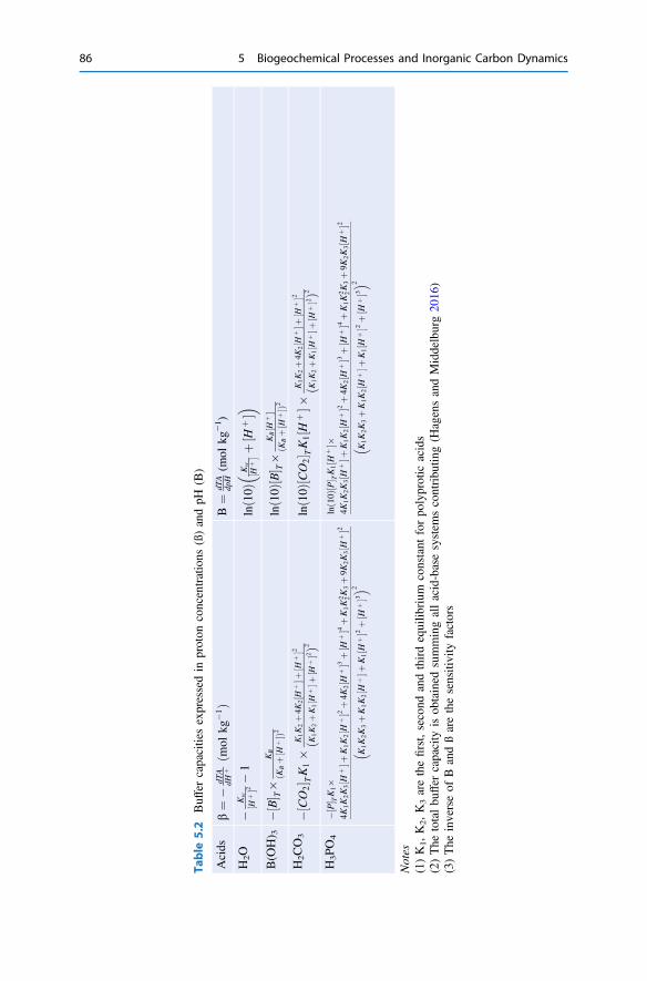
Table

5.2

Buffercapacitiesexpressedin

proton

concentrations

(ß)andpH

(B)

Acids

b¼

�dT

AdH

þðm

olkg

�1Þ

B¼

dTA

dpH(m

olkg

−1 )

H2O

�Kw

Hþ

½�2�1

ln10ð

ÞKw

Hþ

½�þ

Hþ

½�

�

B(O

H) 3

�B½� T�

KB

KBþ

Hþ

½�

ðÞ2

ln10ð

ÞB½� T�

KBH

þ½

�KBþ

Hþ

½�

ðÞ2

H2C

O3

�CO

2½

� TK1�

K1K2þ4K

2H

þ½

�þH

þ½

�2K1K2þK1H

þ½

�þH

þ½

�2ð

Þ2ln

10ðÞC

O2

½� TK

1H

þ½

��K1K2þ4K

2H

þ½

�þH

þ½

�2K1K2þK1H

þ½

�þH

þ½

�2ð

Þ2

H3PO4

�P½� TK

1�

4K1K2K3H

þ½

�þK1K2H

þ½

�2 þ4K

2H

þ½

�3 þH

þ½

�4 þK1K

2 2K3þ9K

2K3H

þ½

�2

K1K2K3þK1K2H

þ½

�þK1H

þ½

�2 þH

þ½

�3

� 2ln

10ðÞP½

� TK1H

þ½

��4K

1K2K3H

þ½

�þK1K2H

þ½

�2 þ4K

2H

þ½

�3 þH

þ½

�4 þK1K

2 2K3þ9K

2K3H

þ½

�2

K1K2K3þK1K2H

þ½

�þK1H

þ½

�2 þH

þ½

�3

� 2

Notes

(1)K1,K2,K3arethefirst,second

andthirdequilib

rium

constant

forpo

lyprotic

acids

(2)The

totalbu

ffer

capacity

isob

tained

summingallacid-basesystem

scontribu

ting(H

agensandMiddelburg20

16)

(3)The

inverseof

Bandßarethesensitivity

factors


where Cb and Ca are the concentration of added base and acid, respectively. Theterm buffer value as used here is identical to the terms buffer capacity, intensity andindex in use by analytical chemists, geochemists and engineers. Buffer values arealways positive because solutions resist changes according to the le Chatelierprinciple; consequently, a minus is needed when considering acid addition. Thebuffer value is a continuous non-linear function, as it is the inverse of the slope ofthe titration curve, i.e. a derivative (Stumm and Morgan 1996). The buffering valueof seawater is expressed using the total alkalinity:

B ¼ dTA

dpH: ð5:18Þ

For notational simplicity, we present buffer value as a derivative, while it is a partialderivative because all other concentrations are kept constant when determining thisbuffer value by titration (Hagens and Middelburg 2016). Van Slycke’s originaldefinition of buffer value was in pH, but in seawater it is instructive to expressbuffering value in terms of proton concentration (b):

b ¼ � dTA

dH þ : ð5:19Þ

Buffer values B and b are linked via B = –ln(10)* H+* b. Table 5.2 gives the

relevant equations for B (in pH) and b (in proton concentrations).Total alkalinity includes multiple acid-base systems, and the overall buffering

value can be obtained by summing the contributions of all the acid-base systemsinvolved (Urbanksy and Schock 2000). The buffer value of seawater is mainlydetermined by the borate and carbonate contributions, and we therefore limited ourcalculations to these (and of course the contribution of water). The buffer value ofseawater (S = 35, T = 15 °C, DIC = 2000 µM) is a function of pH and has twodistinct maxima at pH 6 and 8.9, near the pK1 and pK2 of the carbonate system inseawater and a minimum at pH 7.4 (approximately midway between these maxima;Fig. 5.3). Within the pH range of 7.5–8.5 the buffer value increases with pH andcan be approximated by the relation:

B ffi ln 10ð ÞK2DIC

H þ ; ð5:20Þ

showing that the buffer value of seawater in its normal range primarily depends onthe DIC concentration, the pH and pK2 value. Borate contributes about 15–22% toseawater buffering in this range.

5.4 Buffering 87

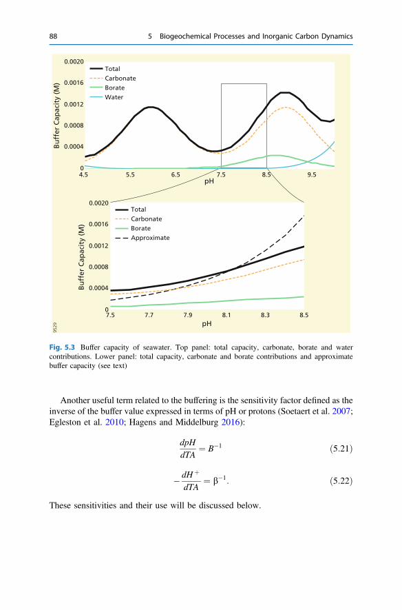
Another useful term related to the buffering is the sensitivity factor defined as theinverse of the buffer value expressed in terms of pH or protons (Soetaert et al. 2007;Egleston et al. 2010; Hagens and Middelburg 2016):

dpH

dTA¼ B�1 ð5:21Þ

� dH þ

dTA¼ b�1: ð5:22Þ

These sensitivities and their use will be discussed below.

0

0.0004

0.0008

0.0012

0.0016

0.0020

0

0.0004

0.0008

0.0012

0.0016

0.0020

4.5 5.5 6.5 7.5 8.5 9.5

7.5 7.7 7.9 8.1 8.3 8.5

Bu

ffer

Cap

acit

y (M

)

Bu

ffer

Cap

acit

y (M

)

pH

pH

9529

Total

Carbonate

Borate

Water

Total

Carbonate

Borate

Approximate

Fig. 5.3 Buffer capacity of seawater. Top panel: total capacity, carbonate, borate and watercontributions. Lower panel: total capacity, carbonate and borate contributions and approximatebuffer capacity (see text)


5.5 Carbonate Mineral Equilibria

In the above section, we only considered homogenous buffering, i.e. there-equilibration among dissolved species. In natural systems, solid phases alsocontribute to buffering via dissolution and precipitation, and we call this hetero-geneous buffering. Carbonate minerals play a dominant role in heterogeneousbuffering because of their omnipresence, high solubility and high reactivity.

The precipitation and dissolution of calcium carbonate is represented by thereaction:

Ca2þ þ CO2�3 , CaCO3 ð5:23Þ

for which we can write the equilibrium relation:

Ksp ¼ Ca2þ� �

CO2�3

� � ð5:24Þ

where Ksp is the stoichiometric solubility product for calcium carbonate, which is afunction of temperature, salinity, pressure and the calcium carbonate mineral. Thesolubility product is used to calculate the saturation state of seawater (X) withrespect to the calcium carbonate mineral:

X ¼ Ca2þ½ � CO2�3

� �Ksp

: ð5:25Þ

If X = 1, then the solution is in equilibrium with that mineral, if X > 1, then thesolution is supersaturated with respect to that mineral and if X < 1, then thesolution is undersaturated with respect to that mineral. Undersaturation andsupersaturation promote dissolution and precipitation, respectively.

The two dominant calcium carbonate minerals in the ocean are calcite andaragonite, which differ in crystal structure, mineralogical properties (e.g. density)and solubility (Morse et al. 2007). The thermodynamic solubility products of calcite(pK = 8.48) and aragonite (pK = 8.30) differ by a factor 1.5, while their stoi-chiometric solubility products at salinity 35 and T = 25 °C are more than twoorders of magnitude higher (pK = 6.36 and 6.18, respectively). The crystal struc-ture of carbonates has consequences for the incorporation of other ions, with largercations (e.g., Sr2+, Ba2+) preferably incorporated in the orthorhombic aragonitestructure and smaller cations (e.g., Mg2+, Mn2+) fitting better in the hexagonalcalcite structure. Dissolved magnesium concentrations in seawater are rather high(>5 times Ca2+) and Mg incorporation is therefore substantial (up to *25% forbiogenic carbonates), with large consequences for solubility. The solubility ofMg-calcite with about 2% Mg is lower than that of pure calcite, while calcites withabout 12–15% Mg substitution are five times more soluble than aragonite(Arvidson and Morse 2014).

5.6 Dissolved Inorganic Carbon Systematics 89

5.6 Dissolved Inorganic Carbon Systematics

The conservative properties TA and DIC are often used as master variables toanalyse the impact of environmental change on the marine CO2 system, because thedistribution of the species carbonic acid, bicarbonate and carbonate, and pCO2 andpH depend on temperature and salinity. Figure 5.4 shows the temperature depen-dence of pH, pCO2, bicarbonate and carbonate ion concentrations for seawater(TA = 2300 µM, DIC = 2000 µM). Increasing temperatures will cause an almostlinear decrease in pH with a slope of –0.0155 pH/°C, while it will cause anexponential increase in pCO2 values. Bicarbonate and carbonate ion concentrationswill decrease and increase with increasing temperatures (slopes of about −0.55and +0.42 lM/0C, respectively).

There are also distinct dependencies with salinity (Fig. 5.4), but these only includethe impact of salinity on stoichiometric equilibrium constants, not the larger effect ofsalinity on total alkalinity via charge balance. Increasing salinity results in a decline inpH and carbonate ion concentration and an increase in bicarbonate and pCO2.

Relations among TA, DIC, pCO2 and pH are often presented graphically in theform of TA versus DIC plots with isolines for pH or pCO2 (Fig. 5.5) for seawater(T = 15, S = 35). The addition or removal of TA or DIC or any of its constituentson such a plot is a vector property (Deffeyes 1965). For instance, CO2 addition willincrease DIC concentration, but not affect TA and thus result in a horizontal vectorpointing to the right; pCO2 of the water will increase and the pH will decline.Addition of protons will decrease TA, but not impact DIC; the downward headingvertical vector indicates that pH will decline and pCO2 will increase. The additionof HCO3

− will impact both DIC and TA by one unit; the vector will have a slope ofone and both pH and pCO2 will slightly increase. The addition of CO3

2− willincrease DIC by one unit and TA by two units, and the resulting vector indicates alowering in pCO2 and increase in pH.

5.7 The Impact of Biogeochemical Processes

Most biological and physical exchange processes occur on longer time scales thanthe chemical equilibrium reactions, and any addition or removal of a compound dueto biology and physics thus causes re-equilibrations following the le Chatelierprinciple; i.e. buffering occurs. The impact of biogeochemical processes on thedissolved inorganic carbon system can be analysed (graphically or numerically)using their impact on DIC and TA.

Gas exchange. Invasion of CO2 from the atmosphere into seawater causes anincrease in DIC, but does not change TA, with the consequence that pCO2 increasesand pH declines. The reverse process, an efflux of CO2 from seawater to theatmosphere, results in pCO2 decline and pH increase (Fig. 5.6). These CO2

exchange processes may be initiated either by changing atmospheric mixing ratiosof CO2 or by cooling or warming of seawater.


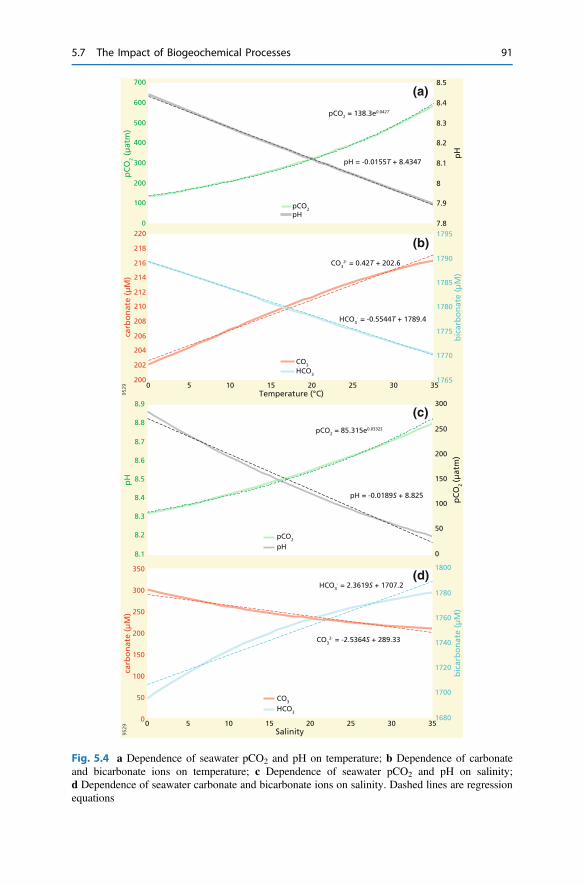
0

100

200

300

400

500

600

700

200

202

204

206

208

210

212

214

216

218

2207.8

7.9

8

8.1

8.2

8.3

8.4

8.5

1765

1770

1775

1780

1785

1790

1795

0 5 10 15 20 25 30 35

pH

pC

O2

(µat

m)

bic

arb

on

ate

(µM

)

carb

on

ate

(µM

)

Temperature (°C)9529

pCO2 = 138.3e0.042T

pH = -0.0155T + 8.4347

CO32- = 0.42T + 202.6

HCO3- = -0.5544T + 1789.4

CO3

HCO3

pCO2pH

1680

1700

1720

1740

1760

1780

1800

8.1

8.2

8.3

8.4

8.5

8.6

8.7

8.8

8.9

0

50

100

150

200

250

300

0

50

100

150

200

250

300

350

0 5 10 15 20 25 30 35

pC

O2 (µ

atm

)

pH

bic

arb

on

ate

(µM

)

carb

on

ate

(µM

)

Salinity9529

pH = -0.0189S + 8.825

pCO2 = 85.315e0.0332S

CO32- = -2.5364S + 289.33

HCO3- = 2.3619S + 1707.2

CO3

HCO3

pHpCO2

(a)

(b)

(c)

(d)

Fig. 5.4 a Dependence of seawater pCO2 and pH on temperature; b Dependence of carbonateand bicarbonate ions on temperature; c Dependence of seawater pCO2 and pH on salinity;d Dependence of seawater carbonate and bicarbonate ions on salinity. Dashed lines are regressionequations

5.7 The Impact of Biogeochemical Processes 91

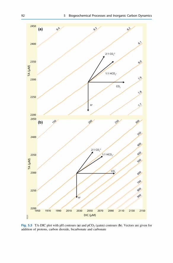
2200

2250

2300

2350

2400

2450

2200

2250

2300

2350

2400

2450

1950 1970 1990 2010 2030 2050 2070 2090 2110 2130 2150

TA (

µM

)TA

(µ

M)

DIC (µM)

9529

CO2

H+

1:1 HCO3-

2:1 CO32-

CO2

H+

1:1 HCO3-

2:1 CO32-

7.7

7.8

7.9

8.0

8.1

8.28.38.4

150200

250300

350

400

450

500

600

700

800

900

(a)

(b)

Fig. 5.5 TA-DIC plot with pH contours (a) and pCO2 (µatm) contours (b). Vectors are given foraddition of protons, carbon dioxide, bicarbonate and carbonate


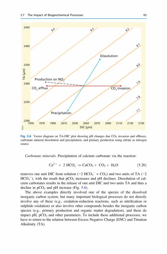
Carbonate minerals. Precipitation of calcium carbonate via the reaction:

Ca2þ þ 2 HCO�3 ) CaCO3 þ CO2 þ H2O ð5:26Þ

removes one unit DIC from solution (−2 HCO3− + CO2) and two units of TA (−2

HCO3−), with the result that pCO2 increases and pH declines. Dissolution of cal-

cium carbonates results in the release of one unit DIC and two units TA and thus adecline in pCO2 and pH increase (Fig. 5.6).

The above examples directly involved one of the species of the dissolvedinorganic carbon system, but many important biological processes do not directlyinvolve any of these (e.g., oxidation-reduction reactions, such as nitrification orsulphide oxidation) or also involve other compounds besides the inorganic carbonspecies (e.g., primary production and organic matter degradation), and these doimpact pH, pCO2 and other parameters. To include these additional processes, wehave to return to the relation between Excess Negative Charge (ENC) and TitrationAlkalinity (TA).

2200

2250

2300

2350

2400

2450

1950 1970 1990 2010 2030 2050 2070 2090 2110 2130 2150

TA (

µm

)

DIC (µm)

9529

CO2 invasion

Dissolution

CO2 efflux

Precipitation

Production on NO3-

7.7

7.8

7.9

8.0

8.1

8.28.38.4

Fig. 5.6 Vector diagram on TA-DIC plot showing pH changes due CO2 invasion and effluxes,carbonate mineral dissolution and precipitation, and primary production using nitrate as nitrogensource


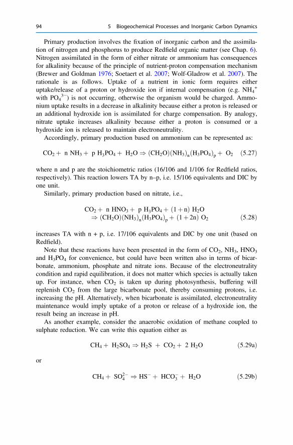
Primary production involves the fixation of inorganic carbon and the assimila-tion of nitrogen and phosphorus to produce Redfield organic matter (see Chap. 6).Nitrogen assimilated in the form of either nitrate or ammonium has consequencesfor alkalinity because of the principle of nutrient-proton compensation mechanism(Brewer and Goldman 1976; Soetaert et al. 2007; Wolf-Gladrow et al. 2007). Therationale is as follows. Uptake of a nutrient in ionic form requires eitheruptake/release of a proton or hydroxide ion if internal compensation (e.g. NH4

+

with PO43−) is not occurring, otherwise the organism would be charged. Ammo-

nium uptake results in a decrease in alkalinity because either a proton is released oran additional hydroxide ion is assimilated for charge compensation. By analogy,nitrate uptake increases alkalinity because either a proton is consumed or ahydroxide ion is released to maintain electroneutrality.

Accordingly, primary production based on ammonium can be represented as:

CO2 þ n NH3 þ p H3PO4 þ H2O ) CH2Oð Þ NH3ð Þn H3PO4ð Þp þ O2 ð5:27Þ

where n and p are the stoichiometric ratios (16/106 and 1/106 for Redfield ratios,respectively). This reaction lowers TA by n–p, i.e. 15/106 equivalents and DIC byone unit.

Similarly, primary production based on nitrate, i.e.,

CO2 þ n HNO3 þ p H3PO4 þ 1þ nð Þ H2O) CH2Oð Þ NH3ð Þn H3PO4ð Þp þ 1þ 2nð Þ O2 ð5:28Þ

increases TA with n + p, i.e. 17/106 equivalents and DIC by one unit (based onRedfield).

Note that these reactions have been presented in the form of CO2, NH3, HNO3

and H3PO4 for convenience, but could have been written also in terms of bicar-bonate, ammonium, phosphate and nitrate ions. Because of the electroneutralitycondition and rapid equilibration, it does not matter which species is actually takenup. For instance, when CO2 is taken up during photosynthesis, buffering willreplenish CO2 from the large bicarbonate pool, thereby consuming protons, i.e.increasing the pH. Alternatively, when bicarbonate is assimilated, electroneutralitymaintenance would imply uptake of a proton or release of a hydroxide ion, theresult being an increase in pH.

As another example, consider the anaerobic oxidation of methane coupled tosulphate reduction. We can write this equation either as

CH4 þ H2SO4 ) H2S þ CO2 þ 2 H2O ð5:29aÞ

or

CH4 þ SO2�4 ) HS� þ HCO�

3 þ H2O ð5:29bÞ


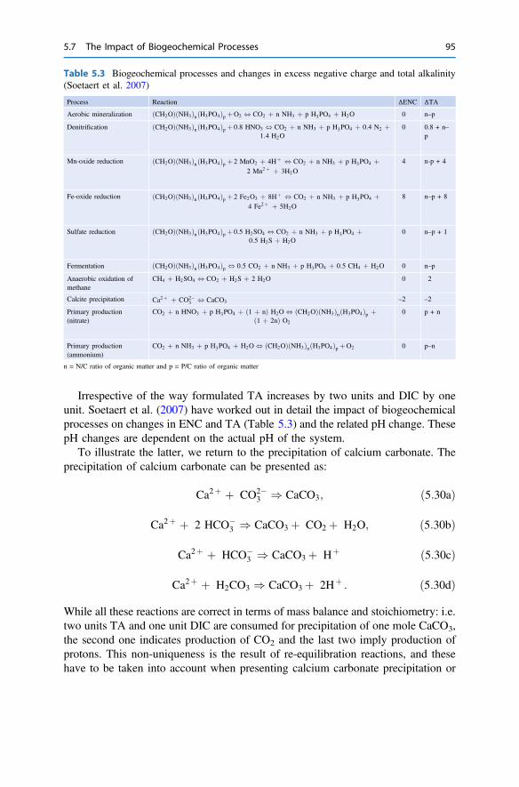
Irrespective of the way formulated TA increases by two units and DIC by oneunit. Soetaert et al. (2007) have worked out in detail the impact of biogeochemicalprocesses on changes in ENC and TA (Table 5.3) and the related pH change. ThesepH changes are dependent on the actual pH of the system.

To illustrate the latter, we return to the precipitation of calcium carbonate. Theprecipitation of calcium carbonate can be presented as:

Ca2þ þ CO2�3 ) CaCO3; ð5:30aÞ

Ca2þ þ 2 HCO�3 ) CaCO3 þ CO2 þ H2O; ð5:30bÞ

Ca2þ þ HCO�3 ) CaCO3 þ Hþ ð5:30cÞ

Ca2þ þ H2CO3 ) CaCO3 þ 2Hþ : ð5:30dÞ

While all these reactions are correct in terms of mass balance and stoichiometry: i.e.two units TA and one unit DIC are consumed for precipitation of one mole CaCO3,the second one indicates production of CO2 and the last two imply production ofprotons. This non-uniqueness is the result of re-equilibration reactions, and thesehave to be taken into account when presenting calcium carbonate precipitation or

Table 5.3 Biogeochemical processes and changes in excess negative charge and total alkalinity(Soetaert et al. 2007)

Process Reaction ΔENC ΔTA

Aerobic mineralization CH2Oð ÞðNH3ÞnðH3PO4Þp þO2 , CO2 þ n NH3 þ p H3PO4 þ H2O 0 n–p

Denitrification CH2Oð ÞðNH3ÞnðH3PO4Þp þ 0:8 HNO3 , CO2 þ n NH3 þ p H3PO4 þ 0:4 N2 þ1:4 H2O

0 0.8 + n–p

Mn-oxide reduction CH2Oð ÞðNH3ÞnðH3PO4Þp þ 2 MnO2 þ 4Hþ , CO2 þ n NH3 þ p H3PO4 þ2 Mn2þ þ 3H2O

4 n-p + 4

Fe-oxide reduction CH2Oð ÞðNH3ÞnðH3PO4Þp þ 2 Fe2O3 þ 8Hþ , CO2 þ n NH3 þ p H3PO4 þ4 Fe2þ þ 5H2O

8 n–p + 8

Sulfate reduction CH2Oð ÞðNH3ÞnðH3PO4Þp þ 0:5 H2SO4 , CO2 þ n NH3 þ p H3PO4 þ0:5 H2S þ H2O

0 n–p + 1

Fermentation CH2Oð ÞðNH3ÞnðH3PO4Þp , 0:5 CO2 þ n NH3 þ p H3PO4 þ 0:5 CH4 þ H2O 0 n–p

Anaerobic oxidation ofmethane

CH4 þ H2SO4 , CO2 þ H2S þ 2 H2O 0 2

Calcite precipitation Ca2þ þ CO2�3 , CaCO3 –2 –2

Primary production(nitrate)

CO2 þ n HNO3 þ p H3PO4 þ ð1 þ nÞ H2O , CH2Oð ÞðNH3ÞnðH3PO4Þp þð1 þ 2nÞ O2

0 p + n

Primary production(ammonium)

CO2 þ n NH3 þ p H3PO4 þ H2O , CH2Oð ÞðNH3ÞnðH3PO4Þp þO2 0 p–n

n = N/C ratio of organic matter and p = P/C ratio of organic matter


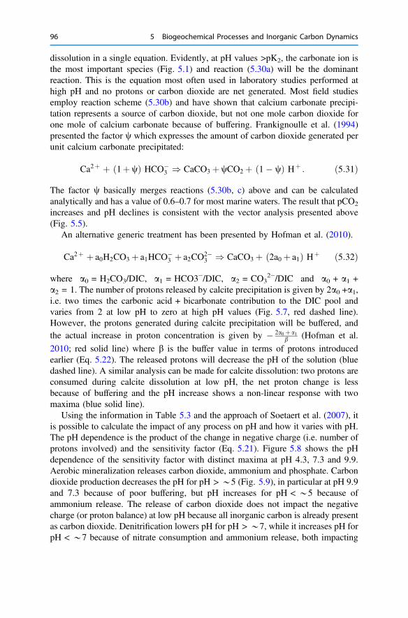
dissolution in a single equation. Evidently, at pH values >pK2, the carbonate ion isthe most important species (Fig. 5.1) and reaction (5.30a) will be the dominantreaction. This is the equation most often used in laboratory studies performed athigh pH and no protons or carbon dioxide are net generated. Most field studiesemploy reaction scheme (5.30b) and have shown that calcium carbonate precipi-tation represents a source of carbon dioxide, but not one mole carbon dioxide forone mole of calcium carbonate because of buffering. Frankignoulle et al. (1994)presented the factor w which expresses the amount of carbon dioxide generated perunit calcium carbonate precipitated:

Ca2þ þ ð1þwÞ HCO�3 ) CaCO3 þwCO2 þ ð1� wÞ Hþ : ð5:31Þ

The factor w basically merges reactions (5.30b, c) above and can be calculatedanalytically and has a value of 0.6–0.7 for most marine waters. The result that pCO2

increases and pH declines is consistent with the vector analysis presented above(Fig. 5.5).

An alternative generic treatment has been presented by Hofman et al. (2010).

Ca2þ þ a0H2CO3 þ a1HCO�3 þ a2CO

2�3 ) CaCO3 þ ð2a0 þ a1Þ Hþ ð5:32Þ

where a0 = H2CO3/DIC, a1 = HCO3−/DIC, a2 = CO32−/DIC and a0 + a1 +

a2 = 1. The number of protons released by calcite precipitation is given by 2a0 +a1,i.e. two times the carbonic acid + bicarbonate contribution to the DIC pool andvaries from 2 at low pH to zero at high pH values (Fig. 5.7, red dashed line).However, the protons generated during calcite precipitation will be buffered, andthe actual increase in proton concentration is given by � 2a0 þ a1

b (Hofman et al.2010; red solid line) where b is the buffer value in terms of protons introducedearlier (Eq. 5.22). The released protons will decrease the pH of the solution (bluedashed line). A similar analysis can be made for calcite dissolution: two protons areconsumed during calcite dissolution at low pH, the net proton change is lessbecause of buffering and the pH increase shows a non-linear response with twomaxima (blue solid line).

Using the information in Table 5.3 and the approach of Soetaert et al. (2007), itis possible to calculate the impact of any process on pH and how it varies with pH.The pH dependence is the product of the change in negative charge (i.e. number ofprotons involved) and the sensitivity factor (Eq. 5.21). Figure 5.8 shows the pHdependence of the sensitivity factor with distinct maxima at pH 4.3, 7.3 and 9.9.Aerobic mineralization releases carbon dioxide, ammonium and phosphate. Carbondioxide production decreases the pH for pH > *5 (Fig. 5.9), in particular at pH 9.9and 7.3 because of poor buffering, but pH increases for pH < *5 because ofammonium release. The release of carbon dioxide does not impact the negativecharge (or proton balance) at low pH because all inorganic carbon is already presentas carbon dioxide. Denitrification lowers pH for pH > *7, while it increases pH forpH < *7 because of nitrate consumption and ammonium release, both impacting


the negative excess charge and TA (Eq. 5.16), in particular at pH 4.3 because of thehigh sensitivity factor (Fig. 5.8). Manganese and iron oxide reduction alwaysincrease pH with the relative pH increase primarily depending on the sensitivityfactor (Fig. 5.9).

Box 5.1: Ocean acidificationAtmospheric carbon dioxide concentrations steadily increased during the lastcentury because of the use of carbon-based energy resources, changes in landuse, and lime production. Part of this additional carbon dioxide remains in theatmosphere, i.e. an airborne fraction of about 45%, and is the main driver ofglobal warming. The other part ends up in the ocean or terrestrial biosphere.The ocean uptake of anthropogenic carbon accounts for 25–30%, but thisservice to humankind comes at a price: acid-base equilibria in the ocean haveshifted. DIC and bicarbonate concentrations increased (carbonation), whilecarbonate ions and pH declined (ocean acidification). Ocean acidification, or

0

0.5

1

1.5

2

2.5

0

0.001

0.002

0.003

0.004

0.005

0.006

0.007

0.008

0.009

0.01

0 2 4 6 8 10 12 14

Pro

ton

ch

ang

e

pH

pH

ch

ang

e

9529

Protons after bufferingProtons

DissolutionPrecipitation

Fig. 5.7 Calcium carbonate precipitation/dissolution, proton and pH changes as function of pH.The number of proton generated per mole calcite formed/dissolved before buffering (red dashedline) and after buffering (red solid line). The decline in pH for precipitation of one lmole of calcite(dashed blue line) and increase in pH for dissolution of one lmole calcite (solid blue line). There isa break at the pH where calcite starts to dissolve or precipitate


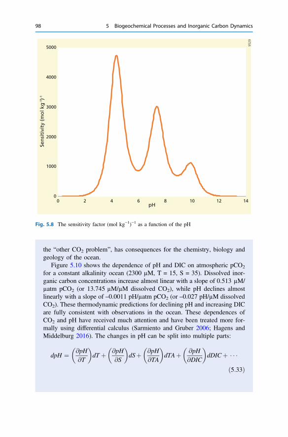
the “other CO2 problem”, has consequences for the chemistry, biology andgeology of the ocean.

Figure 5.10 shows the dependence of pH and DIC on atmospheric pCO2

for a constant alkalinity ocean (2300 µM, T = 15, S = 35). Dissolved inor-ganic carbon concentrations increase almost linear with a slope of 0.513 µM/µatm pCO2 (or 13.745 µM/µM dissolved CO2), while pH declines almostlinearly with a slope of –0.0011 pH/µatm pCO2 (or –0.027 pH/µM dissolvedCO2). These thermodynamic predictions for declining pH and increasing DICare fully consistent with observations in the ocean. These dependences ofCO2 and pH have received much attention and have been treated more for-mally using differential calculus (Sarmiento and Gruber 2006; Hagens andMiddelburg 2016). The changes in pH can be split into multiple parts:

dpH ¼ @pH

@T

� �dT þ @pH

@S

� �dSþ @pH

@TA

� �dTAþ @pH

@DIC

� �dDICþ � � �

ð5:33Þ

0

1000

2000

3000

4000

5000

0 2 4 6 8 10 12 14pH

Sen

siti

vity

(m

ol k

g-1)-1

9529

Fig. 5.8 The sensitivity factor (mol kg−1)−1 as a function of the pH


where @pH@x

�are partial derivatives, implying that these are, in principle, only

valid if the other variables are kept constant, and they can be considered as ameasure of the sensitivity of pH to a change in the respective environmental

variable. For instance, the first partial derivative, @pH@T

�has a value of

*–0.014 per degree (Hagens and Middelburg 2016), close to slope in

Fig. 5.10 (–0.015 per degree). The third one, @pH@TA

�, is the sensitivity factor

(Eq. 5.21) shown in Fig. 5.8.

0

1000

2000

3000

4000

5000

0

1000

2000

3000

4000

5000

0

0.01

0.02

0.03

0.04

0.05

-0.005

-0.004

-0.003

-0.002

-0.001

0

0.001

0.002

0.003

0.004

0.005

0 2 4 6 8 10 12 14

Sensitivity (m

ol kg

-1) -1Sen

sitivity (mo

l kg-1) -1

pH

ch

ang

ep

H c

han

ge

pH

9529

Iron Reduction

Manganese Reduction

Aerobic Mineralization

Denitrification

(a)

(b)

Fig. 5.9 a pH change due to iron-oxide and manganese oxide reduction as function of pH; b pHchange due to aerobic mineralization and denitrification as a function of pH. The sensitivity factor(Fig. 5.8) is shown as reference (grey)


Ocean acidification will lead to a decrease in buffer value (Fig. 5.3), andthis is one of the reasons why the ocean is projected to take up lessanthropogenic carbon in the future (besides changes in ocean physics andbiology). Consequently, the ocean carbon dioxide system will be more sen-sitive to changes, and diurnal and seasonal changes in pH are projected toincrease. Moreover, shifting chemical equilibria will have consequences forsound attenuation in the ocean.

7.95

8

8.05

8.1

8.15

8.2

7.95

8

8.05

8.1

8.15

8.2

2000

2020

2040

2060

2080

2100

2120

2140

2000

2020

2040

2060

2080

2100

2120

2140

270 320 370 420 470

8 10 12 14 16 18 20

pH

pH

DIC

(µ

M)

DIC

(µ

M)

pCO2 (µatm)

CO2 (µM)

pH = -0.001pCO2 + 8.45

DIC = 0.513pCO2 + 1873.9

pH = -0.027CO2 + 8.45

DIC = 13.745CO2 + 1874

pH TCO2

(a)

(b)

Fig. 5.10 pH and DIC dependence on pCO2 (µatm) (a) and dissolved CO2 (µM) (b). Regressionlines are shown as dashed lines


Many organisms, autotrophs as well as heterotrophs, will be impacted byeither the decline in pH and carbonate ions or the increase in dissolvedinorganic carbon. The latter, carbonation, might stimulate primary producers,which are carbon limited at the moment. Most calcifying organisms are likelygoing to suffer from the decrease in carbonate ion availability, but calcifi-cation is under biological control and sometimes completed inside theorganism, such that these responses are rather complex (Kroeker et al. 2013).

Box 5.2: Carbonate compensation dynamicsBuffering in the ocean not only occurs homogenously by re-arrangement ofacids and conjugated bases, but also heterogeneously by re-adjustment of thebalance between precipitation and dissolution of carbonate minerals. Whilehomogenous buffering is fast (instantaneous equilibria), heterogeneousbuffering has a larger capacity because of the large stock of carbonate min-erals stored in marine sediments. This heterogeneous buffering is calledcarbonate compensation and biology plays a major role.

Carbonate minerals are predominantly formed biologically in the modernocean, but there are a few exceptions, such as the formation of ooids intropical systems and authigenic calcite and dolomite formation in sediments.However, even in these cases, biology plays indirectly a major role bygoverning the chemical composition of the fluids they formed in (e.g. car-bonate formation induced by alkalinity production resulting from anaerobicoxidation of methane). Biological carbonate formation takes place in thewater column by autotrophs (e.g., coccoliths) and heterotrophs (pteropodsand foraminifera) and in the benthos by various organisms, autotrophs (e.g.coralline algae) and heterotrophs (e.g., corals, crustaceans, and molluscs).Biogenic carbonates can be aragonite, calcite or high-Mg calcites and com-binations thereof.

Following death of calcifiers in benthic systems, the biogenic carbonatecan either dissolve or accumulate at the seafloor and be buried. Carbonateproduced in the surface layer of the open ocean can dissolve in the watercolumn while particles settle, dissolve at the seafloor, or accumulate in sed-iments. Accumulation of biogenic carbonate is a prominent feature of oceansediments; some sediments consists almost entirely of biogenic carbonatedebris. Dissolution of carbonate is primarily driven by undersaturation, andorganisms contribute to dissolution in a number of ways. One, many biogenicminerals have organic layers and microbial degradation of these layersexposes new surfaces to undersaturated solutions. Two, boring organisms(sponges, fungi) weaken the structure and texture of biogenic carbonate andconsequently accelerate dissolution. Three, the metabolic activity of organ-isms has consequences for the saturation state of solution, e.g. carbon dioxide


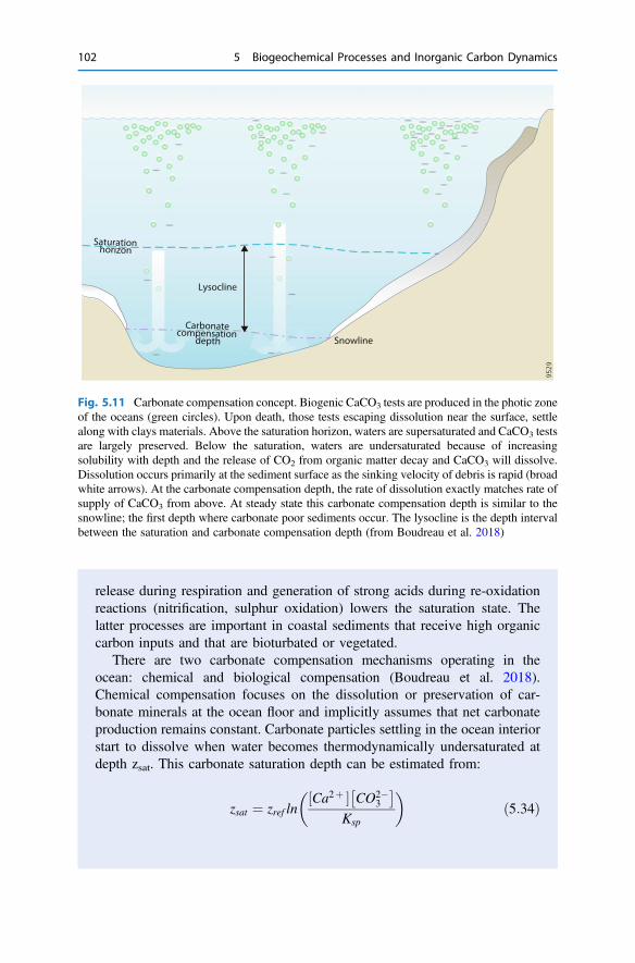
release during respiration and generation of strong acids during re-oxidationreactions (nitrification, sulphur oxidation) lowers the saturation state. Thelatter processes are important in coastal sediments that receive high organiccarbon inputs and that are bioturbated or vegetated.

There are two carbonate compensation mechanisms operating in theocean: chemical and biological compensation (Boudreau et al. 2018).Chemical compensation focuses on the dissolution or preservation of car-bonate minerals at the ocean floor and implicitly assumes that net carbonateproduction remains constant. Carbonate particles settling in the ocean interiorstart to dissolve when water becomes thermodynamically undersaturated atdepth zsat. This carbonate saturation depth can be estimated from:

zsat ¼ zref lnCa2þ½ � CO2�

3

� �Ksp

� �ð5:34Þ

9529

Fig. 5.11 Carbonate compensation concept. Biogenic CaCO3 tests are produced in the photic zoneof the oceans (green circles). Upon death, those tests escaping dissolution near the surface, settlealong with clays materials. Above the saturation horizon, waters are supersaturated and CaCO3 testsare largely preserved. Below the saturation, waters are undersaturated because of increasingsolubility with depth and the release of CO2 from organic matter decay and CaCO3 will dissolve.Dissolution occurs primarily at the sediment surface as the sinking velocity of debris is rapid (broadwhite arrows). At the carbonate compensation depth, the rate of dissolution exactly matches rate ofsupply of CaCO3 from above. At steady state this carbonate compensation depth is similar to thesnowline; the first depth where carbonate poor sediments occur. The lysocline is the depth intervalbetween the saturation and carbonate compensation depth (from Boudreau et al. 2018)


where Ksp is the temperature, salinity and pressure depending stoichiometricsolubility product, [Ca2+] and [CO3

2−] are the concentration of dissolvedcalcium and carbonate ions and zref is a scaling parameter (Boudreau et al.2010). This undersaturation is partly due to increasing pressure and decliningtemperature (thermodynamics) and partly the consequence of a decrease incarbonate ion because of respiration of particulate organic matter (the bio-logical pump). Below zsat dissolution rates increase systematically with depth,and at a certain depth the dissolution rate balances the settling flux of car-bonate (Fig. 5.11). This carbonate compensation depth (zCCD) is governed bythe following equation (Boudreau et al. 2010):

zCCD � zref lnFcar Ca2þ½ �KspAbmt

þ Ca2þ½ � CO2�3

� �Ksp

� �ð5:35Þ

where Fcar is the export flux of carbonate, A is the surface area of the seafloorand bmt is the mass transfer of solutes across the diffusive boundary layer atthe seafloor. The carbonate compensation depth (zCCD) is always larger thanthe saturation horizon (zsat) because of the first term with only positiveparameters. The carbonate compensation depth is equal to the snowline, thedepth at which carbonate disappear from sediments, under steady-state con-ditions. During periods of ocean acidification, bottom-waters will eventuallyobtain lower carbonate ions concentrations, and the saturation and carbonatecompensation depths rise and dissolution of carbonate at the seafloorincreases until a new balance between dissolution and export flux of car-bonate has been reached. Conversely, during periods of alkalinisation, bottomwater will eventually get higher carbonate ion concentrations (by advection),carbonate mineral dissolution decreases, resulting in a deepening of saturationand compensation depth till a new balance has been reached. This carbonatecompensation mechanisms operates on a time scale of 100–10,000 years.

This chemical compensation mechanism is based on the assumption thatocean acidification has no impact on calcification and the export of calciumcarbonate. However, many experiments have shown that calcification rates,and thus export of calcium carbonate from the surface ocean declines withsaturation state of surface water. A decline in carbonate export (Fcar) wouldlead to shallowing of the carbonate compensation depth on the very shorttime scale (<1 yr), but would cause additional deepening on the longer term(>104 yr) because calcification is an alkalinity sink. With less removal ofcarbonate ions in the surface waters, deep water will eventually become richerin carbonate and more carbonate minerals will survive dissolution at theseafloor (Boudreau et al. 2018).


References

Arvidson RS, Morse JW (2014) Formation and diagenesis of carbonate sediments. TreatiseGeochem (2nd edn.) 9(3):61–101

Boudreau BP, Meysman F, Middelburg JJ (2010) Carbonate compensation dynamics. GeophysRes Lett. https://doi.org/10.1029/2009gl041847

Boudreau BP, Middelburg JJ, Luo Y (2018) The role of calcification in carbonate compensation.Nat Geosci. 11:894–900.

Brewer PG, Goldman JV (1976) Alkalinity changes generated by phytoplankton growth. LimnolOceanog 21:108–117

Brewer PG, Wong GTF, Bacon MP, Spencer DW (1975) An oceanic calcium problem? EarthPlanet Sci Lett 26:81–87

Butler JN (1982) Carbon dioxide equilibria and their applications. Addison-Wesley PublishingCompany.

Deffeyes KS (1965) Carbonate equilibria: a graphic and algebraic approach. Limnol Oceanogr10:412–426

Dickson AG (1981) An exact definition of total alkalinity and a procedure for the estimation ofalkalinity and total inorganic carbon from titration data. Deep Sea Res Part A Oceanogr ResPap 28:609–623

Dickson AG (2011) The carbon dioxide system in seawater: equilibrium chemistry andmeasurements. In: Riebesell U, Fabry VJ, Hansson L, Gattuso JP (eds) Guide to best practicesfor ocean acidification research and data reporting. Publications Office of the European Union,Luxembourg, pp 17–40

Dickson AG, Sabine CL, Christian JR (eds) (2007) Guide to best practices for ocean CO2

Measurements. PICES Special Publication, p 3Egleston ES, Sabine CL, Morel FMM (2010) Revelle revisited: buffer factors that quantify the

response of ocean chemistry to changes in DIC and alkalinity. Glob Biogeochem Cycles 24:GB1002

Frankignoulle M, Canon C, Gattuso J-P (1994) Marine calcification as a source of carbon dioxide:positive feedback of increasing atmospheric CO2. Limnol Oceanogr 39:458–462

Goldman JC, Brewer PG (1980) Effect of nitrogen source and growth rate onphytoplankton-mediated changes in alkalinity. Limnol Oceanogr 25:352–357

Hagens M, Middelburg JJ (2016) Generalised expressions for the response of pH to changes inocean chemistry. Geochmica et Cosmochimica Acta 187:334–349

Hofmann AF, Middelburg JJ, Soetaert K, Wolf-Gladrow DA, Meysman FJR (2010) Protoncycling, buffering, and reaction stoichiometry in natural waters. Mar Chem 121:246–255

Kroeker KJ, Kordas RL, Crim R, Hendriks IE, Ramajo L, Singh GS, Duarte CM, Gattuso J-P(2013) Impacts of ocean acidification on marine organisms: quantifying sensitivities andinteraction with warming. Glob Change Biol 19:1884–1896

Millero FJ (2007) The marine inorganic carbon cycle. Chem Rev 107:308–341Morse JW, Arvidson RS, Luttge A (2007) Calcium carbonate formation and dissolution. Chem

Rev 107:342–381Sarmiento J, Gruber N (2006) Ocean biogeochemical dynamics. Princeton University Press,

Princeton, p 526Soetaert K, Hofmann AF, Middelburg JJ, Meysman FJR, Greenwood J (2007) The effect of

biogeochemical processes on pH. Mar Chem 105:30–51Stumm W, Morgan JW (1996) Aquatic chemistry, chemical equilibria and rates in natural waters,

3rd edn. Wiley, New York, 1022pUrbansky ET, Schock MR (2000) Understanding, deriving, and computing buffer capacity.

J Chem Educ 77:1640–1644Van Slyke DD (1922) On the measurement of buffer values and on the relationship of buffer value

to the dissociation constant of the buffer and the concentration and reaction of the buffersolution. J Biol Chem 52:525–570


http://dx.doi.org/10.1029/2009gl041847

Wolf-Gladrow DA, Zeebe RE, Klaas C, Kortzinger A, Dickson AG (2007) Total alkalinity: theexplicit conservative expression and its application to biogeochemical processes. Mar Chem106:287–300

Zeebe RE, Wolf-Gladrow DA (2001) CO2 in seawater: equilibrium, kinetics, isotopes. ElsevierLtd., Amsterdam



References 105


6Organic Matter is more than CH2O

In the previous chapters, we have presented organic carbon in isolation from theother elements and focused on the biological processes involved in the transfor-mation from inorganic to organic carbon and vice versa. This approach neglects thefact that the element carbon is part of molecules. The thermodynamic stability andreactivity of, and interactions among, these molecules eventually determine thefunction of organic carbon compounds and govern the rates of organic matterproduction, transformation and consumption. Organic molecules contain not onlyC, H and O, but also N, P, S and multiple other elements, and often in certain ratios,e.g. one P atom in each DNA or RNA nucleotide. Organic molecules have func-tional groups and stereochemistry that determine their interactions with theenvironment.

Following a concise discussion of Redfield organic matter and non-Redfieldorganic matter, we focus on organic matter as food for organisms, the composi-tional consequences of preferential consumption and the consequences for thecomposition of organic matter preserved and buried in marine sediments.

6.1 Redfield Organic Matter

Chemical analysis of marine particulate organic matter, organisms and seawater byearly oceanographers inspired Redfield (1934) to propose that marine plankton haverelatively constrained atomic ratios of *140 C to *20 N and *1 P (Fig. 6.1).This empirical Redfield ratio was originally based on the similarity of these ratios inseawater and in marine plankton, and these ratios have since been shown to apply toassimilation ratios during phytoplankton growth and regeneration ratios duringmarine organic matter degradation. Redfield further noted the implications foroxygen consumption and later on (Redfield 1958) posed the intriguing questionwhether the biological processes control the proportions of these elements in thewater.


107




https://doi.org/10.1007/978-3-030-10822-9_6

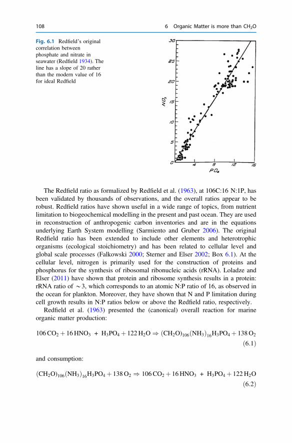
The Redfield ratio as formalized by Redfield et al. (1963), at 106C:16 N:1P, hasbeen validated by thousands of observations, and the overall ratios appear to berobust. Redfield ratios have shown useful in a wide range of topics, from nutrientlimitation to biogeochemical modelling in the present and past ocean. They are usedin reconstruction of anthropogenic carbon inventories and are in the equationsunderlying Earth System modelling (Sarmiento and Gruber 2006). The originalRedfield ratio has been extended to include other elements and heterotrophicorganisms (ecological stoichiometry) and has been related to cellular level andglobal scale processes (Falkowski 2000; Sterner and Elser 2002; Box 6.1). At thecellular level, nitrogen is primarily used for the construction of proteins andphosphorus for the synthesis of ribosomal ribonucleic acids (rRNA). Loladze andElser (2011) have shown that protein and ribosome synthesis results in a protein:rRNA ratio of *3, which corresponds to an atomic N:P ratio of 16, as observed inthe ocean for plankton. Moreover, they have shown that N and P limitation duringcell growth results in N:P ratios below or above the Redfield ratio, respectively.

Redfield et al. (1963) presented the (canonical) overall reaction for marineorganic matter production:

106CO2 þ 16HNO3 + H3PO4 þ 122H2O ) ðCH2O)106ðNH3Þ16H3PO4 þ 138O2

ð6:1Þ

and consumption:

ðCH2O)106ðNH3Þ16H3PO4 þ 138O2 ) 106CO2 þ 16HNO3 + H3PO4 þ 122H2O

ð6:2Þ

Fig. 6.1 Redfield’s originalcorrelation betweenphosphate and nitrate inseawater (Redfield 1934). Theline has a slope of 20 ratherthan the modern value of 16for ideal Redfield

108 6 Organic Matter is more than CH2O

These RKR equations indicate that 138 units of oxygen are required for oxidationof one mole of Redfield organic matter: 106 oxygen molecules to convert CH2O toCO2 and 32 oxygen molecules to convert the NH3 all the way to HNO3. The O2:Ccoefficient for aerobic respiration (including nitrification) is thus 1.3. Primaryproduction based on nitrate (new production) or ammonium (recycled productions)has consequences for the quantity of oxygen released.

The problem with the traditional Redfield ratios as formulated in Eqs. 6.1 and 6.2is that it simplifies marine organic matter into an elementary carbohydrate (CH2O),whereas newly produced marine organic matter is better represented as a mixture ofproteins (*65%), lipids (*19%), and carbohydrates (*16%) and other compounds(pigments and nucleic acids; Hedges et al. 2002; Bianchi and Canuel 2011). Whilesimple carbohydrates are the first molecules formed during carbon fixation, thebiosynthesis of proteins, lipids and polysaccharides results in the loss of hydrogenand oxygen. Hydrogen and oxygen loss results from dehydration, wherein CH2O istransformed into CH2 chains in proteins and lipids. Moreover, there is also hydrogenloss during the transformation of the NH3-group in ideal Redfield organic matter tothe NH-amide group in proteins. Estimates of marine organic matter based onmixing of proteins, lipid, carbohydrates and nucleic acids and using modern ana-lytical tools (Anderson 1995; Hedges et al. 2002), arrive at average compositions ofC106H175O42N16P (Anderson 1995) and C106H177O37N16PS0.4 (Hedges et al. 2002)rather than C106H260O106N16P of the ideal Redfield ratio. This lower oxygen contenthas consequences for the O2:C respiration coefficient. Equation 6.2 can be gener-alized to:

CaHbOvNdPe þ cO2 ) aCO2 þ dHNO3 þ eH3PO4 þ kH2O ð6:3Þ

where c = a + 0.25 b − 0.5v + 1.25d + 1.25 e and k = −0.5d − 1.5 e + 0.5 b.Substitution of these revised marine organic matter compositions in Eq. 6.3 resultsin O2:P ratios of 150 to 154 and an O2:C respiration coefficient (c/a) of*1.43. Thelatter result is consistent with the O2:C ratio of *1.46 obtained from inverseanalysis of water-column nutrient and oxygen changes along isopycnals (Andersonand Sarmiento 1994).

6.2 Non-redfield Organic Matter

The composition of marine particles is rather uniform because phytoplankton andbacteria (and their remains) dominate plankton, and these organisms are primarilymade up of proteins (>50%) supplemented by lipids, carbohydrates, nucleic acidsand pigments. Individual species may deviate from ideal or revised Redfield ratios,but over larger spatial and temporal scales these differences average out. Thecomposition of seagrasses and, in particular, emergent saltmarsh vegetation andmangrove trees deviates from unicellular primary producers: higher C:N and C:Pratios, less proteins and nucleic acids and more structural carbohydrates and lignins.

6.1 Redfield Organic Matter 109

Moreover, there is much more variability in the composition of benthic primaryproducers, particularly in macrophytes. The higher variability is due to tissue dif-ferentiation: compounds involved in photosynthesis and carbon fixation are pri-marily in the leaves and not in the roots. Carbohydrates for storage (e.g. starch) canbe transferred from leaves to rhizomes for long-term storage. These marinemacrophytes re-allocate compounds and essential nutrients over the growing sea-son: e.g. the resorption of nitrogen from senescent leaves and transfer to activegrowing leaves. Structural carbohydrates and lignins are needed for strength to dealwith currents, waves and wind. Lignins are cross-linked phenolic polymers thatoccupy the space between structural carbohydrates, such as cellulose in the cell wallof macrophytes and trees. Polysaccharides are permeable to water, while the morehydrophobic lignins are not. Crosslinking between lignins and celluloses thus notonly strengthens the cell wall but also provides capability to transfer water effi-ciently from roots to the leaves, where evapotranspiration occurs. Thelignin-carbohydrate provided strength and stiffness are needed for saltmarsh plantsand trees to stand and for submerged vegetation to resist currents and waves. Thesepolymers are relatively rich in carbon and poor in nitrogen and phosphorus; this isthe reason why seagrass, salt-marsh plants and in particular mangroves have highC:N and C:P ratios. These polymeric substances are difficult to degrade, with theconsequences that the palatability of seagrasses, marsh vegetation and mangroves isrelatively low (see Fig. 3.10).

6.3 Organic Matter is Food

Organic matter, detritus as well as living biomass, is consumed because it is theprimary source of energy and nutrition for heterotrophic consumers, i.e. it is foodfor animals and a substrate for heterotrophic microbes. Osmotrophic organismseither use dissolved organic matter directly or after extracellular (cell-attached orfree) hydrolysis of polymeric substances into smaller units that can pass the cellmembrane of these microbes. Animals ingest particulate organic matter, part ofwhich is digested, and part is egested. The energy balance for animals is (Welch1968):

I ¼ GþRþE ð6:4Þ

where I is the ingestion of food, G is growth and reproduction of the animal, R isrespiration and E is egestion and excretion (e.g. feces). Food ingested by animals isdigested physically (e.g. chewing, grinding), chemically (by enzymes) and bio-logically (by microbes in the digestion organs) to make it amenable to enter tissues,where it can be used for growth and respiration (energy). This simple equation canbe used to define assimilation (A = G + R), assimilation efficiency (A/I), grossgrowth efficiency (G/I) and net growth efficiency (G/A).


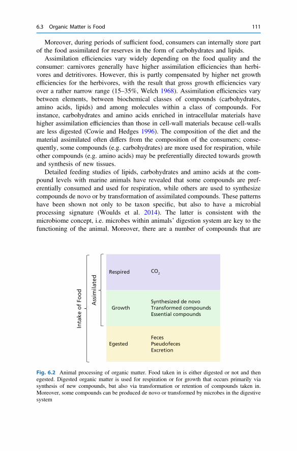
Moreover, during periods of sufficient food, consumers can internally store partof the food assimilated for reserves in the form of carbohydrates and lipids.

Assimilation efficiencies vary widely depending on the food quality and theconsumer: carnivores generally have higher assimilation efficiencies than herbi-vores and detritivores. However, this is partly compensated by higher net growthefficiencies for the herbivores, with the result that gross growth efficiencies varyover a rather narrow range (15–35%, Welch 1968). Assimilation efficiencies varybetween elements, between biochemical classes of compounds (carbohydrates,amino acids, lipids) and among molecules within a class of compounds. Forinstance, carbohydrates and amino acids enriched in intracellular materials havehigher assimilation efficiencies than those in cell-wall materials because cell-wallsare less digested (Cowie and Hedges 1996). The composition of the diet and thematerial assimilated often differs from the composition of the consumers; conse-quently, some compounds (e.g. carbohydrates) are more used for respiration, whileother compounds (e.g. amino acids) may be preferentially directed towards growthand synthesis of new tissues.

Detailed feeding studies of lipids, carbohydrates and amino acids at the com-pound levels with marine animals have revealed that some compounds are pref-erentially consumed and used for respiration, while others are used to synthesizecompounds de novo or by transformation of assimilated compounds. These patternshave been shown not only to be taxon specific, but also to have a microbialprocessing signature (Woulds et al. 2014). The latter is consistent with themicrobiome concept, i.e. microbes within animals’ digestion system are key to thefunctioning of the animal. Moreover, there are a number of compounds that are

Fig. 6.2 Animal processing of organic matter. Food taken in is either digested or not and thenegested. Digested organic matter is used for respiration or for growth that occurs primarily viasynthesis of new compounds, but also via transformation or retention of compounds taken in.Moreover, some compounds can be produced de novo or transformed by microbes in the digestivesystem

6.3 Organic Matter is Food 111

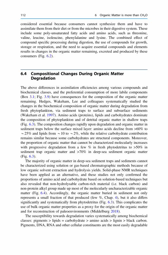
considered essential because consumers cannot synthesize them and have toassimilate them from their diet or from the microbes in their digestive system. Theseinclude some poly-unsaturated fatty acids and amino acids, such as threonine,valine, leucine, isoleucine, phenylalanine and lysine. The combined effect ofcompound specific processing during digestion, the use of compounds for growth,storage or respiration, and the need to acquire essential compounds and elementsresults in changes in the organic matter remaining, excreted and produced by theseconsumers (Fig. 6.2).

6.4 Compositional Changes During Organic MatterDegradation

The above differences in assimilation efficiencies among various compounds andbiochemical classes, and the preferential consumption of more labile components(Box 3.1; Fig. 3.9) have consequences for the composition of the organic matterremaining. Hedges, Wakeham, Lee and colleagues systematically studied thechanges in the biochemical composition of organic matter during degradation fromfresh phytoplankton, via sediment traps to surface and subsurface sediments(Wakeham et al. 1997). Amino acids (proteins), lipids and carbohydrates dominatethe composition of phytoplankton and of detrital organic matter in shallow traps(Fig. 6.3). The composition changes rapidly upon degradation and organic matter insediment traps below the surface mixed layer: amino acids decline from >60% to*25% and lipids from *10 to *2%, while the relative carbohydrate contributionremains similar because some carbohydrates are structural components. Moreover,the proportion of organic matter that cannot be characterized molecularly increaseswith progressive degradation from a few % in fresh phytodetritus to >50% insediment trap organic matter and >70% in deep-sea sediment organic matter(Fig. 6.3).

The majority of organic matter in deep-sea sediment traps and sediments cannotbe characterized using solution or gas-based chromatographic methods because oflow organic solvent extraction and hydrolysis yields. Solid-phase NMR techniqueshave been applied as an alternative, and these studies not only confirmed theproportions of amino acid and carbohydrate based on solution-based techniques butalso revealed that non-hydrolysable carbon-rich material (i.e. black carbon) andnon-protein alkyl group made up most of the molecularly uncharacterizable organicmatter (Fig. 6.4). Accordingly, the organic matter buried in sediment not onlyrepresents a small fraction of that produced (few %, Chap. 4), but it also differssignificantly and systematically from phytodetritus (Fig. 6.3). This complicates theuse of bulk organic matter properties as a proxy for the origin of the organic matterand for reconstruction of paleoenvironments (Middelburg 2018).

The susceptibility towards degradation varies systematically among biochemicalclasses: pigments > lipids = carbohydrate > amino acids > lignin > black carbon.Pigments, DNA, RNA and other cellular constituents are the most easily degradable


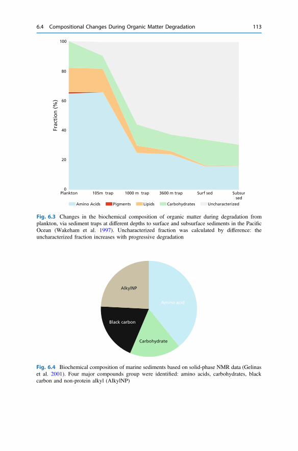
Fig. 6.3 Changes in the biochemical composition of organic matter during degradation fromplankton, via sediment traps at different depths to surface and subsurface sediments in the PacificOcean (Wakeham et al. 1997). Uncharacterized fraction was calculated by difference: theuncharacterized fraction increases with progressive degradation

Fig. 6.4 Biochemical composition of marine sediments based on solid-phase NMR data (Gelinaset al. 2001). Four major compounds group were identified: amino acids, carbohydrates, blackcarbon and non-protein alkyl (AlkylNP)

6.4 Compositional Changes During Organic Matter Degradation 113

compounds, followed by lipids, carbohydrate and amino acids (Fig. 6.3). Whilelignins are degraded in aerobic soils by fungi, these compounds are rather stable inthe marine environments with the consequence that they have high preservationpotential. Besides these differences among biochemical classes, there are also largedifferences among compounds within biochemical classes because of the inherentstructural differences, as well as the macromolecular context. Structural carbohy-drates are more stable than those involved in storage. Amino acids incorporated inlarge proteins are less available for consumers than those dissolved as free aminoacids. Lipid reactivity towards degradation varies widely, as it depends on multiplefactors, including the structure, stereochemistry, head-group, degree of saturation,and ether or ester linkages. While the relative reactivity of various compoundclasses and compounds within a biochemical class is systematic, absolute rates ofdegradation are largely context depending, i.e. identical compounds may have orderof magnitude differences in kinetic parameters depending on the environment.

These systematic changes in organic matter composition due to degradation canbe used to quantify the progress of degradation, or in other words, the degradationhistory. Often used degradation state parameters are intact to total pigment ratios,

05

10152025303540

0

5

10

15

20

25

0

0.5

1

1.5

2

2.5

0

5

10

15

20

25

-2.5 -2 -1.5 -1 -0.5 0 0.5 1 1.5 2 -2.5 -2 -1.5 -1 -0.5 0 0.5 1 1.5 2

Degradation Index Degradation Index

Bal

a+G

aba

(%)

Am

ino

sug

ars

(%)

OC

/SA

mg

C m

-2

Alk

yl C

(%

)

9529

(a) (b)

(d)(c)

Fig. 6.5 Systematic changes in organic matter composition as degradation progresses. Thedegradation index of Dauwe and Middelburg (1998) is based on subtle changes in the amino acidcomposition. Fresh phytoplankton material has positive values, while extensively degradedsedimentary organic matter in deep-sea sediments has values <−1.5. Degradation causes relativeaccumulation of a non-protein amino acids Bala and Gaba and b aminosugars and a decrease inc the organic carbon content per sediment surface area (OC/SA) and d the fraction present asnon-protein alkyl-C. Data are from Dauwe et al. (1999, blue), Gelinas et al. (2001, red) andVandewiele et al. (2009, black)


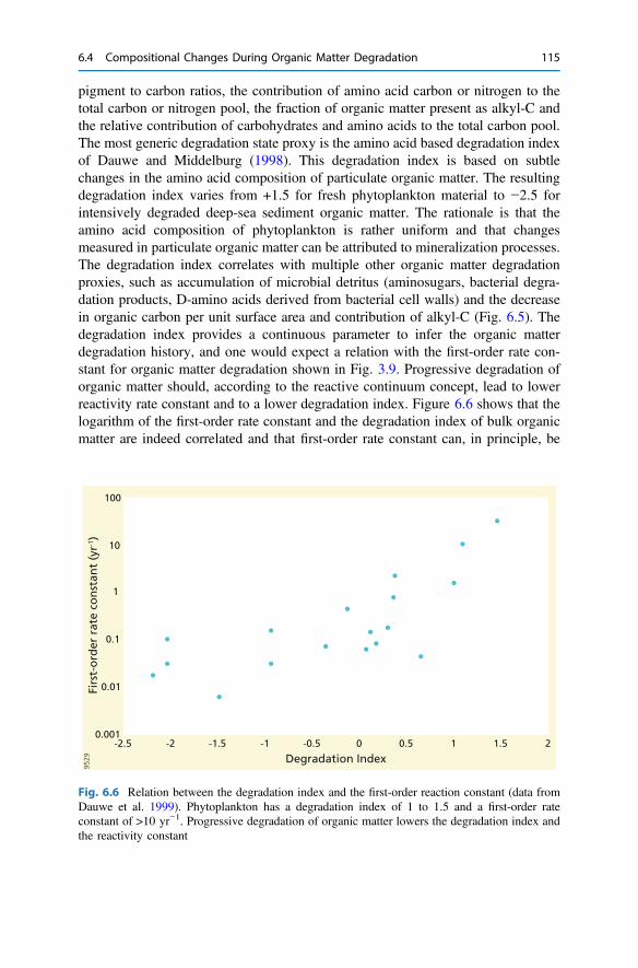
pigment to carbon ratios, the contribution of amino acid carbon or nitrogen to thetotal carbon or nitrogen pool, the fraction of organic matter present as alkyl-C andthe relative contribution of carbohydrates and amino acids to the total carbon pool.The most generic degradation state proxy is the amino acid based degradation indexof Dauwe and Middelburg (1998). This degradation index is based on subtlechanges in the amino acid composition of particulate organic matter. The resultingdegradation index varies from +1.5 for fresh phytoplankton material to −2.5 forintensively degraded deep-sea sediment organic matter. The rationale is that theamino acid composition of phytoplankton is rather uniform and that changesmeasured in particulate organic matter can be attributed to mineralization processes.The degradation index correlates with multiple other organic matter degradationproxies, such as accumulation of microbial detritus (aminosugars, bacterial degra-dation products, D-amino acids derived from bacterial cell walls) and the decreasein organic carbon per unit surface area and contribution of alkyl-C (Fig. 6.5). Thedegradation index provides a continuous parameter to infer the organic matterdegradation history, and one would expect a relation with the first-order rate con-stant for organic matter degradation shown in Fig. 3.9. Progressive degradation oforganic matter should, according to the reactive continuum concept, lead to lowerreactivity rate constant and to a lower degradation index. Figure 6.6 shows that thelogarithm of the first-order rate constant and the degradation index of bulk organicmatter are indeed correlated and that first-order rate constant can, in principle, be

0.001

0.01

0.1

1

10

100

-2.5 -2 -1.5 -1 -0.5 0 0.5 1 1.5 2

Firs

t-o

rder

rat

e co

nst

ant

(yr-1

)

Degradation Index

9529

Fig. 6.6 Relation between the degradation index and the first-order reaction constant (data fromDauwe et al. 1999). Phytoplankton has a degradation index of 1 to 1.5 and a first-order rateconstant of >10 yr−1. Progressive degradation of organic matter lowers the degradation index andthe reactivity constant

6.4 Compositional Changes During Organic Matter Degradation 115

linked to organic matter composition. This does not imply that organic matterchanges are the sole cause, but it does provide avenues to link kinetic biogeo-chemistry and organic geochemistry.

Box 6.1: Ecological stoichiometryThe traditional approach towards food-web and ecosystem functioningfocuses on carbon, i.e. energy, flows and ignores the role of other elementsand the biochemical makeup of organic matter. In other words, the traditionalapproach focuses only on quantity and largely ignores the quality of theorganic matter. This is unfortunate, as all organisms need at least 20 elementsor more and many organisms also have to acquire some essential compoundsfrom the environment or their diet. Ecological stoichiometry explicitly dealswith the flow of nutrients (primarily N, P, but also others) from the envi-ronments via primary producers to herbivores, detritivores and carnivores.

Inspired by the pioneering work of Redfield in the early 20th century,ecologists (Sterner and Elser 2002) have developed the theory of ecologicalstoichiometry in which homeostatis is a central concept. Homeostasis is theproperty of organisms to maintain a constant composition, despite living in avariable environment or feeding on a variable diet (Fig. 6.7). Some organismslack homeostasis, and their cellular nutrient levels reflect that in the envi-ronment (you are what you eat), while strict homeostatic consumers maintaintheir composition. Heterotrophs are, in general, more homeostatic thanautotrophs, but intermediate behavior has been reported. Phytoplankton hasbeen shown to have high flexibility in term nutrients, but suboptimal nutrientcontents come at the expense of performance (e.g. growth rate). Consumersliving on resources that deviate from their tissue composition have multipleways of elemental adjustment: food selection, feeding behavior, regulation ofassimilation and metabolism (e.g. diverting towards respiration or excretion).Most herbivores are richer in N and P than primary producers; this stoi-chiometric mismatch is smaller in aquatic systems than in macrophyte sys-tems in which carbon-rich lignin and structural cellulose are more abundant.Mismatches between the composition of a consumer and its resources hasconsequences for trophic transfer efficiencies and growth rates. The growthrate hypothesis involves a direct link between the growth rate, phosphoruscontent and ribosomes: i.e. high P content imply high RNA and thus highpotential for growth. Ecological stoichiometry links the elements via com-pounds to the functioning of organisms and organism-scale processes to theglobal biogeochemical cycles.


References

Anderson LA (1995) On the hydrogen and oxygen content of marine phytoplankton. Deep Sea ResPart I 42:1675–1680

Anderson LA, Sarmiento JL (1994) Redfield ratios of remineralization determined by nutrient dataanalysis. Glob Biogeochem Cycles 8:65–80

Bianchi TS, Canuel EA (2011) Chemical biomarkers in aquatic ecosystems. Princeton UniversityPress

Cowie GL, Hedges JI (1996) Digestion and alteration of the biochemical constituents of a diatom(Thalassiosira weissflogii) ingested by an herbivorous zooplankton (Calanus pacificus).Limnol Oceanogr 41:581–594

Dauwe B, Middelburg JJ (1998) Amino acids and hexosamines as indicators of organic matterdegradation state in North Sea sediments. Limnol Oceanogr 43:782–798

Dauwe B, Middelburg JJ, Herman PMJ, Heip CHR (1999) Linking diagenetic alteration of aminoacids and bulk organic matter reactivity. Limnol Oceanogr 44:1809–1814

Falkowski PG (2000) Rationalizing elemental ratios in unicellular algae. J Phycol 36:3–6Gelinas Y, Baldock JA, Hedges JI (2001) Carbon composition of immature organic matter from

marine sediments: effect of oxygen exposure on oil generation potential. Science 294:145–148Hedges JI, Baldock JA, Gélinas Y, Lee C, Peterson ML, Wakeham SG (2002) The biochemical

and elemental compositions of marine plankton: a NMR perspective. Mar Chem 78:47–63Loladze I, Elser JJ (2011) The origins of the Redfield nitrogen-to-phosphorus ratio are in a

homoeostatic protein-to-rRNA ratio. Ecol Lett 14:244–250Middelburg JJ (2018) Reviews and syntheses: to the bottom of carbon processing at the seafloor.

Biogeosciences 5:413–427

9529 Resource ratio

Co

nsu

mer

rat

io

Homeostasis

Homeostasis

No homeostasis

You are what y

ou eat

Fig. 6.7 Generalised stoichiometric pattern relating consumer (N:P, C:N, etc.) ratio to resourceratios. Organisms lacking homeostasis reflect the ratio of their resource (dashed 1:1 line), whilestrictly homeostatic organisms maintain their composition irrespective of the environment or theirdiet (horizontal line)

References 117

Redfield AC (1934) On the proportions of derivatives in sea water and their relation to thecomposition of plankton. James Johnson memorial volume. University of Liverpool,Liverpool, UK, pp 176–192

Redfield AC (1958) The biological control of chemical factors in the environment. Am Sci46:205–221

Redfield AC, Ketchum BH, Richards FA (1963) The influence of organisms on the composition ofseawater. In: Hill MN (ed) The sea. Interscience, pp 26–77

Sarmiento J, Gruber N (2006) Ocean biogeochemical dynamics. Princeton University Press,pp 526

Sterner RW, Elser JJ (2002) Ecological stoichiometry: the biology of elements from molecules tothe biosphere. Princeton University Press

Vandewiele S, Cowie G, Soetaert K, Middelburg JJ (2009) Amino acid biogeochemistry andorganic matter degradation state accross the Pakistan margin oxygen minimum zone. Deep SeaRes II 56:376–392

Wakeham SG, Lee C, Hedges JI, Hernes PJ, Peterson ML (1997) Molecular indicators ofdiagenetic status in marine organic matter. Geochim Cosmochim Acta 61:5363–5369

Welch HE (1968) Relationships between assimilation efficiencies and growth efficiencies foraquatic consumers. Ecology 49:755–759

Woulds C, Middelburg JJ, Cowie GL (2014) Alteration of organic matter during infaunalpolychaete gut passage and links to sediment organic geochemistry. Part II: fatty acids andaldoses. Geochimica Cosmochimica Acta 136:38–59





Documents

Jack J. Middelburg Marine Carbon Biogeochemistry A Primer ... · roots can be traced back to early scientists documenting how living organisms transformed chemical substances, such