[J. Res. Natl. Inst. Stand. Technol. Mathematics and ... · be considered to be the results of property measure-ments, though of a logical system rather than a physical one. ... Twelve

Volume 106, Number 1, January–February 2001Journal of Research of the National Institute of Standards and Technology

[J. Res. Natl. Inst. Stand. Technol. 106, 293–313 (2001)]

Mathematics and Measurement

Volume 106 Number 1 January–February 2001

Ronald F. Boisvert, Michael J.Donahue, Daniel W. Lozier,Robert McMichael, and Bert W.Rust

National Institute of Standards andTechnology,Gaithersburg, MD 20899-0001

[email protected]@[email protected]@[email protected]

In this paper we describe the role thatmathematics plays in measurement sci-ence at NIST. We first survey the historybehind NIST’s current work in this area,starting with the NBS Math Tables projectof the 1930s. We then provide examplesof more recent efforts in the application ofmathematics to measurement science, in-cluding the solution of ill-posed inverseproblems, characterization of the accu-racy of software for micromagnetic model-ing, and in the development and dissemi-nation of mathematical reference data.Finally, we comment on emerging issues

in measurement science to which mathe-maticians will devote their energies incoming years.

Key words: deconvolution; digital li-braries; history of NBS; linear algebra;mathematical reference data; mathemati-cal software; micromagnetic modeling;parameter estimation; software testing;scientific computing.

Available online: http://www.nist.gov/jres

1. Introduction

Mathematics plays an important role in the science ofmetrology. Mathematical models are needed to under-stand how to design effective measurement systems, andto analyze the results they produce. Mathematical tech-niques are used to develop and analyze idealized modelsof physical phenomena to be measured, and mathemati-cal algorithms are necessary to produce practical solu-tions on modern computing devices. Finally, mathemat-ical and statistical techniques are needed to transformthe resulting data into useful information.

Applied mathematics has played a visible role atNBS/NIST since the Math Tables project in the 1930s,and formal mathematical and statistical organizationshave been part of NBS/NIST since the establishment ofthe National Applied Mathematics Laboratory in 1947.Among these organizations was the NBS Institute forNumerical Analysis (1947-54), which has been credited

as the birthplace of modern numerical analysis. TheNIST Mathematical and Computational Sciences Divi-sion (MCSD) is the modern successor to these NBS/NIST organizations.

In this paper we indicate some of the important con-tributions of mathematics to NBS/NIST measurementprograms during the past 60 years. We then provideexamples of more recent efforts in the application ofmathematics to measurement science. This includeswork in the the solution of ill-posed inverse problems,characterization of the accuracy of software for micro-magnetic modeling, and in the development and dissem-ination of mathematical reference data. Finally, we com-ment on emerging issues in measurement science towhich mathematicians will devote their energies incoming years.

293


2. History

2.1 Early Developments

Mathematical research at NBS began in the late1930s when NBS Director Dr. Lyman J. Briggs con-ceived a project for the computation of tables of mathe-matical functions of importance in applications. Theresulting Mathematical Tables Project was located inNew York and administered by the Works Projects Ad-ministration. The project, under the direction of ArnoldN. Lowan, employed mathematicians and a large num-ber of additional staff to carry out the necessary compu-tations by hand. From 1938 to 1946, 37 volumes of theNBS Math Tables Series were issued, containing tablesof trigonometric functions, the exponential function,natural logarithms, probability functions, and relatedinterpolation formulae [23].

Such tabulated values of mathematical functions canbe considered to be the results of property measure-ments, though of a logical system rather than a physicalone. Thus, the Bureau’s first foray into mathematicalresearch was intimately involved with measurement.

The contributions of applied mathematics to the wareffort in the 1940s fueled a widespread recognition ofthe importance of mathematical research to the attain-ment of national goals. In 1946, the Chief of NavalResearch suggested that NBS consider the establishmentof a national laboratory for applied mathematics. NBSDirector Dr. Edward U. Condon was enthusiastic aboutthe idea, and the National Applied Mathematics Labora-tory (NAML) was established at NBS the following yearwith John H. Curtiss as its director. The program for theNAML was to have two main components: numericalanalysis and statistical analysis [10]. The NAML hadfour main operating branches, the Institute for Numeri-cal Analysis (INA), the Computation Laboratory, theMachine Development Laboratory, and the StatisticalEngineering Laboratory. The first of these was housedat the University of California Los Angeles, while theremaining were located at NBS in Washington. Thesewere the organizational beginnings of today’s Informa-tion Technology Laboratory at NIST, which continues towork in applied mathematics, statistics, and high perfor-mance scientific computation, among other areas.

The original prospectus for the NAML proposed thatit serve as a computation center for the Federal govern-ment. Computing equipment for large-scale computa-tions were not readily available in the late 1940s, ofcourse. NAML was the first organization in the world tobuild and put into service a successful large scale, elec-tronic, fully automatic stored-program digital comput-ing system [10]. This system, the Standards Eastern Au-tomatic Computer (SEAC), designed and built in

collaboration with the NBS Electronics Division, wasput into continuous operation in May 1950. Its originalconfiguration included a 512-word mercury delay linememory and teletype input-output. Despite its stagger-ing 12 000 diodes and 1000 vacuum tubes, the SEACoperated reliably 77 % of the time during its first threeyears of operation. A machine of somewhat differentdesign, the Standards Western Automatic Digital Com-puter (SWAC), was built at the INA in Los Angeles.These unique computational facilities allowed mathe-maticians from NBS and other institutions to performcalculations that spurred the development of modernnumerical analysis. The name NAML was dropped in1954 in favor of “Applied Mathematics Division.”

2.2 Institute for Numerical Analysis

Approximately three-fourth’s of the output of NAMLduring its first 5 years was in numerical analysis. Re-search in this area was emphasized due to the surgingneed for appropriate mathematical methods for use inexploiting the nation’s emerging digital computing ca-pability. Dr. Mina Rees, Director of the MathematicalSciences Section of the Office of Naval Research, whichprovided more than 80 % of the funding for the NAML,is credited with this vision. The center of this activitywithin NAML was the INA, an organization that, in avery real sense, pioneered modern numerical analysis.

The list of INA Directors and permanent staff duringits period of operation (1947-54) reads like a Who’sWho of modern numerical analysis, including FormanS. Acton, George E. Forsythe, Magnus R. Hestenes,Fritz John, Cornelius Lanczos, Derrick H. Lehmer, J.Barkeley Rosser, Charles B. Tompkins, and Wolfgang R.Wasow. These were augmented by many visiting facultyappointments, junior researchers, and graduate fellows.

Among INA’s areas of emphasis were:

• Solution of linear systems of equations• Linear programming• Computation of eigenvalues of matrices• Finite difference methods for partial differential equa-

tions• Monte Carlo methods• Numerical solution of ordinary differential equations• Numerical methods for conformal mapping• Asymptotic expansions• Interpolation and quadrature

The story of the development of Krylov subspacemethods for the solution of systems of linear algebraicequations illustrates the far-reaching impact of theINA’s technical program. The conjugate gradient al-gorithm is the earliest example of this class of methods.

294


It is a method of iterative type which does not requireexplicit storage or manipulation of a matrix (only theability to apply the underlying operator to any givenvector). As such, it is ideal for the solution of very largeand sparse systems. For symmetric (or Hermitian) posi-tive definite systems it has the property that it convergesin finite time (after n iterations for a system of order n );nevertheless, because of its iterative nature it can oftenbe stopped earlier, providing acceptable results at mod-erate cost.

The first complete description of the conjugate gradi-ent method appeared in a paper published in the NBSJournal of Research by Magnus R. Hestenes and EduardStiefel [19]. Hestenes was a member of the NBS INA,and Stiefel a visiting researcher from the Eidgenossis-chen Technischen Hochschule (ETH) in Zurich. Theirpaper remains the classic reference on this method.Other INA staff, such as Cornelius Lanczos and MarvinStein, also made fundamental early contributions to thedevelopment of the method.

While there was much early interest in the algorithm,it went into eclipse in the 1960s as naive implementa-tions failed on the increasingly larger problems whichwere being posed. Interest in the conjugate gradientmethod surged again in the 1970s when researchersdiscovered new variants and successful techniques forpreconditioning the problem (i.e., premultiplication by acarefully chosen easily invertible matrix) to reduce thenumber of iterations. Today, these methods are the stan-dard techniques employed for the solution of large linearsystems. Citation searches for the term conjugate gradi-ent turn up more than one million articles in which theterm is used during the last 25 years. Krylov subspacemethods were identified as one of the top ten algorithmsof the century by Computing in Science and Engineer-ing 1 [13] in January 2000. An account of the history ofthe conjugate gradient method can be found in Ref. [18].

NBS was required to give up the administration of theINA in June 1954, a result of new Department of De-fense rules which torpedoed funding arrangements withthe Office of Naval Research. This was one of the unfor-tunate events in the wake of the AD-X2 battery additivecontroversy in which NBS found itself embroiled from1948 to 1953. The INA was transferred to UCLA, butby this time most INA members had taken positions inindustry and in universities. More information about theINA can be found in the accounts of Todd and Hestenes[20, 34].

1 A publication of the IEEE Computer Society and the AmericanInstitute of Physics.

2.3 Handbook of Mathematical Functions

With the establishment of the NAML in 1947 theMath Tables Project was transferred to the NBS Compu-tation Laboratory. Subsequent tabulations were issued inthe newly established NBS Applied Mathematics Series(AMS) of monographs, whose earliest issue providedtables of Bessel functions [2].

In 1956 NBS embarked on another ambitious pro-gram which was a natural outgrowth of its work onmathematical tables. Led by Dr. Milton Abramowitz,who was then Chief of the Computation Laboratory, theproject would develop a compendium of formulas,graphs, and tables which would provide practitionerswith the most important facts needed to use the growingcollection of important mathematical functions in appli-cations. Among these are the Bessel functions, hyperge-ometric functions, elliptic integrals, probability distri-butions, and orthogonal polynomials.

With substantial funding from the National ScienceFoundation, many well-known experts in the field wereenlisted as authors and editorial advisors to compile thetechnical material. By the summer of 1958, substantialwork had been completed on the project. Twelve chap-ters had been written, and the remaining ones were wellunderway. The project experienced a shocking setbackone weekend in July 1958 when Abramowitz suffered afatal heart attack. Irene Stegun, the Assistant Chief ofthe Computation Laboratory, took over management ofthe project. The exacting work of assembling the manychapters, checking tables and formulas, and preparingmaterial for printing took much longer than anticipated.Nevertheless, the 1046-page Handbook of MathematicalFunctions, with Formulas, Graphs, and MathematicalTables was finally issued as AMS Number 55 in June1964 [1].

The public reaction to the publication of the Hand-book was overwhelmingly positive. In a preface to theninth printing in November 1970, NBS Director LewisBranscomb wrote

The enthusiastic reception accorded the“Handbook of Mathematical Functions” is littleshort of unprecedented in the long history of math-ematical tables that began when John Napier pub-lished his tables of logarithms in 1614.

The Handbook has had enormous impact on scienceand engineering. The most widely distributed NBS/NIST technical publication of all time, the governmentedition has never gone out of print (more than 145 000have been sold), and it has been continuously availableas a Dover reprint since 1965. The Handbook’s citationrecord is also remarkable. More than 23 000 citations

295


have been logged by Science Citation Index (SCI) since1973. Remarkably, the number of citations to the Hand-book continues to grow, not only in absolute numbers,but also as a fraction of the total number of citationsmade in the sciences and engineering. During the mid1990s, for example, about once every 1.5 hours of eachworking day some author, somewhere, made sufficientuse of the Handbook to list it as a reference.

2.4 Mathematical Analysis

A number of difficult mathematical problemsemerged in the course of developing the Handbookwhich engaged researchers in the Applied MathematicsDivision for a number of years after its publication. Twoof these are especially noteworthy, the first having to dowith stability of computations and the second with pre-cision.

Mathematical functions often satisfy recurrence rela-tions (difference equations) that can be exploited incomputations. If used improperly, however, recurrencerelations can lead to ruinous errors. This phenomenon,known as instability, has tripped up many a computationthat appeared superficially to be straightforward. Theerrors are the result of subtle interactions in the set of allpossible solutions of the difference equation. Frank W. J.Olver, who wrote the Handbook’s chapter on Besselfunctions of integer order, studied this problem exten-sively. In a paper published in 1967 [28], Olver providedthe first (and only) stable algorithm for computing alltypes of solutions of a difference equation with threedifferent kinds of behavior: strongly growing, stronglydecaying, and showing moderate growth or decay. Thiswork is reflected today in the existence of robust soft-ware for higher mathematical functions.

Another important problem in mathematical compu-tation is the catastrophic loss of significance caused bythe fixed length requirement for numbers stored in com-puter memory. Morris Newman, who co-authored theHandbook’s chapter on combinatorial analysis, soughtto remedy this situation. He proposed storing numbersin a computer as integers and performing operations onthem exactly. This contrasts with the standard approachin which rounding errors accumulate with each arith-metic operation. Newman’s approach had its roots inclassical number theory: First perform the computationsmodulo a selected set of small prime numbers, wherethe number of primes required is determined by theproblem. These computations furnish a number of localsolutions, done using computer numbers represented inthe normal way. At the end, only one multilength com-putation is required to construct the global solution (theexact answer) by means of the Chinese Remainder The-orem. This technique was first described in a paper by

Newman in 1967 [26]; it was employed with great suc-cess in computing and checking the tables in Chap. 24of the Handbook. Today, this technique remains a stan-dard method by which exact computations are per-formed.

In the 1960s NBS mathematicians also made pioneer-ing efforts in the development and analysis of graph-the-oretic algorithms for the solution of combinatorial opti-mization problems. Jack Edmonds did ground-breakingwork in the analysis of algorithms and computationalcomplexity, focusing on the establishment of measuresof performance which distinguished practical al-gorithms from impractical ones [15]. This work pro-vided a solid foundation for algorithms which have be-come the mainstay of operations research. In recognitionof this work, Edmonds received the 1985 John VonNeumann prize from the Institute for Operations Re-search and the Management Sciences (INFORMS).

2.5 Scientific Computing

As computing systems became more powerful, NBSscientists were increasingly drawn to the use of compu-tational methods in their work. Results of experimentalmeasurements needed to be analyzed, of course, butmore and more scientists were using mathematical mod-els to help guide the measurement process itself. Mod-els could be developed to simulate experimental systemsin order to determine how best to make the measure-ments or how to correct for known systematic errors.Finally, mathematical models could be used to under-stand physical systems that were extremely difficult tomeasure. Increasingly, NBS mathematicians were beingconsulted to help develop such models and to aid indevising computational methods of solving them.

While the NBS Applied Mathematics Division hadalways engaged in collaborative work with NBS scien-tists, during the 1970s through the 1990s this becamethe central theme of its work (and that of its successororganizations, the Center for Applied Mathematics, andthen the Computing and Applied Mathematics Labora-tory). Examples of such long-term collaborations in-clude the study of combustion, smoke and gas flowduring fires [4], the modeling of semiconductor devices[5], and the modeling of alloy solidification processes[9].

In the 1980s the newly formed NBS Scientific Com-puting Division began the development of a repositoryof mathematical software tools to aid NBS scientists inthe development and the solution of models. Amongthese were the NIST Core Mathematics Library (CM-LIB) and the joint DOE/NIST Common Math Library(SLATEC) [8]. The growing collection of such tools wasindexed in the Guide to Available Mathematical Soft-

296


ware (GAMS) [6], which continues to provide the com-putational science community with information on, andaccess to, a wide variety of tools, now via a convenientWeb interface (http://gams.nist.gov/).

2.6 Current Mathematical Research

Today the NIST Mathematical and ComputationalSciences Division (MCSD) is focused on (1) assuringthat the best mathematical methods are applied in solv-ing technical problems of the NIST Laboratories, and(2) targeted efforts to improve the environment for com-putational science within the broader research commu-nity. The Division provides expertise in a wide variety ofareas, such as nonlinear dynamics, stochastic methods,optimization, partial differential equations (PDE), com-putational geometry, inverse problems, linear algebra,and numerical analysis. This is applied in collaborativeresearch projects performed in conjunction with otherNIST Laboratories. Substantial modeling efforts are un-derway in the analysis of the properties of materials, incomputational electromagnetics, and in the modeling ofhigh-speed machine tools, for example. Modeling ef-forts are supported by work in the development of math-ematical algorithms and software in areas such as adap-tive solution of PDEs, special functions, Monte Carlomethods, deconvolution, and numerical linear algebra.

In response to needs of the wider community, MCSDhas developed a number of Web-based information ser-vices, such as the Guide to Available Mathematical Soft-ware, the Matrix Market (see Sec. 4.1), the Java Numer-ics site, and the Digital Library of MathematicalFunctions (see Sec. 5). In addition, staff members areinvolved in standardization efforts for fundamental lin-ear algebra software and for numerical computing inJava.

Current work of the Division is described in its Webpages at http://math.nist.gov/. The following sectionsprovide further details of several of these projects whichhave particular relevance to the measurement sciences.

3. Mathematics of Physical Metrology

In physical metrology it is often necessary to fit amathematical model to experimental results in order torecover the quantities being measured. In some cases thedesired variables can be measured more or less directly,but the measuring instruments distort the measuredfunction so much that mathematical modeling is re-quired to recover it. In other cases the desired quantitiescannot be measured directly and must be inferred byfitting a model to the measurements of variables dynam-ically related to the ones of interest.

3.1 Deconvolution

An example of measurements of the first type wasbrought to Bert Rust’s attention by Jeremiah Lowney[24] of the NIST Semiconductor Electronics Division.The measurements were linear scans by a scanning elec-tron microscope (SEM) across a semiconductor chip onwhich a circuit had been etched. The goal was to mea-sure the location of features on the chip with uncertaintylevels of 10 nanometers (nm) or smaller. The measure-ments are modeled by a system of linear, first kindintegral equations,

y0(xi ) = �xi+4�

xi�4�

K (� � xi )yt(� )d� + �i ,

(1)i = 1, 2, ..., 301,

where the variables x and � are both distances (in nm)along the scan, yt(� ) is the desired “true” signal strengthat distance � , and the values y0(xi ) are observed signalstrengths on a mesh x1, x2, ..., x301, with a mesh-width�x = xi+1 � xi = 2 nm. These measured values fail togive a faithful discrete representation of the unknownfunction yt(� ) because they are smoothed by the mea-surement process and because of the additive randommeasurement errors �i . The incident scanning beam isnot infinitely sharp. The beam intensity is thought tohave a Gaussian profile

K (� � xi ) =1

�2��exp��

12� 2 (� � xi )2�, (2)

with a “beam diameter” d = 2.56� = 37.5 nm. The ob-served signal is thus the sum of a convolution of the truesignal yt(� ) with this Gaussian function and the randommeasuring errors.

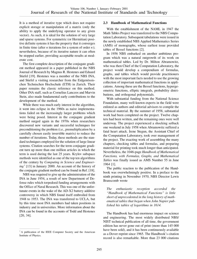
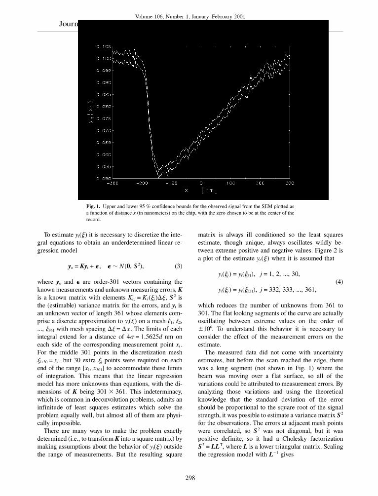
The measurements for a scan across a sharp step-likeedge are shown in Fig. 1. At the left of the plot, theelectron beam is incident on (and perpendicular to) apresumably flat surface. The electrons penetrate thesemiconductor and excite a roughly spherical distribu-tion of secondary emissions. Most of these secondaryelectrons are reabsorbed by the material but a signifi-cant fraction escape into the vacuum chamber above.These escaped electrons are collected by an electrode togenerate the current that gives the measured signal. Asthe primary beam crosses the edge, more and more ofthe emitted electrons come from the lower surface, andmany of these are reabsorbed by the wall. Thus there isa sharp drop in the signal. Even when the incident beamhas moved well clear of the wall, its “shadow” persistsfor a large distance, causing a slow recovery of thesignal to its original level.

297


Fig. 1. Upper and lower 95 % confidence bounds for the observed signal from the SEM plotted asa function of distance x (in nanometers) on the chip, with the zero chosen to be at the center of therecord.

To estimate yt(� ) it is necessary to discretize the inte-gral equations to obtain an underdetermined linear re-gression model

yo = Kyt + � , � � N (0, S 2), (3)

where yo and � are order-301 vectors containing theknown measurements and unknown measuring errors, Kis a known matrix with elements Ki,j = Ki (�j )�� , S 2 isthe (estimable) variance matrix for the errors, and yt isan unknown vector of length 361 whose elements com-prise a discrete approximation to yt(� ) on a mesh �1, �2,..., �361 with mesh spacing �� = �x . The limits of eachintegral extend for a distance of 4� = 1.5625d nm oneach side of the corresponding measurement point xi .For the middle 301 points in the discretization mesh�i+30 = xi , but 30 extra �j points were required on eachend of the range [x1, x301] to accommodate these limitsof integration. This means that the linear regressionmodel has more unknowns than equations, with the di-mensions of K being 301 � 361. This indeterminacy,which is common in deconvolution problems, admits aninfinitude of least squares estimates which solve theproblem equally well, but almost all of them are physi-cally impossible.

There are many ways to make the problem exactlydetermined (i.e., to transform K into a square matrix) bymaking assumptions about the behavior of yt(� ) outsidethe range of measurements. But the resulting square

matrix is always ill conditioned so the least squaresestimate, though unique, always oscillates wildly be-tween extreme positive and negative values. Figure 2 isa plot of the estimate ye(� ) when it is assumed that

yt(�j ) = yt(�31), j = 1, 2, ..., 30,(4)

yt(�j ) = yt(�331), j = 332, 333, ..., 361,

which reduces the number of unknowns from 361 to301. The flat looking segments of the curve are actuallyoscillating between extreme values on the order of�106. To understand this behavior it is necessary toconsider the effect of the measurement errors on theestimate.

The measured data did not come with uncertaintyestimates, but before the scan reached the edge, therewas a long segment (not shown in Fig. 1) where thebeam was moving over a flat surface, so all of thevariations could be attributed to measurement errors. Byanalyzing those variations and using the theoreticalknowledge that the standard deviation of the errorshould be proportional to the square root of the signalstrength, it was possible to estimate a variance matrix S 2

for the observations. The errors at adjacent mesh pointswere correlated, so S 2 was not diagonal, but it waspositive definite, so it had a Cholesky factorizationS 2 = LLT, where L is a lower triangular matrix. Scalingthe regression model with L�1 gives

298


Fig. 2. Linear least squares estimate of yt, assuming fixed constant extensions outside the range ofmeasurements, plotted as a function of distance � (in nanometers) from the center of the record.

L�1yo = L�1Kyt + L�1� ,(5)

L�1� � N (0, I301),

where I301 is the order-301 identity matrix. The fact thatthe random errors in this rescaled model are indepen-dently distributed with the standard normal distributionsimplifies the analysis of the effects of those errors onthe estimated solution.

Let ye be an estimate for yt and

r = L�1(yo � Kye) (6)

be the corresponding residual vector. Comparing thisexpression with Eq. (5) suggests that ye is acceptableonly if r is a plausible sample from the (L�1� )-distribu-tion. This means that the elements of r should be dis-tributed N (0,1), and the sum of squared residuals rTrshould lie in some interval [301 � �602,301 + �602], with | |< 2. This last condition followsfrom the fact that

�301

i=1

(L�1� )2i = �TS�2� � 2(301). (7)

hence

�{�TS�2�} = 301, Var {�TS�2�} = 2 � 301. (8)

When the assumptions of Eq. (4) are imposed on thescaled model of Eq. (5), L�1K becomes a 301 � 301

matrix, so, in theory, the unique least squares estimatesatisfies L�1yo = L�1Kye exactly. Because of roundingerrors, calculations on a real computer did not give anexact 0 residual vector, so the calculated sum of squaredresiduals was 8.20 � 10�4 which is neglible when com-pared to the expected value 301. This means that almostall of the variance in the measured record is explainedby the model. A significant part of that variance is dueto measurement errors, so the least squares estimate hascaptured variance that properly belongs in the residuals.This misplaced variance is amplified by the ill-condi-tioning to produce the wild oscillations in Fig. 2.

One approach to resolving the indeterminacy in Eq.(5) and stabilizing the estimated solution is to imposephysically motivated a priori constraints in order to re-duce the size of the set of feasible solutions. For manymeasurement problems, nonnegativity is an appropriateand often powerful constraint, especially when comput-ing confidence intervals for the estimate. Consider thecase of computing upper and lower confidence boundsfor each of the 361 elements of the estimated solution.Let the chosen confidence level be 100� % (with0 < � < 1), and define

�L�1(yo � Ky )�2 = (yo � Ky )T S�2(yo � Ky ). (9)

The problem then is, for j = 1, 2, ..., 361, to compute

y loj = min �eT

j y � �L�1(y0 � Ky )�2 = 2�, (10)y�0

299


y upj = max �eT

j y � �L�1(y0 � Ky )�2 = 2�, (11)y�0

where ej is the unit vector whose j th element is one, and 2 is a statistical parameter which must be chosen toguarantee that

Pr{y loj � eT

j yt � y upj } � � . (12)

In 1972, Rust and Burrus [32] conjectured, and in 1994Rust and O’Leary [33] proved that valid 100� % confi-dence intervals are obtained if

2 = �min + 2, (13)

where

�min = min ��L�1(yo � Ky )�2�, (14)y�0

and is the � -percentile for the N (0,1) distribution.The calculation of each of the bounds in Eqs. (10) and

(11) is a separate quadratic programming problem. In1972, Rust and Burrus [32] gave heuristic arguments toshow that each pair y lo

j and y upj were the two roots of the

piecewise quadratic equation

�j (� ) = min ��L�1(yo � Ky )�2 �eTj y = ��. (15)

y�0

In 1986 O’Leary and Rust [27] gave a formal proof ofthis fact and presented an efficient algorithm calledBRAKET-LS for calculating those roots. It has beensuccessfully used for radiation spectrum unfolding byusers both at NIST [14] and other laboratories [16].

An inspection of Fig. 1 reveals that, for the presentproblem, the constraints yj � 0.045 are even more ap-propriate than nonnegativity. These constraints can bereduced to nonnegativity by a simple transformation ofvariables, but unfortunately, as indicated by Fig. 3, theydo not constrain the solution set enough to overcome theindeterminacy. The vertical axis has been truncated inorder to exhibit the behavior of the estimate in the inter-val �300 � � � 300. The maximum ye(� ) would haveto be increased to the value 70.0 to accommodate theoff-scale excursions on both ends of the plot.

Fortunately, there are more powerful constaintswhich are appropriate for this problem and which can bereduced to nonnegativity by a transformation of vari-ables. For a simple edge, the signal should be monoton-ically non-increasing before it “bottoms out” andmonotonically non-decreasing during the recovery. It iseasy to design a matrix T so that the linear transforma-tion yt = Tz converts the constraints z � 0 into the de-sired monotonicity constraints on the elements of yt.One can then use BRAKET-LS on the transformedproblem with unknown solution z . Figure 4 gives theupper and lower two standard deviation bounds obtainedwhen the turning point is chosen to be �109 = �144 nm.The bounds explode at each end of the record, but within

Fig. 3. Constrained linear least squares estimate, with constraints yj � 0.045, j = 1, 2, ..., 361,plotted as a function of distance � (in nanometers) from the center of the record.

300


the interval of measurement [�300, +300] nm, the con-fidence intervals are comparable in size to those for themeasured signal (cf. Fig. 1). The most difficult part ofdesigning the matrix T is determining the point wherethe non-increasing constraint should be changed to anon-decreasing one. If a gap is left between the twosegments, the uncertainties explode in that gap, but the

bounds in the two segments are not very sensitive to thesmall variations in the turning point, so good results canbe obtained by trial and error.

The quality of the confidence intervals in Fig. 4 is agood recommendation for the corresponding estimatewhich is plotted in Fig. 5. The estimate is plotted as asolid curve and the measured data as a dashed curve.

Fig. 4. Monotonicity constrained, one-at-a-time, 95 % confidence interval bounds for the truesignal plotted as a function of the distance � (in nanometers) from the center of the record.

Fig. 5. Monotonicity constrained estimate (solid curve) and observed signal (dashed curve) plottedas functions of distance (in nanometers) from the center of the record.

301


The edge definition for the estimate is much sharperthan that for the data. The sharp drop begins at�92 = �178 nm and reaches the minimum level at�94 = �174 nm. The drop is almost, but not exactly,linear. The single intermediate point at �93 = �176 nmfalls slightly to the left of the straight line connecting thetwo extreme points. The uncertainties indicated in Fig.4 are not sufficiently small to permit the conclusion thatthe variation in the interval �178 � � � �174 repre-sents a real departure from a vertical drop rather than anuncertainty in the location of that drop. In the lattercase, the results indicate that the best estimate for thatlocation is (176 � 2) nm, and in either case the originalgoal of measuring the location of the drop to an accu-racy of 10 nm or smaller has been attained.

A surprise in the estimate in Fig. 5 was the staircaseform of the recovery segment. This is unlikely to be theresult of an inappropriate assumption of monotonicity.Had the monotonicity assumptions not been correct, thelikely result would have been null sets for the feasibleregions in the constrained estimation problems of Eqs.(10) and (11). The bounds in Fig. 4, which were calcu-lated independently from the estimate, also display ahint of this staircase effect. One should not dismiss theidea that the steps indicate a real layering of the materialin the etched chip. Studies with scanning tunneling mi-croscopes [17, 21] of etched surfaces on silicon haverevealed terraces with width distributions very similar tothe distribution of widths of the steps in the figure. Butmore work should be done before drawing any conclu-sions about the cause of these steps because the interpre-tation of SEM scans is not simple or easy.

3.2 Parameter Estimation

Another important mathematical modeling problemin physical metrology is fitting a system of ordinarydifferential equations (ODEs) to a set of observed timeseries data which are corrupted by measurement errors.The desired quantities, which are unknown parametersin the ODEs, cannot be measured directly. Their valuesmust be inferred from the fit to the measurements ofdynamically related variables.

An example of a problem like this was brought to BertRust by Robert W. Ashton of the NIST BiotechnologyDivision. The problem arose in connection with a studyof the ability of anhydrothrombin (AT), a derivative ofthe enzyme thrombin (T), to compete with thrombin forthe binding of a potent thrombin inhibitor hirudin (H).The chemical equations for the reactions are

(AT)+

�2

T + H →← (TH)�1

�4 ↓ ↑ �3

(ATH)

where (TH) is the thrombin-hirudin complex, (ATH) isthe anhydrothrombin-hirudin complex, and �1, �2, �3,and �4 are the rates of the indicated reactions.

Two experiments were performed. In the firstthrombin and hirudin were allowed to react, forming the(TH) complex, until equilibrium was established, andthen, at time t = 0, an aliquot of anhydrothrombin wasadded. Then, over the next 33 hours, aliquots were re-moved at eight unequally spaced times and assayed forthrombin activity. This experiment was repeated threetimes, so the final data consisted of an average value andan estimate of its uncertainty at each of the eight timepoints. These data are are plotted on the upper curve inFig. 6 with the concentrations of thrombin in units ofpercent activity.

In the second experiment, anhydrothrombin andhirudin were allowed to come to equilibrium with the(ATH) complex, and at time t = 0 an aliquot of thrombinwas added. Then again, thrombin assays were taken ateight unequally spaced times. This experiment was alsorepeated three times to get averages and uncertainties.These data are plotted on the lower curve in Fig. 6. Notethat the thrombin concentrations in the two experimentsconverge to the same equilibrium value.

The mathematical problem is to estimate �1, �2, �3,and �4 from the 16 measured thrombin concentrations.It can be shown that

�4 = ��2�3

�1, (16)

where � = 0.4312, so the ODEs describing the kineticsof the reactions can be written

dTdt

= �1(TH) � �2(T)(H),

d(AT)dt

= �3(ATH) � ��2�3

�1(AT)(H),

dHdt

= �1(TH) + �3(ATH)

(17)

��2(T)(H) � ��2�3

�1(AT)(H),

d(TH)dt

= �2(T)(H) � �1(TH),

d(ATH)dt

= ��2�3

�1(AT)(H) � �3(ATH).

302


Fig. 6. Simultaneous fits to the two thrombin concentration time series.

Ashton and his colleagues [35] had already found anapproximate solution to this problem using two pertur-bation expansions, but they wanted an independent con-firmation of their result.

Equations (17) are nonlinear ODEs which do not havea closed form solution. To estimate the vector � = (�1,�2, �3)T it is necessary to combine a numerical ODEintegrator with a nonlinear fitting program to minimizethe sum of squared residuals

� (� ) = �2

k=1�8

i=1

[T ck,i (� ) � T o

k,i ]2, (18)

where k is the experiment number, i is the index ofmeasurement times, the T o

k,i are the measured values, andthe T c

k,i (� ) are the corresponding predicted values ob-tained by numerically integrating the ODEs.

The nonlinear fitting program begins with initial esti-mates � (0) and iterates to a local minimum of Eq. (18).On each iteration it must integrate the system [Eq. (17)]with the current values of � . It also requires the partial

derivatives��1

,��2

, and��3

in order to compute the

step for the next iteration. To obtain these, it must alsointegrate the system of 15 variational equations ob-tained by taking partial derivatives of each of the ODEsin Eq. (17) with respect to �1, �2, and �3.

Fortunately the initial values for the solutions to theODEs in Eq. (17) were known exactly. For many prob-lems of this type, the initial values are either unknownor are measured values, subject to the same kind of

measurement errors as the other measured points. Insuch cases, it is necessary to treat them as unknownparameters to be determined by the fit. The fitting prob-lem is then much more difficult. Even for relativelysimple problems like the present one, the response func-tion [Eq. (18)] has many local minima corresponding tovalues of � which do not give good fits to the data. It isabsolutely necessary to pick starting estimates � (0) closeenough to the correct local minimum to give a good fit.The difficulty of finding such values increases veryrapidly as the number of unknown parameters increases.

The estimates obtained by simultaneously fitting thedata from the two experiments were

�1 = (1.62 � .23) � 10�5 s�1,

�2 = (6.0 � 1.6) � 107 s�1,

�3 = (3.01 � .31) � 10�5 s�1.

The corresponding solutions to the ODEs are plotted assmooth curves in Fig. 6. The fits accounted for 99.4 %of the combined total variance in the two measuredrecords. These results agree quite well with those ob-tained by Ashton and his colleagues, so the goal of theexercise was attained. But it should be noted that thelower curve does not fit its data as well as the uppercurve, and that there is no guarantee that there is notanother local minimum of Eq. (18) which would giveeven better fits.

303


4. Testing and Evaluation of Software

The need for measurement as an aid to understandingis not unique to physical systems. As software systemsincrease in complexity, many of their properties havebecome difficult to know a priori. Thus, experimentaltechniques for evaluating performance characteristics ofsoftware, such as speed and accuracy, have come intowidespread use. We will describe several recent projectswhich are providing tools for the measurement of prop-erties of mathematical algorithms and software.

A frequently applied method for the testing of numer-ical software is to exercise it on a battery of representa-tive problems. Often such problems are generated ran-domly, insuring that a large number of test cases can beapplied. Unfortunately, this is rarely sufficient for seri-ous numerical software testing. Errors or numerical dif-ficulties typically occur for highly structured problemsor for those near to the boundaries of applicability of theunderlying algorithm. These parts of the domain arerarely sampled in random problem generation, andhence testing must also be done on problem sets thatillustrate particular behaviors. These are often quite dif-ficult to produce, and, thus, researchers often exchangesample problem sets. Such data sets serve a variety ofadditional purposes:

1. Defining the state-of-the-art.2. Characterizing industrial-grade applications.3. Catalyzing research by posing challenges.4. Providing a baseline of performance for software

developers.5. Providing data for users who want to gain confidence

in software.

Unfortunately, these collections are often lost when theunderlying technology is picked up by the commercialsector, leaving software developers and users without animportant tool to use in judging the capability of theirproducts. In this section we will describe recent work inthe NIST Mathematical and Computational SciencesDivision to address such needs in core linear algebrasoftware and in micromagnetic modeling software.

4.1 The Matrix Market

The decomposition, solution and eigenanalysis of sys-tems of linear equations are fundamental problems inscientific computation for which new algorithms andsoftware packages are continually being developed. Thestudy of measures of inherent difficulty for the solutionof such problems, so-called condition numbers , occu-pied mathematicians at the NBS INA in the 1950s [10].Today, linear systems of equations that are represented

by sparse matrices remain of paramount importance. Asparse matrix is a matrix in which most elements arezero. Figure 7 is a sparsity plot for such a matrix; thedots show where nonzeros are located. Problems of thistype arise in modeling based on partial differentialequations, such as in fluid flow and structural analysis.The behavior of algorithms and software for such prob-lems is highly dependent on the sparsity structure andthe numerical properties derived from the underlyingproblem. As a result, in order to make reliable, repro-ducible and quantitative assessments of the value of newalgorithmic developments it is useful to have a commoncollection of representative problems through whichmethods can be compared. Researchers in this area haveexchanged problem sets of this type informally for sometime. One of the difficulties with such collections is thattheir size and diversity makes them unwieldy to manageand use effectively. As a result, such collections have notbeen used as much as they should, and matrices usefulfor testing are not easy to find.

Developments in network communications in-frastructure, such as the World Wide Web, have providednew possibilities for improving access to and usabilityof test corpora of this type. The NIST Matrix Market issuch a Web-based repository of matrices for use in thecomparative analysis of algorithms and software for nu-merical linear algebra. More than 500 matrices of sizeup to 90 449 � 90 449 from a wide variety of applica-tions are made available in the Matrix Market. Matricesare gathered together into sets. Matrices in a set arerelated by application area or contributed from a singlesource. Sets are grouped further into collections, such asthe well-known Harwell-Boeing collection. Individualmatrices may be stored explicitly as dense or sparsematrices, or may be available implicitly via a code thatgenerates them. Matrix generators are either run atNIST remotely via Web-based form, or run locally as aJava applet in a Web browser. In other cases, Fortrancode may be downloaded for inclusion in a local testingapplication. Available matrices are of a wide variety oftypes, e.g., real, complex, symmetric, nonsymmetric,Hermitian. Some are only representations of nonzeropatterns. Others include supplementary data such asright-hand sides, solution vectors, or initial vectors foriterative solvers. We store matrices and associated mate-rial one-per-file, in both the Harwell-Boeing format, aswell as in a new Matrix Market format. Software forreading and writing such matrices in Fortran, C, andMatlab2 are provided.

2 Certain commercial equipment, instruments, or materials are identi-fied in this paper to foster understanding. Such identification does notimply recommendation or endorsement by the National Institute ofStandards and Technology, nor does it imply that the materials orequipment identified are necessarily the best available for the purpose.

304


Fig. 7. Structure plot of a sparse matrix. Dark spots indicate the position of nonzero matrixelements.

For each matrix we provide a summary Web pageoutlining the properties of the matrix and displaying agraphical representation of its properties. Graphics in-clude sparsity plots such as shown above, and three-di-mensional representations in Virtual Reality ModelingLanguage (VRML) format which can be manipulatedgraphically in a Web browser. Spectral portraits, whichillustrate the sensitivity of matrix eigenvalues, are alsoavailable in many cases. Similarly, we have developed aWeb page for each set that gives its background (e.g.,source and application area), references, and a thumb-nail sketch of each matrix’s nonzero pattern. We main-tain a separate database that contains all of the informa-tion on these pages in a highly structured form. Thisallows us to manipulate the data in various ways; forexample, all of the Web pages for matrices and sets areautomatically generated from this database. The data-base also supports both structured and free-text re-trieval. The Matrix Market search tool, for example,allows users to locate matrices with particular specialproperties, e.g., all real symmetric positive definite ma-trices with more than 10 000 rows and less than 0.1 %density.

The Matrix Market has supported linear algebra re-searchers and software developers since 1997. About

500 matrices are downloaded from the site each month.Further details can be found in Ref. [7] or at the Web sitehttp://math.nist.gov/MatrixMarket/.

4.2 Micromagnetic Modeling

The purpose of micromagnetic calculations is to com-pute the behavior of the magnetization in a magneticmaterial in response to a sequence of applied magneticfields. This kind of modeling is important for the designof magnetic devices such as magnetic recording headsand media, and for the microstructural design of mag-netic materials. If micromagnetic calculations are tosubstitute for physical experiments, the software em-ployed must first be validated. Careful comparison toexperimental results is one way to do this. Such a projectis quite ambitious, requiring (1) valid solutions for themodel equations, (2) good values of materials parame-ters, and (3) careful experimental design and assessmentof experimental errors.

The work we have done is focused solely on the firstof these issues. The mathematical model for micromag-netism is derived from the atomic scale physics of elec-tron spin and orbital interactions, and is thought to bevalid over length scales large enough that the magnetiza-

305


tion can be approximated by a continuous field of three-dimensional vectors of constant magnitude. This micro-magnetic model consists of a set of nonlinear partialdifferential equations often referred to as Brown’s equa-tions .

Taking the model as a given, we set out to test theoutput of various computational methods. We have donethis through development of standard problems to besolved by the micromagnetics community as a whole,and by developing a public micromagnetic code that canserve as a reference and testbed for computational tech-niques.

Testing the validity of computed results really tests anumber of separate but related things:

• the validity of algorithms,• correct implementation of algorithms (bug free code),

and• valid use of the algorithms.

These three items require a skilled mathematician, askilled programmer, and a skilled operator familiar withthe limitations of the algorithms. Sometimes, but notalways, one person is responsible for all three of theseskills.

Our experience with standard problems and referencecode has been a consequence of our formation and facil-itation of the Micromagnetic Modeling Activity Group( MAG), which was created to work on standard prob-lems in micromagnetics and on publicly available micro-magnetic code.

Our contact with the community of researchers in thefield of magnetism, and in micromagnetics in particular,has been mainly through the use of “piggy-back” work-shops held as evening sessions at major internationalmagnetism conferences. We began by convening a steer-ing committee of representatives from industry,academia and government labs to plan our first work-shop. Following this meeting the importance of thesteering committee has diminished, and we have beenformulating plans based mostly on feedback, often byquick show-of-hands opinion polls at the workshops.

4.2.1 Standard Problems

It is important to achieve a balance in problem defini-tion between over-specification of the problem and lackof focus. In the extreme limit of over-specification, allaspects of solving the problem are determined, and par-ticipants have no freedom to select differing solutionmethods. Effectively, all participants are forced to runthe same program, and comparisons of the contributedsolutions can reveal only potential compiler or CPUerrors. On the other extreme, characterized by lack of

focus, participants solve significantly different prob-lems, and again nothing is learned about the validity ofthe solutions.

Because we want to test solution methods, in ourstandard problems we have specified the material ge-ometry, material parameters and applied field direc-tions. All other parameters, including the discretizationscheme, discretization size, dynamic behavior and thespecific applied field values are left open.

For problems where the results are to be published inarchival journals, we try to keep the scope of the prob-lem small so that the standard problem results can be asmall part of a larger paper containing variations on theproblem. Otherwise, we felt that reviewers and editorsmight fail to see the value of results that had beenpreviously calculated.

Our first standard problem was proposed, specified,and posted before anyone had attempted to solve it. Theproblem was conceptually simple, and the parameterscorresponded to the parameters of working devices. Inretrospect, the first standard problem was poorly se-lected because it proved to be too computationally de-manding for participants to compute a valid solution.

Learning from this mistake, we made the second stan-dard problem specification scalable by selection of aparameter value. For small parameter values, the prob-lem was less computationally demanding than for largeparameter values. We expected solutions which closelyagree for small parameter values and that diverged as theparameter value increases.

The most important consideration in collecting solu-tions to a standard problem is that the demands on par-ticipants time must be kept to a minimum. We have usedtwo methods of collecting solutions. With our first stan-dard problem, we recognized that initial results weredisagreeing rather severely. Recognizing that such re-sults could prove embarrassing to individuals, or even tocorporations, the results were posted in anonymousfashion on a collection of web pages, so results could becompared without learning the source of any particularsolution. Even under the protection of anonymity, lobby-ing was often required to obtain solutions.

Following our experience with the first standard prob-lem and having proposed two different, simpler standardproblems, we switched to publication of standard prob-lem results in regular archival journals. Workshop at-tendees felt that this would allow researchers to getcredit for their work through normal channels. In addi-tion to publication, we requested data from those pub-lishing papers on the standard problems to post on the MAG web page where results could be comparedside-by-side.

306


4.2.2 Reference Software

The public code project complements the standardproblem suite by providing freely available softwarewith source code that can be used to provide expandeddetail on solutions to the standard problems, and providereference results to other problems. It runs on a widerange of machines, and presents a graphical user inter-face that allows it to be used by the non-specialist. Inparticular, it is a useful aid to understanding experimen-tal results.

In developing reference micromagnetic software wehad several goals in mind. The code needed to be pow-erful and flexible enough for in-house research, and toprovide sample results for the standard problems. On theother hand, an issued raised in the first MAG meetingwas the importance of having a code available that ex-perimentalists could use to help interpret their results,without a major investment of time to learn to use thecode. We also wanted a modular code that could be usedas a development platform for new researchers in thefield of micromagnetics.

To provide portability and an easy to use graphicalinterface, we decided to write the user interface code inthe Tcl/Tk scripting language, while the core of themicromagnetic solver would be written in C++ for mod-ularity and extensibility. To make the code widely avail-

able, we created a web site where regular alpha and betareleases of both full source code and executables wouldbe placed.

4.2.3 Results

The activities of MAG, including complete standardproblem specifications and results are documented athttp://www.ctcms.nist.gov/~rdm/mumag.html. Thepublic reference code is available for download at http://math.nist.gov/oommf/.

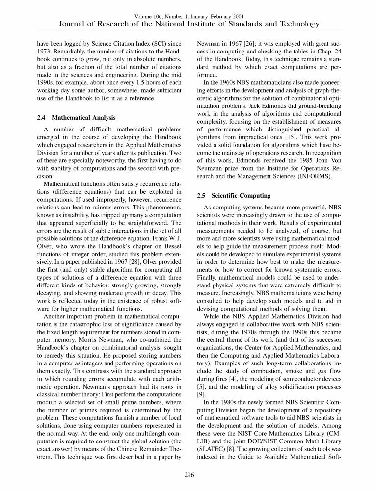
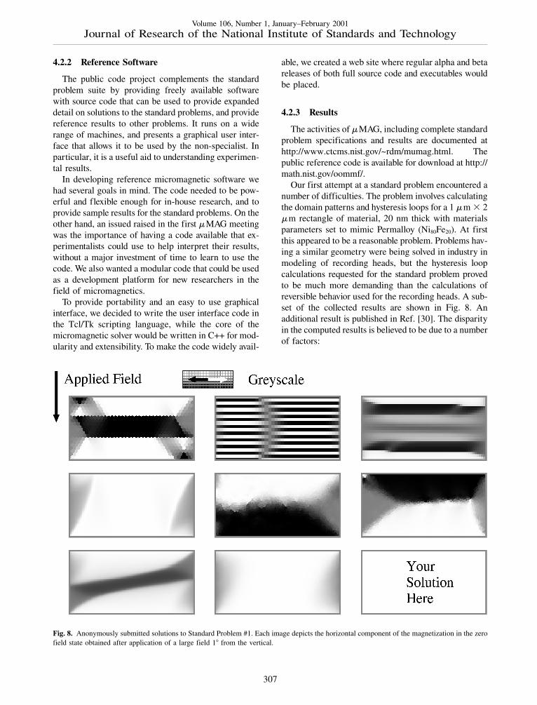
Our first attempt at a standard problem encountered anumber of difficulties. The problem involves calculatingthe domain patterns and hysteresis loops for a 1 m � 2 m rectangle of material, 20 nm thick with materialsparameters set to mimic Permalloy (Ni80Fe20). At firstthis appeared to be a reasonable problem. Problems hav-ing a similar geometry were being solved in industry inmodeling of recording heads, but the hysteresis loopcalculations requested for the standard problem provedto be much more demanding than the calculations ofreversible behavior used for the recording heads. A sub-set of the collected results are shown in Fig. 8. Anadditional result is published in Ref. [30]. The disparityin the computed results is believed to be due to a numberof factors:

Fig. 8. Anonymously submitted solutions to Standard Problem #1. Each image depicts the horizontal component of the magnetization in the zerofield state obtained after application of a large field 1� from the vertical.

307


• Proximity of specified field values to critical values.The maximum field requested was very close to thefield required for complete saturation, and applyingthe field 1 � off axis was insufficient to break thesymmetry of the problem

• Large problem dimensions relative to intrinsic lengthscales. The exchange length for Permalloy is approxi-mately 5 nm. The number of computational grid cellsrequired to discretize down to this length scale wasprohibitive.

Standard Problem #2 is a bar of magnetic material,with aspect ratios 5:1:0.1. The material is specified bymagnetization Ms and exchange stiffness parameter A .The intrinsic length scale, the exchange length, is givenby � = �2A / 0M 2

s . Magnetocrystalline anisotropy isset to zero. All length scales can be expressed in unit of� and all fields can be expressed in units of Ms. With theapplied field oriented in the [1,1,1] direction relative tothe principle axes of the bar, the problem is to calculatethe remnant magnetization and coercivity of the bar asa function of the bar width. The problem is expected tobecome progressively more challenging as the bar di-mensions are increased relative to � . Results have beenpublished in the open literature [3, 12, 22, 25] includingan analytical solution for the limit of small dimensions[12]. A representative plot is shown in Fig. 9.

Standard Problem #3, like problem #2, involves anobject with variable dimensions, but is more suitable fora 3D code. The object is a cube with magnetization, Ms,exchange stiffness parameter, A , and magnetocrystallineanisotropy constant Ku = 0.1 � 1

2 0M 2s , with the easy

direction parallel to a principle axis of the cube. Thereis no applied field. For very small cubes, the minimumenergy state is expected to be nearly uniform magnetiza-tion, and for a large cube the minimum energy state isexpected to involve a number of domains. The problemis to find the cube edge length, L , such that the nearlyuniform “flower” state has the same energy as a “vortexstate” (Fig. 10). Solutions for this problem agree well,ranging from L = 8.469� to L = 8.52� , with one paperpublished in the open literature [29] and the others de-scribed on the web site listed above.

The problem specification assumes that the “flower”and “vortex” states are the two lowest energy states forthe cube. However, in one of the submitted solutions, theexistence of another “twisted flower” state is describedthat has the lowest energy near L = 8.5.

Standard Problem #4 is a “proposed” problem, cur-rently posted for comments from the community. It isprimarily intended as a test for dynamic micromagneticcalculations. The material is a 500 nm � 125 nmrectangle of material, 3 nm thick, with parameters de-signed to mimic Permalloy. The dynamics of the magne-tization have been specified as the Landau-Lifshitz-Gilbert equation.

Fig. 9. Coercive field as a function of the bar width for Standard Problem #2. The labels refer to theauthors of Refs. [3, 12, 22, 25].

308


Fig. 10. Schematic drawings of the expected “flower” and “vortex”magnetization states for Standard Problem #3.

Starting with magnetization in a specified zero-field“s-state,” fields are applied instantaneously to reversethe magnetization, and the evolution of the magnetiza-tion is traced as the magnetization comes to equilibriumin its new state. Calculations for two switching fields arespecified, applied 170 � and 190 � from the long axis ofthe rectangle of material. Because the s-state is asym-metric, for one of these fields the magnetization willreverse by rotating in the same direction throughout thesample. The computation is expected to be more diffi-cult for the other applied field, since preliminary com-putations have shown that the magnetization initiallyrotates in different directions in different parts of thesample, creating vortices and domain walls that aremore difficult to resolve.

4.2.4 Outcomes

We have developed several standard problems inmicromagnetics, and have enlisted the help of the micro-magnetics community in generating results to thesestandard problems. As our experience has increased, wehave become better at proposing tractable, well-definedproblems. As a result, we have been able to shift fromcollecting anonymous solutions to the problems, wherethe identity of the solution author is protected, to solu-tions that are subject to peer review and published in thenormal way. This transition is important since it allowsthe problem solvers to get credit and financial supportfor their work through normal channels. The standardproblems are now in a state where they can be used ina limited way for their intended purpose, to detect errorsin micromagnetic computer software.

The first public release of the reference micromag-netic software occurred in January 1998. The softwarewas developed by Michael Donahue and Donald Porter,with some early contributions by Robert McMichael.We have released upgrades on a regular basis since thattime. The documentation, which is included with eachrelease and is available on the web site in online form,

has been published as a NIST report [11]. The softwareruns on a wide variety of Unix and Windows computers,and has contributed to at least 10 papers in refereedjournals. We have also used the reference code toprovide solutions to the standard problems. This is espe-cially useful as interested parties can determine addi-tional details about the solutions not included in thereports by downloading the software and replicating theresults. This is also a good practice exercise for learningto use the code.

Results from the standard problems also feed backand influence the public code. For example, the firstthree submitted solutions to Standard Problem #2 wereStreibl, McMichael, and Diaz (refer to Fig. 9). We ex-pected the solutions to agree for small values of d /lex,and although close, there appeared to be a systematicdisagreement between the Streibl results and the othertwo. We examined our results (McMichael) moreclosely, and determined that there was a bias in thecalculation of the demagnetization field near the edgesof the bar [12]. We implemented an improved demagne-tization module, and submitted new results (Donahue)that agree closely with the Streibl results, and the ana-lytic result in the small particle limit.

5. Digital Library of MathematicalFunctions

In Sec. 2.3 we described the development of the NBSHandbook of Mathematical Functions . The functionswhose properties were laid out in this reference workcontinue to play a critical role in applied mathematicalmodeling. As a result, practitioners still need ready ac-cess to a reliable source of information about mathemat-ical functions, which accounts for the Handbook’s con-tinued popularity. Nevertheless, it is now out-of-date inmany respects. Since its publication, numerous ad-vances in related fields of mathematics have been made:

• New functions have entered the realm of practicalimportance, e.g., q-series.

• New fields of application have emerged, e.g., in non-linear dynamics.

• Analytical developments have occurred, e.g., inasymptotics.

• New properties, e.g., integral representations and ad-dition formulas, have been discovered.

• Numerical developments, e.g., interval analysis andPade approximations, have occurred.

• Computer algebra and symbolic processing havecome into wide use.

• An enormous increase in computing power has madeobsolete standard numerical processes of the 1950s,

309


such as table-making and interpolation, while increas-ing the value of others.

• Comprehensive software packages have been con-structed for working and computing with functions.

At the same time, dissemination of information isbeing revolutionized by the rapid development of theInternet and World Wide Web. A modern successor tothe Handbook should provide new capabilities unavail-able in print media, such as:

• Generic representation of mathematical entities suchas formulas, graphs, tables and diagrams.

• Advanced search, with the ability to locate formulasbased on mathematical subexpressions.

• Downloading of mathematical entities into documentprocessors.

• Importing of formulas directly into symbolic comput-ing systems.

• Continuous updating to incorporate corrections, addi-tions and extensions.

• Maintenance of communication channels betweenusers and developers, with a public record of usage.

• Support for external application modules to providetutorials, application notes or research monographs infields that use mathematical functions.

• Recommendations of algorithms and software forcomputing functions, with links to sources.

• Generation of numerical tables and graphs for user-specified ranges of input.

NIST has begun the process of completely rewritingthe Handbook for presentation as an on-line resourcewith many of these features. The result will be the NISTDigital Library of Mathematical Functions (DLMF).The project entails (a) gathering all pertinent mathemat-ical information, (b) constructing a state-of-the-art ref-erence database with all necessary tools for long-termmaintenance, (c) presenting validated reference infor-mation on the Web, and (d) developing application mod-ules in quantum mechanics, electromagnetism, and anadaptive learning system for mathematical functions.

The DLMF project is being managed by four princi-pal editors at NIST: Daniel Lozier, Frank Olver, CharlesClark, and Ronald Boisvert. They are assisted by a panelof 10 associate editors representing expertise in specialfunctions, numerical analysis, combinatorics, computeralgebra, physics, chemistry, and statistics. The DLMFwill have 38 chapters:

1. Mathematical and Physical Constants2. Algebraic and Analytical Methods3. Asymptotic Approximations4. Numerical Methods

5. Computer Algebra6. Elementary Functions7. Gamma Function8. Exponential Integral, Logarithmic Integral, Sine

and Cosine Integrals9. Error Functions, Dawson’s Integral, Fresnel Inte-

grals10. Incomplete Gamma Functions and Generalized Ex-

ponential Integral11. Airy and Related Functions12. Bessel Functions13. Struve Functions and Anger-Weber Functions14. Confluent Hypergeometric Functions15. Coulomb Wave Functions16. Parabolic Cylinder Functions17. Legendre Functions and Spherical Harmonics18. Hypergeometric Functions19. Generalized Hypergeometric Functions and Meijer

G-Function20. q-Hypergeometric Functions21. Classical Orthogonal Polynomials22. Other Orthogonal Polynomials23. Elliptic Integrals24. Theta Functions25. Jacobian Elliptic Functions26. Weierstrass Elliptic and Modular Functions27. Bernoulli and Euler Numbers and Polynomials28. Zeta and Related Functions29. Combinatorial Analysis30. Functions of Number Theory31. Statistical Methods and Distributions32. Mathieu Functions and Hill’s Equation33. Lame Functions; Spheroidal Wave Functions34. Heun Functions35. Painleve Transcendents36. Integrals with Coalescing Saddles37. Wavelets38. 3j, 6j, 9j Symbols

The second through fifth chapters will provide back-ground material in mathematical and numerical analy-sis. The remaining chapters deal with individual func-tions or classes of functions. An emphasis will be placedon a concise presentation of the mathematical propertiesof the functions, including formulas, visualizations,methods of computation, and representative applica-tions. Pointers to state-of-the-art software for computingthe functions will also be supplied. Detailed tables offunction values, which occupied more than half of theoriginal Handbook, will not be included The last sixchapters contain material on functions which were notrepresented in the original Handbook, and all the chap-ters are enlarged. Tables aside, the DLMF will containtwice the material found in the original Handbook.

310


The technical material is being developed by some 50external participants. Of these, authors under contract toNIST will complete a survey of the literature as the basisfor their chapters. After chapters are approved by theEditorial Board they will be carefully checked by inde-pendent external validators, also under contract to NIST.

The DLMF will be made available in a highly interac-tive Web site maintained by NIST (see Fig. 11). Eachlabeled item (e.g., section, formula, table) will havemetadata associated with it, both to aid in searching, andto provide readers with further information such as linksto original references and generalizations. Interactivetools for visually exploring functions will be supplied asJava applets or as VRML worlds. Providing certifiedtables of function values on demand for each of thefunctions in the DLMF is beyond the scope of the cur-rent project. However, this is recognized as a need, andit will be demonstrated for several of the functions in theDLMF.

A prototype of the Digital Library can be inspected athttp://dlmf.nist.gov/. Completion of the system is ex-pected in 2002.

6. Future Trends in Mathematics at NIST

The widespread availability of substantial computa-tional power will increase the demand for mathematicaland computational modeling. As more and more peopleattempt to exploit such methodology, there will begreater need for specialized, but flexible, computationalproblem-solving environments for science and engineer-ing applications [31]. These will be built from mathe-matical components which must have a higher degree ofreliability than those in common use today. Mathemati-cal research will be needed in the development of fast,reliable, adaptive and self-validating algorithms for awide variety of problems. As the development of math-ematical software components moves from the researchcommunity to the commercial sector there will also bea critical need for techniques and tools to assess theaccuracy and reliability of mathematical systems andcomponents. NIST is a natural home for the develop-ment of measurement technology in this area.

Increased computational modeling capabilities willhave an even greater impact on future NIST measure-

Fig. 11. Windows illustrating the capabilities of the Digital Library of Mathematical Functions.

311


ment programs. As higher fidelity models are proposedand efficient solution techniques developed, there comesthe real possibility of replacing many physical measure-ments by virtual measurements performed on mathe-matical models. Before this can occur, however, sub-stantial efforts must be made to more carefullycharacterize models and sources of error so that theprecision and accuracy of virtual measurements can bequantitatively assessed in the same way as physical mea-surements. Of course, such technology would not makeexperiment-based metrology obsolete. Instead, experi-mental measurements would be targeted to the calibra-tion and validation of mathematical models.

Acknowledgments

This article surveys many projects underway withinthe NIST Information Technology Laboratory. Its au-thors represent only a portion of those with significantinvolvement in these projects. The following is a listingof the contributors to the projects described. MatrixMarket: Ronald Boisvert, Roldan Pozo, Karin Reming-ton, Robert Lipman, Bruce Miller. Digital Library ofMathematical Functions : Daniel Lozier, Frank Olver,Charles Clark, Ronald Boisvert, Bruce Miller, BonitaSaunders, Qiming Wang, Marjorie McClain, Joyce Con-lon, Bruce Fabijonas. Micromagnetic Modeling:Michael Donahue, Jason Eicke, Donald Porter, RobertMcMichael. In this paper, Sec. 3 was written by BertRust, and section Sec. 4.2 was written by Michael Don-ahue and Robert McMichael.

7. References

[1] Milton Abramowitz and Irene E. Stegun, eds., Handbook ofMathematical Functions, with Formulas, Graphs, and Mathe-matical Tables, National Bureau of Standards Applied Mathe-matics Series, Vol. 55, U.S. Government Printing Office, Wash-ington, D.C. (1964).

[2] Tables of Bessel Functions Y0 (x ), Y1 (x ), K0 (x ), K1 (x ),0 � x � 1, National Bureau of Standards Applied MathematicsSeries, Vol. 1, U.S. Government Printing Office (1948).

[3] T. Schrefl B. Streibl and J. Fidler, Dynamic FE simulation of MAG standard problem No. 2, J. Appl. Phys. 85, 5819–5821(1999).

[4] Howard R. Baum, O. A. Ezekoye, Kevin B. McGrattan, andRonald G. Rehm, Mathematical-modeling and computer-simu-lation of fire phenomena, Theo. Comp. Fluid Dyn. 6, (2–3),125–139 (1994).

[5] James L. Blue and Charles L. Wilson, Two-dimensional analy-sis of semiconductor-devices using general-purpose interactivePDE software, IEEE Trans. Electron Devices 30 (9), 1056—1070 (1983).

[6] Ronald F. Boisvert, Sally E. Howe, and David K. Kahaner,GAMS—a framework for the management of scientific soft-ware, ACM Trans. Math. Software 11, 313–355 (1985).

[7] Ronald F. Boisvert, Roldan Pozo, Karin Remington, Richard F.Barrett, and Jack J. Dongarra, Matrix Market: a web resource fortest matrix collections, in Quality of Numerical Software, As-sessment and Enhancement, Ronald F. Boisvert, ed., Chapman& Hall, London (1997) pp. 125–137.

[8] Bill L. Buzbee, The SLATEC common mathematical library, inSources and Development of Mathematical Software, Wayne R.Cowell, ed., Prentice-Hall, Englewodd Cliffs, NJ (1984) pp.302–318.

[9] Sam R. Coriell, Geoffrey B. McFadden, and Robert F. Sekerka,Cellular growth during directional solidification, Annu. Rev.Mater. Sci. 15, 119–145 (1985).

[10] John H. Curtiss, The National Applied Mathematics Laborato-ries of the National Bureau of Standards: A progress reportcovering its first five years of existance, Ann. Hist. Comput. 11(2), 69–98 (1989).

[11] M. J. Donahue and D. G. Porter, OOMMF User’s Guide, Ver-sion 1.0, NISTIR 6376, National Institute of Standards andTechnology, Gaithersburg, MD, September 1999.

[12] M. J. Donahue, D. G. Porter, R. D. McMichael, and J. Eicke,Behavior of MAG standard problem No. 2 in the small particlelimit, J. Appl. Phys. 87, 5520–5522 (2000).

[13] Jack Dongarra and Francis Sullivan, Guest editors’ introduction:the top ten algorithms, Comput. Sci. Eng. 2 (1), 22–23 (2000).

[14] K. C. Duvall, S. M. Seltzer, C. G. Soares, and B. W. Rust,Dosimetry of a nearly monoenergetic 6 to 7 MeV photon sourceby NaI(Tl) scintillation spectrometry, Nucl. Instrum. MethodsPhys. Res. Sec. A 272, 866–870 (1988).

[15] Jack Edmonds, Paths, trees, and flowers, Canad. J. Math. 17,449–467 (1965).

[16] Bruce A. Faddegon, Len Van der Zwan, D. W. O. Rogers, andC. K. Ross, Precision response estimation, energy calibration,and unfolding of spectra measured with a large NaI detector,Nucl. Instrum. Methods Phys. Res. Sec. A 301, 138–149 (1991).

[17] Jaroslav Flidr, Yi-Chiau Huang, Theresa A. Newton, andMelissa A. Hines, The formation of etch hillocks during step-flow etching of Si(111), Chem. Phys. Lett. 302, 85–90 (1999).

[18] Gene H. Golub and Dianne P. O’Leary, Some history of theconjugate gradient and Lanczos algorithms, SIAM Rev. 31, 50–102 (1989).

[19] Magnus R. Hestenes and Eduard Stiefel, Methods of conjugategradients for solving linear systems, J. Res. Natl. Bur. Stand.(U.S.) 49, 409–436 (1952).

[20] Magnus R. Hestenes and John Todd, NBS-INA—the Institutefor Numerical Analysis—UCLA 1947–1954, NIST SpecialPublication 730, National Institute of Standards and Technol-ogy, U.S. Government Printing Office, Washington, D.C.(1991).

[21] Yi-Chiau Huang, Jaroslav Flidr, Theresa A. Newton, andMelissa A. Hines, Effects of dynamic step-step repulsion andautocatalysis on the morphology of etched Si(111) surfaces,Phys. Rev. Lett. 80 (20), 4462–4465 (1998).

[22] L. Lopez-Diaz, O. Alejos, L. Torres, and J. I. Iniguez, Solutionsto micromagnetic standard problem No. 2 using square grids, J.Appl. Phys. 85, 5813–5815 (1999).

[23] Arnold N. Lowan, The Computation Laboratory of the NationalBureau of Standards, Scripta Math. 15, 33–63 (1949).

[24] Jeremiah R. Lowney, Applications of Monte Carlo simulationsto critical dimension metrology in a SEM, Scanning Microsc.10, 667–678 (1997).

[25] R. D. McMichael, M. J. Donahue, D. G. Porter, and Jason Eicke,Comparison of magnetostatic field calculation methods on two-dimensional square grids as applied to a micromagnetic standardproblem, J. Appl. Phys. 85, 5816–5818 (1999).

312


[26] Morris Newman, Solving equations exactly, J. Res. Natl. Bur.Stand. (U.S.) 71B, 171–179 (1967).

[27] Dianne P. O’Leary and Bert W. Rust, Confidence intervals forinequality-constrained least squares problems, with applicationsto ill-posed problems, SIAM J. Sci. Stat. Comput. 7 (2), 473–489(1986).

[28] Frank W. J. Olver, Numerical solution of second-order lineardifference equations, J. Res. Natl. Bur. Stand. (U.S.) 71B, 111–129 (1967).

[29] W. Rave, K. Fabian, and A. Hubert, Magnetic states of smallcubic particles with uniaxial anisotropy, J. Magn. Magn. Mater.190, 332–348 (1998).

[30] F. Ribeiro, P. P. Freitas, and J. L. Martins, Micromagnetic simu-lation method with N 1.5 scaling, J. Appl. Phys. 85, 5810–5812(1999).

[31] J. R. Rice and R. F. Boisvert, From scientific software librariesto problem-solving environments, IEEE Comput. Sci. Eng. 3 (3),44–53 (1996).

[32] Bert W. Rust and Walter R. Burrus, Mathematical programmingand the numerical solution of linear equations, in Modern Ana-lytic and Computational Methods in Science and Mathematics,American Elsevier Publishing Company, Inc., New York (1972).

[33] Bert W. Rust and Dianne P. O’Leary, Confidence intervals fordiscrete approximations to ill-posed problems, J. Comput.Graph. Statist. 3 (1), 67–96 (1994).

[34] John Todd, Numerical analysis at the National Bureau of Stan-dards, SIAM Rev. 17, 361–370 (1975).

[35] William J. Wedemeyer, Robert W. Ashton, and Harold A. Scher-aga, Kinetics of competitive binding with application tothrombin complexes, Anal. Biochem. 248, 130–140 (1997).

About the authors: Ronald F. Boisvert is Chief of theMathematical and Computational Sciences Division ofthe Information Technology Laboratory, NIST. MichaelJ. Donahue, Daniel W. Lozier, and Bert W. Rust arestaff members in that Division. Robert McMichael is astaff member in the Metallurgy Division, Materials Sci-ence and Engineering Laboratory, NIST. The NationalInstitute of Standards and Technology is an agency ofthe Technology Administration, U.S. Department ofCommerce.

313

Documents

[J. Res. Natl. Inst. Stand. Technol. Mathematics and ... · be considered to be the results of property measure-ments, though of a logical system rather than a physical one. ... Twelve