J. Fluid Mech. (2016), . 790, pp. doi:10.1017/jfm.2016.13 …sandlab.mit.edu/Papers/16_JFM.pdf · · 2016-02-12J. Fluid Mech. (2016), vol. 790, ... Precursors of rare events in

J. Fluid Mech. (2016), vol. 790, pp. 368–388. c© Cambridge University Press 2016doi:10.1017/jfm.2016.13

368

Reduced-order precursors of rare events inunidirectional nonlinear water waves

Will Cousins1 and Themistoklis P. Sapsis1,†1Department of Mechanical Engineering, Massachusetts Institute of Technology,

77 Massachusetts Avenue, Cambridge, MA 02139, USA

(Received 14 April 2015; revised 23 November 2015; accepted 5 January 2016)

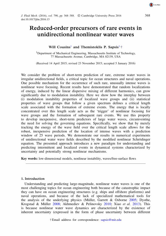
We consider the problem of short-term prediction of rare, extreme water waves inirregular unidirectional fields, a critical topic for ocean structures and naval operations.One possible mechanism for the occurrence of such rare, unusually intense waves isnonlinear wave focusing. Recent results have demonstrated that random localizationsof energy, induced by the linear dispersive mixing of different harmonics, can growsignificantly due to modulation instability. Here we show how the interplay between(i) modulation instability properties of localized wave groups and (ii) statisticalproperties of wave groups that follow a given spectrum defines a critical lengthscale associated with the formation of extreme events. The energy that is locallyconcentrated over this length scale acts as the ‘trigger’ of nonlinear focusing forwave groups and the formation of subsequent rare events. We use this propertyto develop inexpensive, short-term predictors of large water waves, circumventingthe need for solving the governing equations. Specifically, we show that by merelytracking the energy of the wave field over the critical length scale allows for therobust, inexpensive prediction of the location of intense waves with a predictionwindow of 25 wave periods. We demonstrate our results in numerical experimentsof unidirectional water wave fields described by the modified nonlinear Schrödingerequation. The presented approach introduces a new paradigm for understanding andpredicting intermittent and localized events in dynamical systems characterized byuncertainty and potentially strong nonlinear mechanisms.

Key words: low-dimensional models, nonlinear instability, waves/free-surface flows

1. IntroductionUnderstanding and predicting large-magnitude, nonlinear water waves is one of the

most challenging topics for ocean engineering both because of the catastrophic impactthey can have on ocean engineering structures (e.g. ships and offshore platforms) andnaval operations, and because of the lack of specialized mathematical tools forthe analysis of the underlying physics (Müller, Garrett & Osborne 2005; Dysthe,Krogstad & Müller 2008; Akhmediev & Pelinovsky 2010; Xiao et al. 2013). Thisis because nonlinear water wave dynamics are characterized by the existence ofinherent uncertainty (expressed in the form of phase uncertainty between different

† Email address for correspondence: [email protected]

mailto:[email protected]

http://crossmark.crossref.org/dialog/?doi=10.1017/jfm.2016.13&domain=pdf

Precursors of rare events in unidirectional nonlinear water waves 369

Fourier modes) and in the form of strong nonlinearities and associated energy transfersbetween modes. The latter can be activated locally and intermittently, leading tounusually high-magnitude waves that emerge out of the complex background wavefield.

An extreme form of such dynamical evolution is the case of freak or rogue waveswith wave height which can be as large as eight times the standard deviation ofthe surrounding wave field (Onorato et al. 2005; Dysthe et al. 2008). Waves of thismagnitude have caused considerable damage to ships, oil rigs and human life (Haver2004; Liu 2007). In addition, many naval operations, e.g. transfer of cargo betweenships moored together in a sea base, landing on aircraft carriers, or path planningof high-speed surface vehicles, require short-term prediction of the surrounding wavefield. To make such predictions, unusually high wave elevations must be forecastedreliably.

One mechanism for the occurrence of such rare, unusually intense wave elevationsis nonlinear wave focusing (Onorato, Osborne & Serio 2002a; Janssen 2003; Cousins& Sapsis 2015). For deep-water waves a manifestation of this focusing is thewell-known Benjamin–Feir (BF) instability of a plane wave to small sidebandperturbations. This instability, which has also been demonstrated experimentally(Chabchoub, Hoffmann & Akhmediev 2011), generates huge coherent structures bysoaking up energy from the nearby field (Benjamin & Feir 1967; Zakharov 1968;Osborne, Onorato & Serio 2000). Cousins & Sapsis (2015) demonstrated that evenimperfect background conditions, i.e. completely different from the idealized planewave set-up of the BF instability, can still lead to important wave focusing and rareevents. In particular, it was analytically shown and numerically demonstrated forunidirectional wavetrains that there is a critical combination of wave group lengthscales and amplitudes which will lead to wave focusing and thus unusually highelevations. In contrast to the standard BF mechanism, these instabilities are initiatedbecause of sufficiently large spatially localized energy.

Such energy localization, which can ‘trigger’ nonlinear wave focusing, can occuras the result of random relative phases between different harmonics. This phaserandomness is mainly introduced by the mixing of different harmonics due to theirlinear dispersive propagation. Thus, the linear propagation of water waves can locallycreate conditions that will lead to nonlinear focusing and subsequent rare events. Itis clear that this perspective provides a scenario in which the unstable extreme waveevents are isolated occurrences of strongly nonlinear focusing events initiated by thelinear or weakly nonlinear background.

Therefore, on the one hand we have the nonlinear wave mechanics that define whichlocalized wave groups will focus because of modulation instabilities, while on theother hand we have the power spectrum that defines what wave groups can formdue to random phase difference between harmonics. The scope of this work is tocombine these two perspectives in order to derive precursors of rare events that willtake into account not only the nonlinear mechanics of water waves (in particular themodulation instability) but also the spectral or statistical properties of the wave field.In particular, we show how the interplay between (i) modulation instability propertiesof localized wave groups and (ii) statistical properties of wave groups associated witha given spectrum defines a critical length scale that is related with the occurrence ofstrongly nonlinear interactions and the formation of extreme events. The energy that islocally concentrated over this length scale acts essentially as the ‘trigger’ of nonlinearfocusing of wave groups.

We use this property to derive short-term precursors for the occurrence of largewater waves, circumventing the need for solving the governing equations. To quantify

370 W. Cousins and T. P. Sapsis

the probability of occurrence of specific wave groups from a given spectrum we usea scale selection algorithm (Lindeberg 1998). This statistical analysis is combinedwith an analytical nonlinear stability criterion for focusing of localized wave groups(Cousins & Sapsis 2015) to yield a reliable, computationally inexpensive forecastof the subsequent growth for each wave group in the field. In a second stage, wedemonstrate that merely tracking the energy of the wave field over the critical lengthscale defined by the interplay between statistics and nonlinearity allows for an evencheaper and robust forecast of upcoming intense nonlinear wave elevations, with aprediction window of the order of 25 wave periods. We demonstrate our results innumerical experiments involving unidirectional water wave fields described by themodified nonlinear Schrödinger equation (MNLS).

Our proposed predictive method reveals and directly uses the low-dimensionalcharacter of the domain of attraction of these rare water waves. In particular,despite the distribution of the background energy over a wide range of scales,the ‘trigger’ of nonlinear focusing is essentially low-dimensional and to this endit can be used as an inexpensive way to estimate the probability for a rare eventin the near future. Our scheme is robust, performing well even with noise andirregularity in the wave field. Furthermore, the presented approach introduces a newparadigm for handling spatiotemporal rare events in dynamical systems with inherentuncertainty by providing an efficient description of the ‘trigger’ that leads to thoserare events through the careful study of the synergistic action between uncertaintyand nonlinearity.

We stress that our method differs significantly from previously described predictiveschemes. For example, the inverse scattering approach of Islas & Schober (2005)is, in its proposed form, limited to the nonlinear Schrödinger equation (NLS).Our wave-group-based scheme easily applies to the more accurate MNLS wheresuch analytical tools are not available. Also, our scheme is similar in spirit to thequasi-determinism (QD) theory of Boccotti (2008), which extends the observationthat profiles of large-amplitude waves resemble the autocorrelation function (Lindgren1970; Boccotti 1983). Boccotti’s QD theory is linear and has been extended toinclude second-order effects by Fedele & Tayfun (2009). Although second-orderQD agrees well with many oceanic observations, our scheme allows us to performprediction of rare events occurring due to nonlinear focusing effects induced bywave–wave interactions which are associated with highly nonlinear regimes wherecurrent analytical methods are limited.

2. Extreme events in envelope equationsIn this work, we consider irregular waves travelling on the surface of a fluid

of infinite depth. A typical approach for modelling this phenomenon is to assumeincompressible, irrotational, inviscid flow, which gives Laplace’s equation for thevelocity potential. This equation is paired with two boundary conditions on thesurface: a pressure condition and a kinematic one (a particle initially on the freesurface remains so). This model agrees well with laboratory experiments (Wu, Ma& Eatock Taylor 1998), and faithfully reproduces the classical k−5/2 spectral tailobserved in deep water (Onorato et al. 2002b). Although some care is required todeal numerically with the free surface, this fully nonlinear model may be solvednumerically with reasonable computational effort, particularly in one space dimension(Dommermuth & Yue 1987; Craig & Sulem 1993; Dyachenko et al. 1996; Choi &Camassa 1999). However, the presence of the free surface makes analysis of theunderlying dynamics challenging.


Here we consider approximate equations governing the evolution of the waveenvelope, the NLS (Zakharov 1968) and the MNLS of (Dysthe 1979). Both NLSand MNLS can be derived via a perturbation approach from the fully nonlinearmodel under assumptions of small steepness and slow variation of the wave envelope.Although forms of these equations exist in a full two-dimensional setting, here weconsider wave fields varying only in the direction of propagation. The NLS, innon-dimensionalized coordinates, reads

∂u∂t+ 1

2∂u∂x+ i

8∂2u∂x2+ i

2|u|2u= 0, (2.1)

where u(x, t) is the wave envelope. To leading order the surface elevation is given byη(x, t) = Re[u(x, t)ei(x−t)]. Equation (2.1) has been non-dimensionalized with x = k0x,t=ω0 t and u= k0u, where x, t and u are physical space, time and envelope, k0 is thedominant spatial frequency of the surface elevation and ω0 =√gk0.

Our primary interest in this work is the MNLS, which is a higher-order approxima-tion of the fully nonlinear model,

∂u∂t+ 1

2∂u∂x+ i

8∂2u∂x2− 1

16∂3u∂x3+ i

2|u|2u+ 3

2|u|2 ∂u

∂x+ 1

4u2 ∂u∗

∂x+ iu

∂φ

∂x

∣∣∣∣z=0

= 0, (2.2)

where φ is the velocity potential and ∂φ/∂x|z=0 = −F−1[|k|F [|u|2]]/2, and Fdenotes the Fourier transform. The MNLS has been shown to reproduce laboratoryexperiments reasonably well (Lo & Mei 1985; Goullet & Choi 2011). There areeven higher-order envelope equations, such as the broadband modified nonlinearSchrödinger equation (BMNLS) (Trulsen & Dysthe 1996) as well as the more recentcompact Zakharov equation (Dyachenko & Zakharov 2011). The latter is valid forthird-order nonlinearities and it does not have restrictions on the spectral bandwidth(Fedele 2014). However, we do not discuss these equations here. Although there areconsiderable differences between NLS and MNLS, we found minimal differencesbetween simulations of MNLS and BMNLS. Dysthe et al. (2003) also found similaragreement between MNLS and BMNLS.

These envelope equations, as well as the fully nonlinear water wave model,admit periodic plane wave solutions. Interestingly, these plane wave solutions areunstable to sideband perturbations (Benjamin & Feir 1967; see also Zakharov 1968),a phenomenon termed the BF instability. This instability has a striking manifestation.Energy is ‘sucked up’ from the nearby field to produce a large-amplitude coherentstructure, containing a wave 2.4–3 times larger than the surrounding backgroundfield (Osborne et al. 2000). This behaviour has been shown numerically in envelopeequations (Yuen & Fergusen 1978; Dysthe & Trulsen 1999) as well as in the fullynonlinear formulation (Henderson, Peregrine & Dold 1999). Furthermore, a numberof experiments confirm these numerical predictions (Chabchoub et al. 2011, 2012).

However, in realistic physical settings, the water surface is not merely a plane wave– energy is distributed over a range of frequencies. To this end, we consider extremewaves emerging out of a background with Gaussian spectra and random phases,that is

u(x, 0)=N/2∑−N/2+1

√2∆kF(k∆k) ei(ωkx+ξk), F(k)= ε2

σ√

2πe−k2/2σ 2

, (2.3a,b)


Surf

ace

elev

atio

n

Space

(a) (b)

Space

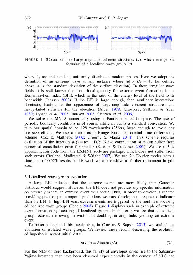
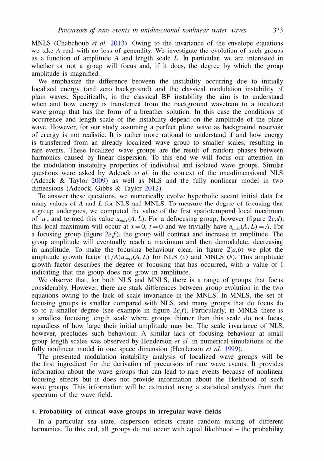
FIGURE 1. (Colour online) Large-amplitude coherent structures (b), which emerge viafocusing of a localized wave group (a).

where ξk are independent, uniformly distributed random phases. Here we adopt thedefinition of an extreme wave as any instance where |u| > HE = 4ε (as definedabove, ε is the standard deviation of the surface elevation). In these irregular wavefields, it is well known that the critical quantity for extreme event formation is theBenjamin–Feir index (BFI), which is the ratio of the energy level of the field to itsbandwidth (Janssen 2003). If the BFI is large enough, then nonlinear interactionsdominate, leading to the appearance of large-amplitude coherent structures andheavy-tailed statistics for the elevation (Alber 1978; Crawford, Saffman & Yuen1980; Dysthe et al. 2003; Janssen 2003; Onorato et al. 2005).

We solve the MNLS numerically using a Fourier method in space. The use ofperiodic boundary conditions is of course artificial, but is a standard convention. Wetake our spatial domain to be 128 wavelengths (256π), large enough to avoid anybox-size effects. We use a fourth-order Runge–Kutta exponential time differencingscheme (Cox & Matthews 2002; Grooms & Majda 2014). This scheme requiresevaluation of the function φ(z)= (ez − 1)/z. Naive computation of φ can suffer fromnumerical cancellation error for small z (Kassam & Trefethen 2005). We use a Padéapproximation code from the EXPINT software package, which does not suffer fromsuch errors (Berland, Skaflestad & Wright 2007). We use 210 Fourier modes with atime step of 0.025; results in this work were insensitive to further refinement in gridsize.

3. Localized wave group evolutionA large BFI indicates that the extreme events are more likely than Gaussian

statistics would suggest. However, the BFI does not provide any specific informationon precisely where an extreme event will occur. Thus, in order to develop a schemeproviding precise spatiotemporal predictions we must develop a more precise indicatorthan the BFI. In high-BFI seas, extreme events are triggered by the nonlinear focusingof localized wave groups (Fedele 2008). Figure 1 displays such an example of extremeevent formation by focusing of localized groups. In this case we see that a localizedgroup focuses, narrowing in width and doubling in amplitude, yielding an extremeevent.

To better understand this mechanism, in Cousins & Sapsis (2015) we studied theevolution of isolated wave groups. We review these results describing the evolutionof hyperbolic secant initial data:

u(x, 0)= A sech(x/L). (3.1)

For the NLS on zero background, this family of envelopes gives rise to the Satsuma–Yajima breathers that have been observed experimentally in the context of NLS and


MNLS (Chabchoub et al. 2013). Owing to the invariance of the envelope equationswe take A real with no loss of generality. We investigate the evolution of such groupsas a function of amplitude A and length scale L. In particular, we are interested inwhether or not a group will focus and, if it does, the degree by which the groupamplitude is magnified.

We emphasize the difference between the instability occurring due to initiallylocalized energy (and zero background) and the classical modulation instability ofplain waves. Specifically, in the classical BF instability the aim is to understandwhen and how energy is transferred from the background wavetrain to a localizedwave group that has the form of a breather solution. In this case the conditions ofoccurrence and length scale of the instability depend on the amplitude of the planewave. However, for our study assuming a perfect plane wave as background reservoirof energy is not realistic. It is rather more rational to understand if and how energyis transferred from an already localized wave group to smaller scales, resulting inrare events. These localized wave groups are the result of random phases betweenharmonics caused by linear dispersion. To this end we will focus our attention onthe modulation instability properties of individual and isolated wave groups. Similarquestions were asked by Adcock et al. in the context of the one-dimensional NLS(Adcock & Taylor 2009) as well as NLS and the fully nonlinear model in twodimensions (Adcock, Gibbs & Taylor 2012).

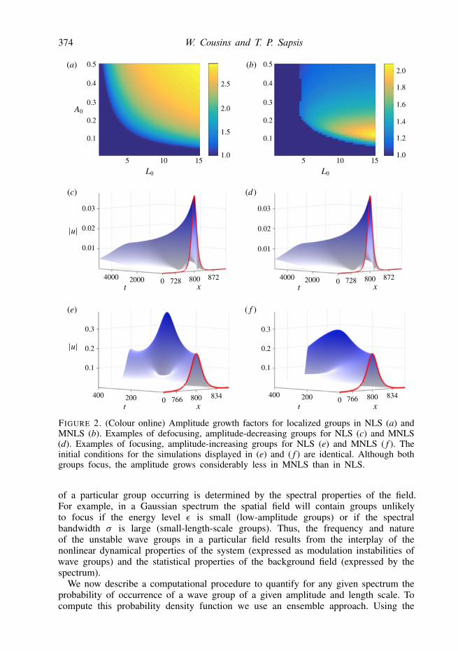
To answer these questions, we numerically evolve hyperbolic secant initial data formany values of A and L for NLS and MNLS. To measure the degree of focusing thata group undergoes, we computed the value of the first spatiotemporal local maximumof |u|, and termed this value umax(A,L). For a defocusing group, however (figure 2c,d),this local maximum will occur at x= 0, t= 0 and we trivially have umax(A,L)=A. Fora focusing group (figure 2e,f ), the group will contract and increase in amplitude. Thegroup amplitude will eventually reach a maximum and then demodulate, decreasingin amplitude. To make the focusing behaviour clear, in figure 2(a,b) we plot theamplitude growth factor (1/A)umax(A, L) for NLS (a) and MNLS (b). This amplitudegrowth factor describes the degree of focusing that has occurred, with a value of 1indicating that the group does not grow in amplitude.

We observe that, for both NLS and MNLS, there is a range of groups that focusconsiderably. However, there are stark differences between group evolution in the twoequations owing to the lack of scale invariance in the MNLS. In MNLS, the set offocusing groups is smaller compared with NLS, and many groups that do focus doso to a smaller degree (see example in figure 2e,f ). Particularly, in MNLS there isa smallest focusing length scale where groups thinner than this scale do not focus,regardless of how large their initial amplitude may be. The scale invariance of NLS,however, precludes such behaviour. A similar lack of focusing behaviour at smallgroup length scales was observed by Henderson et al. in numerical simulations of thefully nonlinear model in one space dimension (Henderson et al. 1999).

The presented modulation instability analysis of localized wave groups will bethe first ingredient for the derivation of precursors of rare wave events. It providesinformation about the wave groups that can lead to rare events because of nonlinearfocusing effects but it does not provide information about the likelihood of suchwave groups. This information will be extracted using a statistical analysis from thespectrum of the wave field.

4. Probability of critical wave groups in irregular wave fieldsIn a particular sea state, dispersion effects create random mixing of different

harmonics. To this end, all groups do not occur with equal likelihood – the probability


0.5(a)

(c)

(e)

(d )

( f )

(b)

2.5

2.0

1.5

1.05 10 15

0.4

0.3

0.2

0.1

0.52.0

1.8

1.6

1.4

1.2

1.0

0.4

0.3

0.2

0.1

5 10 15

0.03

4000 2000 0 728 800 872

0.02

0.01

0.03

0.02

0.01

4000 2000 0 728 800 872

0.3

0.2

0.1

400 200 0 766 800 834

0.3

0.2

0.1

400 200 0 766 800 834

FIGURE 2. (Colour online) Amplitude growth factors for localized groups in NLS (a) andMNLS (b). Examples of defocusing, amplitude-decreasing groups for NLS (c) and MNLS(d). Examples of focusing, amplitude-increasing groups for NLS (e) and MNLS ( f ). Theinitial conditions for the simulations displayed in (e) and ( f ) are identical. Although bothgroups focus, the amplitude grows considerably less in MNLS than in NLS.

of a particular group occurring is determined by the spectral properties of the field.For example, in a Gaussian spectrum the spatial field will contain groups unlikelyto focus if the energy level ε is small (low-amplitude groups) or if the spectralbandwidth σ is large (small-length-scale groups). Thus, the frequency and natureof the unstable wave groups in a particular field results from the interplay of thenonlinear dynamical properties of the system (expressed as modulation instabilities ofwave groups) and the statistical properties of the background field (expressed by thespectrum).

We now describe a computational procedure to quantify for any given spectrum theprobability of occurrence of a wave group of a given amplitude and length scale. Tocompute this probability density function we use an ensemble approach. Using the


0 5 10 15 20

0.05

0.10

0.15

0.20

0.25

5 10 15 20 25 30

PDF

valu

ePD

F va

lue

0

0.02

0.04

0.06

0.08

0.10

0.12

0.14NLSMNLS

2 4 6 8 100

0.1

0.2

0.3

0.4

0.5

0 5 10 15 20

0.05

0.10

0.15

0.20

0.25

0.14(a)

(b) (c)

(d) (e)

0.12

0.01

0.08

0.06

0.04

0.02

0 100 200 300 400 500 600 700 800

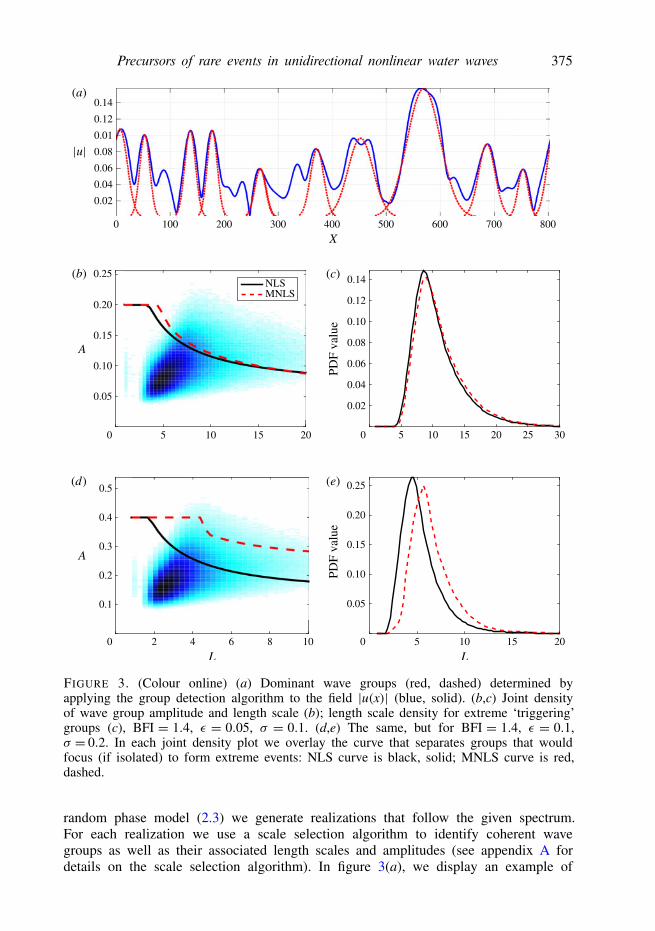
FIGURE 3. (Colour online) (a) Dominant wave groups (red, dashed) determined byapplying the group detection algorithm to the field |u(x)| (blue, solid). (b,c) Joint densityof wave group amplitude and length scale (b); length scale density for extreme ‘triggering’groups (c), BFI = 1.4, ε = 0.05, σ = 0.1. (d,e) The same, but for BFI = 1.4, ε = 0.1,σ = 0.2. In each joint density plot we overlay the curve that separates groups that wouldfocus (if isolated) to form extreme events: NLS curve is black, solid; MNLS curve is red,dashed.

random phase model (2.3) we generate realizations that follow the given spectrum.For each realization we use a scale selection algorithm to identify coherent wavegroups as well as their associated length scales and amplitudes (see appendix A fordetails on the scale selection algorithm). In figure 3(a), we display an example of


such a random realization field |u(x)| as well as the groups identified by the groupdetection algorithm, showing that this algorithm appropriately picks out the dominantgroups. We then compute the joint probability density of group amplitude and lengthscale by applying this group identification algorithm to 50 000 realizations of Gaussianspectrum random fields.

The described step has very low computational cost since it does not involvethe numerical solution of dynamical equations but only the statistical analysisof wave realizations that follow a given spectrum. It is the second ingredient,the statistical component of our analysis, which we will now combine with themodulation instability analysis of localized wave groups presented in the previoussection. More specifically, using the analysis for the evolution of localized wavegroups, we determine, for each length scale L, the smallest group amplitude requiredto ‘trigger’ an extreme event. That is, if the extreme event threshold is HE = 4ε, wefind, for each L, the smallest A such that umax(A, L)>HE. Denoting this amplitude asA∗, we trivially have A∗6HE. This procedure describes a curve A∗(L), where isolatedgroups located above this curve in the (L, A) plane would yield an extreme event,and those below this curve would not. Note that wave groups with sufficiently smallinitial length scales L will never undergo nonlinear focusing. For these length scalesthe only wave groups that can reach amplitudes as large as HE are the ones that startwith A∗(L)=HE. This observation explains the plateau that occurs for small L.

In figure 3 we overlay this curve (which expresses dynamical properties of nonlinearwave groups) over the joint density of group amplitude and length scale (whichexpresses statistical properties of the wave spectrum). For a given spectrum, we maydetermine the frequency and nature of extreme event triggering groups (i.e. thoselying above the respective curves in figure 3). As expected, increasing the energylevel or decreasing the spectral bandwidth increases the number of these extremetriggering groups. This analysis provides a concrete, wave-group-based explanationof the development of heavy tails via nonlinear interactions in high-BFI regimes.However, unlike traditional BFI-based analysis, this wave group analysis directlyincorporates the lack of scale invariance in MNLS. This is clear from figure 3(b–e)where we display (A, L) densities for two different spectra with the same BFI. Wenote the scale invariance property of NLS (note that the two black curves are identical,albeit the axes rescale) and how this contrasts with the corresponding curves (reddashed lines) for the MNLS, which change between the two spectra even though theBFI index remains the same.

The main benefit of this statistical instability analysis allows us to characterizethe properties of extreme event triggering groups in a maximum likelihood sense.Specifically, for a given spectrum, we can compute the density of the length scaleof groups that would generate extreme events (i.e. those lying above the curves offigure 3b,d). In figure 3(c,e) we display examples of these length scale densities forthe two different spectra. The concentration of these densities around their peak valuesuggests that for a given spectrum there is a most likely extreme event triggeringlength scale, LE. As the distribution is fairly narrow, we expect that the majority ofextreme events that occur will be triggered by localization at length scales close toLE. In § 5, we will use this fact to develop a predictive scheme based on projectingthe field onto an appropriately tuned set of Gabor wavelets.

5. Precursors of extreme eventsIn this section, we describe the central result of this paper, which is the derivation of

precursors for extreme events in nonlinear water waves. These precursors allow for the


detection of instabilities at their very early stages and therefore lead to the predictionof rare events without the need to solve the full envelope equations.

We describe two precursor forms. First, we develop an algorithm to predict extremeevents by identifying the dominant wave groups in a given field, and use our resultsfrom § 3 regarding localized groups that can ‘trigger’ an extreme event. Second, wedevelop a scheme based on projecting the field onto a carefully tuned set of Gabormodes. We find that large values of a certain Gabor coefficient indicate that anupcoming extreme event is likely. This Gabor-based scheme is nearly as reliable asthe group detection scheme, yet requires a remarkably smaller computational cost.

5.1. Prediction by wave group identificationHere we describe a straightforward scheme for advance prediction of extreme eventsvia wave group identification. For a given wave field, we apply the group identificationalgorithm described in appendix A to the envelope. This gives the spatial location,amplitude A and length scale L of each wave group. We then predict the futurefocused amplitude of the group by evaluating umax(A,L), where umax is the numericallyconstructed function from our prior study of localized groups in § 3. If umax(A,L) is atleast 95 % of the extreme event threshold HE, then we predict that an extreme eventwill occur. We choose this conservative prediction threshold in order to minimize thenumber of false negatives (extreme events that we fail to predict).

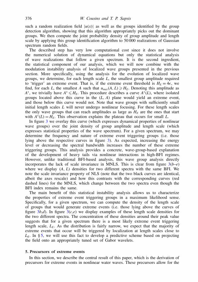
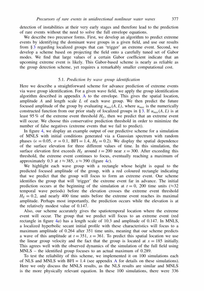
In figure 4, we display an example output of our predictive scheme for a simulationof MNLS with initial conditions generated via a Gaussian spectrum with randomphases (ε = 0.05, σ = 0.1, BFI = 1.4, HE = 0.2). We display the spatial dependenceof the surface elevation for three different values of time. In this simulation, thesurface elevation first exceeds HE around t = 200 near x= 300. After exceeding thisthreshold, the extreme event continues to focus, eventually reaching a maximum ofapproximately 0.3 at t≈ 385, x≈ 390 (figure 4c).

We highlight each wave group with a rectangle whose height is equal to thepredicted focused amplitude of the group, with a red coloured rectangle indicatingthat we predict that the group will focus to form an extreme event. Our schemeidentifies the group that will ‘trigger’ the extreme event far in advance. The initialprediction occurs at the beginning of the simulation at t = 0, 200 time units (≈32temporal wave periods) before the elevation crosses the extreme event thresholdHE = 0.2, and nearly 400 time units before the extreme event reaches its maximalamplitude. Perhaps most importantly, the prediction occurs while the elevation is atthe relatively modest value of 0.147.

Also, our scheme accurately gives the spatiotemporal location where the extremeevent will occur. The group that we predict will focus to an extreme event (redrectangle in figure 4a) has a length scale of 10.3 and amplitude of 0.147. In MNLS,a localized hyperbolic secant initial profile with these characteristics will focus to amaximum amplitude of 0.264 after 351 time units, meaning that our scheme predictsa wave of this amplitude at t= 351, x= 361. To predict this spatial location we usethe linear group velocity and the fact that the group is located at x = 185 initially.This agrees well with the observed dynamics of the simulation of the full field usingMNLS – the identified group focuses to an actual maximum of 0.289.

To test the reliability of this scheme, we implemented it on 100 simulations eachof NLS and MNLS with BFI = 1.4 (see appendix A for details on these simulations).Here we only discuss the MNLS results, as the NLS results are similar and MNLSis the more physically relevant equation. In these 100 simulations, there were 336


0.2(a)

(b)

(c)

Surf

ace

elev

atio

n0.1

0

–0.1

–0.2

–0.3

0.2

Surf

ace

elev

atio

n

0.1

0

–0.1

–0.2

–0.3

0.2

Surf

ace

elev

atio

n

0.1

0

–0.1

–0.2

–0.3

0 50 100 150 200 250 300 350 400 450 500

0 50 100 150 200 250 300 350 400 450 500

0 50 100 150 200 250 300 350 400 450 500

Space

FIGURE 4. (Colour online) (a) Initial conditions for a simulation of MNLS, t = 0. Ourscheme identifies a group around x = 190 which we predict will grow to form a largeextreme event. (b) Group in initial stages of focusing, t= 202.5, which breaks the extremeevent threshold HE = 0.2 near x= 290. (c) Group is fully focused, t= 384.5, and attainsits maximum amplitude near x= 390.

extreme events. We predicted all of these extreme events in advance – there were nofalse negatives. There were 91 instances where we predicted an extreme event but onedid not occur, giving a false positive rate of 21.3 %. For our correct predictions, theaverage warning time (the amount of time before the prediction began and the onsetof the extreme event) was 153 time units (≈24 temporal wave periods).

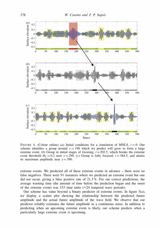
Our scheme has value beyond a binary predictor of extreme events. In figure 5(a),we display a scatter plot showing the relationship between the predicted futureamplitude and the actual future amplitude of the wave field. We observe that ourpredictor reliably estimates the future amplitude in a continuous sense. In addition topredicting when an upcoming extreme event is likely, our scheme predicts when aparticularly large extreme event is upcoming.


0.4(a)

(b)

0.25

0.20

0.15

0.10

0.05

0.3

0.2

Act

ual a

mpl

itude

0.1

0.1 0.2

Predicted amplitude0.3 0.4 160 180 200 220 240 0

200400

FIGURE 5. (Colour online) (a) Scatter plot of predicted versus actual amplitudes as wellas the line predicted = actual (red). Note that the vertical dashed line is located at 0.95HEto reduce false negatives (as discussed in the text). (b) Spatiotemporal dependence of |u|(red) and predicted future amplitude (blue).

To further illustrate the skill of our scheme, in figure 5(b), we plot the surface|u(x, t)| in red, as well as the predicted future group shape in blue. The field displayedhere is the same field displayed in figure 4 in a coordinate frame moving with thelinear group velocity. The surface plots in figure 5 provide a visualization of the skillof our scheme in predicting the future amplitude of the extreme wave, as well as thespatial location at which it will occur. The blue surface near the extreme event decaysand vanishes around t=200 because we locally turn off the predictor while an extremeevent is occurring (|u|>HE).

5.2. Prediction by Gabor projection

We now describe an alternative reliable prediction scheme that requires negligiblecomputational cost. In this scheme, we predict upcoming extreme events by projectingthe field onto a set of carefully tuned Gabor modes. This approach is similar in spiritto our extreme event predictive scheme for the model of Majda, McLaughlin andTabak (MMT) (Cousins & Sapsis 2014). This projection requires only a singleconvolution integral, so its computation is extremely cheap. Even at this low cost,this scheme reliably predicts upcoming extreme events with spatiotemporal skill.

As we showed in § 3, for a given spectrum we can compute the joint density ofwave group amplitude and length scale. Using our study of isolated localized groups,we can then compute the conditional density of wave group properties for groupsthat will ‘trigger’ extreme events. This gives the density of group length scalesfor groups that would focus to form an extreme event (refer to figure 3c,e). Fromthis, we can compute the spatial length scale LG with the maximum likelihood of‘triggering’ an extreme event. Owing to the narrowness of the distribution of extremeevent triggering group length scales, we expect that extreme events will be precededby energy localization at a length scale close to LG.

To predict extreme events, we estimate the energy concentrated in scale LG.To do so, we ‘project’ the field onto the set of Gabor basis functions vn(x; xc),


0.25(a) (b) 1.0

0.8

0.6

0.4

0.2

0 0.1 0.2 0.3 0.4 0 0.05 0.10 0.15 0.20

0.20

0.15

0.10

0.05

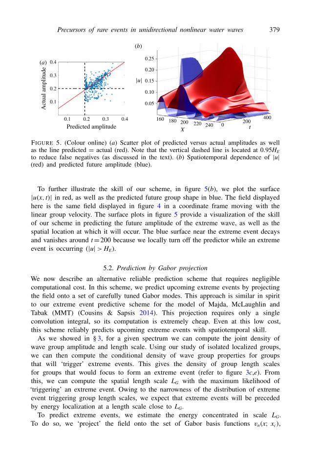
FIGURE 6. (Colour online) (a) Family of conditional densities of current |Y0| and future|u|, corresponding to (5.3). (b) Probability of upcoming extreme event as a functionof |Y0|.

complex exponentials multiplied by a Gaussian window function. This gives theGabor coefficients Yn(xc, t):

vn(x; xc)= eiπn(x−xC)/LGe−(x−xC)2/2L2

G, (5.1)Yn(xc, t)= 〈u(x, t), vn(x; xc)〉/〈vn(x; xc), vn(x; xc)〉. (5.2)

We claim that a large value of Y0 at a spatial point xc indicates that an extreme eventis likely in the future near xc in space (in a frame moving with the group velocity).To confirm this, we compute the following family of conditional distributions.

FY0(U ),P

max|x∗−xc|<LG

t∗∈[t+tA,t+tB]|u(x∗, t∗)|>U

∣∣∣∣ |Y0(xc, t)| =Y0

. (5.3)

That is, given a particular current value of Y0, we examine what are the statistics ofthe envelope u in the future. Here we choose tA = 50 and tB = 350 from the timerequired for a group of length scale of LG to focus to form an extreme event. Wecompute the statistics (5.3) from 200 simulations of NLS/MNLS with Gaussian spectraand random phases with ε = 0.05, σ = 0.1 and BFI= 1.4.

In figure 6(a), we display the family of conditional densities of future |u| for arange of values of |Y0|. These densities show that, when |Y0| is large, |u| is essentiallyguaranteed to be large in the future. From these conditional statistics, we computethe probability of an upcoming extreme event PEE as a function of current Y0 byintegrating over (HE,∞). This function is displayed in figure 6(b). Probability PEEhas a sigmoidal dependence on Y0: if Y0 is large enough then an upcoming extremeevent is nearly guaranteed, while if Y0 is small enough then an upcoming extremeevent is highly unlikely.

Our predictor Y0 becomes large distinctly before the extreme event occurs. Theconditional statistics shown in figure 6 pair a value of Y0 with a maximum value of |u|which occurs at least tA = 50 time units in the future. To further illustrate this point,we statistically investigate the energy exchanges between the various Gabor modes. Todo so, we compute the statistics of the Gabor coefficients during, before and far froman extreme event. We display these Gabor statistics in figure 7. We see that, awayfrom extreme events, we have nearly Gaussian statistics for the coefficients. In this


0.04

(a)

(d) (e) ( f )

(b) (c)

0.030.020.01

0.01

00

50

–5–10–15

0.01

0

–0.01

–0.01 –0.01

–0.02–0.03–0.04

0.05

0.05

0

0

–0.05 –0.05

0.1 0.10.2

0.05

–0.0500 0

–0.1 –0.1

Con

d. P

DF

valu

e

25

20

15

10

5

0 0.1 0.2

DuringBeforeFar from

0.3

60

40

20

0 0.05 0.10

100

80

60

40

20

0 0.02 0.04 0.06 0.08 0.10

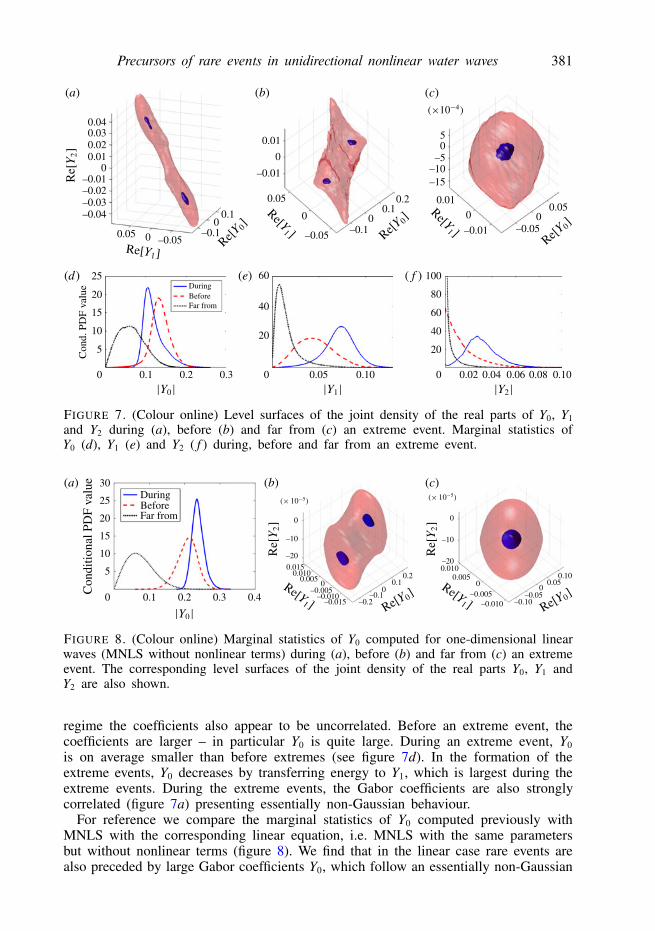
FIGURE 7. (Colour online) Level surfaces of the joint density of the real parts of Y0, Y1and Y2 during (a), before (b) and far from (c) an extreme event. Marginal statistics ofY0 (d), Y1 (e) and Y2 ( f ) during, before and far from an extreme event.

0 0.1 0.2 0.3 0.4

5

10

15

20

DuringBeforeFar from 0

–10

–20

0.0150.010

0.0050

–0.005–0.010

–0.015 –0.2–0.1

00.1

0.2

0

–10

–200.010

0.0050

–0.005–0.010 –0.10

–0.050

0.050.10

Con

ditio

nal P

DF

valu

e

25

30(a) (b) (c)

FIGURE 8. (Colour online) Marginal statistics of Y0 computed for one-dimensional linearwaves (MNLS without nonlinear terms) during (a), before (b) and far from (c) an extremeevent. The corresponding level surfaces of the joint density of the real parts Y0, Y1 andY2 are also shown.

regime the coefficients also appear to be uncorrelated. Before an extreme event, thecoefficients are larger – in particular Y0 is quite large. During an extreme event, Y0is on average smaller than before extremes (see figure 7d). In the formation of theextreme events, Y0 decreases by transferring energy to Y1, which is largest during theextreme events. During the extreme events, the Gabor coefficients are also stronglycorrelated (figure 7a) presenting essentially non-Gaussian behaviour.

For reference we compare the marginal statistics of Y0 computed previously withMNLS with the corresponding linear equation, i.e. MNLS with the same parametersbut without nonlinear terms (figure 8). We find that in the linear case rare events arealso preceded by large Gabor coefficients Y0, which follow an essentially non-Gaussian


–0.2

0 50

(a)

100 150 200 250 300 350 400 450 500

0

1

0

Surf

ace

elev

atio

n 0.2

0 50 100 150 200 250 300 350 400 450 500

0

0.5

1.0

0

Surf

ace

elev

atio

n

0 50 100 150 200 250 300 350 400 450 500

0

1

0

Surf

ace

elev

atio

n

Space

(b)

(c)

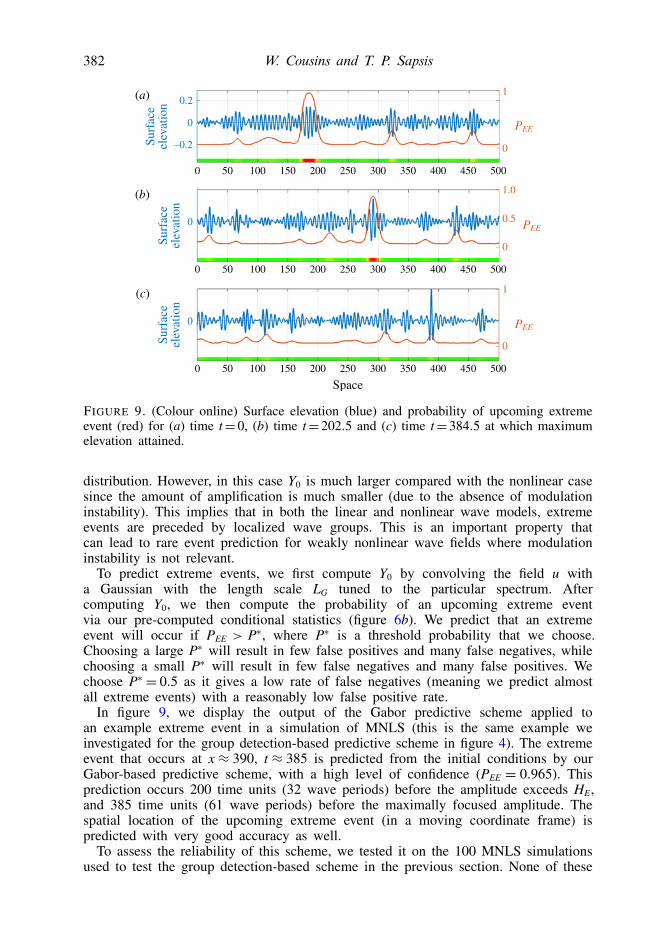
FIGURE 9. (Colour online) Surface elevation (blue) and probability of upcoming extremeevent (red) for (a) time t= 0, (b) time t= 202.5 and (c) time t= 384.5 at which maximumelevation attained.

distribution. However, in this case Y0 is much larger compared with the nonlinear casesince the amount of amplification is much smaller (due to the absence of modulationinstability). This implies that in both the linear and nonlinear wave models, extremeevents are preceded by localized wave groups. This is an important property thatcan lead to rare event prediction for weakly nonlinear wave fields where modulationinstability is not relevant.

To predict extreme events, we first compute Y0 by convolving the field u witha Gaussian with the length scale LG tuned to the particular spectrum. Aftercomputing Y0, we then compute the probability of an upcoming extreme eventvia our pre-computed conditional statistics (figure 6b). We predict that an extremeevent will occur if PEE > P∗, where P∗ is a threshold probability that we choose.Choosing a large P∗ will result in few false positives and many false negatives, whilechoosing a small P∗ will result in few false negatives and many false positives. Wechoose P∗ = 0.5 as it gives a low rate of false negatives (meaning we predict almostall extreme events) with a reasonably low false positive rate.

In figure 9, we display the output of the Gabor predictive scheme applied toan example extreme event in a simulation of MNLS (this is the same example weinvestigated for the group detection-based predictive scheme in figure 4). The extremeevent that occurs at x ≈ 390, t ≈ 385 is predicted from the initial conditions by ourGabor-based predictive scheme, with a high level of confidence (PEE = 0.965). Thisprediction occurs 200 time units (32 wave periods) before the amplitude exceeds HE,and 385 time units (61 wave periods) before the maximally focused amplitude. Thespatial location of the upcoming extreme event (in a moving coordinate frame) ispredicted with very good accuracy as well.

To assess the reliability of this scheme, we tested it on the 100 MNLS simulationsused to test the group detection-based scheme in the previous section. None of these


Predictive Extreme False False Averagescheme events negative positive warning time

Gaussian spectrum (ε = 0.05, σ = 0.1)

Gabor 336 20 (5.9 %) 108 (25.5 %) 245 (39 periods)Group detection 336 0 91 (21.3 %) 153 (24 periods)

Gaussian spectrum (ε = 0.05, σ = 0.2)

Gabor 342 29 (8.5 %) 121 (26.1 %) 193 (31 periods)Group detection 342 7 (2.0 %) 111 (24.5 %) 74 (12 periods)

JONSWAP spectrum

Gabor 383 7 (1.8 %) 139 (27.0 %) 237 (38 periods)Group detection 383 14 (3.7 %) 115 (23.1 %) 70 (11 periods)

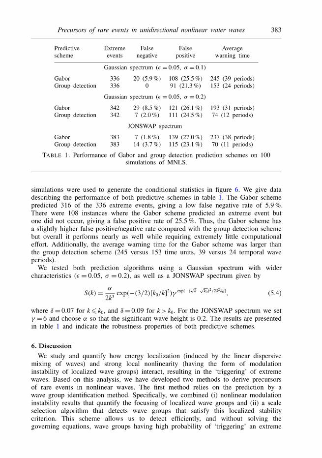
TABLE 1. Performance of Gabor and group detection prediction schemes on 100simulations of MNLS.

simulations were used to generate the conditional statistics in figure 6. We give datadescribing the performance of both predictive schemes in table 1. The Gabor schemepredicted 316 of the 336 extreme events, giving a low false negative rate of 5.9 %.There were 108 instances where the Gabor scheme predicted an extreme event butone did not occur, giving a false positive rate of 25.5 %. Thus, the Gabor scheme hasa slightly higher false positive/negative rate compared with the group detection schemebut overall it performs nearly as well while requiring extremely little computationaleffort. Additionally, the average warning time for the Gabor scheme was larger thanthe group detection scheme (245 versus 153 time units, 39 versus 24 temporal waveperiods).

We tested both prediction algorithms using a Gaussian spectrum with widercharacteristics (ε = 0.05, σ = 0.2), as well as a JONSWAP spectrum given by

S(k)= α

2k3exp(−(3/2)[k0/k]2)γ exp[−(√k−√k0)

2/2δ2k0], (5.4)

where δ= 0.07 for k6 k0, and δ= 0.09 for k> k0. For the JONSWAP spectrum we setγ =6 and choose α so that the significant wave height is 0.2. The results are presentedin table 1 and indicate the robustness properties of both predictive schemes.

6. DiscussionWe study and quantify how energy localization (induced by the linear dispersive

mixing of waves) and strong local nonlinearity (having the form of modulationinstability of localized wave groups) interact, resulting in the ‘triggering’ of extremewaves. Based on this analysis, we have developed two methods to derive precursorsof rare events in nonlinear waves. The first method relies on the prediction by awave group identification method. Specifically, we combined (i) nonlinear modulationinstability results that quantify the focusing of localized wave groups and (ii) a scaleselection algorithm that detects wave groups that satisfy this localized stabilitycriterion. This scheme allows us to detect efficiently, and without solving thegoverning equations, wave groups having high probability of ‘triggering’ an extreme


wave. Most importantly, the developed precursor can foresee an extreme event beforethe amplitude of the wave field becomes important.

The second method relies on the tracking of energy localized over a critical lengthscale. We used the scale selection algorithm to quantify, for a given wave spectrum,the probability of the formation of critical wave groups that can evolve into rareevents. This analysis revealed a spatial length scale where important energy has thehighest likelihood to ‘trigger’ a rare event. Based on this result, we formulated an evensimpler predictor relying on the Gabor transform, which locally tracks the energy ofthe wave field over the critical length scale. We applied the two predictive schemes inthe MNLS to forecast rare events in directional water waves. Both precursors reliablypredicted rogues in advance. Most importantly, this prediction was robust against noisein the background field, allowing for reliable forecast of, on average, 12–39 waveperiods before the occurrence of an extreme wave, depending on the initial spectrum.

Note that, although we considered (for demonstration purposes) unidirectionaldeep-water waves, where heavy tails are more prominent, there are no constraintsfor the presented theory to be applied in other set-ups involving the occurrence ofrare events due to dynamical instabilities. Indeed, heavy-tailed statistics is not a strictrequirement for our scheme. The presented approach introduces a new paradigmfor understanding and inexpensively predicting intermittent and localized events ingeneral dynamical systems where we have an interplay between uncertainty andnonlinearity. For such systems previous analytical studies have mainly focused on thequantification aspects of rare event statistics through the use of a generalized Paretodistribution (see e.g. Lucarini, Faranda & Wouters 2012; Lucarini et al. 2014). Asour approach uses minimal analytical tools, we believe it may be utilized for bothprediction and statistical quantification in settings where the dynamics are exceedinglycomplicated or entirely unknown (requiring a data-driven approach).

In the future, we plan to examine precursors of rare events for two-dimensionalwater waves, waves in regions with variable bathymetry, as well as waves in crossingseas. Deriving inexpensive precursors of strongly nonlinear instabilities will allowfor the improvement of direct numerical methods (see e.g. Alam 2014; Clausset al. 2014) for short-term prediction of the wave field evolution through the useof adaptive resolution techniques. To this end, we plan to combine the presentedprecursors with existing prediction schemes formulated for linear and weakly nonlinearequations in order to improve their efficiency by placing more computational effortin spatiotemporal regimes where strongly nonlinear interactions are expected.

AcknowledgementsThis research has been partially supported by the Naval Engineering Education

Center (NEEC) grant 3002883706 and by the Office of Naval Research (ONR) grantONR N00014-14-1-0520. The authors thank A. Chabchoub, F. Fedele, P. Gremaudand C. Merrill (NEEC Technical Point of Contact) for stimulating discussions. Theyalso thank the anonymous referees for numerous comments and suggestions that ledto important improvements.

Appendix A. Scale selection algorithmHere we describe the wave group detection algorithm used in the prediction scheme

discussed in § 5.1. To find the dominant wave groups in a given irregular wave field,we look for Gaussian-like ‘blobs’ in |u(x)|. To find these blobs, we use an existingalgorithm based on the scale-normalized derivatives of |u| (Koenderink 1984; Witkin


1984; Lindeberg 1998). These scale-normalized derivatives, s(m), are normalized spatialderivatives of the convolution of |u| with the heat kernel,

s(m)(x, L)= Lm/2 ∂m

∂xm( f ∗ g), (A 1)

where g(x, L) is the heat kernel,

g(x, L)= 1√2πL

e−x2/2L. (A 2)

In the above, x is the spatial variable and L is the length scale variable. FollowingLindeberg (1998) we choose m= 2 for optimal blob detection.

We illustrate this approach by computing the scale-normalized derivatives of a singleGaussian: u(x)=Ae−x2/2L2

0 . It is straightforward to show that s(2) has a local minimumat x=0, L=2L2

0. In an arbitrary field |u|, we similarly find wave groups by computings(2) and subsequently find the local minima. If we find a local minima at (xC, L∗),we conclude that there is a wave group at x= xC having a length scale

√L∗/2. We

determine the amplitude of the wave group, A, by computing the local maxima of |u|near xC.

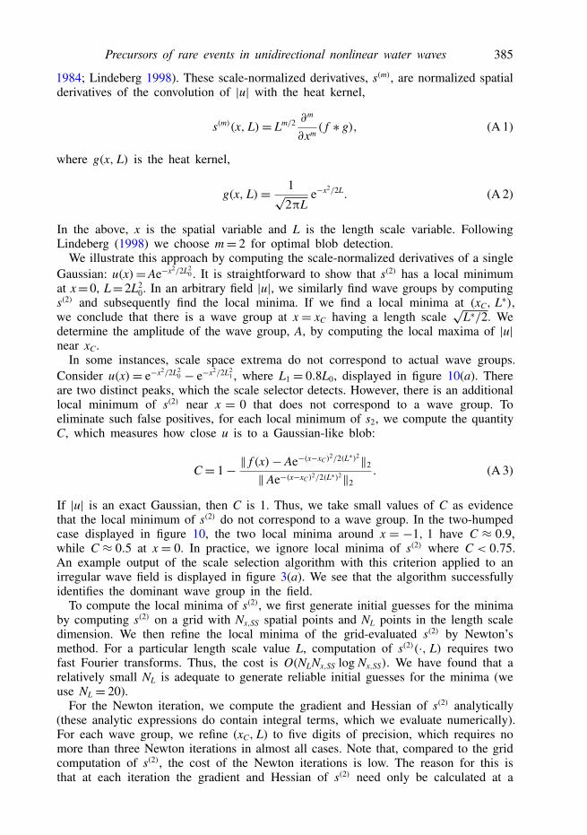
In some instances, scale space extrema do not correspond to actual wave groups.Consider u(x)= e−x2/2L2

0 − e−x2/2L21 , where L1 = 0.8L0, displayed in figure 10(a). There

are two distinct peaks, which the scale selector detects. However, there is an additionallocal minimum of s(2) near x = 0 that does not correspond to a wave group. Toeliminate such false positives, for each local minimum of s2, we compute the quantityC, which measures how close u is to a Gaussian-like blob:

C= 1− ‖ f (x)− Ae−(x−xC)2/2(L∗)2‖2

‖ Ae−(x−xC)2/2(L∗)2‖2. (A 3)

If |u| is an exact Gaussian, then C is 1. Thus, we take small values of C as evidencethat the local minimum of s(2) do not correspond to a wave group. In the two-humpedcase displayed in figure 10, the two local minima around x = −1, 1 have C ≈ 0.9,while C ≈ 0.5 at x = 0. In practice, we ignore local minima of s(2) where C < 0.75.An example output of the scale selection algorithm with this criterion applied to anirregular wave field is displayed in figure 3(a). We see that the algorithm successfullyidentifies the dominant wave group in the field.

To compute the local minima of s(2), we first generate initial guesses for the minimaby computing s(2) on a grid with Nx,SS spatial points and NL points in the length scaledimension. We then refine the local minima of the grid-evaluated s(2) by Newton’smethod. For a particular length scale value L, computation of s(2)(·, L) requires twofast Fourier transforms. Thus, the cost is O(NLNx,SS log Nx,SS). We have found that arelatively small NL is adequate to generate reliable initial guesses for the minima (weuse NL = 20).

For the Newton iteration, we compute the gradient and Hessian of s(2) analytically(these analytic expressions do contain integral terms, which we evaluate numerically).For each wave group, we refine (xC, L) to five digits of precision, which requires nomore than three Newton iterations in almost all cases. Note that, compared to the gridcomputation of s(2), the cost of the Newton iterations is low. The reason for this isthat at each iteration the gradient and Hessian of s(2) need only be calculated at a


0–5 0

x5 –5 0

x5

0.1

0.2

0.3

0.4

0.5

(a) (b)

0.5

1.0

1.5

2.0

2.5

3.0

3.5

4.0

FIGURE 10. (Colour online) (a) Plot of double-humped field |u| and the groups identifiedvia the scale selection algorithm. (b) Negative part of s(2)(x, L). The extremum atx= 0,

√L/2= 2 is eliminated via the procedure described in the text.

single point. This means that the associated integration is only over a small subset ofthe full spatial domain.

Prediction via this scale selection algorithm is considerably cheaper than solving theenvelope partial differential equation (PDE). In the example considered in § 5.1, wepredict an extreme event 200 time units in advance using the scale-selection-basedalgorithm. Evolving the field this many time units with the PDE would requirethousands of time steps, each costing O(Nx,PDE log Nx,PDE) to compute the nonlinearterms, where Nx,PDE is the number of spatial grid points in the numerical PDEsolver. By contrast, the scale selection algorithm only requires NL = 20 evaluationsof s(2)(·, L), with each evaluation of s(2)(·, L) requiring O(Nx,SS log Nx,SS) operations.To accurately resolve the small-scale dynamics and the nonlinear terms, Nx,PDE mustbe considerably greater than Nx,SS, which demonstrates clearly the computational gainof the proposed approach (for the considered setting we found that Nx,SS can be 16times smaller than Nx,PDE with no loss of reliability).

REFERENCES

ADCOCK, T. A. A., GIBBS, R. H. & TAYLOR, P. H. 2012 The nonlinear evolution and approximatescaling of directionally spread wave groups on deep water. Proc. R. Soc. Lond. A 468,2704–2721.

ADCOCK, T. A. A. & TAYLOR, P. H. 2009 Focusing of unidirectional wave groups on deep water:an approximate nonlinear Schrödinger equation-based model. Proc. R. Soc. Lond. A 465,3083–3102.

AKHMEDIEV, N. & PELINOVSKY, E. 2010 Editorial – Introductory remarks on ‘Discussion and debate:rogue waves – towards a unifying concept?’. Eur. Phys. J. Special Top. 185, 1–4.

ALAM, M.-R. 2014 Predictability horizon of oceanic rogue waves. Geophys. Res. Lett. 41 (23),8477–8485.

ALBER, I. E. 1978 The effects of randomness on the stability of two-dimensional surface wavetrains.Proc. R. Soc. Lond. A 363 (1715), 525–546.

BENJAMIN, T. B. & FEIR, J. E. 1967 The disintegration of wave trains on deep water. J. FluidMech. 27, 417–430.

BERLAND, H., SKAFLESTAD, B. & WRIGHT, W. M. 2007 EXPINT – a MATLAB package forexponential integrators. ACM Trans. Math. Softw. 33 (1), 4.


BOCCOTTI, P. 1983 Some new results on statistical properties of wind waves. Appl. Ocean Res. 5(3), 134–140.

BOCCOTTI, P. 2008 Quasideterminism theory of sea waves. J. Offshore Mech. Arctic Engng 130 (4),41102.

CHABCHOUB, A., HOFFMANN, N., ONORATO, M. & AKHMEDIEV, N. 2012 Super rogue waves:observation of a higher-order breather in water waves. Phys. Rev. X 2 (1), 11015.

CHABCHOUB, A., HOFFMANN, N., ONORATO, M., GENTY, G., DUDLEY, J. M. & AKHMEDIEV, N.2013 Hydrodynamic supercontinuum. Phys. Rev. Lett. 111 (5), 054104.

CHABCHOUB, A., HOFFMANN, N. P. & AKHMEDIEV, N. 2011 Rogue wave observation in a waterwave tank. Phys. Rev. Lett. 106 (20), 204502.

CHOI, W. & CAMASSA, R. 1999 Exact evolution equations for surface waves. J. Engng Mech. ASCE125 (7), 756–760.

CLAUSS, G. F., KLEIN, M., DUDEK, M. & ONORATO, M. 2014 Application of higher order spectralmethod for deterministic wave forecast. In Ocean Engineering, vol. 8B, p. V08BT06A038.ASME.

COUSINS, W. & SAPSIS, T. P. 2014 Quantification and prediction of extreme events in a one-dimensional nonlinear dispersive wave model. Physica D 280, 48–58.

COUSINS, W. & SAPSIS, T. P. 2015 The unsteady evolution of localized unidirectional deep waterwave groups. Phys. Rev. E 91, 063204.

COX, S. M. & MATTHEWS, P. C. 2002 Exponential time differencing for stiff systems. J. Comput.Phys. 176 (2), 430–455.

CRAIG, W. & SULEM, C. 1993 Numerical simulation of gravity waves. J. Comput. Phys. 108 (1),73–83.

CRAWFORD, D. R., SAFFMAN, P. G. & YUEN, H. C. 1980 Evolution of a random inhomogeneousfield of nonlinear deep-water gravity waves. Wave Motion 2 (1), 1–16.

DOMMERMUTH, D. G. & YUE, D. K. P. 1987 A high-order spectral method for the study ofnonlinear gravity waves. J. Fluid Mech. 184, 267–288.

DYACHENKO, A. & ZAKHAROV, V. 2011 Compact equation for gravity waves on deep water. JETPLett. 93 (12), 701–705.

DYACHENKO, A. I., KUZNETSOV, E. A., SPECTOR, M. D. & ZAKHAROV, V. E. 1996 Analyticaldescription of the free surface dynamics of an ideal fluid (canonical formalism and conformalmapping). Phys. Lett. A 221 (1), 73–79.

DYSTHE, K., KROGSTAD, H. E. & MÜLLER, P. 2008 Oceanic rogue waves. Annu. Rev. Fluid Mech.40 (1), 287–310.

DYSTHE, K. B. 1979 Note on a modification to the nonlinear Schrödinger equation for applicationto deep water waves. Proc. R. Soc. Lond. A 369 (1736), 105–114.

DYSTHE, K. B. & TRULSEN, K. 1999 Note on breather type solutions of the NLS as models forfreak-waves. Phys. Scr. T 1999 (82), 48.

DYSTHE, K. B., TRULSEN, K., KROGSTAD, H. E. & SOCQUET-JUGLARD, H. 2003 Evolution of anarrow-band spectrum of random surface gravity waves. J. Fluid Mech 478, 1–10.

FEDELE, F. 2008 Rogue waves in oceanic turbulence. Physica D 237 (14), 2127–2131.FEDELE, F. 2014 On certain properties of the compact Zakharov equation. J. Fluid Mech. 748,

692–711.FEDELE, F. & TAYFUN, M. A. 2009 On nonlinear wave groups and crest statistics. J. Fluid Mech.

620, 221–239.GOULLET, A. & CHOI, W. 2011 A numerical and experimental study on the nonlinear evolution of

long-crested irregular waves. Phys. Fluids 23 (1), 16601.GROOMS, I. & MAJDA, A. J. 2014 Stochastic superparameterization in a one-dimensional model for

wave turbulence. Commun. Math. Sci. 12 (3), 509–525.HAVER, S. 2004 A possible freak wave event measured at the Draupner jacket January 1 1995. In

Rogue Waves 2004, pp. 1–8. Ifremer.HENDERSON, K. L., PEREGRINE, D. H. & DOLD, J. W. 1999 Unsteady water wave modulations:

fully nonlinear solutions and comparison with the nonlinear Schrödinger equation. Wave Motion29, 341–361.


ISLAS, A. L. & SCHOBER, C. M. 2005 Predicting rogue waves in random oceanic sea states. Phys.Fluids 17, 031701.

JANSSEN, P. A. E. M. 2003 Nonlinear four-wave interactions and freak waves. J. Phys. Oceanogr.33 (4), 863–884.

KASSAM, A.-K. & TREFETHEN, L. N. 2005 Fourth-order time-stepping for stiff PDEs. SIAM J. Sci.Comput. 26 (4), 1214–1233.

KOENDERINK, J. J. 1984 The structure of images. Biol. Cybern. 50 (5), 363–370.LINDEBERG, T. 1998 Feature detection with automatic scale selection. Intl J. Comput. Vis. 30 (2),

79–116.LINDGREN, G. 1970 Some properties of a normal process near a local maximum. Ann. Math. Stat.

41, 1870–1883.LIU, P. C. 2007 A chronology of freaque wave encounters. Geofizika 24 (1), 57–70.LO, E. & MEI, C. C. 1985 A numerical study of water wave modulation based on a higher-order

nonlinear Schrödinger equation. J. Fluid Mech. 150, 395–416.LUCARINI, V., FARANDA, D. & WOUTERS, J. 2012 Universal behaviour of extreme value statistics

for selected observables of dynamical systems. J. Stat. Phys. 147 (1), 63–73.LUCARINI, V., FARANDA, D., WOUTERS, J. & KUNA, T. 2014 Towards a general theory of extremes

for observables of chaotic dynamical systems. J. Stat. Phys. 154 (3), 723–750.MÜLLER, P., GARRETT, C. & OSBORNE, A. 2005 Meeting Report – Rogue Waves. The Fourteenth

’Aha Huliko’a Hawaiian Winter Workshop. Oceanography 18 (3), 66–75.ONORATO, M., OSBORNE, A. R. & SERIO, M. 2002a Extreme wave events in directional, random

oceanic states. Phys. Fluids 14 (4), L25.ONORATO, M., OSBORNE, A. R., SERIO, M. & CAVALERI, L. 2005 Modulational instability and

non-Gaussian statistics in experimental random water-wave trains. Phys. Fluids 17, 078101.ONORATO, M., OSBORNE, A. R., SERIO, M., RESIO, D., PUSHKAREV, A., ZAKHAROV, V. E. &

BRANDINI, C. 2002b Freely decaying weak turbulence for sea surface gravity waves. Phys.Rev. Lett. 89 (14), 144501.

OSBORNE, A. R., ONORATO, M. & SERIO, M. 2000 The nonlinear dynamics of rogue waves andholes in deep-water gravity wave trains. Phys. Lett. A 275 (5), 386–393.

TRULSEN, K. & DYSTHE, K. B. 1996 A modified nonlinear Schrödinger equation for broaderbandwidth gravity waves on deep water. Wave Motion 24 (3), 281–289.

WITKIN, A. P. 1984 Scale-space filtering: a new approach to multi-scale description. In Acoustics,Speech, and Signal Processing, IEEE Intl Conf. on ICASSP ’84, pp. 150–153.

WU, G. X., MA, Q. W. & EATOCK TAYLOR, R. 1998 Numerical simulation of sloshing waves in a3D tank based on a finite element method. Appl. Ocean Res. 20 (6), 337–355.

XIAO, W., LIU, Y., WU, G. & YUE, D. K. P. 2013 Rogue wave occurrence and dynamics by directsimulations of nonlinear wave-field evolution. J. Fluid Mech. 720, 357–392.

YUEN, H. C. & FERGUSEN, W. E. 1978 Relationship between Benjamin–Feir instability andrecurrence in the nonlinear Schrödinger equation. Phys. Fluids 21 (8), 1275.

ZAKHAROV, V. E. 1968 Stability of periodic waves of finite amplitude on the surface of a deepfluid. J. Appl. Mech. Tech. Phys. 9 (2), 190–194.

Documents

J. Fluid Mech. (2016), . 790, pp. doi:10.1017/jfm.2016.13 …sandlab.mit.edu/Papers/16_JFM.pdf · · 2016-02-12J. Fluid Mech. (2016), vol. 790, ... Precursors of rare events in