J. Fluid Mech. (2016), . 790, pp. doi:10.1017/jfm.2016.19 ...kmahesh/globalassets/publpdf/journal/aswin_jfm... · Key words: cavitation, vortex dynamics, wakes ... The objective of

J. Fluid Mech. (2016), vol. 790, pp. 453–491. c© Cambridge University Press 2016doi:10.1017/jfm.2016.19

453

Numerical investigation of near-wakecharacteristics of cavitating flow over a

circular cylinder

Aswin Gnanaskandan1 and Krishnan Mahesh1,†1Department of Aerospace Engineering and Mechanics, University of Minnesota,

Minneapolis, MN 55455, USA

(Received 9 April 2015; revised 10 December 2015; accepted 6 January 2016)

A homogeneous mixture model is used to study cavitation over a circular cylinderat two different Reynolds numbers (Re= 200 and 3900) and four different cavitationnumbers (σ = 2.0, 1.0, 0.7 and 0.5). It is observed that the simulated cases fallinto two different cavitation regimes: cyclic and transitional. Cavitation is seen tosignificantly influence the evolution of pressure, boundary layer and loads on thecylinder surface. The cavitated shear layer rolls up into vortices, which are thenshed from the cylinder, similar to a single-phase flow. However, the Strouhal numbercorresponding to vortex shedding decreases as the flow cavitates, and vorticitydilatation is found to play an important role in this reduction. At lower cavitationnumbers, the entire vapour cavity detaches from the cylinder, leaving the wakecavitation-free for a small period of time. This low-frequency cavity detachment isfound to occur due to a propagating condensation front and is discussed in detail.The effect of initial void fraction is assessed. The speed of sound in the free streamis altered as a result and the associated changes in the wake characteristics arediscussed in detail. Finally, a large-eddy simulation of cavitating flow at Re = 3900and σ = 1.0 is studied and a higher mean cavity length is obtained when compared tothe cavitating flow at Re= 200 and σ = 1.0. The wake characteristics are compared tothe single-phase results at the same Reynolds number and it is observed that cavitationsuppresses turbulence in the near wake and delays three-dimensional breakdown ofthe vortices.

Key words: cavitation, vortex dynamics, wakes

1. IntroductionCavitation is a phenomenon where liquid is abruptly converted into vapour when

the pressure drops below the vapour pressure. Although cavitation on lifting bodieshas been extensively studied both experimentally (e.g. Franc & Michel 1988; Arndtet al. 2000; Laberteaux & Ceccio 2001) and numerically (e.g. Kubota, Kato &Yamaguchi 1992; Coutier-Delgosha et al. 2007; Schnerr, Sezal & Schmidt 2008),relatively fewer studies exist for bluff bodies. Figure 1 shows the schematic of a

† Present address: 110 Union Street SE, 107 Akerman Hall, Minneapolis, MN 55455, USA.Email address for correspondence: [email protected]

mailto:[email protected]

http://crossmark.crossref.org/dialog/?doi=10.1017/jfm.2016.19&domain=pdf

454 A. Gnanaskandan and K. Mahesh

Cavitated shear layer Vapour in vortex core

FIGURE 1. Schematic of vortex shedding and vapour formation in flow over a circularcylinder at low Reynolds number.

low-Reynolds-number cavitating flow over a cylinder. As the liquid accelerates pastthe bluff body, pressure drops in the shear layer, resulting in cavitation inception.The shear layer then rolls up into vortices and, depending on the conditions, thevortices can also cavitate. These vortices are shed from the body into the relativelyhigh-pressure region in the wake. Here the vapour in the vortices collapses, resultingin pressure waves (also referred to as shock waves by many authors), which propagateboth downstream and upstream. Cavitation behind bluff bodies can be categorized intothree types (Fry 1984; Matsudaira, Gomi & Oba 1992): cyclic, fixed and transitionalcavitation. A cyclic cavity sheds from the body periodically. A major portion of afixed cavity remains attached to the body while small portions shed from the trailingedge of the attached portion. A transitional cavity displays both of these phenomena.

While bluff-body wakes have been studied extensively for single-phase flows (e.g.Roshko 1961; Bearman 1969; Williamson 1988, 1989; Hammache & Gharib 1991),only a few studies exist that shed light on the effect of cavitation on Kármán sheddingand the near-wake characteristics. Varga & Sebestyen (1972) studied cavitation behinda circular cylinder with the main objective of understanding the noise generated bycavitation in water tunnels. Brandner et al. (2010) conducted experiments on a sphereand observed periodic shedding caused by re-entrant jets. A few other studies (e.g.Rao, Chandrasekhara & Seetharamiah 1972; Rao & Chandrasekhara 1976; Selim1981) measured the shedding frequencies and cavity lengths in order to predict theeffect of cavitation on the noise produced by a cavitating flow over a cylinder. Fry(1984) conducted detailed experiments on the flow past a cylinder to study the effectof free-stream velocity and cavitation number on the sound spectrum. He observedthat the sound was correlated with the vortex shedding, and that larger cavitiesproduced more sound upon collapse. Matsudaira et al. (1992) experimentally studiedKármán vortex cavities and found that regions of high impulse pressures occurredperiodically behind the cylinder and were synchronized with the vortex sheddingfrequency. Balachandar & Ramamurthy (1999) studied the effect of cavitation on thebase pressure coefficient and proposed a scaling based on wake parameters whichunifies the wake pressure distribution for several cavitation numbers. Saito & Sato(2003) observed that cavities that collapse near solid walls generate high impact onthe walls due to their proximity to the walls. They also observed three patterns ofcavity collapse: three-dimensional (3D) radial, axial and two-dimensional (2D) radial.Seo, Moon & Shin (2008) used direct numerical simulation (DNS) to compute soundproduced by a cavitating flow over a cylinder at Re = 200 and found that the mainsource of noise in the cavitating flow was the collapse of vapour cavities.

The wakes of 2D wedges are another canonical configuration that have beenstudied experimentally, and differ from cylinder wakes in some respects. Young &

Near-wake characteristics of cavitating flow over a circular cylinder 455

Holl (1966) measured vortex shedding frequency behind 2D symmetric wedges andconcluded that cavitation had a negligible effect on the frequency when the cavitationnumber was decreased from inception to half the incipient value. They also foundthat the shedding frequency reduced as choking conditions were approached. The flowover a wedge is relatively independent of Reynolds number unlike flow over circularcylinders. Also the dependence of the shedding frequency on cavitation number isdifferent. Rao & Chandrasekhara (1976) observed that the vortex shedding frequencyfor cylinders increased to large values when choking conditions were approached.Also for symmetric wedges, the existence of a maximum in the variation of Strouhalnumber with cavitation number is well established (Young & Holl 1966; Belahadji,Franc & Michel 1995) unlike that for cylinders.

Another class of interesting flow in the field of separated cavitating flows is flowover axisymmetric nose-shaped objects. The fundamental difference in these objectsfrom a cylinder is that there is a boundary layer reattachment which modulatesthe adverse pressure gradient experienced by the cavity closure. Arakeri & Acosta(1973) studied the effect of viscosity on cavitation inception on axisymmetric bodiesand showed the presence of a laminar separation region upstream of the inceptionlocation. They also showed that the cavity became unstable and intermittent if theseparation region was removed by tripping. Katz (1982, 1984) studied cavitation onaxisymmetric bodies that underwent laminar separation and demonstrated that surfacepressure fluctuations are independent of Reynolds numbers much like flow over asymmetric wedge. He also showed that, for a hemispherical body, the separationzone was smaller when compared to that of cylinders and that the inception regionis located within the reattachment zone. Arakeri (1975) developed a semi-empiricalapproach to predict the location of cavity detachment over smooth bodies undergoinglaminar separation and obtained good predictions for flow over a sphere, and so didFranc & Michel (1985) for circular and elliptical cylinders.

The objective of this paper is to study the effect of cavitation on the near-wakecharacteristics of a cylinder. We consider two Reynolds numbers and four differentcavitation numbers. Two interesting phenomena are observed: a low-frequency cavitydetachment; and a reduction in vortex shedding frequency with decreasing cavitationnumber. In single-phase flows, Gerrard (1966) characterized vortex shedding frequencyusing two important length scales: the vortex formation length, and the wakediffusion width. Strykowski & Sreenivasan (1990) showed that introduction of astrategically placed control cylinder resulted in an increased diffusion, causing vortexshedding suppression. They showed that vortex shedding frequency can be reducedand eventually completely suppressed. Mittal & Raghuvanshi (2001) and Dipankar,Sengupta & Talla (2007) performed numerical studies that confirmed the controlcylinder experiments. In this study, we analyse the effect of cavitation in reducingthe vortex shedding frequency.

Also, the effect of cavitation nuclei which are included in the simulations in theform of initial vapour volume fraction is studied. Cavitation nuclei are known toplay an important role in the inception process (Katz 1984; Arndt & Maines 2000;Arndt 2002; Hsiao & Chahine 2005). Within the context of homogeneous mixturemodels, the initial vapour volume fraction determines the speed of sound which isvery sensitive to vapour volume fraction values <0.1. The dynamics of pressurewaves may therefore be affected even in advanced stages of cavitation.

The Reynolds numbers considered in this study are 200 and 3900, which are lowenough to allow parametric studies. It should be noted that these Reynolds numbersare low for any experimental measurement to be possible. A circular cylinder is


chosen as the bluff body, since the Kármán shedding behind a cylinder is wellunderstood for single-phase flows. The paper is organized as follows. Section 2explains the physical model used for cavitation, along with the governing equationsfor the compressible mixture of water and water vapour. This section also describesthe predictor–corrector algorithm (Gnanaskandan & Mahesh 2014, 2015) used to solvethe governing equations. Section 3 validates the numerical algorithm for flow over ahemispherical nose-shaped body. Section 4 describes the problem and outlines detailsof the computational grid and boundary conditions. Section 5 discusses the effect ofcavitation number and the mechanism of reduction of vortex shedding frequency. In§ 6, the effect of initial void fraction is discussed in detail. A large-eddy simulation(LES) of turbulent (Re=3900) flow over a cylinder is presented in § 7 and a summaryin § 8 concludes the paper.

2. Governing equations and numerical method

Cavitation inception studies are often performed using the discrete Lagrangianapproach, while developed cavitation simulations have traditionally preferred acontinuum approach. The most commonly used physical model within the continuumapproach is the homogeneous mixture model (e.g. Kunz et al. 2000; Senocak &Shyy 2002; Singhal et al. 2002; Shin, Iwata & Ikohagi 2003; Schmidt, Schnerr& Thalhamer 2009; Gnanaskandan & Mahesh 2015), which is used in the currentsimulations. The homogeneous mixture model assumes the mixture of constituentphases to be a single compressible fluid and the phases to be in thermal andmechanical equilibrium. Surface tension effects are assumed small and are neglected.

Although the homogeneous mixture approach is the most commonly used physicalmodel to predict developed cavitation, there are some potential limitations withthis model particularly pertaining to cavitation inception. Cavitation inceptionin homogeneous models depends only on the difference between local pressureand vapour pressure. However, other factors that influence inception such asnon-condensible gases, size of nuclei and their distribution are not accounted for inthis study. Further, discrete bubble dynamics on a scale smaller than the computationalmesh are not represented. Overall, however, the dynamics of cavitation after inceptionare captured well by this model, as reflected in our simulations of flow over ahydrofoil and wedge (Gnanaskandan & Mahesh 2015) and in the validation casepresented in § 3 of this paper.

The governing equations are the compressible Navier–Stokes equation for themixture of liquid and vapour, along with a transport equation for vapour. Thegoverning equations are Favre-averaged and then spatially filtered to perform LES. Adynamic Smagorinsky model is used for the subgrid terms. The unfiltered governingequations are

∂ρ

∂t=− ∂

∂xk(ρuk),

∂ρui

∂t=− ∂

∂xk(ρuiuk + pδik − σik),

∂ρes

∂t=− ∂

∂xk(ρesuk −Qk)− p

∂uk

∂xk+ σik

∂ui

∂xk,

∂ρY∂t=− ∂

∂xk(ρYuk)+ Se − Sc,

(2.1)


where ρ, ui, es and p are the density, velocity, internal energy and pressure,respectively, of the mixture and Y is the vapour mass fraction. The mixture densityis

ρ = ρl(1− α)+ ρgα, (2.2)

where ρl is the density of liquid, ρg is the density of vapour and α is the vapourvolume fraction, which is related to the vapour mass fraction by

ρl(1− α)= ρ(1− Y) and ρgα = ρY. (2.3a,b)

The system is closed using a mixture equation of state (Gnanaskandan & Mahesh2015):

p= YρRgT + (1− Y)ρKlTp

p+ Pc. (2.4)

Here, Rg = 461.6 J kg−1 K−1, Kl = 2684.075 J kg−1 K−1 and Pc = 786.333× 106 Paare constants associated with the equation of state of vapour and liquid. The stiffenedequation of state is used for water and the ideal gas equation of state for vapour. Thestiffened equation of state has a form very similar to the ideal gas equation of state.It is suitable for liquids with non-isentropic changes and is hence chosen in this study.The expression for es is given by

ρes = ρCvmT + ρ(1− Y)PcKlTp+ Pc

, (2.5)

where Cvm = (1 − Y)Cvl + YCvg and Cvl and Cvg are the specific heats at constantvolume for liquid and vapour, respectively. The viscous stress σij and heat flux Qi aregiven by

σij =µ(∂ui

∂xj+ ∂uj

∂xi− 2

3∂uk

∂xkδij

)and Qi = k

∂T∂xi, (2.6a,b)

where µ and k are the mixture viscosity and mixture thermal conductivity, respectively.In addition, Se and Sc are source terms for evaporation of water and condensation ofvapour and are given by

Se =Ceα2(1− α)2 ρl

ρg

max(pv − p, 0)√2πRgT

,

Sc =Ccα2(1− α)2 max(p− pv, 0)√

2πRgT,

(2.7)

where pv is the vapour pressure, and Ce and Cc are empirical constants whose valueis 0.1 (Saito et al. 2007). Vapour pressure is related to temperature by

pv = pk exp[(

1− Tk

T

)(a+ (b− cT)(T − d)2)

], (2.8)

where pk= 22.130 MPa, Tk= 647.31 K, a= 7.21, b= 1.152× 10−5, c=−4.787× 10−9

and d= 483.16.The simulations use the algorithm developed by Gnanaskandan & Mahesh (2015)

to simulate cavitating flows on unstructured grids. The algorithm makes use of a


novel predictor–corrector approach. In the predictor step, the governing equations arediscretized using a symmetric non-dissipative scheme, where the fluxes at a cell faceare given by

φfc =φicv1 + φicv2

2+ 1

2(∇φ|icv1 ·1xicv1 +∇φ|icv2 ·1xicv2), (2.9)

where 1xicv1 = xfc − xicv1, and ∇φ|icv1 denotes the gradient defined at icv1, which iscomputed using a least-squares method. The viscous fluxes are split into compressibleand incompressible contributions and treated separately. Once the fluxes are obtained,a predicted value qn+1

j is computed using an explicit Adams–Bashforth scheme:

qn+1j = qn

j +1t2[3 RHSj(q

n)−RHSj(q

n−1)], (2.10)

where RHSj denotes the jth component of the right-hand side of the governingequations, and the superscript n denotes the nth time step. The final solution qn+1

j att+1t is obtained from a corrector scheme

qn+1j,cv = qn+1

j,cv −1tVcv

∑faces

(F∗f nf )Af , (2.11)

where F∗f is the filter numerical flux of the following form:

F∗fc = 12 RfcΦ

∗fc. (2.12)

Here Rfc is the right eigenvector at the face computed using the Roe average of thevariables from left and right control volumes. The expression for the lth componentof Φ∗, φ∗l, is given by

φ∗lfc = kθ lfcφ

lfc, (2.13)

where k is an adjustable parameter and θfc is Harten’s switch function, given by

θfc =√

0.5(θ 2icv1 + θ 2

icv2), θicv1 = |βfc| − |βf 1||βfc| + |βf 1| , θicv2 = |βf 2| − |βfc|

|βf 2| + |βfc| . (2.14a−c)

Here, βf = R−1f (qicv2 − qicv1) is the difference between characteristic variables across

the face. For φ`, the Harten–Yee total variation diminishing (TVD) form is used assuggested by Yee, Sandham & Djomehri (1999):

φ`fc = 12Ψ (a

`fc)(g

ìcv1 + gìcv2)−Ψ (a`fc + γ `fc)β`fc,

γ `fc =12Ψ (a`fc)(g

ìcv2 − gìcv1)β

`fc

(β`fc)2 + ε ,

(2.15)

where ε= 10−7, Ψ (z)=√δ + z2 (δ= 1/16) is introduced for entropy fixing and a`fc isan element of the Jacobian matrix. Park & Mahesh (2007) and Gnanaskandan &Mahesh (2015) proposed a modification to Harten’s switch to accurately representunder-resolved turbulence for single-phase and multiphase flow mixtures, respectively,by multiplying θfc by θ ?fc given by

θ ?fc = 12(θ

?icv1 + θ ?icv2)+ |(αicv2 − αicv1)|,

θ ?icv1 =(∇ · u)2icv1

(∇ · u)2icv1 +Ω2icv1 + ε

.

(2.16)


0.5

0

–0.5

1.0

0 2 4

x

y

z

(a) (b)

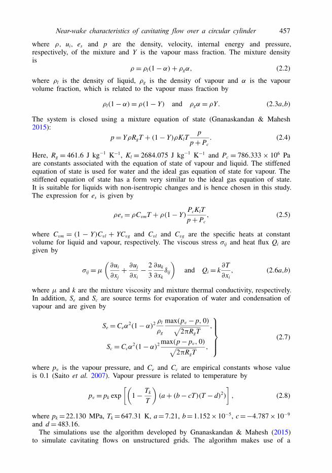
FIGURE 2. (Colour online) (a) Instantaneous isocontour (α = 0.1) of void fraction, and(b) time-averaged Cp distribution (——, LES; u, experiment of Rouse & McNown(1948)).

Gnanaskandan & Mahesh (2015) have evaluated this algorithm for a variety of flows,including a cavitating shock tube and turbulent cavitating flow over a hydrofoil and awedge.

3. Validation: cavitation over a hemispherical nose-shaped bodyWe consider partial cavitation over a hemispherical nose-shaped bluff body for

validation. We compare our LES results to the experimental results of Rouse &McNown (1948). The diameter of the hemisphere is D and the length of thecylindrical body is 50D. The extent of the domain is 50D in all directions. TheReynolds number based on the diameter of the hemisphere and free-stream velocityis ReD = 1.36 × 105 and the cavitation number is 0.4. The grid spacing used is0.002D in both streamwise and wall-normal directions and the grid is clusteredclose to the cavity inception region. A uniform grid spacing of 0.01D is used inthe circumferential direction. The solution is initialized with a void fraction ofα0 = 0.01. The non-dimensional time step tu∞/D = 2 × 10−5 and the solution isadvanced in a time-accurate manner. Figure 2(a) shows instantaneous isocontours ofvoid fraction which vary in the circumferential direction and are unsteady in time.Figure 2(b) compares the time-averaged Cp distribution to the experimental data(Rouse & McNown 1948); good agreement is obtained, indicating the suitability ofthe method in predicting bluff-body cavitation also.

4. Problem descriptionFigure 3 shows a schematic of the problem. A circular cylinder of diameter D

is placed at the centre of a circular domain of radius equal to 100D, chosen tominimize acoustic reflection from the far-field boundaries. The free-stream flow isspatially uniform and the velocity is in the positive x direction as shown in figure 3.The subscript ∞ is used to denote free-stream conditions and ρ∞, p∞, u∞ and µ∞denote free-stream density, pressure, velocity and dynamic viscosity, respectively.Free-stream conditions are imposed on all far-field boundaries. Acoustically absorbingboundary conditions (Colonius 2004) are applied in the sponge layer shown infigure 3. The term −γ (q − qref ) is added to the governing equations, where γ iszero outside the sponge layer, q denotes the vector of conservative variables and the


Flow

y

Sponge layer

Coarse mesh

50D

70D

100D

x

FIGURE 3. Computational domain illustrating sponge layer and region of coarse mesh(not to scale).

Reynolds number Cavitation number Initial void fraction(Re) (σ ) (α0)

200 2.0 0.01200 1.0 0.01200 0.7 0.01200 0.5 0.01200 1.0 0.005

3900 1.0 0.01

TABLE 1. Flow conditions used in the simulations.

subscript ‘ref ’ denotes the reference solution to which the flow inside the spongelayer is damped, which in this case is the free-stream value. Also the mesh is madecoarse in the far field to further reduce any reflections.

Table 1 lists the flow conditions for all the cases considered in this study. Here,cavitation number σ = (p∞ − pv)/(0.5ρ∞u2

∞) and the Reynolds number is givenby Re= (ρ∞u∞D)/µ∞. The simulations are initialized with a spatially uniform voidfraction (α0) that nucleates the cavitation. Insensitivity to computational grid anddomain size is demonstrated using two grids and two domain sizes for one case(Re = 200 and σ = 1.0). The mesh spacing for the fine grid is 0.005D × 0.01D inthe radial and azimuthal directions near the wall and stretches to 0.03D × 0.03Dat approximately 2D downstream and then further stretches to 0.07D × 0.07D ata distance of 5D downstream. The coarse grid has a near-wall mesh spacing of0.01D× 0.02D and stretches to 0.05D× 0.05D at approximately 2D downstream. Thecorresponding domain radii are 100D and 50D, respectively.

Figure 4 shows the lift and drag coefficients as functions of time for both the grids.Figure 5 shows the comparison of the mean and fluctuation of void fraction betweenthe two grids. Note that the solutions show good agreement, and the fine grid and thelarger domain have therefore been used for all the subsequent simulations at Re= 200.The mesh spacing and the spanwise extent for the 3D simulation are the same as that


130110 120100

0.5

0

–0.5

1.0

1.5

FIGURE 4. Comparison of lift and drag coefficient history showing grid convergencebetween two grids and domain insensitivity between two domains: – – – –, coarse grid,small domain; ——, fine grid, big domain.

2

4

0

2

4

0

2

4

0

2

4

00 0.2 0.4 0 0.2 0.4 0 0.05 0 0.1

(a) (b) (c) (d )

FIGURE 5. Comparison of (a,b) mean void fraction and (c,d) fluctuation in void fraction,for (a,c) x/D= 0.6 and (b,d) x/D= 2.0: ——, fine grid, big domain;@, coarse grid, smalldomain.

in the simulation of Verma & Mahesh (2012) for a single-phase flow at the sameReynolds number, where good agreement was obtained with experiment. The near-wallmesh spacing is 0.002D × 0.005D in size and stretches to 0.004D × 0.008D at adownstream location of 5D. A total of 80 points are used in the spanwise direction.Since the presence of vapour decreases the effective Reynolds number, this resolutionis deemed sufficient.

The nature of the instantaneous solution is illustrated in figure 6(a) using theRe = 200 and σ = 1.0 simulation. The void fraction contours show the presence


0 5 10 0

0 1.1 2.1 3.2 4.2 5.3 6.4

5 10

5

0

–5

5

0

–5

(a) (b)

Vapour in vortex core

Pressure wave

FIGURE 6. (Colour online) (a) Instantaneous snapshot showing coloured contours of voidfraction and contour lines showing pressure. (b) Instantaneous Mach-number contour.

of vapour immediately downstream of the cylinder as well as in the core of theKármán vortices downstream. The superposed contour lines of pressure show thepresence of ‘pressure waves’, which are compression waves that form when vapourpockets collapse in the higher-pressure regions downstream of the cylinder. Thespeed of sound drops significantly in regions of vapour, resulting in supersonic Machnumbers in some parts of the flow. Figure 6(b) reveals Mach numbers as high as6 in the cavitated shear layer immediately downstream of the cylinder. The largespatial variation in sound speed results in the pressure waves refracting through thenear-field vapour and impinging upon the cylinder. The Re = 3900 flow exhibitssimilar qualitative behaviour and is discussed in § 7.

The effect of σ on the time-averaged flow behind the cylinder as well as theunsteady loads on the cylinder are discussed below (§ 5) for Re= 200. The σ = 0.7and 0.5 flows exhibit a ‘low-frequency cavity detachment’ phenomenon, where apocket of vapour attached to the cylinder sheds downstream. This behaviour isanalysed in § 5.6. The σ value also affects the Kármán vortex shedding frequency,which is discussed in § 5.7. The influence of α0 is considered in § 6, and LES of theRe= 3900 flow is discussed in § 7.

5. Effect of cavitation number (σ )Cavitating flows at three different cavitation numbers (σ = 1.0, 0.7 and 0.5) are

considered and compared to the non-cavitating flow at σ = 2.0. The cavitation numberis varied by changing the free-stream velocity while keeping all other quantitiesconstant. The flow is seeded with a free-stream void fraction of α0 = 0.01.

5.1. Pressure on the cylinder surfaceFigure 7(a) shows the mean pressure coefficient on the cylinder surface. Here,θ = 0 and 180 correspond to the leading-edge stagnation point and trailing edge,respectively. In the absence of cavitation, the pressure coefficient decreases to its


0.5

0

–0.5

–1.0

1.0

0.5

0

1.0

1.5

2.0

2.5

3.0

30 60 90 120 150 1800 30 60 90 120 150 1800

(a) (b)

FIGURE 7. (Colour online) (a) Time-averaged Cp on the cylinder, and (b) time-averageddistribution of σlocal on the cylinder: ——, σ = 2.0; – – – –, σ = 1.0; – · – · –, σ = 0.7;— · · —, σ = 0.5.

minimum value at approximately 80 as the flow accelerates from the stagnationpoint, then increases as the flow decelerates, prior to becoming approximatelyconstant in the wake region at the trailing edge. Cavitation is seen to decreasethe magnitude of minimum Cp, with lower values of σ causing a larger decrease inmagnitude. This is because, once flow cavitates (close to the minimum Cp location),the pressure in the vapour region remains close to the vapour pressure; it does notfurther decrease with fluid acceleration. The upstream flow therefore sees lower valuesof favourable pressure gradient and the downstream flow experiences approximatelyconstant pressure.

Defining σlocal=2(p−pv)/ρ∞u2∞ and σ∞=2(p∞−pv)/ρ∞u2

∞ yields σlocal=Cp+σ∞.Figure 7(b) reveals small values for σlocal downstream of the minimum Cp location onthe cylinder surface for the cavitating flows. Also, for σ = 1.0 the mean pressure isalways above the vapour pressure, whereas for σ =0.7 and 0.5, the mean pressure fallsbelow the vapour pressure and recovers to values slightly above the vapour pressurenear the trailing edge of the cylinder. High-density fluid can therefore be present nearthe trailing edge, in the mean flow. This behaviour is illustrated in figure 8, whichshows contours of instantaneous and mean void fraction. Since, when σ = 1.0, onlythe instantaneous pressure falls below the vapour pressure, vapour is observed largelyin the core of the Kármán vortices. In contrast, when σ = 0.7 and 0.5, since the meanpressure in the near wake is also below the vapour pressure, vapour is also presentin substantial portions of the near wake. Figure 9 shows the variation of mean voidfraction and mixture density along the cylinder surface from the leading edge towardsthe trailing edge. Note the presence of higher-density fluid near the trailing edge, andthat the mean void fraction is not necessarily 1 due to vapour unsteadiness. Althoughvapour decreases the density of the mixture, the density is still skewed towards theliquid due to its significantly higher value.

5.2. Velocity divergence due to cavitationCavitation causes density change, which implies a considerable change in thedivergence of the velocity field. Figure 10 shows the mean velocity divergence(∇ · V) contours for all the cavitating cases. Expansion caused due to cavitation


–1

0

1

–1

0

1

–1

0

1

–1

0

1

–1

0

1

–1

0

1

0 2 4 6 8 0 2 4 6 8

0 2 4 6 8 0 2 4 6 8

0 2 4 6 8 0 2 4 6 8

(a) (b)

(c) (d )

(e) ( f )

0.05 0.22 0.39 0.56 0.72 0.05 0.15 0.25 0.35 0.45

FIGURE 8. (Colour online) Instantaneous (a,c,e) and mean (b,d,f ) void fraction contoursfor (a,b) σ = 1.0, (c,d) σ = 0.7 and (e,f ) σ = 0.5.

30 60 90 120 150 1800

1.0

0.2

0.4

0.6

0.8

1.0

0.2

0.4

0.6

0.8

0

FIGURE 9. (Colour online) Variation of density (solid) and void fraction (dashed) alongthe cylinder surface as a function of azimuthal location: σ = 2.0 (black), σ = 1.0 (red),σ = 0.7 (green), σ = 0.5 (blue).

can be seen as positive divergence and, as the flow cavitates more, the region ofpositive ∇ · V also increases due to the increased amount of vapour. It is interestingto note a compression region (negative ∇ · V) downstream of the expansion region,and the magnitude of this compression region appears to decrease as the cavitationnumber reduces. This behaviour can be understood by revisiting the mean voidfraction contours in figure 8. For σ = 1.0, there is a large decrease in void fractioncorresponding to the region of negative divergence. This is a result of the cavitating


0 0.5 1.0 1.5 2.0–0.5 0 0.5 1.0 1.5 2.0–0.5

0 0.5 1.0 1.5 2.0–0.5

0.5

0

–0.5

–1.0

1.0

0.5

0

–0.5

–1.0

1.0

0.5

0

–0.5

–1.0

–1.0 –0.6 –0.2 0.2 0.6

–1.0 –0.6 –0.2 0.2 0.6 –1.0 –0.6 –0.2 0.2 0.6

1.0

(a) (b)

(c)

FIGURE 10. (Colour online) Contours of divergence of velocity field for (a) σ = 1.0,(b) σ = 0.7 and (c) σ = 0.5.

vortex being shed from the body, which takes away vapour from close to the body,leading to a sharp decrease in void fraction in the mean. However, we observe that,for σ = 0.7 and 0.5, the void fraction does not decrease as much as in σ = 1.0, sincefor these cases the cavitating vortex sheds from the attached cavity at a downstreamlocation. Thus this compression region is an indication of some amount of vapourbeing converted back to water.

5.3. Boundary layer on the cylinder surfaceThe pressure along the cylinder surface affects the evolution of the boundary layer.Figure 11 shows boundary layer velocity profiles at four different azimuthal locationsfor σ = 2.0 and 0.5. Mean values are shown on top and root mean square valueson the bottom. The azimuthal locations θ = 70, 90, 110 and 130 are chosento represent regions of favourable pressure gradient, minimum pressure, adversepressure gradient and separated flow, respectively. Figure 11 contrasts only σ = 2.0(non-cavitating) and 0.5 (cavitating) cases for clarity. Here, uθ is the tangentialvelocity and r is the normal distance from the cylinder at any given azimuthallocation. Cavitation causes expansion (positive dilatation) at the inception location,which causes the flow upstream to decelerate as seen in figure 11. For instance,the maximum velocity in the boundary layer (uθmax/u∞) drops to a value of 1.10for σ = 0.5 from a value of 1.34 for σ = 2.0 at an azimuthal location of 70. The


0

1

2

3

4

0

1

2

3

4

5

0

1

2

3

4

0

1

2

3

4

0

1

2

3

4

1

2

3

4

5

0

1

2

3

4

5

1

2

3

4

0.5 1.0 0.5 1.0 0 0.5 1.0 0 0.5 1.0

0 0.05 0 0.05 0.10 0 0.05 0.10 0 0.1 0.2

(a) (b) (c) (d)

(e) ( f ) (g) (h)

FIGURE 11. Mean (a–d) and root mean square (e–h) boundary layer profiles at fourazimuthal locations θ = 70 (a,e), 90 (b,f ), 110 (c,g) and 130 (d,h): ——, σ = 2.0;and – – – –, σ = 0.5.

fluctuation levels of the cavitating flow are much lower at the first two locations,indicating that the flow becomes steady due to cavitation. The location wheremaximum velocity in the boundary layer occurs is also shifted away from the wallfor the cavitating flow as a result. The magnitude of the maximum velocity in theboundary layer (uθmax ) and the location of its occurrence are plotted as a function of θin figure 12 for all four cases. Note that the boundary layer thickens with decreasingcavitation number. Also the magnitude of uθmax initially increases in the favourablepressure gradient region and then drops after 80. The drop in magnitude of uθmax

is rapid for σ = 2.0 after 90 when compared to the cavitating flow, which pointsto a rapid thickening of the boundary layer leading to separation. The location ofmaximum velocity is shifted away from the wall as the flow cavitates more, and thisdifference between cavitating and non-cavitating flow increases further as we movecloser to the trailing edge.


60 80 100 120 140 60 80 100 120 140

1.0

1.1

1.2

1.3

1.4

1.0

1.2

1.4

1.6

1.8

0.6

0.8

(a) (b)

FIGURE 12. (Colour online) (a) Variation of maximum velocity in the boundary layer asa function of azimuthal location, and (b) variation of location of maximum velocity inthe boundary layer as a function of azimuthal location: ——, σ = 2.0; – – – –, σ = 1.0;– · – · –, σ = 0.7; — · · —, σ = 0.5.

0.1

0

0.2

0.3

30 60 90 120 150 1800

FIGURE 13. (Colour online) Time-averaged skin friction coefficient distribution on thecylinder: ——, σ = 2.0: – – – –, σ = 1.0; – · – · –, σ = 0.7; — · · —, σ = 0.5.

Figure 13 shows the time-averaged skin friction distribution along the cylinder. Themagnitude of Cf initially increases in the favourable pressure gradient region and thendrops as the boundary layer thickens due to adverse pressure gradient. Note that thecavitating flows have a reduced skin friction value compared to σ = 2.0 up to 80due to the deceleration caused by the vapour cavity. Flow expansion due to cavitationalso causes the flow downstream of the inception location to accelerate. This canbe seen in the form of a local increase in skin friction coefficient in figure 13 forσ = 1.0, 0.7 and 0.5 at approximately 80. The flow separates under the influence ofadverse pressure gradient at approximately 110 for σ = 2.0. The separation locationfor the cavitated flows, however, shifts downstream to approximately 120 for σ = 1.0and 0.7 and to approximately 125 for σ = 0.5. This behaviour is in contrast to theobservations of Arakeri (1975) and Ramamurthy & Bhaskaran (1977), who found thatthe separation point moves upstream as the flow cavitates more. The main reason for


0

0.2

0.4

0.6

0

0.05

0.10

0.15

0.5

1.0

1.5

2.0

5 10 15

0.5

1.0

1.5

2.0

0.5 2.5 4.5 6.5 8.5 0.5 2.5 4.5 6.5 8.5

(a) (b)

(c)

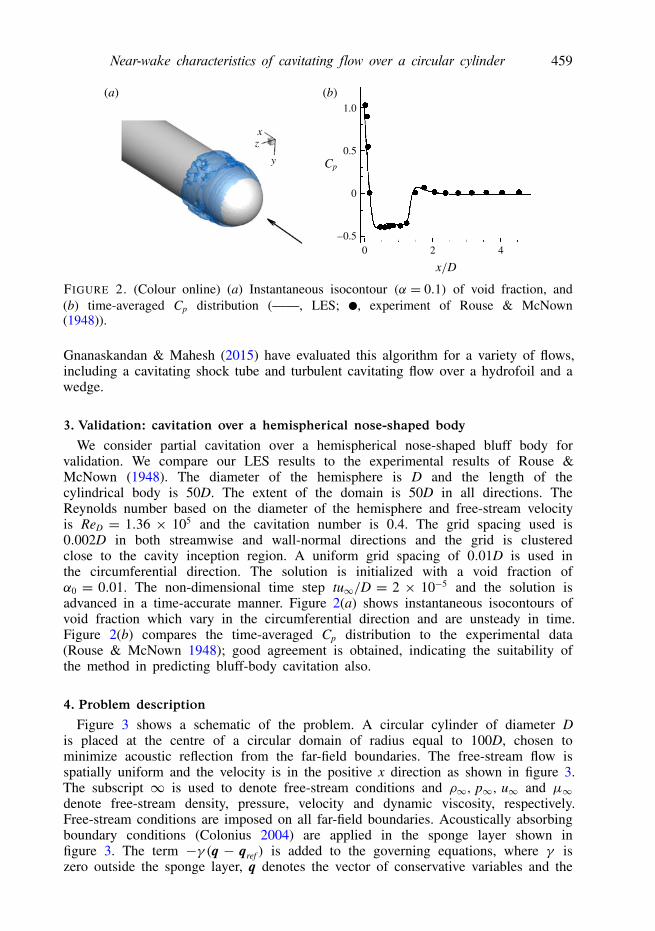
FIGURE 14. (Colour online) Variation of (a) α and (b) α′2 with downstream distance inthe wake: ——, σ = 1.0; – – – –, σ = 0.7; – · – · –, σ = 0.5. (c) Variation of normalizedcavity length with cavitation number: ——, experimental fit (Rao & Chandrasekhara1976);@, Re= 200;E, Re= 3900.

this discrepancy is the fact that the homogeneous mixture model predicts that theinception point is upstream of the separation point. The cavitation criterion in themodel is simply based on the difference between the local pressure and the vapourpressure, and hence cavitation occurs as soon as the pressure drops below the vapourpressure (although there is a finite rate at which vapour is produced). However, inreality, cavitation does not occur immediately at the location where the pressure dropsbelow the vapour pressure, but occurs downstream of the separation point. In thenumerical simulations, with the separation point downstream of the inception point,the acceleration induced by expansion pushes the separation point further downstreamas the flow cavitates more. In contrast, in the experiments of Arakeri (1975) andRamamurthy & Bhaskaran (1977), the separation point is ahead of the inception pointand the cavitation-induced expansion causes flow deceleration upstream leading to anearlier separation.

5.4. Cavity lengthThe mean cavity length increases progressively as the cavitation number decreases.The mean length of the cavity is computed from figure 14(a) as the location


10010–1 102101 10010–110–2 102101 10010–110–2 102101

120 140 160 180 150 200 250 300 150 200 250 300 350 400

10–6

10–12

10010–5

10–15

10–10

10–20

10–4

10–14

10–9

10–19

0.5

0

–0.5

1.0

0.5

0

–0.5

1.0

0.5

0

1.0

PSD

(a) (b) (c)

(d ) (e) ( f )

FIGURE 15. (Colour online) Lift and drag history (a–c) and their spectra (d–f ) for(a,d) σ = 1.0, (b,e) σ = 0.7 and (c,f ) σ = 0.5: ——, CL; – – – –, CD.

downstream where α reaches a value of 0.05 after its initial increase. This figurealso shows the maximum α obtained in the near wake. As the cavitation numberdecreases, it is expected that more vapour will be formed in the wake. Interestingly,the αmax is higher for σ = 1.0, when compared to σ = 0.7. This is due to the effect ofthe low-frequency cavity detachment when σ = 0.7, which will be discussed in detailin § 5.6. The root mean square values of void fraction are plotted in figure 14(b)and show a trend similar to the mean value. The mean cavity length as a functionof cavitation number is shown in figure 14(c) and shows that the length increases asthe cavitation number is reduced. The plot also shows the mean cavity length as afunction of a modified cavitation number σm = (p− pv)/(0.5ρu2

max). Here, umax is themaximum mean velocity in the boundary layer, which is obtained from figure 12(a).This modification was first suggested by Rao & Chandrasekhara (1976), who observedthat, when the mean cavity length was plotted against σ , a family of curves wereobtained for different Reynolds numbers for cavitating flow over a circular cylinder.Hence they introduced the modified cavitation number, which unified the differentfamilies of curves onto a single curve. We observe in figure 14(c) that the mean cavitylength obtained at a lower Reynolds number also collapses onto this experimental fitif the modified cavitation number is used. Given that the experimental fit is obtainedpurely based on experiments at high Reynolds number (typically 105), it is interestingto see that the data from our low-Reynolds-number simulations also collapse ontothis curve.

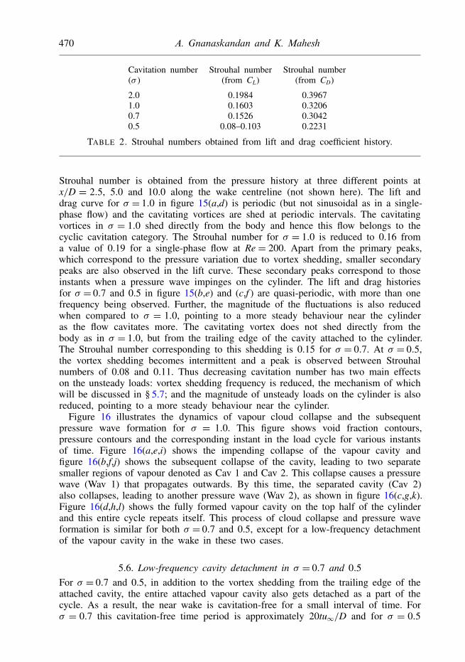
5.5. Unsteady loads on the cylinderFigure 15 shows the unsteady characteristics of the flow in the form of lift and draghistory and their corresponding spectra in the frequency domain. The Strouhal number( fD/u∞, where f is the vortex shedding frequency) computed from the lift and draghistories is tabulated in table 2. Further, it is also verified that the same shedding


Cavitation number Strouhal number Strouhal number(σ ) (from CL) (from CD)

2.0 0.1984 0.39671.0 0.1603 0.32060.7 0.1526 0.30420.5 0.08–0.103 0.2231

TABLE 2. Strouhal numbers obtained from lift and drag coefficient history.

Strouhal number is obtained from the pressure history at three different points atx/D = 2.5, 5.0 and 10.0 along the wake centreline (not shown here). The lift anddrag curve for σ = 1.0 in figure 15(a,d) is periodic (but not sinusoidal as in a single-phase flow) and the cavitating vortices are shed at periodic intervals. The cavitatingvortices in σ = 1.0 shed directly from the body and hence this flow belongs to thecyclic cavitation category. The Strouhal number for σ = 1.0 is reduced to 0.16 froma value of 0.19 for a single-phase flow at Re = 200. Apart from the primary peaks,which correspond to the pressure variation due to vortex shedding, smaller secondarypeaks are also observed in the lift curve. These secondary peaks correspond to thoseinstants when a pressure wave impinges on the cylinder. The lift and drag historiesfor σ = 0.7 and 0.5 in figure 15(b,e) and (c,f ) are quasi-periodic, with more than onefrequency being observed. Further, the magnitude of the fluctuations is also reducedwhen compared to σ = 1.0, pointing to a more steady behaviour near the cylinderas the flow cavitates more. The cavitating vortex does not shed directly from thebody as in σ = 1.0, but from the trailing edge of the cavity attached to the cylinder.The Strouhal number corresponding to this shedding is 0.15 for σ = 0.7. At σ = 0.5,the vortex shedding becomes intermittent and a peak is observed between Strouhalnumbers of 0.08 and 0.11. Thus decreasing cavitation number has two main effectson the unsteady loads: vortex shedding frequency is reduced, the mechanism of whichwill be discussed in § 5.7; and the magnitude of unsteady loads on the cylinder is alsoreduced, pointing to a more steady behaviour near the cylinder.

Figure 16 illustrates the dynamics of vapour cloud collapse and the subsequentpressure wave formation for σ = 1.0. This figure shows void fraction contours,pressure contours and the corresponding instant in the load cycle for various instantsof time. Figure 16(a,e,i) shows the impending collapse of the vapour cavity andfigure 16(b,f,j) shows the subsequent collapse of the cavity, leading to two separatesmaller regions of vapour denoted as Cav 1 and Cav 2. This collapse causes a pressurewave (Wav 1) that propagates outwards. By this time, the separated cavity (Cav 2)also collapses, leading to another pressure wave (Wav 2), as shown in figure 16(c,g,k).Figure 16(d,h,l) shows the fully formed vapour cavity on the top half of the cylinderand this entire cycle repeats itself. This process of cloud collapse and pressure waveformation is similar for both σ = 0.7 and 0.5, except for a low-frequency detachmentof the vapour cavity in the wake in these two cases.

5.6. Low-frequency cavity detachment in σ = 0.7 and 0.5For σ = 0.7 and 0.5, in addition to the vortex shedding from the trailing edge of theattached cavity, the entire attached vapour cavity also gets detached as a part of thecycle. As a result, the near wake is cavitation-free for a small interval of time. Forσ = 0.7 this cavitation-free time period is approximately 20tu∞/D and for σ = 0.5


132 134 136 132 134 136 132 134 136 132 134 136

0 5 10 0 5 10 0 5 10 0 5 10

0 2 4 6 0 2 4 6 0 2 4 6 0 2 4 6

–3

0

3

–5

0

5

0

0.6

1.2

Wav 1 Wav 2Wav 1

(a) (b) (c) (d )

(e) ( f ) (g)

(k)

(h)

(l)(i) ( j)

Cav 2Cav 1

FIGURE 16. (Colour online) Vapour collapse dynamics for σ = 1.0.

120 140 160 180 200 150 200 250 300 350 400

0.5

0

1.0

0.5

0

–0.5

1.0

(a) (b)

FIGURE 17. (Colour online) Time history of lift showing two phenomena in a single cyclefor (a) σ = 0.7 and (b) σ = 0.5: ——, CL; – – – –, CD.

it is approximately 30tu∞/D. The frequency corresponding to this detachment can beobserved as a peak in the drag spectra in figure 15(b,c) and is computed to be 0.0218for σ = 0.7 and 0.0102 for σ = 0.5. The lift curves in figure 17(a,b) suggest thatthere are two distinct parts within one cycle: one with a relatively low variation inCL and another with a higher variation in CL. The first part with low CL variationcorresponds to the time when the vapour cavity is attached to the body. Since thepressure in the vapour region is close to the vapour pressure, the variation in CL is


very small. As the vapour cavity detaches, water in the wake causes higher variationsin the lift coefficient.

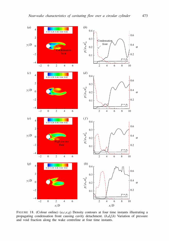
The mechanism behind this detachment is illustrated in figure 18, where a series ofsnapshots show the presence of a propagating condensation front that causes cavitydetachment from the base of the cylinder. Figure 18(a,c) shows the propagation ofthe condensation front towards the low-pressure base. This causes the pressure inthe base to increase, which can be seen as a small patch of high-density fluid nearthe base of the cylinder (figure 18e). This causes the vapour cavity to detach, asseen in figure 18(g). The detached cavities advect downstream, leaving the near-wakecavitation free for a while. The presence of a condensation front can also be seenfrom the line plots in the figure. The pressure increase and the corresponding voidfraction decrease close to x/d = 2.0 seen in figure 18(b,d) is the condensation front.Figure 18( f,h) also shows the presence of high-density (low-void-fraction) fluid nearthe base once the cavity detaches.

The low-frequency cavity detachment in σ = 0.7 means that the entire near wakeis cavitation-free for a while. This effectively reduces the time-averaged void fractionin those regions where cavitation is absent during some part of the cycle. Hence themaximum time-averaged void fraction of σ = 0.7 is lower than that of σ = 1.0, asseen in figure 14(a). This cavitation-free period is a substantial part of one cycle forσ = 0.7 (20tu∞/D out of 45tu∞/D) when compared to the σ = 0.5 (30tu∞/D out of100tu∞/D) where the cavitation-free period is for a lesser amount of time in the cycle.Thus this effect is not pronounced in σ = 0.5 when compared to σ = 0.7.

5.7. Mechanism of vortex shedding frequency reductionAt low Reynolds number, the vorticity transported into the wake from the boundarylayers on the cylinder is diffused away from the shear layer predominantly byviscous action. As the Reynolds number increases, viscous diffusion alone cannotkeep up with the increased vorticity production from the boundary layers, and sovortices break away at regular intervals, constituting vortex shedding (Strykowski &Sreenivasan 1990). Gerrard (1966) observed vortex street formation to be a functionof two length scales: the formation length and diffusion length. The formation lengthlf is defined as the distance downstream of the cylinder along the centreline wherethe streamwise velocity fluctuations are maximum, and the diffusion length ld isthe width to which the free shear layers diffuse. He found that the vortex sheddingfrequency could be reduced if the shear layer vorticity was reduced over a criticaldiffusion length, which in turn increases the formation length.

In order to understand the mechanism of vortex shedding suppression due tocavitation, we first compute the formation length (lf ) by plotting the streamwisevelocity fluctuations in figure 19 for σ = 2.0, 1.0, 0.7 and 0.5. The formation lengthis seen to increase with decreasing cavitation number, which signifies a reduction inshedding frequency (Gerrard 1966). It is also worthwhile to note that the magnitudeof the streamwise velocity fluctuation also increases as the flow cavitates. This pointsto higher oscillations at the cavity closure as σ is lowered. Also shown in figure 19are the instantaneous vorticity contours, showing fewer vortices being shed over agiven distance as the cavitation number is reduced.

Figure 20 shows the mean vorticity distribution in the top half of the shearlayer. The arguments presented here can be applied to the bottom half also bysymmetry. Note that the magnitude of negative vorticity in the top shear layerdecreases progressively as the cavitation number decreases. Thus cavitating flow has


–2 0 2 4 6

–2 0 2 4 6

–2 0 2 4 6

–2 0 2 4 6 2 4 6 8 10

2 4 6 8 10

2 4 6 8 10

2 4 6 8 10

2

4

0

–2

–4

2

4

0

0.10 0.28 0.46 0.64 0.82

0.10 0.28 0.46 0.64 0.82

0.10 0.28 0.46 0.64 0.82

0.10 0.28 0.46 0.64 0.82

–2

–4

2

4

0

–2

–4

2

4

0

–2

–4

0.1

0.2

0.3

0.4

0.1

0.2

0.3

0.4

0.1

0.2

0.3

0.4

0.1

0.2

0.3

0.4

0.2

0.4

0.6

0.2

0.4

0.6

0.2

0.4

0.6

0.2

0.4

0.6

(a) (b)

(c) (d)

(e) ( f )

(g) (h)

High densityfluid

Condensationfront

Condensationfront

FIGURE 18. (Colour online) (a,c,e,g) Density contours at four time instants illustrating apropagating condensation front causing cavity detachment. (b,d,f,h) Variation of pressureand void fraction along the wake centreline at four time instants.


2 4 6 8 10

2 4 6 8 10

2 4 6 8 10

2 4 6 8 10

0.08

0.06

0.04

0.02

0

0.08

0.06

0.04

0.02

0

0.08

0.06

0.04

0.02

0

0.08

0.06

0.04

0.02

0

0 5 10 15 20 25 30

0 5 10 15 20 25 30

0 5 10 15 20 25 30

0

0.05 0.25 0.45 0.65 0.85

5 10 15 20 25 30

5

0

–5

5

0

–5

5

0

–5

5

0

–5

(a) (b)

(c) (d )

(e) ( f )

(g) (h)

FIGURE 19. (Colour online) (a,c,e,g) Formation length and (b,d,f,h) instantaneous vorticitycontour coloured with density for: (a,b) σ = 2.0, lf /D= 1.45; (c,d) σ = 1.0, lf /D= 2.35;(e,f ) σ = 0.7, lf /D= 4.19; and (g,h) σ = 0.5, lf /D= 7.01.

lesser vorticity across a given shear layer width and the reason for this reduction isexplained below using the vorticity equation,

∂ω

∂t=−(v · ∇)ω+ (ω · ∇)v −ω(∇ · v)+ 1

ρ2(∇ρ ×∇p)+∇× ∇ · τ

ρ. (5.1)


1.0

0

0.2

0.4

0.6

0.8

0

0

0

1.0

0.2

0.4

0.6

0.8

1.0

0.2

0.4

0.6

0.8

1.0

0.2

0.4

0.6

0.8

0

0

0

1.0

0.2

0.4

0.6

0.8

1.0

0.2

0.4

0.6

0.8

1.0

0.2

0.4

0.6

0.8

0

0

0

1.0

0.2

0.4

0.6

0.8

1.0

0.2

0.4

0.6

0.8

1.0

0.2

0.4

0.6

0.8

0 0.5 0 0.5 0 0.5

0 0.5 0 0.5 0 0.5

0 0.5 0 0.5 0 0.5

0 0.5

(a)

(b) (c) (d )

(e) ( f ) (g)

(h) (i) ( j)

1.1–3.0–5.0 –0.9 3.2

1.1–3.0–5.0 –0.9 3.2

1.1–3.0–5.0 –0.9 3.2

1.1–3.0–5.0 –0.9 3.2

0.4–1.2–2.0 –0.4 1.3 1.1–1.2–2.0 –0.5 –0.3 1.8

1.1–1.2–2.0 –0.5 –0.3 1.80.4–1.2–2.0 –0.4 1.3

0.4–1.2–2.0 –0.4 1.3 0.4–1.2–2.0 –0.4 1.3

FIGURE 20. (Colour online) Mean vorticity contour (a,b,e,h), mean baroclinic vorticity(c,f,i) and mean vorticity dilatation (d,g,j) for (a) σ = 2.0, (b–d) σ = 1.0, (e–g) σ = 0.7and (h–j) σ = 0.5.

For a constant-density non-cavitating flow, the vorticity dilatation term (ω(∇ · v)) andthe baroclinic vorticity ((1/ρ2)(∇ρ ×∇p)) terms are zero. However, for a cavitatingflow, these values are non-zero. Figure 20 shows the contribution of the meanbaroclinic vorticity term. At the inception location, baroclinic vorticity is produced


Cavitation number Circulation Formation length(σ ) (Γ ) (lf /D)

2.0 4.80 1.451.0 4.03 2.350.7 3.08 4.190.5 2.78 7.01

TABLE 3. Values of circulation Γ and formation length lf .

because pressure becomes a function of both vapour mass fraction and density,thus causing a misalignment between pressure and density gradients. The baroclinicterm produces more negative vorticity on the top half for all the cavitating cases thusincreasing the total vorticity in the shear layer. The main reason for vorticity reductionis the vorticity dilatation term. As seen in figure 10, there is a large region of positivedivergence (expansion) corresponding to the vapour region. The magnitude of vorticitydilatation is also shown in figure 20. Note that this term appears in the right-handside of the vorticity equation with a negative sign. The blue region corresponds tovorticity dilatation, which reduces the vorticity in the shear layer. The compressionregion (discussed in § 5.2) causes the vorticity to increase downstream, shown as thered contours: however, the larger influence of the expansion region results in a netdecrease in vorticity.

To quantify the extent of vorticity reduction, the circulation in the shear layeris computed as

∮V · dl over a rectangular domain from 0.5 < x/D < 4.0 and

0 < y/D < 1.0, where the centre of the cylinder lies at the origin. As the flowcavitates more, the amount of circulation decreases, pointing to reduced vorticity inthe shear layer. Table 3 lists the values of circulation and the corresponding formationlengths for all the cases. Thus the presence of vapour in the wake causes dilatationof vorticity, resulting in a reduction of the vortex shedding frequency.

6. Effect of initial void fractionIn this section, we discuss the effect of initial void fraction (α0) on the flow field

by simulating σ = 1.0 flow with α0= 0.005 and comparing it to α0= 0.01. The initialvoid fraction values of 1 % and 0.5 % are large compared to those used in controlledexperiments. However, these values are chosen to reduce the acoustic stiffness of thesystem. The main effect of changing α0 is the change in free-stream speed of sound.At a temperature of 293 K and a pressure of 1 bar, the speed of sound in a mixturewith α0 = 0.01 is 100.24 m s−1, while that at α0 = 0.005 is 141.07 m s−1. Hencepressure waves propagating in the medium will travel at these substantially differentspeeds, which would affect related phenomena. However, phenomena that are drivenlargely by inertia (e.g. cavitation in shear layer, vortex shedding) are not expected tovary significantly.

6.1. Mean Cp and Cf distributions on the cylinderThe time-averaged Cp distribution and Cf distribution are shown as a function of θin figure 21(a,b) for both α0 = 0.01 and 0.005. Note that neither Cp nor Cf varysignificantly for different α0. The time-averaged load on a cylinder is predominantlydue to the alternate vortex shedding, which is not affected significantly by change in


30 60 90 120 150 1800 30 60 90 120 150 1800

0.5

0

–0.5

–1.0

1.0

0.1

0

0.2

0.3(a) (b)

FIGURE 21. (a) Time-averaged Cp distribution on the cylinder, and (b) time-averaged Cfdistribution on the cylinder: ——, α0 = 0.01;E, α0 = 0.005.

–3

–2

–1

0

1

2

3

–3

–2

–1

0

1

2

3

–2 0 2 4 –2 0 2 4

0.10 0.20 0.30 0.39 0.49 0.10 0.20 0.30 0.39 0.49

(a) (b)

FIGURE 22. (Colour online) Mean void fraction contour for (a) α0 = 0.01 and(b) α0 = 0.005.

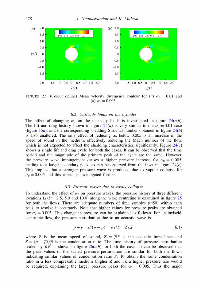
acoustic speed. The inflection point (at θ = 80) in the Cf curve that indicates thecavity inception location (as discussed in § 5) also remains unchanged between thetwo flows. Figure 22 shows the mean void fraction contours for both the flows. Thecavity shape and cavity length (lcav/D= 2.71) remain largely unaffected. According tothe continuity equation, ∂uj/∂xj=−(1/ρ)(Dρ/Dt), the divergence of velocity dependson the material derivative of density. The main contribution to density change comesfrom the phase change, which has a time scale of its own due to the finite rate. Sincephase change does not occur on the acoustic scale, changing the speed of sound doesnot significantly affect the divergence of velocity and hence its interplay with theboundary layer is also largely unaffected. Figure 23 shows contours of mean velocitydivergence for both α0 = 0.01 and 0.005. The contours are identical, confirming thefact that velocity divergence is not affected by the initial void fraction.


0.5

1.0

1.5

2.0

0

–0.5

–1.0

–1.5

0–1.0–2.0 –0.5–1.5 0.5 1.0 1.5 2.0

0.5

1.0

1.5

2.0

0

–0.5

–1.0

–1.5

0–1.0–2.0 –0.5–1.5 0.5 1.0 1.5 2.0

(a) (b)

–0.37–2.00 0.45–1.18 1.27 –0.37–2.00 0.45–1.18 1.27

FIGURE 23. (Colour online) Mean velocity divergence contour for (a) α0 = 0.01 and(b) α0 = 0.005.

6.2. Unsteady loads on the cylinderThe effect of changing α0 on the unsteady loads is investigated in figure 24(a,b).The lift and drag history shown in figure 24(a) is very similar to the α0 = 0.01 case(figure 15a), and the corresponding shedding Strouhal number obtained in figure 24(b)is also unaltered. The only effect of reducing α0 below 0.005 is an increase in thespeed of sound in the medium, effectively reducing the Mach number of the flow,which is not expected to affect the shedding characteristics significantly. Figure 24(c)shows a single lift and drag cycle for both the cases. It can be observed that the timeperiod and the magnitude of the primary peak of the cycle are the same. However,the pressure wave impingement causes a higher pressure increase for α0 = 0.005,leading to a larger secondary peak, as can be observed from the inset in figure 24(c).This implies that a stronger pressure wave is produced due to vapour collapse forα0 = 0.005 and this aspect is investigated further.

6.3. Pressure waves due to cavity collapseTo understand the effect of α0 on pressure waves, the pressure history at three differentlocations (x/D= 2.5, 5.0 and 10.0) along the wake centreline is examined in figure 25for both the flows. There are adequate numbers of time samples (≈50) within eachpeak to resolve it accurately. Note that higher values for pressure peaks are obtainedfor α0 = 0.005. This change in pressure can be explained as follows. For an inviscid,isentropic flow, the pressure perturbation due to an acoustic wave is

p− p= c2(ρ − ρ)= ρ c2S= Z cS, (6.1)

where c is the mean speed of sound, Z ≡ ρ c is the acoustic impedance andS ≡ (ρ − ρ)/ρ is the condensation ratio. The time history of pressure perturbationscaled by ρ c2 is shown in figure 26(a,b) for both the cases. It can be observed thatthe peak values of the scaled pressure perturbation are similar for both the flows,indicating similar values of condensation ratio S. To obtain the same condensationratio in a less compressible medium (higher Z and c), a higher pressure rise wouldbe required, explaining the larger pressure peaks for α0 = 0.005. Thus the major


12010090 130110 100 10110–1 102

100

10–6

10–12

0.5

1.0

0

–0.5

PSD

St

(a) (b)

(c)

116

116

120118

115

110 112 114

0.2

0.4

0.3

0.5

0.5

1.0

0

–0.5

FIGURE 24. (Colour online) (a) Lift and drag history for α0 = 0.005. (b) Power spectraldensity for α0 = 0.005: ——, CL; – – – –, CD. (c) Comparison of a single lift and dragcycle:E, α0 = 0.01; and ——, α0 = 0.005.

1.0

0

0.2

0.4

0.6

0.8

1.0

0

0.2

0.4

0.6

0.8

150 152 154 156 158 160 112 114 116 118 120

(a) (b)

FIGURE 25. Pressure history at three different locations along the wake centreline for(a) α0 = 0.01 and (b) α0 = 0.005: ——, x/D= 2.5; – – – –, x/D= 5.0;E, x/D= 10.0.


–0.1

0

0.1

0.2

0.3

–0.1

0

0.1

0.2

0.3

150 152 154 156 158 160 112 114 116 118 120

(a) (b)

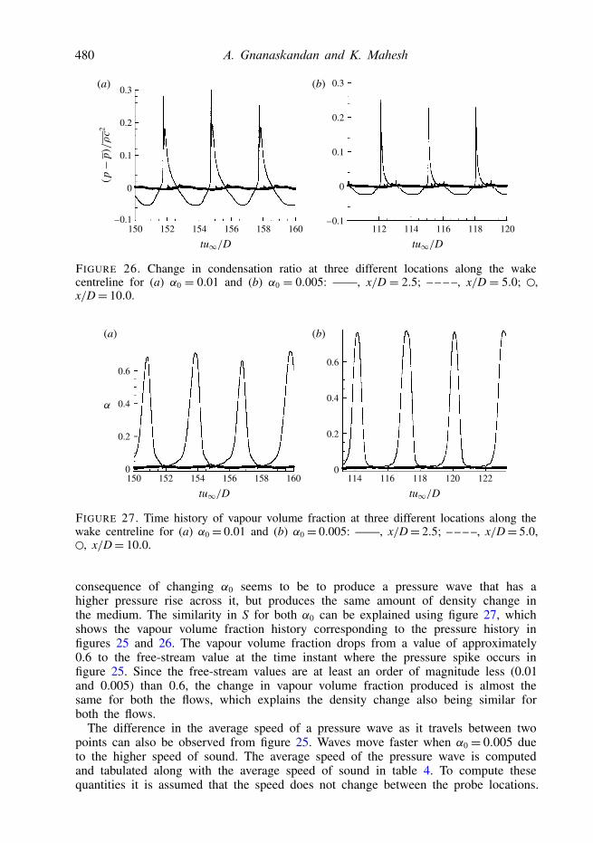
FIGURE 26. Change in condensation ratio at three different locations along the wakecentreline for (a) α0 = 0.01 and (b) α0 = 0.005: ——, x/D = 2.5; – – – –, x/D = 5.0; E,x/D= 10.0.

150 152 154 156 158 160 114 116 118 120 122 0

0.2

0.4

0.6

0

0.2

0.4

0.6

(a) (b)

FIGURE 27. Time history of vapour volume fraction at three different locations along thewake centreline for (a) α0 = 0.01 and (b) α0 = 0.005: ——, x/D= 2.5; – – – –, x/D= 5.0,E, x/D= 10.0.

consequence of changing α0 seems to be to produce a pressure wave that has ahigher pressure rise across it, but produces the same amount of density change inthe medium. The similarity in S for both α0 can be explained using figure 27, whichshows the vapour volume fraction history corresponding to the pressure history infigures 25 and 26. The vapour volume fraction drops from a value of approximately0.6 to the free-stream value at the time instant where the pressure spike occurs infigure 25. Since the free-stream values are at least an order of magnitude less (0.01and 0.005) than 0.6, the change in vapour volume fraction produced is almost thesame for both the flows, which explains the density change also being similar forboth the flows.

The difference in the average speed of a pressure wave as it travels between twopoints can also be observed from figure 25. Waves move faster when α0= 0.005 dueto the higher speed of sound. The average speed of the pressure wave is computedand tabulated along with the average speed of sound in table 4. To compute thesequantities it is assumed that the speed does not change between the probe locations.


Location Initial void fraction Avg. condensation wave speed Avg. sound speed

(x/D) (α0) (uc/u∞) (c/u∞)

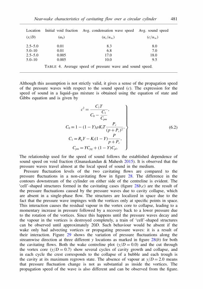
2.5–5.0 0.01 8.3 8.05.0–10 0.01 6.8 7.02.5–5.0 0.005 17.0 18.05.0–10 0.005 10.0 9.5

TABLE 4. Average speed of pressure wave and sound speed.

Although this assumption is not strictly valid, it gives a sense of the propagation speedof the pressure waves with respect to the sound speed (c). The expression for thespeed of sound in a liquid–gas mixture is obtained using the equation of state andGibbs equation and is given by

c2 = C1T

C0 − C1

Cpm

,

C0 = 1− (1− Y)ρKlTPc

(p+ Pc)2,

C1 = RgY −Kl(1− Y)P

p+ Pc,

Cpm = YCpg + (1− Y)Cpl.

(6.2)

The relationship used for the speed of sound follows the established dependence ofsound speed on void fraction (Gnanaskandan & Mahesh 2015). It is observed that thepressure waves travel almost at the local speed of sound in the medium.

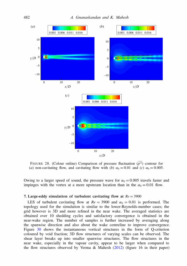
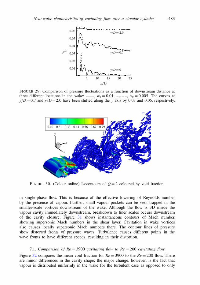
Pressure fluctuation levels of the two cavitating flows are compared to thepressure fluctuations in a non-cavitating flow in figure 28. The difference in thecontours downstream of the cylinder on either side of the centreline is evident. The‘cell’-shaped structures formed in the cavitating cases (figure 28b,c) are the result ofthe pressure fluctuations caused by the pressure waves due to cavity collapse, whichare absent in a single-phase flow. The structures are localized in space due to thefact that the pressure wave impinges with the vortices only at specific points in space.This interaction causes the residual vapour in the vortex core to collapse, leading to amomentary increase in pressure followed by a recovery back to a lower pressure dueto the rotation of the vortices. Since this happens until the pressure waves decay andthe vapour in the vortices is destroyed completely, a train of ‘cell’-shaped structurescan be observed until approximately 20D. Such behaviour would be absent if thewake only had advecting vortices or propagating pressure waves: it is a result oftheir interaction. Figure 29 shows the variation of pressure fluctuations along thestreamwise direction at three different y locations as marked in figure 28(b) for boththe cavitating flows. Both the wake centreline plot (y/D = 0.0) and the cut throughthe vortex core (y/D = 0.7) show several cycles of cavity growth and collapse, andin each cycle the crest corresponds to the collapse of a bubble and each trough isthe cavity at its maximum regrown state. The absence of vapour at y/D= 2.0 meansthat pressure fluctuation change is not as substantial as inside the vortices. Thepropagation speed of the wave is also different and can be observed from the figure.


5

0

10

–5

–10

5

0

10

–5

–10

5

0

10

–5

–10

10 200 10 200

10 200

0.001 0.006 0.011 0.016 0.001 0.006 0.011 0.016

0.001 0.006 0.011 0.016

(a) (b)

(c)

FIGURE 28. (Colour online) Comparison of pressure fluctuation (p′2) contour for(a) non-cavitating flow, and cavitating flow with (b) α0 = 0.01 and (c) α0 = 0.005.

Owing to a larger speed of sound, the pressure wave for α0= 0.005 travels faster andimpinges with the vortex at a more upstream location than in the α0 = 0.01 flow.

7. Large-eddy simulation of turbulent cavitating flow at Re= 3900

LES of turbulent cavitating flow at Re = 3900 and α0 = 0.01 is performed. Thetopology used for the simulation is similar to the lower-Reynolds-number cases; thegrid however is 3D and more refined in the near wake. The averaged statistics areobtained over 10 shedding cycles and satisfactory convergence is obtained in thenear-wake region. The number of samples is further increased by averaging alongthe spanwise direction and also about the wake centreline to improve convergence.Figure 30 shows the instantaneous vortical structures in the form of Q-criterioncoloured by void fraction; 3D flow structures of varying scales can be observed. Theshear layer breaks up into smaller spanwise structures. The flow structures in thenear wake, especially in the vapour cavity, appear to be larger when compared tothe flow structures observed by Verma & Mahesh (2012) (figure 16 in their paper)


0.02

0.01

0.03

0.04

0.05

0.06

5 10 15 20 25

FIGURE 29. Comparison of pressure fluctuations as a function of downstream distance atthree different locations in the wake: ——, α0 = 0.01; – – – –, α0 = 0.005. The curves aty/D= 0.7 and y/D= 2.0 have been shifted along the y axis by 0.03 and 0.06, respectively.

0.10 0.21 0.33 0.44 0.56 0.67 0.79

x

y

z

FIGURE 30. (Colour online) Isocontours of Q= 2 coloured by void fraction.

in single-phase flow. This is because of the effective lowering of Reynolds numberby the presence of vapour. Further, small vapour pockets can be seen trapped in thesmaller-scale vortices downstream of the wake. Although the flow is 3D inside thevapour cavity immediately downstream, breakdown to finer scales occurs downstreamof the cavity closure. Figure 31 shows instantaneous contours of Mach number,showing supersonic Mach numbers in the shear layer. Cavitation in wake vorticesalso causes locally supersonic Mach numbers there. The contour lines of pressureshow distorted fronts of pressure waves. Turbulence causes different points in thewave fronts to have different speeds, resulting in their distortion.

7.1. Comparison of Re= 3900 cavitating flow to Re= 200 cavitating flowFigure 32 compares the mean void fraction for Re= 3900 to the Re= 200 flow. Thereare minor differences in the cavity shape; the major change, however, is the fact thatvapour is distributed uniformly in the wake for the turbulent case as opposed to only


2

4

0

–2

–4

0 5 10

0.05 1.18 2.30 3.43 4.56 5.69 6.81

FIGURE 31. (Colour online) Instantaneous Mach-number contours superimposed with linesof pressure.

0

1

2

3

–1

–2

–3

0

1

2

3

–1

–2

–3

0.200.10 0.390.30 0.49 0.200.10 0.390.30 0.49

0 2 4–2 0 2 4–2

(a) (b)

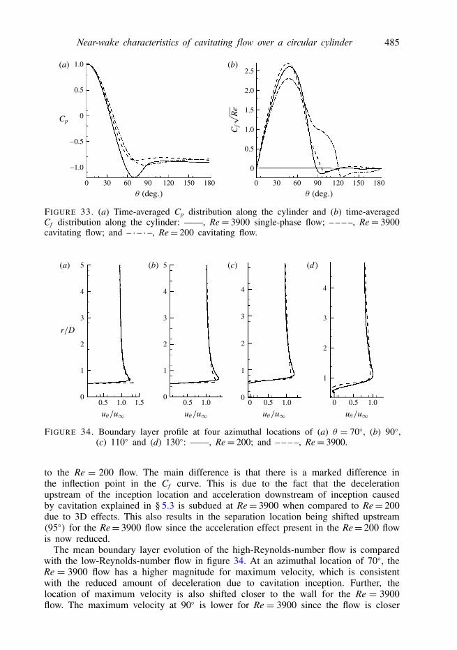
FIGURE 32. (Colour online) Mean void fraction contour for (a) Re = 3900 and(b) Re= 200.

in the vortices for the laminar case. The length of the cavity (lcav/D) is 3.04 for thehigh-Reynolds-number flow, while it is only 2.71 for the low-Reynolds-number flow.Also note the presence of a larger fraction of vapour in the wake for Re= 3900. Thusincreasing Reynolds number at the same cavitation number makes the flow cavitatemore, resulting in a larger cavity dimension. This observation is also in line with thatof Rao & Chandrasekhara (1976). The presence of an increased amount of vapour alsoaffects the Cp and Cf distributions. Figure 33(a,b) compares the time-averaged Cp andCf distributions of Re= 3900 at σ = 1.0 with the Re= 200 flow at the same cavitationnumber. Also shown in the figure are the Cp and Cf distributions from the single-phaseflow at Re= 3900, which will be discussed in § 7.2. When compared to the Re= 200flow, the minimum Cp location is shifted upstream, pointing to the inception locationmoving upstream. The magnitude of the minimum Cp is also reduced in the Re=3900flow, which is also consistent with the increased amount of vapour. The Cf curvefor the Re = 3900 flow in figure 33(b) shows a different behaviour when compared


30 60 90 120 150 1800 30 60 90 120 150 1800

0.5

0

–0.5

–1.0

1.0

0.5

0

1.0

1.5

2.0

2.5(a) (b)

FIGURE 33. (a) Time-averaged Cp distribution along the cylinder and (b) time-averagedCf distribution along the cylinder: ——, Re= 3900 single-phase flow; – – – –, Re= 3900cavitating flow; and – · – · –, Re= 200 cavitating flow.

0

1

2

3

4

5

0

1

2

3

4

5

0

1

2

3

4

1

2

3

4

0.5 1.0 1.5 0.5 1.0 0 0.5 1.0 0 0.5 1.0

(a) (b) (c) (d )

FIGURE 34. Boundary layer profile at four azimuthal locations of (a) θ = 70, (b) 90,(c) 110 and (d) 130: ——, Re= 200; and – – – –, Re= 3900.

to the Re = 200 flow. The main difference is that there is a marked difference inthe inflection point in the Cf curve. This is due to the fact that the decelerationupstream of the inception location and acceleration downstream of inception causedby cavitation explained in § 5.3 is subdued at Re= 3900 when compared to Re= 200due to 3D effects. This also results in the separation location being shifted upstream(95) for the Re= 3900 flow since the acceleration effect present in the Re= 200 flowis now reduced.

The mean boundary layer evolution of the high-Reynolds-number flow is comparedwith the low-Reynolds-number flow in figure 34. At an azimuthal location of 70, theRe = 3900 flow has a higher magnitude for maximum velocity, which is consistentwith the reduced amount of deceleration due to cavitation inception. Further, thelocation of maximum velocity is also shifted closer to the wall for the Re = 3900flow. The maximum velocity at 90 is lower for Re = 3900 since the flow is closer


120 130 140 100 10110–1 102

100

10–6

10–12

0.5

1.0

0

–0.5

PSD

St

(a) (b)

FIGURE 35. (Colour online) (a) Lift and drag coefficient history, and (b) power spectraldensity: ——, CL; – – – –, CD.

0–1.0 –0.5 0.5 1.0

0.5

1.0

0

–0.5

–1.0

0–1.0 –0.5 0.5 1.0

0.5

1.0

0

–0.5

–1.0

–1.0 0.2–0.2 0.6–0.6 –5.0 1.0 3.0 5.0–3.0 –1.0

(a) (b)

FIGURE 36. (Colour online) (a) Mean velocity divergence contour. (b) Mean vorticitydilatation contour.

to the separation point and is decelerating much more than the Re= 200 flow at thesame location. The flow separates at approximately 95 and instances of separatedflow can be observed at the downstream locations.

The lift and drag history and their power spectral density are plotted in figure 35.The secondary peaks due to pressure wave impingement are not as prominent as theywere in the Re=200 flow. The presence of an increased amount of vapour in the wakepresumably reduces the effect of pressure wave impingement. The Strouhal numbercorresponding to vortex shedding frequency is 0.167, and the reason for the Strouhalnumber reduction from the single-phase value of 0.2 is very similar to that for the 2Dflow and is depicted in figure 36(a,b). The mean velocity divergence contour shows anexpansion region corresponding to vapour formation. A compression region is foundimmediately downstream of the expansion similar to the Re= 200 flow. The expansionregion causes vorticity dilatation that can be observed in figure 36(b). As in the Re=200 flow, this vorticity dilatation is the main reason for the vorticity reduction whichreduces the vortex shedding frequency.


1 2 3

0 1 2 31 2 3

0.5

0

–0.5

–1.0

–1.5

1.0

0.5

0

1.0

0 0.5 1.0 1.5 2.0 2.5 3.0

0.5

0

–0.5

–1.0

–1.5

–2.0

–2.5

0

–0.1

–0.2

0.1

–0.3

(a) (b)

(c) (d )

FIGURE 37. Comparison of vertical profiles at streamwise stations downstream of thecylinder at Re= 3900:u, Verma & Mahesh (2012); ——, present results.

7.2. Comparison of Re= 3900 cavitating flow to Re= 3900 non-cavitating flowFigure 35(a,b) also compares the Cp and Cf distributions of Re= 3900 cavitating flowwith that of the single-phase results of Verma & Mahesh (2012) at the same Reynoldsnumber. Cavitation decreases the magnitude of minimum Cp when compared to thesingle-phase Cp and the flattening of the Cp curve is due to the presence of vapour,similar to the discussion in § 5.1. The Cf curve comparison shows that the separationlocation is shifted downstream compared to the single-phase flow. The reason for thisshift is the same as discussed in § 5.3.

Figures 37 and 38 compare the mean velocity profiles and turbulence intensityprofiles, respectively, in the wake for the cavitating case at Re = 3900 to thesingle-phase results of Verma & Mahesh (2012) at the same Reynolds number.The streamwise velocity profiles at all stations show a wider wake profile for thecavitating flow. The station x/D= 3.0 shows the maximum difference in the verticalvelocity profile since it corresponds to the cavity closure region. Inside the cavity(except at x/D= 1.06), larger values of vertical velocity are obtained. The maximumvalue for u′u′ occurs downstream (x/D = 3.0), pointing to a larger formation length.Inside the cavity, the values for v′v′ are much smaller than those obtained for thesingle-phase flow. However, the cavity closure at x/D = 3.0 is highly unsteady withhigher fluctuation values in both streamwise and vertical velocities. The u′v′ curveshows a similar trend to the mean vertical velocity profiles. Overall, cavitation seems


0

–0.2

–0.4

0.2

0.4

0

–0.2

–0.4

0.2

0.05

–0.1

–0.15

0

–0.6

0.6

0

–0.2

–0.4

–0.6

0

–0.2

–0.4

–0.6

–0.8

0

–0.1

0.1

0.2

(a) (b) (c)

(d ) (e) ( f )

0 01 2 3 1 2 3 1 2 3

1 2 3 1 2 3 1 2 3

0

0

FIGURE 38. Comparison of vertical profiles at streamwise stations downstream of thecylinder at Re= 3900:u, Verma & Mahesh (2012); ——, present results.

2

4

0

–2

–4

2

4

0

–2

–40 5 10 0 5 10

0 1.07 2.14 3.21 4.29 0 1.12 2.24 3.37 4.49

(a) (b)

FIGURE 39. (Colour online) Magnitude of vortex stretching in the symmetry plane for(a) cavitating flow and (b) non-cavitating flow.

to have delayed the complete 3D breakdown of the Kármán vortices by effectivelylowering the Reynolds number in the wake. This fact is corroborated in figure 39,which shows the instantaneous magnitude of vortex stretching in the symmetryplane for the multiphase and single-phase flows. Note that the vortex stretchingmagnitude in the wake is reduced in a cavitating flow. Hence formation of vapoursuppresses turbulence, yielding highly correlated spanwise structures in the near wakein figure 30.

8. Summary

A numerical method based on the homogeneous mixture model and characteristic-based filtering is used to study cavitation on a circular cylinder at two Reynoldsnumbers and several cavitation numbers. The simulated cavitation numbers correspond


to two different regimes based on how the cavity is shed into the wake. Thedynamics of cavity formation and collapse leading to pressure waves is capturedin the simulations and discussed in detail. A scaling for cavitation number basedon maximum velocity in the shear layer is found to collapse the cavity length as afunction of cavitation numbers at different Reynolds numbers onto a single curve. Inthe cyclic regime (σ = 1.0) of cavitation, the cavity detaches from the body itselfat the shedding frequency, while in the transitory regime of cavitation (σ = 0.7 and0.5), a low-frequency cavity detachment phenomenon is observed in addition to theshedding frequency. Cavitation is found to significantly modify the vortex sheddingfrequency, and vorticity dilatation due to vapour is found to be responsible for thisshedding frequency reduction. This effect is further verified by computing circulationin the wake, which shows that vorticity reduces as the cavitation number is lowered.

The effect of initial void fraction is assessed. It is found that changing the initialvoid fraction does not affect the general dynamics of cavity formation. However, thespeed of sound is altered significantly and this leads to pressure waves travellingat different speeds. The compressibility and acoustic impedance of the medium arealtered but the condensation ratio in the medium shows a similarity for differentfree-stream void fraction values. The pressure fluctuation contours show spatiallylocal phenomenon due to the interaction between condensation waves and vortices atspecific locations in space.

Finally, LES of cavitating flow at Re = 3900 reveals that the length of the meancavity obtained at higher Reynolds number is higher than that at low Reynoldsnumber for the same cavitation number. The vortex shedding frequency is againlower compared to a single-phase shedding frequency and vorticity dilatation is againfound to be an important factor in reducing the vorticity in the wake. Cavitationeffectively reduces the Reynolds number in the near wake, suppresses turbulence anddelays the 3D breakdown of Kármán vortices.

AcknowledgementsThis work was supported by the United States Office of Naval Research under

ONR grant N00014-11-1-0497 with Dr K.-H. Kim as technical monitor. Computingresources were provided by the Arctic Region Supercomputing Center of HPCMP andthe Minnesota Supercomputing Institute.

REFERENCES

ARAKERI, V. H. 1975 Viscous effects on the position of cavitation separation from smooth bodies.J. Fluid Mech. 68 (4), 779–799.

ARAKERI, V. H. & ACOSTA, A. J. 1973 Viscous effects in the inception of cavitation on axisymmetricbodies. Trans. ASME J. Fluids Engng 95 (4), 519–527.

ARNDT, R. E. A. 2002 Cavitation in vortical flows. Annu. Rev. Fluid Mech. 34 (1), 143–175.ARNDT, R. E. A. & MAINES, B. H. 2000 Nucleation and bubble dynamics in vortical flows. Trans.

ASME J. Fluids Engng 122 (3), 488–493.ARNDT, R. E. A., SONG, C. C. S., KJELDSEN, M., HE, J. & KELLER, A. 2000 Instability of

partial cavitation: a numerical/experimental approach. In Proceedings of the 23rd Symposiumon Naval Hydrodynamics, pp. 519–615. National Academies Press.

BALACHANDAR, R. & RAMAMURTHY, A. S. 1999 Pressure distribution in cavitating circular cylinderwakes. J. Engng Mech. 125 (3), 356–358.

BEARMAN, P. W. 1969 On vortex shedding from a circular cylinder in the critical Reynolds numberregime. J. Fluid Mech. 37 (3), 577–585.


BELAHADJI, B., FRANC, J.-P. & MICHEL, J.-M. 1995 Cavitation in the rotational structures of aturbulent wake. J. Fluid Mech. 287, 383–403.

BRANDNER, P. A., WALKER, G. J., NIEKAMP, P. N. & ANDERSON, B. 2010 An experimentalinvestigation of cloud cavitation about a sphere. J. Fluid Mech. 656, 147–176.

COLONIUS, T. 2004 Modeling artificial boundary conditions for compressible flow. Annu. Rev. FluidMech. 36, 315–345.

COUTIER-DELGOSHA, O., STUTZ, B., VABRE, A. & LEGOUPIL, S. 2007 Analysis of cavitating flowstructure by experimental and numerical investigations. J. Fluid Mech. 578, 171–222.

DIPANKAR, A., SENGUPTA, T. K. & TALLA, S. B. 2007 Suppression of vortex shedding behind acircular cylinder by another control cylinder at low Reynolds numbers. J. Fluid Mech. 573,171–190.

FRANC, J.-P. & MICHEL, J.-M. 1985 Attached cavitation and the boundary layer: experimentalinvestigation and numerical treatment. J. Fluid Mech. 154, 63–90.

FRANC, J.-P. & MICHEL, J.-M. 1988 Unsteady attached cavitation on an oscillating hydrofoil.J. Fluid Mech. 193, 171–189.

FRY, S. 1984 Investigating cavity/wake dynamics for a circular cylinder by measuring noise spectra.J. Fluid Mech. 142, 187–200.

GERRARD, J. H. 1966 The mechanics of the formation region of vortices behind bluff bodies.J. Fluid Mech. 25 (2), 401–413.

GNANASKANDAN, A. & MAHESH, K. 2014 Large eddy simulation of sheet to cloud cavitation. InProceedings of the 30th Symposium on Naval Hydrodynamics, pp. 1–13.

GNANASKANDAN, A. & MAHESH, K. 2015 A numerical method to simulate turbulent cavitatingflows. Intl J. Multiphase Flow 70, 22–34.

HAMMACHE, M. & GHARIB, M. 1991 An experimental study of the parallel and oblique vortexshedding from circular cylinders. J. Fluid Mech. 232, 567–590.

HSIAO, C.-T. & CHAHINE, G. L. 2005 Scaling of tip vortex cavitation inception noise with a bubbledynamics model accounting for nuclei size distribution. Trans. ASME J. Fluids Engng 127(1), 55–65.

KATZ, J. 1982 Cavitation inception in seperated flows. PhD thesis, California Institute of Technology.KATZ, J. 1984 Cavitation phenomena within regions of flow separation. J. Fluid Mech. 140, 397–436.KUBOTA, A., KATO, H. & YAMAGUCHI, H. 1992 A new modelling of cavitating flows: a numerical

study of unsteady cavitation on a hydrofoil section. J. Fluid Mech. 240, 59–96.KUNZ, R. F., BOGER, D. A., STINEBRING, D. R., CHYCZEWSKI, T. S., LINDAU, J. W., GIBELING,

H. J., VENKATESWARAN, S. & GOVINDAN, T. R. 2000 A preconditioned Navier–Stokesmethod for two-phase flows with application to cavitation prediction. Comput. Fluids 29 (8),849–875.

LABERTEAUX, K. R. & CECCIO, S. L. 2001 Partial cavity flows. Part 1. Cavities forming on modelswithout spanwise variation. J. Fluid Mech. 431, 1–41.

MATSUDAIRA, Y., GOMI, Y. & OBA, R. 1992 Characteristics of bubble-collapse pressures in aKarman-vortex cavity. JSME Intl J. 35 (2), 179–185.

MITTAL, S. & RAGHUVANSHI, A. 2001 Control of vortex shedding behind circular cylinder for flowsat low Reynolds numbers. Intl J. Numer. Meth. Fluids 35 (4), 421–447.

PARK, N. & MAHESH, K. 2007 Numerical and modeling issues in LES of compressible turbulenceon unstructured grids. In Proceedings of the 45th AIAA Aerospace Sciences Meeting andExhibit, AIAA Paper, pp. 1–18.

RAMAMURTHY, A. S. & BHASKARAN, P. 1977 Constrained flow past cavitating bluff bodies. Trans.ASME J. Fluids Engng 99 (4), 717–726.

RAO, B. C. S. & CHANDRASEKHARA, D. V. 1976 Some characteristics of cavity flow past cylindricalinducers in a venturi. Trans. ASME J. Fluids Engng 98 (3), 461–466.

RAO, B. C. S., CHANDRASEKHARA, D. V. & SEETHARAMIAH, K. 1972 A high-speed photographicstudy of vortex shedding behind circular cylinders of cavitating flows. In Proceedings of 2ndInternational JSME Symposium Fluid Machinery and Fluidics, pp. 293–302.

ROSHKO, A. 1961 Experiments on the flow past a circular cylinder at very high Reynolds number.J. Fluid Mech. 10 (3), 345–356.


ROUSE, H. & MCNOWN, J. S. 1948 Cavitation and pressure distribution: head forms at zero angleof yaw. State University of Iowa, Studies in Engineering, Bulletin 32. Published by the StateUniversity of Iowa.

SAITO, Y. & SATO, K. 2003 Cavitation bubble collapse and impact in the wake of a circular cylinder.In Proceedings of the 5th International Symposium on Cavitation, pp. 1–6.

SAITO, Y., TAKAMI, R., NAKAMORI, I. & IKOHAGI, T. 2007 Numerical analysis of unsteady behaviorof cloud cavitation around a NACA0015 foil. Comput. Mech. 40 (1), 85–96.

SCHMIDT, S. J., SCHNERR, G. & THALHAMER, M. 2009 Inertia controlled instability and small scalestructures of sheet and cloud cavitation. In Proceedings of the 7th International Symposiumon Cavitation, pp. 1–14.

SCHNERR, G. H., SEZAL, I. H. & SCHMIDT, S. J. 2008 Numerical investigation of three-dimensionalcloud cavitation with special emphasis on collapse induced shock dynamics. Phys. Fluids 20(4), 1–9.

SELIM, S. M. 1981 Cavitation erosion in fluid flow. PhD thesis, University of Southampton.SENOCAK, I. & SHYY, W. 2002 A pressure-based method for turbulent cavitating flow computations.

J. Comput. Phys. 176 (2), 363–383.SEO, J. H., MOON, Y. J. & SHIN, B. R. 2008 Prediction of cavitating flow noise by direct numerical

simulation. J. Comput. Phys. 227 (13), 6511–6531.SHIN, B. R., IWATA, Y. & IKOHAGI, T. 2003 Numerical simulation of unsteady cavitating flows

using a homogenous equilibrium model. Comput. Mech. 30 (5–6), 388–395.SINGHAL, A. K., ATHAVALE, M. M., LI, H. & JIANG, Y. 2002 Mathematical basis and validation

of the full cavitation model. Trans. ASME J. Fluids Engng 124 (3), 617–624.STRYKOWSKI, P. J. & SREENIVASAN, K. R. 1990 On the formation and suppression of vortex

shedding at low Reynolds numbers. J. Fluid Mech. 218, 71–107.VARGA, J. J. & SEBESTYEN, G. Y. 1972 Determination of hydrodynamic cavitation intensity by noise

measurement. In Proceedings of the 2nd International JSME Symposium on Fluid Machineryand Fluidics, pp. 285–292.

VERMA, A. & MAHESH, K. 2012 A Lagrangian subgrid-scale model with dynamic estimation ofLagrangian time scale for large eddy simulation of complex flows. Phys. Fluids 24 (8),85–101.

WILLIAMSON, C. H. K. 1988 Defining a universal and continuous Strouhal–Reynolds numberrelationship for the laminar vortex shedding of a circular cylinder. Phys. Fluids 31 (10),2742–2744.

WILLIAMSON, C. H. K. 1989 Oblique and parallel modes of vortex shedding in the wake of acircular cylinder at low Reynolds numbers. J. Fluid Mech. 206, 579–627.

YEE, H. C., SANDHAM, N. D. & DJOMEHRI, M. J. 1999 Low-dissipative high-order shock-capturingmethods using characteristic-based filters. J. Comput. Phys. 150 (1), 199–238.

YOUNG, J. O. & HOLL, J. W. 1966 Effects of cavitation on periodic wakes behind symmetricwedges. Trans. ASME J. Fluids Engng 88 (1), 163–176.

Documents

J. Fluid Mech. (2016), . 790, pp. doi:10.1017/jfm.2016.19 ...kmahesh/globalassets/publpdf/journal/aswin_jfm... · Key words: cavitation, vortex dynamics, wakes ... The objective of