J. Fluid Mech. (2014), . 742, doi:10.1017/jfm.2013.651 ... · J. Fluid Mech. (2014), ... Stochastic dynamics of active swimmers in linear ˛ows Mario Sandoval1,2,†, Navaneeth K

J. Fluid Mech. (2014), vol. 742, pp 50–70. c© Cambridge University Press 2014doi:10.1017/jfm.2013.651

50

Stochastic dynamics of active swimmers inlinear flows

Mario Sandoval1,2,†, Navaneeth K. Marath3, Ganesh Subramanian3 andEric Lauga1,4

1Department of Mechanical and Aerospace Engineering, University of California San Diego,9500 Gilman Drive, La Jolla, CA 92093-0411, USA

2Department of Physics, Universidad Autonoma Metropolitana-Iztapalapa, Apartado Postal 55-534,Mexico, Distrito Federal 09340, Mexico

3Engineering Mechanics Unit, JNCASR, Bangalore 560064, India4Department of Applied Mathematics and Theoretical Physics, University of Cambridge,

Centre for Mathematical Sciences, Wilberforce Road, Cambridge CB3 0WA, UK

(Received 2 November 2012; revised 10 October 2013; accepted 9 December 2013)

Most classical work on the hydrodynamics of low-Reynolds-number swimmingaddresses deterministic locomotion in quiescent environments. Thermal fluctuations influids are known to lead to a Brownian loss of the swimming direction, resulting in atransition from short-time ballistic dynamics to effective long-time diffusion. As mostcells or synthetic swimmers are immersed in external flows, we consider theoreticallyin this paper the stochastic dynamics of a model active particle (a self-propelledsphere) in a steady general linear flow. The stochasticity arises both from translationaldiffusion in physical space, and from a combination of rotary diffusion and so-calledrun-and-tumble dynamics in orientation space. The latter process characterizes themanner in which the orientation of many bacteria decorrelates during their swimmingmotion. In contrast to rotary diffusion, the decorrelation occurs by means of large andimpulsive jumps in orientation (tumbles) governed by a Poisson process. We beginby deriving a general formulation for all components of the long-time mean squaredisplacement tensor for a swimmer with a time-dependent swimming velocity andwhose orientation decorrelates due to rotary diffusion alone. This general frameworkis applied to obtain the convectively enhanced mean-squared displacements of asteadily swimming particle in three canonical linear flows (extension, simple shearand solid-body rotation). We then show how to extend our results to the case wherethe swimmer orientation also decorrelates on account of run-and-tumble dynamics.Self-propulsion in general leads to the same long-time temporal scalings as forpassive particles in linear flows but with increased coefficients. In the particularcase of solid-body rotation, the effective long-time diffusion is the same as that ina quiescent fluid, and we clarify the lack of flow dependence by briefly examiningthe dynamics in elliptic linear flows. By comparing the new active terms with thoseobtained for passive particles we see that swimming can lead to an enhancement ofthe mean-square displacements by orders of magnitude, and could be relevant for

† Email address for correspondence: [email protected]

mailto:[email protected]

Stochastic dynamics of active swimmers in linear flows 51

biological organisms or synthetic swimming devices in fluctuating environmental orbiological flows.

Key words: biological fluid dynamics, shear flows, low-Reynolds number locomotion

1. IntroductionA complete physical understanding of many processes occurring at small scales

and involving active particles has proven both challenging and an exciting avenue forbiomechanics and bioengineering research. Important biological topics with ongoingresearch include the dynamics of plankton in marine ecosystems (Guasto, Rusconi &Stocker 2012), the collective behaviour of dense micro-organism suspensions (Koch& Subramanian 2011) and their appendages (Lauga & Goldstein 2012), and theinteractions between swimming cells and complex environments (Lauga & Powers2009). In the bioengineering world, the focus is on the design of effective, andpractical synthetic locomotion systems able to carry out future detection, diagnosisand treatment of diseases (Paxton et al. 2006; Abbott et al. 2009; Mallouk & Sen2009; Mirkovic et al. 2010).

Focusing on the dynamics of a single active particle or self-propelled cell, mostclassical work considered the kinematics and energetics of deterministic locomotionin a quiescent fluid. Owing to their small sizes, many swimming cells, in particular,bacteria and small single-cell eukaryotes, as well as many synthetic swimmers, areexpected to have their swimming direction affected by thermal fluctuations (Lovely& Dahlquist 1975; Pedley & Kessler 1992; Berg 1993; Ishikawa & Pedley 2007;Howse et al. 2007; ten Hagen, van Teeffelen & Lowen 2009, 2011a; Lauga 2011).Even for bacteria large enough to not be Brownian, there continue to be stochasticfluctuations in orientation that are largely athermal in origin. For instance, for abacterium Escherichia coli during a swimming run, the observed rate of orientationdecorrelation is one order of magnitude faster than that predicted based on a rotaryBrownian diffusivity (Berg 1993), and is likely due to shape fluctuations of theimperfect bundle of bacterial flagella (Locsei & Pedley 2009; Subramanian & Koch2009; Koch & Subramanian 2011).

Furthermore, in most situations of biological or applied interest, self-propelledorganisms and synthetic swimmers are subject to external flows, for example planktontransported by small-scale turbulence, bacteria in the initial stages of environmentalbiofilm formation or swimming through human organs. Similarly, any future practicalimplementation of artificial micron-scale swimmers will have to be able to navigatethrough flowing bodily fluids, in particular the bloodstream (Abbott et al. 2009; Kosaet al. 2012; Wang & Gao 2012).

Previous classical studies have addressed the effect of external flows on Brownianmotion of passive spherical colloids, most notably in simple shear (San-Miguel &Sancho 1979; Subramanian & Brady 2004) and for the more general case of anarbitrary incompressible linear flow (Foister & van de Ven 1980). For a passivespherical Brownian particle in a linear flow, the long-time diagonal element of itsmean-square displacement dyadic along the flow direction is proportional to thethird power of time in the case of simple shear, grows at an exponential rate (alongthe extensional axis) in the case of pure extensional flow, but continues to displaya diffusive scaling in the case of solid-body rotation. In the case of a shear flow,

52 M. Sandoval, K. N. Marath, G. Subramanian and E. Lauga

Clercx & Schram (1992) studied a similar problem based on the time-dependentlinearized Navier–Stokes equations, instead of the Stokes equations, in order toaddress the non-trivial modifications in the short-time dynamics arising from theinclusion of fluid inertial effects. The analogous situation in the absence of a flow isclassical work (Hinch 1975; Zwanzig & Bixon 1970; Hauge & Martin-Löf 1973), andaccounting for the finite time scale on which vorticity diffuses leads to an algebraic(rather than exponential) decay in the relevant correlations. For non-spherical particles,the dynamics cannot in general be obtained in closed form, since the translationaldispersion is intimately coupled to the orientation distribution, and the latter cannotbe determined analytically for arbitrary values of the rotary Péclet number (Frankel& Brenner 1991, 1993). Asymptotic analysis is, however, possible both for smallvalues of the rotary Péclet number (Brenner 1974; Brenner & Condiff 1974) and inthe limit of weak Brownian motion (Leal & Hinch 1971).

The dynamics of active particles in shearing flows has been addressed in recentstudies. Jones, Baron & Pedley (1994) calculated, in the absence of noise, thedirection of swimming of bottom-heavy micro-organisms immersed in shear flows.Bearon & Pedley (2000) modelled a spherical chemotactic bacterium and derivedan advection–diffusion equation for the cell density which included the influence ofshear. Locsei & Pedley (2009) addressed the run-and-tumble dynamics of bacteriaand the effect of a shear flow on the chemotaxis response of the cell. More recently,ten Hagen, Wittkowski & Lowen (2011b) characterized, in two spatial dimensions,the dynamics of a spherical self-propelled particle in a shear flow and subject to anexternal torque, and obtained an enhancement of the ∼t3 mean-square dynamics. Theeffect of an external linear flow on the rheology of, and the pattern formation by,suspensions of active particles was considered by Rafai, Jibuti & Peyla (2010) andSaintillan (2010a,b), Pahlavan & Saintillan (2011).

In this paper we quantify the interplay between fluctuations (thermal or otherwise)and a prototypical external flow, namely a steady, incompressible linear flow, on thedynamics of an active particle. The particle is assumed to be spherical, a geometryrelevant to many biological and bioengineering situations, including the dynamics ofself-catalytic colloidal spheres (Golestanian, Liverpool & Ajdari 2007; Howse et al.2007; Jülicher & Prost 2009; Brady 2010), active droplets (Thutupalli, Seemann& Herminghaus 2011; Schmitt & Stark 2013) and the alga Volvox (Drescher et al.2009). The activity of the particle, which is free to move in three spatial dimensions,is modelled as a prescribed swimming velocity in its body frame. We first develop theanalysis in the case where the particle is subject to both rotational and translationalBrownian motion, in addition to being convected by the ambient linear flow. Wethen extend the results to include the biologically relevant reorientation mechanismassociated with the run-and-tumble dynamics exhibited by many bacteria (Berg 1993,2004). We ignore other potentially relevant reorientation mechanisms, including phaseslips which occur between the pair of anterior flagella of the Chlamydomonas algae(Polin et al. 2009), hydrodynamically mediated collisions that govern the dynamicsat high volume fraction (Ishikawa & Pedley 2007) and run-and-reverse dynamics(Guasto et al. 2012).

After setting up the problem in § 2, we derive in § 3, by means of an elementaryrotational transformation, the transition probability density for a particle whoseorientation evolves on account of a rotary diffusion process. We then use thisprobability density to find all components of the swimming direction correlationmatrix. We exploit these results to calculate the general expression for the mean-square displacement dyadic of the active particle in § 4 and evaluate each of its


components analytically in the specific case of an active particle undergoing steadyswimming in § 5. In the absence of external flow, or for passive particles, ouranalytical results recover the well-known classical limits. By focusing on threeprototypical flows (simple shear, extension and solid-body rotation) in § 6, wedemonstrate that the particle activity does not modify the long-term temporal scalingsfor the mean-square displacements, but increases its coefficients in the case of shearand extension while the results are unchanged in the case of solid-body rotation. In§ 7, we extend the analysis to include an additional intrinsic orientation decorrelationmechanism, namely that associated with correlated tumbles, the occurrence of whichis modelled as a Poisson process. We demonstrate that the effect of tumbles may besimply incorporated as an additive contribution to the rate of orientation decorrelation,and the results already obtained may therefore be readily extended to includeswimmers whose orientation evolves due to both rotary diffusion and run-and-tumbledynamics. We close by offering a physical discussion of our results in § 8 usingscaling arguments. In particular, we explain the singular flow-independent nature ofsolid-body rotation by considering the behaviour of the mean-squared displacementin elliptic linear flows (i.e. two-dimensional linear flows with closed streamlines),and examining its dependence on the ratio of the ambient vorticity to extension.Comparing the coefficients in the active versus passive case, we see that swimmingcan lead to enhancement of the mean-square dynamics by orders of magnitude, aresult which could be relevant for both biology and bioengineering.

2. A spherical active particle in an incompressible linear flowWe consider a spherical particle of radius a that self-propels (swims) in a three-

dimensional fluctuating environment and in the presence of a general linear externalflow. In the absence of noise and external flow, we assume that the particle swimsat the intrinsic velocity Us(t), prescribed in the body frame of the particle. We usea Cartesian coordinate system with vectors i, j, k and corresponding coordinates(x1, x2, x3). The external flow, U∞, is assumed to be any general two-dimensionallinear, incompressible flow of the form U∞ = (Gx2, αGx1, 0), with G > 0 denotingthe deformation rate. The particle orientation is described by the angles (θ, ϕ) ina spherical coordinates system, where θ and ϕ are the polar and azimuthal angles,respectively. The dimensionless parameter α allows us to tune the type of externalflow considered, from pure rotation (α = −1) to shear (α = 0) and extensional flow(α = 1).

The over-damped balance of forces and torques on the particle leads to theBrownian dynamics equations determining its instantaneous translational velocity,U(t), and angular velocity, Ω(t), as solutions to

RU(U −Us −U∞)= f , RΩ (Ω −Ω∞)= g, (2.1)

where Ω∞ = ωαk, with ωα = (G/2)(α − 1), is the angular velocity of the particleinduced by the general linear flow. In (2.1), RU =RU I and RΩ =RΩ I are the viscousresistance coefficients (RU = 6πηa and RΩ = 8πηa3 in a Newtonian fluid of shearviscosity η) and I is the unit tensor. The vectors f and g represent zero-meanBrownian random forces and torques whose correlations in their components aregoverned by the fluctuation–dissipation theorem as

〈fi(t)fj(t′)〉 = 2kBTRUδijδ(t− t′), 〈gi(t)gj(t′)〉 = 2kBTRΩδijδ(t− t′), (2.2)

with 〈·〉 representing ensemble averaging (Doi & Edwards 1999).


Denoting the particle location as x (t)= (x1(t), x2(t), x3(t))T, the equation governingx (t), from (2.1), can be formally written as

dxdt=Mx(t)+Us(t)e(t)+ f (t), M=

0 G 0αG 0 00 0 0

, (2.3)

where e(t) = (e1(t), e2(t), e3(t))T is a unit vector pointing in the instantaneousswimming direction of the particle, Us(t) the magnitude of the instantaneousswimming velocity along e(t) (in other words, Us(t) = Us(t)e(t)), and f ≡ R−1

U f .Similarly, the director vector, e, follows the dynamics (Coffey, Kalmikov & Valdron1996)

dedt= [ωαk+ g(t)

]× e(t), (2.4)

where g≡ R−1Ω g.

In the stochastic system of equations (2.3)–(2.4), the equation for the particleorientation, (2.4), can be solved first and its solution can then be used in (2.3) toobtain the particle position. In order to determine all components of the symmetricmean-square displacement tensor, 〈x(t)x(t)T〉, we therefore first have to compute allcomponents of the orientation correlation matrix.

3. Rotational probability distribution function and orientation correlations

The orientation correlation matrix, 〈e(t)e(0)T〉, can be evaluated if we know theorientation transition probability distribution function (p.d.f.), P(e, t|e0, 0), withe(0)≡ e0, governing the swimmer orientation, e(t). Since the angular velocity of thespherical swimmer is along the k-axis, to determine P we apply to (2.4), a rotationaltransformation around the k direction of the frame fixed at the particle centre, namely

e(t)=R(t)e′(t), R(t)=

cosωαt − sinωαt 0sinωαt cosωαt 0

0 0 1

, (3.1)

where e′(t) is the orientation vector in a coordinate system rotating with the flowvorticity. This transformation reduces (2.4) to de′/ dt = g′(t)× e′(t), whose p.d.f. forthe director vector is classically given by an infinite sum over spherical harmonics(Berne & Pecora 2000). The transformation between the fixed and rotating framesof reference, in a spherical coordinate system with its polar axis along the ambientvorticity, only involves the two azimuthal angles (ϕ′ = ϕ − ωαt, ϕ and ϕ′ are theazimuthal angles for fixed and rotating frames of references, respectively). Substitutingthis transformation, we find the required p.d.f. of the director, P, in a general linearflow as

P(e, t|e0, 0)=∞∑

l=0

l∑

m=−l

e−DΩ l(l+1)tYm∗l (θ0, ϕ0) Ym

l (θ, ϕ) e−imωα t, (3.2)

where Yml are the spherical harmonics (Abramowitz & Stegun 1970), Ym∗

l theircomplex conjugates, and θ0 and ϕ0 are the polar and azimuthal angles for e0. In(3.2), DΩ is the rotary diffusivity for the particle. When it has a thermal origin, itis determined in terms of the amplitude of the Brownian force correlation (see (2.2)),


and is given by kBT/RΩ . The underlying random fluctuations in orientation may notbe Brownian, however, in which case DΩ may be directly inferred from the observedrate of change of the mean square angular displacement (Berg 1993). With the explicitexpression for the p.d.f. known, the correlation matrix for the swimming orientationmay then be evaluated. The ijth component is given by

⟨ei(t)ej(0)

⟩=∫

d2e0

∫d2e ei(t)ej(0)G(e, t; e0, 0), (3.3)

where i, j are in 1,2,3, and where G(e, t; e0, 0) is the joint p.d.f. for the directorvector with orientation e0 at time t= 0 and orientation e(t) at time t (Berne & Pecora2000). For an assumed isotropic distribution of orientation at the initial instant, thisjoint probability is given by the product of the uniform p.d.f. for e0 (1/4π) withthe transition p.d.f. (P) for the orientation vector e(t), given that we know that theorientation was e0 at t= 0 and thus we have

G(e, t; e0, 0)= 14π

P(e, t|e0, 0). (3.4)

Using this formalism, all components of 〈e(t)e(0)T〉 may be systematically obtained.For example, for i= 1 and j= 2, solving (3.3) directly leads to

〈e1(t)e2(0)〉 = 14π

∞∑

l=0

l∑

m=−l

e−DΩ l(l+1)te−imωα tDml , (3.5)

where

Dml = (−1)m

∫ ∫h1 dθ0 dϕ0

∫ ∫h2 dθ dϕ, (3.6)

h1 = sin2 θ0 sin ϕ0Y−ml (θ0, ϕ0) , h2 = sin2 θ cos ϕYm

l (θ, ϕ). (3.7)

By orthogonality, we can show that Dml = 0 if l 6= 1, and by explicitly evaluating the

coefficients Dm1 we get

〈e1(t)e2(0)〉 =− 13 e−2DΩ t sinωαt. (3.8)

All other components of the orientation correlation matrix, 〈e(t)e(0)T〉, can be obtainedsimilarly, leading to the final result

⟨e(t)e(0)T

⟩= 13

e−2DΩ t


0 0 1

. (3.9)

In the plane of the linear flow, the components of the orientation correlation matrixfollow an exponential decay modulated by a harmonic function with frequency equalto the linear flow-induced rotation rate. Note that upon setting ωα = 0 in (3.9), werecover the classical exponential decay in orientation direction from Brownian motionin the absence of flow, 〈ei(t)ei(0)〉 = e−2DΩ t (Doi & Edwards 1999).

4. Mean-square displacement tensorWe now turn to determining the general formula for the mean-square displacement

dyadic, i.e. the symmetric tensor 〈x(t)x(t)T〉. An integration of (2.3) with initial


condition x(0)= 0 leads to the formal solution

x(t)=∫ t

0Us(t′)eM(t−t′)e(t′) dt′ +

∫ t

0eM(t−t′) f (t′) dt′. (4.1)

Using the definition of the exponential matrix, one can show that

eM(t−t′) =

cosh[√αG(t− t′)

] 1√α

sinh[√αG(t− t′)

]0

√α sinh

[√αG(t− t′)

]cosh

[√αG(t− t′)

]0

0 0 1

≡

b11 b12 0b21 b22 00 0 1

.

(4.2)

We start by computing the diagonal elements of 〈x(t)x(t)T〉. In order to do so weremark that, if β denotes one component of the particle position, β = xi, then

d 〈β(t)β(t)〉dt

= 2⟨β

dβdt

⟩. (4.3)

With the initial condition β(0) = 0, equation (4.3) can be integrated once to obtainexactly

〈β(t)β(t)〉 = 2∫ t

0

⟨β

dβdt

⟩dt. (4.4)

We then proceed to perform the multiplications on the right-hand side of (4.3) appliedto each of the three components of x(t) given by (4.1) and (4.2). After using thefluctuation–dissipation theorem stating that 〈fi(t)fj(t′)〉 = 2DBδ(t − t′), where DB isthe Brownian diffusion constant, DB = kBT/RU, and using that the random force andswimming direction are not correlated we obtain

⟨x1(t)

dx1

dt(t)⟩= G

∫ t

0Us(t′)b1k(t, t′)

∫ t

0Us(t2)b2l(t, t2)

⟨ek(t′)el(t2)

⟩dt2 dt′

+G∫ t

0b1l(t, t′)

∫ t

0b2k(t, t2)

⟨fl(t′)fk(t2)

⟩dt2 dt′

+Us(t)∫ t

0Us(t2)b1l(t, t2) 〈e1(t)el(t2)〉 dt2 +DB, (4.5)

⟨x2(t)

dx2

dt(t)⟩= αG

∫ t


∫ t

0Us(t2)b2l(t, t2)

⟨ek(t′)el(t2)

⟩dt2 dt′

+αG∫ t

0b1l(t, t′)

∫ t

0b2k(t, t2)

⟨fl(t′)fk(t2)

⟩dt2 dt′

+Us(t)∫ t

0Us(t2)b2l(t, t2) 〈e2(t)el(t2)〉 dt2 +DB, (4.6)

⟨x3(t)

dx3

dt(t)⟩= Us(t)

∫ t

0Us(t′)

⟨e3(t)e3(t′)

⟩dt′ +DB, (4.7)

where k, l are in 1, 2 (Einstein summation notation).In order to compute the off-diagonal elements of 〈x(t)x(t)T〉 we directly use the

integration in (4.1)–(4.2) which provides each component, (x1, x2, x3), of the particle


trajectory. The ensemble average of the direct multiplication of these componentstogether with the fact that random force and swimming direction are not correlatedleads to the general results

〈x1(t)x2(t)〉 =∫ t


∫ t

0Us(t2)b2l(t, t2)

⟨ek(t′)el(t2)

⟩dt2 dt′

+∫ t

0b1l(t, t′)

∫ t

0b2k(t, t2)

⟨fl(t′)fk(t2)

⟩dt2 dt′, (4.8)

〈x1(t)x3(t)〉 = 0, (4.9)〈x2(t)x3(t)〉 = 0. (4.10)

Independently of its swimming kinematics, for an active particle immersed in a two-dimensional linear flow, the correlations between the particle components in the planeof the linear flow and perpendicular to it are zero.

5. Application to steady swimmingIn the previous section, the general formulae for each component of the mean-

square displacement dyadic, 〈x(t)x(t)T〉, were derived. The final results, althoughanalytically explicit, can be quite involved if Us(t) is a complicated function of time.To get further insight into the impact of swimming on the effective particle dynamics,we apply our framework to the case of an active particle swimming in a steadyfashion, i.e. Us(t)=U, where U is a constant speed.

To illustrate how this assumption can be exploited, we consider (4.8) for thecorrelation in the cross terms of the active particle, 〈x1(t)x2(t)〉. When Us =U, usingthe fact that

∫ t

0b1l(t, t′)

∫ t

0b2k(t, t2)

⟨fl(t′)fk(t2)

⟩dt2 dt′ = 2DB

∫ t

0b1l(t, t′)b2l(t, t′) dt′, (5.1)

equation (4.8) becomes

〈x1(t)x2(t)〉 = U2∫ t

0b1k(t, t′)

∫ t

0b2l(t, t2)

⟨ek(t′)el(t2)

⟩dt2 dt′

+ 2DB

∫ t

0b1l(t, t′)b2l(t, t′) dt′. (5.2)

Using (4.2), one easily finds that

2DB

∫ t

0b1l(t, t′)b2l(t, t′) dt′ =DB

sinh2 (√αGt)

G+DB

sinh2 (√αGt)

αG. (5.3)

Furthermore, an inspection of (5.2) shows that four integrals (denoted F1–F4) have tobe evaluated, namely

F1 =U2∫ t

0b11(t, t′)

∫ t

0b21(t, t2)

⟨e1(t′)e1(t2)

⟩dt2 dt′, (5.4)

F2 =U2∫ t

0b11(t, t′)

∫ t

0b22(t, t2)

⟨e1(t′)e2(t2)

⟩dt2 dt′, (5.5)


F3 =U2∫ t

0b12(t, t′)

∫ t

0b21(t, t2)

⟨e2(t′)e1(t2)

⟩dt2 dt′, (5.6)

F4 =U2∫ t

0b12(t, t′)

∫ t

0b22(t, t2)

⟨e2(t′)e2(t2)

⟩dt2 dt′. (5.7)

In fact, one can see from the general equations (4.5)–(4.8) that the four integrals,F1–F4, together with the equality in (5.1), are common to all of the non-zerocomponents of the tensor 〈x(t)x(t)T〉 (apart from 〈x3x3〉). Evaluating F1–F4 willthus allow us to obtain explicit expressions for all components of the mean-squaredisplacement tensor.

In order to compute the first integral F1, one has to pay attention to the relativemagnitude of t2 and t′. Let us rewrite the first integral as

F1 = U2∫ t

0b11(t, t′)

[∫ t′

0b21(t, t2)

⟨e1(t′)e1(t2)

⟩dt2

+∫ t

t′b21(t, t2)

⟨e1(t2)e1(t′)

⟩dt2

]dt′, (5.8)

so that for the term in brackets we have t′> t2 in the first integral while t2 > t′ in thesecond integral. Inserting from (4.2) the corresponding values of bkl, and substitutingthe appropriate orientation correlations from (3.9) into (5.8), and after performing theintegrations we finally obtain

F1 ∼ U2√α3

A1 + A2

kαas t→∞, (5.9)

where

A1 =(a2α − b2

α + d2α − c2

α

)cosh

(√αGt

)sinh

(√αGt

)

kα, (5.10)

A2 = −2bαsinh2 (√αGt

)

2√αG

, (5.11)

with the constants aα, bα, cα, dα and kα defined as

aα =√αG(−4D2

Ω +G2α +ω2α

), (5.12)

bα = −8D3Ω + 2DΩG2α − 2DΩω

2α, (5.13)

cα = 4√αGDΩωα, (5.14)

dα = 4D2Ωωα +G2αωα +ω3

α, (5.15)

kα = 16D4Ω − 8D2

Ω

(G2α −ω2

α

)+ (G2α +ω2α

)2. (5.16)

With an identical mathematical procedure, we can solve for the other three integralterms namely (F2, F3 and F4). For F2 we find

F2 ∼ U2

3B1 + B2 + B3

kαas t→∞, (5.17)


where

B1 = 2aαcα sinh2 (√αGt)− 2bαdα cosh2 (√αGt

)

kα, (5.18)

B2 = −4DΩωα sinh2 (√αGt), B3 = 2dαbα

kα. (5.19)

For F3, we get

F3 ∼√αU2

3C1 +C2 +C3

kαas t→∞, (5.20)

where

C1 = 4DΩωα√α

sinh2 (√αGt), C2 = 1√

α

2aαcαkα

, (5.21)

C3 = 1√α

2bαdα sinh2 (√αGt)− 2aαcα cosh2 (√αGt

)

kα, (5.22)

and finally for F4 we obtain

F4 ∼ U2

3D1 +D2

kαas t→∞, (5.23)

where

D1 = −2bα√α

sinh2 (√αGt)

2√αG

, (5.24)

D2 = 1√α

(a2α − b2

α + d2α − c2

α

)sinh

(√αGt

)cosh

(√αGt

)

kα. (5.25)

In order to compute the diagonal terms in 〈x(t)x(t)T〉, we have five remainingintegrals to calculate in (4.5)–(4.7), which are constants and we have

limt→∞

U2∫ t

0b11(t, t2) 〈e1(t)e1(t2)〉 dt2 = −U2

3bαkα, (5.26)

limt→∞

U2∫ t

0b12(t, t2) 〈e1(t)e2(t2)〉 dt2 = − U2

3√α

cαkα, (5.27)

limt→∞

U2∫ t

0b21(t, t2) 〈e2(t)e1(t2)〉 dt2 = U2

3

√αcαkα

, (5.28)

limt→∞

U2∫ t

0b21(t, t2)

⟨e2(t)e2(t′)

⟩dt2 = −U2

3bαkα, (5.29)

limt→∞

U2∫ t

0

⟨e3(t)e3(t′)

⟩dt′ = U2

6DΩ

. (5.30)

Note that when α < 0, we have neglected all exponentially decaying terms in theequations above. In contrast, for α > 0, we have neglected (and therefore omitted)terms of the form e

√αGte−2DΩGt compared with those scaling as e2

√αGt in the A − D

constants, and as a result, terms such as B3 or C2, or all constants in (5.26)–(5.29),can also be neglected for α > 0.


6. Steady swimming in three different linear flowsWe computed so far the long-time components of the mean-square displacement

tensor, 〈x(t)x(t)T〉, for a particle performing steady swimming in a general two-dimensional linear flow (arbitrary value of α). In this section we apply our generalresults to the canonical cases of a solid-body rotation (α =−1), a simple shear flow(α = 0) and a pure extension (α = 1). An important dimensionless number whichwill appear compares two relevant time scales. One time scale is D−1

Ω , correspondingto the reorientation of the swimmer due to rotary diffusion (thermal or otherwise),and the other time scale is G−1, a characteristic time scale for the linear flow. Theratio between the two is a rotary Péclet number, Pe, defined as Pe ≡ G/(4DΩ)(the coefficient 4 is for mathematical convenience). Swimmers with Pe 1 willprimarily be affected by the non-hydrodynamic fluctuating forces (responsible forrotary diffusion), whereas when Pe 1 we expect the external flow to play animportant role.

6.1. Solid-body rotationIn this section we assume that the external flow is a solid-body rotation. We thensubstitute (5.1)–(5.30) into (4.5)–(4.8), and evaluate these components at α = −1.After elementary simplifications and by integrating (4.4), we obtain the analyticalexpressions for the long-time components of the mean-square displacement tensor as

〈x1(t)x1(t)〉 =(

U2

3DΩ

+ 2DB

)t, (6.1)

〈x3(t)x3(t)〉 = 〈x2(t)x2(t)〉 = 〈x1(t)x1(t)〉 , (6.2)〈x1(t)x2(t)〉 = 0. (6.3)

This result is, surprisingly, the same as the classical result for swimming-inducedenhanced effective diffusion (Lovely & Dahlquist 1975; Berg 1993). Furthermore, ifwe chose U= 0 in (6.1)–(6.3), one recovers the classical result of a Brownian passiveparticle under an external flow performing pure rotation (San-Miguel & Sancho 1979;Foister & van de Ven 1980) as

〈x1(t)x1(t)〉 = 〈x2(t)x2(t)〉 = 〈x3(t)x3(t)〉 = 2DBt, (6.4)〈x1(t)x2(t)〉 = 0. (6.5)

The fact that this result is identical to the case without any external flow will beaddressed in detail in § 8.

6.2. Simple shear flowWe now turn to the case of a simple shear flow, for which α=0. Exploiting the resultsfrom (5.1)–(5.30) to evaluate (4.5)–(4.8) at α = 0, together with (4.4), gives us theexplicit analytical expressions for the long time components of the tensor 〈x(t)x(t)T〉,namely

〈x1(t)x1(t)〉 =[

32Pe2D2ΩDB

3+ 16U2DΩ

9Pe2

1+ Pe2

]t3 + 4U2

3

[Pe4 − Pe2

(1+ Pe2

)2

]t2

+[

4U2

3DΩ

Pe2

(1+ Pe2

)2 +U2

3DΩ

(1+ Pe2

) + 2DB

]t, (6.6)


〈x2(t)x2(t)〉 =[

U2

3DΩ

(1+ Pe2

) + 2DB

]t, (6.7)

〈x3(t)x3(t)〉 =[

U2

3DΩ

+ 2DB

]t, (6.8)

〈x1(t)x2(t)〉 =[

4DΩDBPe+ 2U2

3Pe

1+ Pe2

]t2 + U2

3DΩ

[Pe3 − Pe(1+ Pe2

)2

]t, (6.9)

with the Péclet number, Pe, defined above. If we set U = 0 in (6.6)–(6.9) then ourresults reduce to those known for Brownian motion of passive particles in simple shear(San-Miguel & Sancho 1979; Foister & van de Ven 1980). We obtain

〈x1(t)x1(t)〉 = 23 G2DBt3 + 2DBt, (6.10)

〈x2(t)x2(t)〉 = 〈x3(t)x3(t)〉 = 2DBt, (6.11)〈x1(t)x2(t)〉 = GDBt2. (6.12)

The dynamics quantified by (6.6)–(6.9), which combines self-propulsion, Brownianmotion and an external simple shear flow, has a few notable features. The diagonalcomponent in the direction of the applied simple shear flow, 〈x1x1〉, is dominated, atlong time, by the O(t3) superdiffusive scaling, with a coefficient enhanced, by thepresence of swimming, above its value for passive particles. The 〈x1x1〉 componentalso includes an O(t) diffusive term, which was present for passive particles but isenhanced here by swimming, and a new intermediate O(t2) term. In contrast, thediagonal components in the directions perpendicular to the shear flow, 〈x2x2〉 and〈x3x3〉, grow linearly with time in an anisotropic fashion. The effective diffusionconstant in the shear direction, 〈x2x2〉, is always smaller than that in the vorticitydirection, 〈x3x3〉, due to shear-induced particle rotation. In both cases, swimmingincreases the effective diffusion constant above the purely Brownian diffusion constantfor passive particles. Finally, as was the case for passive Brownian motion, a non-zerocross-correlation in displacements in the plane of the flow also arises due to shear,〈x1x2〉, scaling quadratically in time, and enhanced by the presence of swimming alsoleads to a new O(t) term.

6.3. Pure extensionThe final case we analyse is that of an active particle swimming steadily in a pureextensional (irrotational) flow. Following the analysis in the previous sections we nowfind the long-time components of 〈x(t)x(t)T〉 to be given by

〈x1(t)x1(t)〉 = U2

48D2Ω

[1

Pe (1+ 2Pe)

]e2Gt + DB

8DΩPee2Gt, (6.13)

〈x2(t)x2(t)〉 = 〈x1(t)x2(t)〉 = 〈x1(t)x1(t)〉 , (6.14)

〈x3(t)x3(t)〉 =(

U2

3DΩ

+ 2DB

)t. (6.15)

Note that in order to derive the equations above we have neglected all algebraic termswhich are subdominant compared with e2Gt as long as G 6= 0. Once again, by settingU = 0 into (6.13)–(6.15), one recovers (to within exponentially small corrections) the


classical long-time correlations results of a Brownian passive particle in an extensionalflow (San-Miguel & Sancho 1979; Foister & van de Ven 1980)

〈x1(t)x1(t)〉 = 〈x2(t)x2(t)〉 = 〈x1(t)x2(t)〉 =DBG−1e2Gt/2. (6.16)

The effect of activity is to lead to the same exponential scaling as for passive particle,but with an enhanced coefficient.

7. Extension to run-and-tumble swimmersIn this section, we extend the analysis to a spherical active particle whose

orientation decorrelates due to stochastic instantaneous tumble events, in additionto the rotary diffusion process assumed above. The particle now ‘runs’, on average,in a given direction during which its orientation evolves continuously due to rotarydiffusion. However, such runs are interrupted by ‘tumbles’ that lead to large impulsivechanges in orientation. The statistics of the tumbles are well approximated by aPoisson process for the bacterium E. coli (Berg 1993). The duration of a run, trun,is therefore governed by an exponential distribution function, e−trun/τ/τ , where τ−1 isthe average tumbling frequency.

In addition to describing the temporal statistics of tumbling events, one has toprovide a model for the correlations between the pre- and post-tumble orientations.For instance, in E. coli, an average angular change of 68 per tumble has beenobserved (Berg 1993), indicative of a positive correlation. The original transitionprobability distribution introduced in § 3, P(e, t|e0, 0), is again transformed to acoordinate system rotating with the particle (e → R(t)e′, the rotation matrix R(t)being defined in § 3), and P(e′, t|e0, 0) now satisfies the equation

∂P∂t−DΩ∇2

e′P+1τ

(P−

∫K(e′|e′′)P(e′′, t|e0, 0)de′′

)= δ(e′ − e0)δ(t), (7.1)

where ∇e′ is the gradient operator over the unit sphere (Othmer, Dunbar & Alt 1988;Subramanian & Koch 2009). The exponential distribution of run lengths ensures thatthe probability of a tumble occurring in an infinitesimal interval dt remains the same(∝dt/τ ), independent of any earlier tumbling events. As described in (7.1), tumblingmay be regarded as a linear collision process with ‘direct’ (third term on the left-hand side of (7.1)) and ‘inverse’ events (fourth term), which lead, respectively, to adecrease and an increase in the probability density in the differential angular interval(e, e+ de). The kernel, K(e′|e′′), is the transition probability density associated with atumble from e′′ to e′, which in the absence of chemical gradient is expected to be afunction of e′ · e′′ only. Conservation of probability further requires that

∫K(e′|e′′) de′=∫

K(e′|e′′) de′′ = 1. An example of a kernel satisfying the above constraints is

K(e′|e′′)= β

(4π sinh β)exp(βe′ · e′′), (7.2)

where tuning the parameter β allows for a wide range of correlations (Subramanian &Koch 2009). For β→ 0, K = 1/4π, corresponding to perfectly random tumbles (andan average angular change of 90), while for β→∞, there is only an infinitesimallysmall change in orientation, and thence, a near balance between the direct and inversecollision terms. The value β = 1 leads to an average angle change, during tumbles,close to that observed for E. coli.


Interestingly, in the limit β→∞ and τ → 0, and with βτ finite, the combinationof the direct and inverse collision terms in (7.1) simplifies to the orientationalLaplacian multiplied by a factor proportional to (βτ)−1. The simplification may beseen by noting that, for β→∞, tumbles are increasingly local events in orientationspace, and accordingly, P(e′′, t|e0, 0) in the inverse collision term may be expandedabout P(e′, t|e0, 0) as a Taylor series, leading to the orientational Laplacian at theleading order. In this limit, the governing equation, (7.1), again describes orientationaldecorrelation due to a rotary diffusion process, but with the rotary diffusivity beingnow given by the sum of the original rotary diffusivity, DΩ , and the added contributionof O(βτ)−1 from small-amplitude tumbles.

We solve (7.1) by expanding the orientation probability distribution in terms of thesurface spherical harmonics, Ym

l (θ′, ϕ′), defined in § 3. The kernel, on account of its

dependence on the scalar argument e′ · e′′ alone, can be expanded in terms of Legendrepolynomials in e′ · e′′. Thus, we formally obtain

P(e′, t|e0, 0)=∞∑

l=0

m=l∑

m=−l

clmYml (θ

′, ϕ′)glm(t), (7.3)

and

K(e′|e′′)=∞∑

n=0

anPn(e′ · e′′), (7.4)

where an, clm are constants, the glm(t) are functions of time and Pn refers to theLegendre polynomial of degree n, which may be expressed in terms of the originalspherical harmonics by means of the addition theorem (Abramowitz & Stegun 1970).The solution can be then transformed back to a space-fixed coordinate system and isfinally given by

P(e, t|e0, 0)=∞∑

l=0

m=l∑

m=−l

Yml (θ, ϕ)Y

m∗l (θ0, ϕ0)e−[DΩ l(l+1)+(1/τ)−(4πal/(2l+1)τ )]te−imωα t, (7.5)

where Yml and Ym∗

l are defined in § 3. From (7.5), it is seen that the relaxationof the initial delta function in orientation space to an isotropic distribution ischaracterized by a denumerable infinity of decaying exponentials. In the absenceof rotary diffusion, and with the additional simplification of the tumbles beingperfectly random (i.e. K(e′|e′′)= 1/4π), equation (7.5) reduces to

P(e, t|e0, 0)= 14π(1− e−t/τ )+ δ(e− e0)e−t/τ , (7.6)

where we have used a0 = 1/4π, DΩ = 0 and ωα = 0. The expression in (7.6) showsthat in this limit, the initial delta function in orientation space now relaxes to isotropyas a single exponential.

It is of interest to compare (7.5), that includes stochastic decorrelation dueto both diffusion and tumbling, to (3.2), which quantified only rotary diffusion.The introduction of tumbling only leads to a difference in the decay rates of theexponentials which now include an additional contribution proportional to 1/τ . Thisis because the eigenfunctions in both cases are the surface spherical harmonicsthemselves, and the introduction of the tumbling terms only affects the distributionof eigenvalues.


With the probability distribution, P(e, t|e0, 0), known from (7.5), the calculationfrom § 3 for the average orientation correlation matrix, 〈e(t)e(0)〉T, can be carried outand we now obtain

⟨e(t)e(0)T

⟩= 13

exp−(

2DΩ + 1τ− 4πa1

3τ

)t


0 0 1

, (7.7)

where a1 is the coefficient of the first-order Legendre polynomial in the expansion ofthe tumbling kernel; for K as in (7.2) we have a1 = (3β coshβ−3 sinhβ)/(4πβ sinhβ)and a1 ≈ 0.075 for β = 1. Note that in the limit β→∞, we obtain a1 = 3/4π, and(7.7) reduces to (3.9).

A comparison between the expressions in (3.9) and (7.7) reveals that the effect ofcorrelated tumbling is to yield an effective rotary diffusivity that is larger than thetrue diffusivity by an amount (1/2− 2πa1/3)/τ , even though the actual decorrelationmechanism is, of course, no longer diffusive. All results obtained above in § 6 for thethree canonical flows with rotary diffusion alone, can thus be generalized to includealso run-and-tumble dynamics by merely replacing the rotary diffusivity, DΩ , by aneffective diffusion constant, denoted DΩ , and given by

DΩ =DΩ + 1τ

(12− 2πa1

3

). (7.8)

Note that this effective rotary diffusivity may also be arrived at by noting that thetotal rate of decorrelation due to independent stochastic processes must be the sumof the individual decorrelation rates. The individual decorrelation rates due to rotarydiffusion and tumbling may be obtained from the respective translational diffusivities,D = U2/6DΩ for rotary diffusion versus D = [U2/(3 − 4πa1)]τ for tumbling alone,implying that the total rate of decorrelation must involve the combination DΩ + (3−4πa1)/(6τ).

8. DiscussionIn the cases of simple shear and extensional flow, we saw that the activity of the

particles leads to long-time temporal scalings for the tensor 〈xx〉 similar to thoseobtained for the dynamics of passive particles, albeit with increased coefficients.In this section we examine the order of magnitude of our results, investigate thephysical origin of the scalings obtained, estimate the typical time scale after whichthe enhancement is observed, and discuss the relevance of our results for biology andbioengineering.

8.1. Enhanced mean-square displacementWe first summarize the results from § 6 and § 7 in table 1. For all three flows, we showthe terms dominating the behaviour at t→∞ and separate the passive (U = 0) casefrom the case where particle executes a run-and-tumble motion with rotary diffusionduring the runs (U 6=0). The results for the active swimmer with rotary diffusion alonemay be obtained by formally replacing the effective diffusion constant, DΩ , by thetrue rotary diffusivity, DΩ . In all cases, the strength of the flow is characterized bythe rotary Péclet number, Pe, the ratio of the time scale characterizing the intrinsicorientation decorrelation due both to rotary diffusion and tumbling and a characteristicflow time scale.


α =−1 α = 0 α = 1Rotation Simple shear Extension

〈x1x1〉 U = 0 2DBt23

G2DBt3 DB

2Ge2Gt

U 6= 0 + U2

3DΩ

t + G2U2

9DΩ(1+ Pe2)t3 + U2

12GDΩ (1+ 2Pe)e2Gt

〈x2x2〉 U = 0 2DBt 2DBtDB

2Ge2Gt

U 6= 0 + U2

3DΩ

t + U2

3DΩ

(1+ Pe2

) t + U2

12GDΩ (1+ 2Pe)e2Gt

〈x3x3〉 U = 0 2DBt 2DBt 2DBt

U 6= 0 + U2

3DΩ

t + U2

3DΩ

t + U2

3DΩ

t

〈x1x2〉 U = 0 0 GDBt2 DB

2Ge2Gt

U 6= 0 0 + U2G

6DΩ

(1+ Pe2

) t2 + U2

12GDΩ (1+ 2Pe)e2Gt

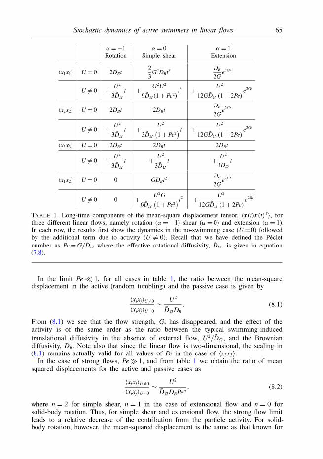
TABLE 1. Long-time components of the mean-square displacement tensor, 〈x(t)x(t)T〉, forthree different linear flows, namely rotation (α=−1) shear (α= 0) and extension (α= 1).In each row, the results first show the dynamics in the no-swimming case (U= 0) followedby the additional term due to activity (U 6= 0). Recall that we have defined the Pécletnumber as Pe=G/DΩ where the effective rotational diffusivity, DΩ , is given in equation(7.8).

In the limit Pe 1, for all cases in table 1, the ratio between the mean-squaredisplacement in the active (random tumbling) and the passive case is given by

〈xixj〉U 6=0

〈xixj〉U=0∼ U2

DΩDB. (8.1)

From (8.1) we see that the flow strength, G, has disappeared, and the effect of theactivity is of the same order as the ratio between the typical swimming-inducedtranslational diffusivity in the absence of external flow, U2/DΩ , and the Browniandiffusivity, DB. Note also that since the linear flow is two-dimensional, the scaling in(8.1) remains actually valid for all values of Pe in the case of 〈x3x3〉.

In the case of strong flows, Pe 1, and from table 1 we obtain the ratio of meansquared displacements for the active and passive cases as

〈xixj〉U 6=0

〈xixj〉U=0∼ U2

DΩDBPen, (8.2)

where n = 2 for simple shear, n = 1 in the case of extensional flow and n = 0 forsolid-body rotation. Thus, for simple shear and extensional flow, the strong flow limitleads to a relative decrease of the contribution from the particle activity. For solid-body rotation, however, the mean-squared displacement is the same as that known for


a swimmer in a quiescent fluid medium. This can be seen from a reference framewhich is rotating with the flow wherein the only orientation decorrelation mechanismfor an active particle is rotary diffusion and potentially tumbling (see below for afurther discussion).

8.2. Physical scalingsOne may use simple physical arguments to recover the scalings seen in table 1. Thearguments presented below are for particles without tumbling, and the generalizationto include run-and-tumble dynamics, as indicated above, may be done by way of aneffective rotary diffusivity.

We begin by recalling that, in a quiescent fluid, the characteristic step size scalesas U/DΩ , the decorrelation time scales as 1/DΩ , leading to a translational diffusivityscaling as U2/DΩ , and thus 〈x2〉 ∼ (U2/DΩ)t. This may now be used to obtain theconvectively enhanced scalings for the mean-square displacements in simple shearand extensional flow. For pure shear and in the weak flow limit, diffusion alongthe gradient direction leads to x2 ∼ [(U2/DΩ)t]1/2, and the corresponding distancetraversed along the flow direction is x1∼Gx2t, implying that 〈x1x1〉∼O((GU)2t3/DΩ).In the strong flow limit, the characteristic step size in the gradient direction isU/G, since the displacement due to swimming is cut off by the rotation due to theambient vorticity. The decorrelation time scales as 1/DΩ , leading to a flow-dependenttranslational diffusivity of (U/G)2DΩ and 〈x2x2〉 ∼ (U/G)2DΩ t. In turn, this impliesthat 〈x1x1〉 ∼ O((Gx2t)2) ∼ U2DΩ t3, which is the limiting form, for high Pe, of theresults for simple shear flow in table 1.

In the case of extensional flow, the deterministic terms imply that x1 ∼ eGt, andthus 〈x1x1〉 ∼ e2Gt − 1, for a swimmer starting from the origin. The prefactor in 〈x1x1〉,given by U2/(GDΩ), is obtained by Taylor expansion by noting that for times of orderD−1Ω (much smaller than G−1 in the weak flow limit), 〈x1x1〉 must still be diffusive.

In the strong flow limit, the prefactor scales as U2/G2, and is thus independent ofDΩ . In this limit, the decorrelation due to rotary diffusion occurs at a much largertime compared with the flow time scale, and there is thus a direct transition from theshort-time ballistic regime to the exponential enhancement driven by the ambient flow.

8.3. The peculiar case of solid-body rotationIt is of interest to note that diffusivity in solid-body rotation is unaffected by vorticitystrength, whereas in simple shear flow, the diffusivity in the gradient directiondecreases with flow strength as ∝G−2 as shown by the above scaling arguments. Theorbital frequency (time taken to complete an entire circuit along a closed streamline)and the rotation frequency (equal to half the ambient vorticity) are exactly the samefor an active particle in solid-body rotation, and this leads to the lack of dependenceon the flow vorticity. Solid-body rotation is thus a singular limit. For the familyof elliptic linear flows, with α = −|α|, that span the interval between simple shearand solid-body rotation, there is always a mismatch between the orbital frequency,G√|α|, and the rotation frequency, G(1 + |α|)/2. This mismatch leads to a finite

displacement in the deterministic limit. An active swimmer in an elliptic linear flowends up swimming indefinitely, and with a periodic reversal in direction, within aregion whose spatial extent is ∼U/[G(1−√|α|)]. The reversal in direction happenson a time scale of order G(1−√|α|)−1, and thus, the behaviour of the mean squaredisplacement in an elliptic linear flow depends on the relative magnitudes of theintrinsic decorrelation time, D−1

Ω , and the aforementioned deterministic reversal time.When D−1

Ω G(1 − √|α|)−1, then the long-time diffusivities along the principal


axes of the elliptical streamlines are independent of the flow strength; note that thisis the only limit relevant to solid-body rotation. In the strong flow limit, however,we have D−1

Ω G(1 − √|α|)−1, and the diffusivities scale as ∝ G−2. This, and theadditional dependence on |α|, may be obtained by noting that the characteristic stepsize is now of order U/[G(1−√|α|)], while the decorrelation time is still ∼D−1

Ω . So,the long-time diffusivity (along the minor axis of the closed streamlines) scales as(U/G(1−√|α|)2DΩ . The breakdown of this argument, and the flow-independence ofthe diffusivity for solid-body rotation, arises from the divergence of the elementarystep size in the limit α→−1.

8.4. Time scales for enhancementAnother issue of interest, in the case of shear flows, is the time one has to waitin order to observe the enhanced mean-square displacement, ∼t3, along the flowdirection, 〈x1x1〉. That time scale can be obtained by comparing the order ofmagnitudes of the ∼t2 and ∼t3 terms in (6.6). For a weak shear flow, Pe 1,we get a cross-over at a critical time scale such that DΩ t ∼ U2/(DΩDB + U2).Assuming that activity leads to enhanced mean-square displacement, we thus haveU2 DΩDB (see (8.1)), and therefore see that the cross-over occurs of the order ofthe rotational time scale, t ∼ D−1

Ω . In the case of a strong shear flow, Pe 1, weget that the cross over occurs when t ∼ U2/(U2DΩ + G2DB). If we assume again tobe in the enhanced regime, corresponding to U2 DΩDBG2τ 2 (see (8.2)), and thusU2DΩ G2DB, leading again to t ∼ D−1

Ω . The relevant time to obtain the enhancedmean square displacement is therefore independent on weak versus strong nature ofthe flow, and is always the typical orientation decorrelation time. A similar analysiscan be carried out for the cross-term, 〈x1x2〉, with similar results.

8.5. Relevance to biology and bioengineeringFrom a practical standpoint, when can we expect these results to be quantitativelyimportant? Let us consider a small biological or synthetic swimmer with a typicalsize of 1 µm. At room temperature and in water this leads to a Brownian diffusionconstant of DB ≈ 0.22 µm2 s−1 and DΩ ≈ 0.16 s−1 leading to a thermal time scaleof ≈3 s. The estimate in (8.1) says that, for weak flows, the critical swimmingspeed to observe an enhancement is Uc∼ (DΩDB)

1/2≈ 200 nm s−1. Micrometre-sizedswimmers, both biological (Lauga & Powers 2009) and synthetic (Mallouk & Sen2009), typically go much faster than this value, and thus the effect quantified hereshould result in enhancement by orders of magnitude and should be easily seenexperimentally.

In the presence of a strong flow, the critical swimming speed necessary in order toobserve an enhanced mean-square motion is increased due to the Pen term in equation(8.2). What is the typical value of a deformation rate, G, in a practical situation? Weconsider two cases. The first is that of planktonic bacteria (Guasto et al. 2012), whichare subject to wind-driven flows with root-mean-square (r.m.s.) deformation rates ofup to G∼ 10 s−1 on the smallest length scales (Jimenez 1997). These flows typicallypossess both extensional (n = 1) and viscous (n = 2) components and are typicallyturbulent, but given that the Kolmogorov length scale is at least a few millimetres, theyappear laminar on the scale of a micrometre-size organism. In that case, the criticalvelocity becomes Uc ∼ (DΩDB)

1/2(Pe)n/2 ∼ 1 µm s−1 for extensional flow and Uc ∼5 µm s−1 for shear and rotation. These swimming speeds are below typical velocitiesin biological locomotion, and thus the random motion of bacteria in oceanic flow isexpected to be strongly affected by their activity.


A second situation of interest would be that of synthetic swimmers in blood flow,where in this case the motion is dominated by shear (n= 2). In large blood vessels wehave G∼ 102 s−1 (Pedley 1980), leading to a critical swimming speed for enhancedmotion in a shear flow of Uc ∼ 50 µm s−1, on the upper limit of the syntheticswimming speeds measured in the laboratory. In contrast, for flow in capillarieswe have much larger deformation rates, up to G ∼ 104 s−1 (Lipowsky, Kovalcheck& Zweifach 1978), leading to a large value Uc ∼ 5 mm s−1. Whereas the randommotion of small synthetic swimmers is expected to be affected by both blood flowand the swimmer motion in large vessels, the effect of swimming in small capillarieswill probably be negligible.

8.6. Summary and perspectiveIn summary we have addressed theoretically the stochastic dynamics of sphericalactive particles diffusing in an incompressible, two-dimensional linear flow. Afterderiving the general framework valid for an arbitrary time-dependent swimmingvelocity of the particles, we focused on the special case of steadily swimmingparticles and have illustrated our analytical results on three different flows: solid-bodyrotation, simple shear and extension. We have also shown that the results can beextended to a particle which executes a run-and-tumble motion, as a model for thedynamics of bacteria. Compared with passive colloidal particles, we have shown thatthe activity of the particle leads to the same long-time scalings but with increasedvalues of the coefficients, which can be physically rationalized (see the summary intable 1). By comparing the new terms with those obtained for passive particles wehave shown that the activity of the particles could lead to enhancement by ordersof magnitude of their mean-square displacement, for example for planktonic bacteriasubject to oceanic turbulence. Our results could thus be further exploited to quantifythe ability of specific small-scale biological organisms to sample their surroundings.

The calculations in the paper were made under a number of assumptions whichsuggest ways in which the study could be generalized. We have assumed the flowsto be of an infinite extent, whereas for example in a biological setting it is clear thatthe presence of boundaries would play an important role. We have also assumed theactive particle to be spherical, allowing us to perform all calculations analytically. Fornon-spherical bodies, relevant for example for elongated bacteria, equation (2.1) wouldinclude an additional term which depends on the symmetric part of the rate-of-straintensor, and would require the use of numerical computations to derive the effectivelong-time dynamics of the active particle (or restriction of the analysis to certainasymptotic regimes in the rotary Péclet number). One important difference between thedynamics of spherical and non-spherical particles is that whereas spherical particlesundergo uniform rotation at a rate proportional to the flow vorticity, non-sphericalparticles rotate along Jeffery orbits, and for large aspect ratios, end up spending asignificant amount of time aligned in certain directions (the flow-vorticity plane insimple shear).

Finally, beyond thermal forces and run-and-tumble, other sources of directionalchange could be address with our modelling approach, in particular run-and-reversefor bacteria (Guasto et al. 2012), phase slips in eukaryotic flagella (Polin et al. 2009),collisions (Ishikawa & Pedley 2007) or even non-thermal turbulent fluctuations inflow vorticity in environmental flows (Jimenez 1997). Despite these limitations, wehope that our study will provide new insight into the interplay among orientationdecorrelation, external flows and activity, and will be valuable in order to developcoarse-grained theories of swimming populations in complex, external flows.


AcknowledgementsThis work was funded in part by the Consejo Nacional de Ciencia y Tecnologia

of Mexico (Conacyt postdoctoral fellowship to M. S.) and the US National ScienceFoundation (Grant CBET-0746285 to E.L.).

REFERENCES

ABBOTT, J. J., PEYER, K. E., LAGOMARSINO, M. C., ZHANG, L., DONG, L., KALIAKATSOS, I.K. & NELSON, B. J. 2009 How should microrobots swim?. Int. J. Robot. Res. 28, 1434–1447.

ABRAMOWITZ, M. & STEGUN, I. 1970 Handbook of Mathematical Functions. Dover.BEARON, R. N. & PEDLEY, T. J. 2000 Modelling run-and-tumble chemotaxis in a shear flow. Bull.

Math. Biol. 62, 775–791.BERG, H. C. 1993 Random walks in biology. Princeton University Press.BERG, H. C. 2004 E. coli in Motion. Springer.BERNE, B. J. & PECORA, R. 2000 Dynamic Light Scattering: with Applications to Chemistry, Biology,

and Physics. Dover.BRADY, J. F. 2010 Particle motion driven by solute gradients with application to autonomous motion:

continuum and colloidal perspectives. J. Fluid Mech. 667, 216–259.BRENNER, H. 1974 Rheology of a dilute suspension of axisymmetric Brownian particles. Intl J.

Multiphase Flow 1 (2), 195–341.BRENNER, H. & CONDIFF, D. W. 1974 Transport mechanics in systems of orientable particles. IV.

Convective transport. J. Colloid Interface Sci. 47 (1), 199–264.CLERCX, H. J. H. & SCHRAM, P. P. J. M. 1992 Brownian particles in shear fiow and harmonic

potentials: a study of long-time tails. Phys. Rev. A 46, 1942–1950.COFFEY, W., KALMIKOV, Y. P. & VALDRON, Y. T. 1996 The Langevin Equation: With Applications

in Physics, Chemistry and Electrical Engineering. World Scientific.DOI, M. & EDWARDS, S. F. 1999 The Theory of Polymer Dynamics. Clarendon Press.DRESCHER, K., LEPTOS, K. C., TUVAL, I., ISHIKAWA, T., PEDLEY, T. J. & GOLDSTEIN, R. E.

2009 Dancing volvox: hydrodynamic bound states of swimming algae. Phys. Rev. Lett. 102,168101.

FOISTER, R. T. & VAN DE VEN, T. G. M. 1980 Diffusion of Brownian particles in shear flows.J. Fluid Mech. 96, 105–132.

FRANKEL, I. & BRENNER, H. 1991 Generalized Taylor dispersion phenomena in unboundedhomogeneous shear flows. J. Fluid Mech. 230, 147–181.

FRANKEL, I. & BRENNER, H. 1993 Taylor dispersion of orientable Brownian particles in unboundedhomogeneous shear flows. J. Fluid Mech. 255, 129–156.

GOLESTANIAN, R., LIVERPOOL, T. B. & AJDARI, A. 2007 Designing phoretic micro- and nano-swimmers. New J. Phys. 9, 126.

GUASTO, J. S., RUSCONI, R. & STOCKER, R. 2012 Fluid mechanics of planktonic microorganisms.Annu. Rev. Fluid Mech. 44, 373–400.

HAUGE, E. H. & MARTIN-LÖF, A. 1973 Fluctuating hydrodynamics and Brownian motion.J. Stat. Phys. 7 (3), 259–281.

HINCH, E. J. 1975 Application of the Langevin equation to fluid suspensions. J. Fluid Mech. 72,499–511.

HOWSE, J. R., JONES, R. A. L., RYAN, A. J., GOUGH, T., VAFABAKHSH, R. & GOLESTANIAN,R. 2007 Self-motile colloidal particles: from directed propulsion to random walk. Phys. Rev.Lett. 99 (4), 048102.

ISHIKAWA, T. & PEDLEY, T. J. 2007 Diffusion of swimming model micro-organisms in a semi-dilutesuspension. J. Fluid Mech. 588, 437–462.

JIMENEZ, J. 1997 Oceanic turbulence at millimetre scales. Scientia Marina 61, 47–56.JONES, M. S., BARON, L. E. & PEDLEY, T. J. 1994 Biflagellate gyrotaxis in a shear flow.

J. Fluid Mech. 281, 137.JÜLICHER, F. & PROST, J. 2009 Generic theory of colloidal transport. Eur. Phys. J. E 29 (1), 27–36.KOCH, D. L. & SUBRAMANIAN, G. 2011 Collective hydrodynamics of swimming microorganisms:

living fluids. Annu. Rev. Fluid Mech. 43, 230602.


KOSA, G., JAKAB, P., SZEKELY, G. & HATA, N. 2012 MRI driven magnetic microswimmers. Biomed.Microdevices 14, 165.

LAUGA, E. 2011 Enhanced diffusion by reciprocal swimming. Phys. Rev. Lett. 106, 178101.LAUGA, E. & GOLDSTEIN, R. E. 2012 Dance of the microswimmers. Phys. Today 65 (9), 30–35.LAUGA, E. & POWERS, T. R. 2009 The hydrodynamics of swimming microorganisms. Rep. Prog.

Phys. 72, 096601.LEAL, L. G. & HINCH, E. J. 1971 The effect of weak Brownian rotations on particles in shear

flow. J. Fluid Mech. 46, 685–703.LIPOWSKY, H. H., KOVALCHECK, S. & ZWEIFACH, B. W. 1978 The distribution of blood rheological

parameters in the microvasculature of cat mesentery. Circulat. Res. 43, 738–749.LOCSEI, J. T. & PEDLEY, T. J. 2009 Run and tumble chemotaxis in a shear flow: the effect of

temporal comparisons, persistence, rotational diffusion, and cell shape. Bull. Math. Biol. 71,1089–1116.

LOVELY, P. S. & DAHLQUIST, F. W. 1975 Statistical measures of bacterial motility and chemotaxis.J. Theor. Biol. 50, 477–496.

MALLOUK, T. E. & SEN, A. 2009 Powering nanorobots. Sci. Am. 300, 72–77.MIRKOVIC, T., ZACHARIA, N. S., SCHOLES, G. D. & OZIN, G. A. 2010 Fuel for thought: chemically

powered nanomotors out-swim nature’s flagellated bacteria. ACS Nano 4, 1782–1789.OTHMER, H. G. , DUNBAR, S. R. & ALT, W. 1988 Models of dispersal in biological systems.

J. Math. Biol. 26 (3), 263–298.PAHLAVAN, A. A. & SAINTILLAN, D. 2011 Instability regimes in flowing suspensions of swimming

micro-organisms. Phys. Fluids 23, 011901.PAXTON, W. F., SUNDARARAJAN, S., MALLOUK, T. E. & SEN, A. 2006 Chemical locomotion.

Angew. Chem. Intl Ed. Engl. 45, 5420–5429.PEDLEY, T. J. 1980 The Fluid Mechanics of Large Blood Vessels. Cambridge University Press.PEDLEY, T. J. & KESSLER, J. O. 1992 Hydrodynamic phenomena in suspensions of swimming

microorganisms. Annu. Rev. Fluid Mech. 24, 313–358.POLIN, M., TUVAL, I., DRESCHER, K., GOLLUB, J. P. & GOLDSTEIN, R. E. 2009 Chlamydomonas

swims with two gears in a eukaryotic version of run-and-tumble locomotion. Science 325,487–490.

RAFAI, S., JIBUTI, L. & PEYLA, P. 2010 Effective viscosity of microswimmer suspensions. Phys.Rev. Lett. 104, 098102.

SAINTILLAN, D. 2010a Extensional rheology of active suspensions. Phys. Rev. E 81, 056307.SAINTILLAN, D. 2010b The dilute rheology of swimming suspensions: a simple kinetic model. Exp.

Mech. 50, 1275–1281.SAN-MIGUEL, M. & SANCHO, J. M 1979 Brownian motion in shear flow. Physica 99A, 357–364.SCHMITT, M. & STARK, H. 2013 Swimming active droplet: a theoretical analysis. Eur. Phys. Lett.

101, 44008.SUBRAMANIAN, G. & BRADY, J. F. 2004 Multiple scales analysis of the Fokker–Planck equation

for simple shear flow. Phys. A: Stat. Mech. Appl. 334 (3–4), 343–384.SUBRAMANIAN, G. & KOCH, D. L 2009 Critical bacterial concentration for the onset of collective

swimming. J. Fluid Mech. 632, 359–400.TEN HAGEN, B., VAN TEEFFELEN, S. & LOWEN, H. 2009 Non-Gaussian behaviour of a self-propelled

particle on a substrate. Cond. Mat. Phys. 12, 725–738.TEN HAGEN, B., VAN TEEFFELEN, S. & LOWEN, H. 2011a Brownian motion of a self-propelled

particle. J. Phys.: Condens. Matter 23, 194119.TEN HAGEN, B., WITTKOWSKI, R. & LOWEN, H. 2011b Brownian dynamics of a self-propelled

particle in shear flow. Phys. Rev. E 84, 031105.THUTUPALLI, S., SEEMANN, R. & HERMINGHAUS, S. 2011 Swarming behaviour of simple model

squirmers. New J. Phys. 13, 073021.WANG, J. & GAO, W. 2012 Nano/microscale motors: biomedical opportunities and challenges. ACS

Nano 6, 5745.ZWANZIG, R & BIXON, M 1970 Hydrodynamic theory of the velocity correlation function. Phys.

Rev. A 2 (5), 2005.

Documents

J. Fluid Mech. (2014), . 742, doi:10.1017/jfm.2013.651 ... · J. Fluid Mech. (2014), ... Stochastic dynamics of active swimmers in linear ˛ows Mario Sandoval1,2,†, Navaneeth K