J. Fluid Mech. (2013), . 737, pp. doi:10.1017/jfm.2013.580 ...perso.ens-lyon.fr/laurent.chevillard/MyPageFiles/Jfm737.pdf · special case of an axisymmetric ellipsoid, the evolution

J. Fluid Mech. (2013), vol. 737, pp. 571–596. c© Cambridge University Press 2013 571doi:10.1017/jfm.2013.580

Orientation dynamics of small,triaxial–ellipsoidal particles in isotropic

turbulence

Laurent Chevillard1,† and Charles Meneveau2

1Laboratoire de Physique de l’Ecole Normale Superieure de Lyon, CNRS, Universite de Lyon, 46 alleed’Italie F-69007 Lyon, France

2Department of Mechanical Engineering and Center for Environmental and Applied Fluid Mechanics,The Johns Hopkins University, 3400 N. Charles Street, Baltimore, MD 21218, USA

(Received 22 May 2013; revised 19 September 2013; accepted 29 October 2013)

The orientation dynamics of small anisotropic tracer particles in turbulent flowsis studied using direct numerical simulation (DNS) and results are comparedwith Lagrangian stochastic models. Generalizing earlier analysis for axisymmetricellipsoidal particles (Parsa et al., Phys. Rev. Lett., vol. 109, 2012, 134501), wemeasure the orientation statistics and rotation rates of general, triaxial–ellipsoidaltracer particles using Lagrangian tracking in DNS of isotropic turbulence. Triaxialellipsoids that are very long in one direction, very thin in another and of intermediatesize in the third direction exhibit reduced rotation rates that are similar to those ofrods in the ellipsoid’s longest direction, while exhibiting increased rotation rates thatare similar to those of axisymmetric discs in the thinnest direction. DNS results differsignificantly from the case when the particle orientations are assumed to be statisticallyindependent from the velocity gradient tensor. They are also different from predictionsof a Gaussian process for the velocity gradient tensor, which does not provide realisticpreferred vorticity–strain-rate tensor alignments. DNS results are also compared with astochastic model for the velocity gradient tensor based on the recent fluid deformationapproximation (RFDA). Unlike the Gaussian model, the stochastic model accuratelypredicts the reduction in rotation rate in the longest direction of triaxial ellipsoidssince this direction aligns with the flow’s vorticity, with its rotation perpendicular tothe vorticity being reduced. For disc-like particles, or in directions perpendicular tothe longest direction in triaxial particles, the model predicts noticeably smaller rotationrates than those observed in DNS, a behaviour that can be understood based on theprobability of vorticity orientation with the most contracting strain-rate eigendirectionin the model.

Key words: turbulent flows

1. IntroductionThe fate of anisotropic particles in fluid flows is of considerable interest in the

context of various applications, such as micro-organism locomotion (Pedley & Kessler1992; Saintillan & Shelley 2007; Koch & Subramanian 2011), industrial manufacturing

† Email address for correspondence: [email protected]

mailto:[email protected]

572 L. Chevillard and C. Meneveau

processes such as paper-making (Lundell, Soderberg & Alfredsson 2011), and naturalphenomena such as ice crystal formation in clouds (Pinsky & Khain 1998). In many ofthese applications, the flow is highly turbulent and the rotational dynamics, alignmenttrends and correlations of anisotropic particles (such as fibres, discs or more generalshapes) with the flow field become of considerable interest. For small tracer particleswhose size is smaller than the Kolmogorov scale, the local flow around the particlecan be considered to be inertia-free and Stokes flow solutions can be used to relate therotational dynamics of the particles to the local velocity gradient tensor. This problemwas considered in the classic paper by Jeffery (1922), who solved the problem ofStokes flow around a general triaxial–ellipsoidal object. He then derived, for thespecial case of an axisymmetric ellipsoid, the evolution equation for the orientationvector as function of the local velocity gradient tensor. Such dynamics lead tofascinating phenomena such as a rotation of rods when placed in a constant shear(Couette) flow and periodic motions on closed (Jeffery’s) orbits. The effects of suchmotions on the rheology of suspensions has been studied extensively, see e.g. Larson(1999).

In turbulent flows the velocity gradient tensor Aij = ∂ui/∂xj fluctuates and isdominated by small-scale motions, of the order of the Kolmogorov scale ηK , andmuch work has focused on rod-like particles whose size is smaller than ηK . Studiesof the orientation dynamics of such particles in turbulent flows have included thoseof Shin & Koch (2005) and Pumir & Wilkinson (2011) using isotropic turbulencedata from direct numerical simulation (DNS), those of Zhang et al. (2001) andMortensen et al. (2008) for particles in channel flow turbulence also using DNS, andthose of Bernstein & Shapiro (1994) and Newsom & Bruce (1998) using data fromlaboratory and atmospheric measurements, respectively. (We remark that Shin & Koch(2005) also consider fibres that are longer than ηK). In numerical studies, Lagrangiantracking is most often used to determine the particle trajectories and simultaneoustime integration of the Jeffery equation along the trajectory leads to predictions of theparticles’ orientation dynamics.

Generic properties of the orientation dynamics, such as the variance of thefluctuating orientation vector or its alignment trends may also be studied by makingcertain assumptions about the Lagrangian evolution of the carrier fluid’s velocitygradient, in particular about its symmetric and antisymmetric parts, the strain-ratetensor S = (A + A>)/2 and rotation-rate tensor Ω = (A − A>)/2. A number of recenttheoretical studies have been based on the assumption that these flow variables obeyisotropic Gaussian statistics, e.g. are the result of linear Ornstein–Uhlenbeck processes(see e.g. Brunk, Koch & Lion 1998; Pumir & Wilkinson 2011; Wilkinson & Kennard2012; Vincenzi 2013). This assumption facilitates a number of theoretical results thatmay be used to gain insights into some features of the orientational dynamics, such asin the limiting case of strong vorticity with a weak random straining background, inwhich analytical solutions for the full probability density are possible (Vincenzi 2013).In these studies, the crucial role of alignments between the particles and the vorticityhas been highlighted. As will be shown in the following, the relative alignment of thevorticity with the strain rate eigendirections, as first observed in Ashurst et al. (1987)is also crucially important.

In a recent study based on DNS of isotropic turbulence, Parsa et al. (2012) analysethe orientational dynamics of axisymmetric ellipsoids of any aspect ratio, that is,from rod-like shapes to spherical and disc-like shapes. They consider axisymmetricellipsoids with major semi-axes of length d1, d2, d3, with d2 = d3. The unit orientationvector p is taken to point in the direction of the axis of size d1. The parameter

Orientation dynamics of ellipsoids in turbulence 573

α = d1/d2 = d1/d3 describes uniquely the type of anisotropy: for α→∞ one has rodor fibre-like particles with p aligned with the axis, while for α→ 0 one has discs withp aligned perpendicular to the plane of the disc. For α→ 1, one has spheres for whichthe choice of p is arbitrary relative to the object’s geometry. Parsa et al. (2012) reportthe variance and flatness factors of the orientation vector’s rate of variation p in timealong fluid tracer trajectories. Strong dependencies of the variance as a function of αare observed. The trends differ significantly from results obtained when one assumesthat p and A are uncorrelated, or that A follows Gaussian statistics with no preferredvorticity–strain-rate alignments.

Both Shin & Koch (2005) and Parsa et al. (2012) observe that the non-trivialdependencies of the particle rotation variance as a function of α are associatedwith the alignment trends between flow vorticity and strain-rate eigenvectors. Theyremark that the orientation dynamics of anisotropic particles can thus serve as auseful diagnostic to examine the accuracy of Lagrangian models for the velocitygradient tensor in turbulence. Several Lagrangian stochastic models for the velocitygradient tensor in turbulence have been proposed in the literature (Girimaji & Pope1990a; Cantwell 1992; Jeong & Girimaji 2003; Chertkov, Pumir & Shraiman 1999;Chevillard & Meneveau 2006; Naso, Pumir & Chertkov 2007; Biferale et al. 2007). Asreviewed by Meneveau (2011), some of these models are for coarse-grained velocitygradients (Biferale et al. 2007) or tetrads of fluid particles (Chertkov et al. 1999;Naso et al. 2007), while others describe transient or quasi-steady state behaviour only(Cantwell 1992; Jeong & Girimaji 2003). To the best of the authors’ knowledge, onlytwo stochastic processes for the full velocity gradient tensor that includes realisticstrain–vorticity correlations lead to stationary statistics. The first is due to Girimaji &Pope (1990a). It enforces by construction that the pseudo-dissipation is a lognormalprocess, and several additional free parameters must be prescribed. The secondprocess is the recent fluid deformation approximation (RFDA) approach (Chevillard& Meneveau 2006) in which a physically motivated closure is used to model pressureHessian and viscous effects. Recent interest has also focused on the fate of particleslarger than ηK (see e.g. Zimmermann et al. 2011).

Here we shall focus on the case of inertia-free particles smaller than ηK , but ofa general ellipsoidal shape that is not necessarily axisymmetric. The aims of thepresent work are twofold. First, to generalize the results of Parsa et al. (2012)to the case of generalized ellipsoidal particles, not restricted to the special case ofbodies of revolution. For this purpose, we use a generalization of Jeffery’s equationwritten in a convenient form by Junk & Illner (2007) that can be considered asa reformulation of earlier developments for triaxial–ellipsoidal particles by Jeffery(1922), Bretherton (1962), Gierszewski & Chaffey (1978), Hinch & Leal (1979) andYarin, Gottlieb & Roisman (1997). The model, summarized in § 2, describes thedynamics of all three orientation vectors pointing in each of the ellipsoid’s majoraxes. The results depend upon two geometric parameters d1/d2 and d1/d3 that areequal for the axisymmetric cases. We aim to measure the variance and flatness of therates of change of the three orientation vectors as a function of these two parameters.Also, geometric features such as the alignments between these orientation vectorsand special local flow directions (vorticity and strain-rate eigendirections) will bereported. The results from analysis of DNS are presented in § 3. The observed relativealignments highlight the importance of correlations among vorticity and strain-rateeigendirections in determining the particle orientation dynamics.

A second goal of this study, presented in § 4, is to study the predictions of severalmodels. As also done by Parsa et al. (2012) for axisymmetric particles, we first


consider predictions of the variance of particle rotation assuming the particle alignmentis uncorrelated from the velocity gradient tensor. We also consider a Gaussian modelof the velocity gradient tensor in which vorticity–strain-rate alignments are absent.Then we consider a stochastic model for the velocity gradient tensor (Chevillard &Meneveau 2006, 2007) in which pressure and viscous effects are modelled based onthe RFDA. This model has been shown to yield realistic predictions of stationarystatistics for the velocity gradient in turbulence at moderate Reynolds numbers(Chevillard et al. 2008). While the model has been generalized to passive scalars(Gonzalez 2009), rotating turbulence (Li 2011) and magnetohydrodynamic (MHD)turbulence (Hater, Homann & Grauer 2011), the fate of general triaxial–ellipsoidalanisotropic particles acted upon by a velocity gradient tensor that evolves accordingto the RFDA model has not yet been examined. The model results are compared withthose from DNS and conclusions are presented in § 5.

2. Evolution equations for anisotropic particle orientationMany numerical and theoretical studies use the Jeffery equation (Jeffery 1922) to

predict the time evolution of the orientation of an axisymmetric ellipsoidal particle, asit is advected and acted on by a turbulent velocity field. Specifically, Jeffery’s equationfor the unit orientation vector p(t) in the ellipsoid major axis of size d1 (while d2 = d3

and α = d1/d2) reads

dpn

dt=Ωnjpj + λ(Snjpj − pnpkSklpl), (2.1)

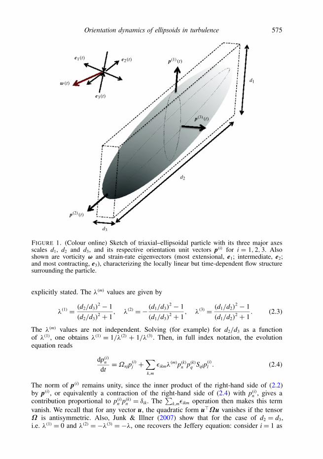
where λ = (α2 − 1)/(α2 + 1) and S and Ω are the strain- and rotation-rate tensors,respectively. This equation is valid for axisymmetric ellipsoids in which two semi-axes are equal. The case of more general geometries was considered by Bretherton(1962) in which the linearity of Stokes flow and general symmetries gave the generalform that any orientation evolution must have. Additional references dealing withthe orientation dynamics of general ellipsoids include Gierszewski & Chaffey (1978),Hinch & Leal (1979) and Yarin et al. (1997). For instance, Hinch & Leal (1979)found that slight deviations from axisymmetry may cause significant variations in theresulting rates of particle rotation. In a recent paper (Junk & Illner 2007), the resultswere cast in a practically useful form, namely a system of three equations describingthe evolution of three perpendicular unit vectors, each directed in one of the principaldirections of the ellipsoid. Figure 1 illustrates the geometry of a general triaxialellipsoid, exposed to the action of a surrounding local vorticity and strain-rate field atmuch larger scales. Since Stokes flow is assumed, the result is applicable only whenthe size of the tracer particle, i.e. its largest dimension, is smaller than the Kolmogorovscale of turbulence.

The Junk & Illner equation reads, for the three perpendicular unit vectors p(i)

(i= 1, 2, 3):

dp(i)

dt= 1

2(∇ × u)× p(i) +

∑k,m

εikmλ(m)p(k) ⊗ p(k)Sp(i), (2.2)

where ⊗ stands for the tensorial product, i.e. for any vectors u and v, we have(u⊗ v)ij = uivj. Moreover, we sum over repeated subscript indices (i.e. Einsteinconvention), but we do not sum over repeated superscripts in parenthesis, unless


FIGURE 1. (Colour online) Sketch of triaxial–ellipsoidal particle with its three major axesscales d1, d2 and d3, and its respective orientation unit vectors p(i) for i = 1, 2, 3. Alsoshown are vorticity ω and strain-rate eigenvectors (most extensional, e1; intermediate, e2;and most contracting, e3), characterizing the locally linear but time-dependent flow structuresurrounding the particle.

explicitly stated. The λ(m) values are given by

λ(1) = (d2/d3)2 − 1

(d2/d3)2 + 1

, λ(2) =− (d1/d3)2 − 1

(d1/d3)2 + 1

, λ(3) = (d1/d2)2 − 1

(d1/d2)2 + 1

. (2.3)

The λ(m) values are not independent. Solving (for example) for d2/d3 as a functionof λ(1), one obtains λ(1) = 1/λ(2) + 1/λ(3). Then, in full index notation, the evolutionequation reads

dp(i)n

dt=Ωnjp

(i)j +

∑k,m

εikmλ(m)p(k)n p(k)q Sqlp

(i)l . (2.4)

The norm of p(i) remains unity, since the inner product of the right-hand side of (2.2)by p(i), or equivalently a contraction of the right-hand side of (2.4) with p(i)n , gives acontribution proportional to p(i)n p(k)n = δik. The

∑k,mεikm operation then makes this term

vanish. We recall that for any vector u, the quadratic form u>Ωu vanishes if the tensorΩ is antisymmetric. Also, Junk & Illner (2007) show that for the case of d2 = d3,i.e. λ(1) = 0 and λ(2) =−λ(3) =−λ, one recovers the Jeffery equation: consider i= 1 as


the main axis. Then we have∑k,m

ε1kmλ(m)p(k) ⊗ p(k)Sp(i) =−λ(2)p(3) ⊗ p(3)Sp(1) + λ(3)p(2) ⊗ p(2)S p(1)

= λ (p(3) ⊗ p(3) + p(2) ⊗ p(2))

Sp(1). (2.5)

Since the three unit vectors form an orthogonal basis, we can use the fact that

p(1) ⊗ p(1) + p(2) ⊗ p(2) + p(3) ⊗ p(3) = I (2.6)

to obtain ∑k,m

ε1kmλ(m)p(k) ⊗ p(k)Sp(i) = λ (I − p(1) ⊗ p(1)

)Sp(1), (2.7)

which is the last term in the Jeffery equation (equation (2.1)) taking p(1) = p.Under the assumption of small inertia-free particles, the ellipsoid’s centroid follows

the fluid flow. Therefore, the time evolution in (2.2) can be interpreted as the evolutionalong fluid particle trajectories and the time evolution of the orientations dependssolely on the velocity gradient tensor. Knowing Ωij(t) and Sij(t) along fluid trajectoriesthus allows us to evaluate the Lagrangian evolution of particle orientations p(i) bysolving (2.2) (one may of course only solve for two components, since at all times,e.g. p(3) = p(1) × p(2)).

In this article, we are interested in the variance of the rate of rotation of theseorientation vectors (tumbling rates), extending the results for the variance of p(1) whend2 = d3 and d1/d2→+∞ (i.e. rods) studied by Shin & Koch (2005), and those ofParsa et al. (2012) for any d1/d2 with d2 = d3 (i.e. from rods to discs). Specifically, weare interested in the variance of the rotation speed of each direction vector as functionof the two independent anisotropy parameters,

V (i)

(d1

d2,

d1

d3

)= 1

2〈ΩrsΩrs〉〈p(i)n p(i)n 〉 (2.8)

for the three orientation vectors i = 1, 2, 3, and we recall that no summation isassumed over superscripts (i). In (2.8), the average of the square norm |p(i)|2 isnormalized by the average rate-of-rotation of the flow. We recall that for isotropicturbulence, 2〈ΩrsΩrs〉 = 2〈SrsSrs〉 = ε/ν, where ε is the average dissipation per massand ν the kinematic viscosity. Following Parsa et al. (2012) we are also interested inthe flatness factor, namely

F(i)

(d1

d2,

d1

d3

)= 〈(p

(i)n p(i)n )

2〉〈p(i)r p(i)r 〉2

. (2.9)

Further extending the prior analyses, we are also interested in the alignments betweenp(i) and the vorticity and strain-rate eigenvectors in the flow.

3. Orientation dynamics of triaxial ellipsoids in DNS of isotropic turbulenceIn this section, we consider orientation dynamics of triaxial ellipsoids in isotropic

turbulence at moderate Reynolds number. We use results from DNS of forcedisotropic turbulence at Rλ ≈ 125 to provide Lagrangian time histories of the velocitygradient tensor Aij(t) along the tracer particle trajectories. These data are the sameas those used by Chevillard & Meneveau (2011). The DNS is based on a pseudo-spectral method, de-aliased according to the 3/2 rule and with second-order accurate


Adams–Bashforth time stepping. The computational box is cubic (size 2π) withperiodic boundary conditions in the three directions and a spatial mesh with 2563

grid points. Statistical stationarity is maintained by an isotropic external force actingat low wavenumbers in order to ensure a constant power injection. It provides,in the units of the simulation, a constant energy injection rate of ε = 0.001. Thekinematic viscosity of the fluid is ν = 0.0004. The Kolmogorov scale is ηK = 0.016so that 1x/ηK ≈ 1.5 (with 1x = 2π/256). Lagrangian trajectories are obtained usingnumerical integration of the fluid tracer equation. A second-order time integrationscheme is used (involving both velocity and acceleration at the current spatiallocation), with a time step 1t = 3.5 × 10−3 and cubic spatial interpolation in thethree spatial directions to obtain velocity and acceleration at particle locations. A totalof 512 such trajectories, of length of order of 15 large-eddy turnover times, is usedin this study, with initial positions chosen at random in the flow volume. We havetested for statistical convergence levels using fewer and shorter trajectories (data notshown) and obtained results with negligible deviations from those plotted. Statisticalquantities shown, including the flatness, have converged statistically to levels equalto or smaller than the amplitudes of the deviations from smooth behaviour shownin the plots (i.e. better than ∼3 %). Once we have the Lagrangian time history ofthe velocity gradient tensor A(t), we integrate numerically the dynamics of the threevectors p(i) starting from three unit vectors that point in arbitrary (randomly chosen)initial directions, constrained by the orthonormality condition pq

(i)(0) = δiq. For highaccuracy (e.g. always checking that the set of three vectors remains orthonormal), weintegrate (2.2) using a standard fourth-order Runge–Kutta method, using the same timestep as used in the time integration to obtain the time history of A(t).

3.1. Variance and flatness of the time derivative of orientation vectors

We focus in this section on the variance V (i)(d1/d2, d1/d3) of the orientation vectors asdefined in (2.8). The sketch in figure 2 represents the various limiting geometries andorientation vectors as function of the ratios d1/d2 and d1/d3. Owing to the symmetriesinherent in the labelling of the various directions, interchanging d2 and d3 whileleaving d1 unchanged should not affect the rotation rates in the i= 1 direction. Hence,the results are expected to be symmetric around the 45 line (d1/d2 = d1/d3), i.e.

V (1)

(d1

d2,

d1

d3

)= V (1)

(d1

d3,

d1

d2

). (3.1)

Also, since upon interchanging the two directions (2) and (3), the correspondingdirection vector must be interchanged, we expect

V (3)

(d1

d3,

d1

d2

)= V (2)

(d1

d2,

d1

d3

), (3.2)

and hence only results for V (1) and V (2) are presented. The same symmetries apply tothe flatness factor, and hence only results for F(1) and F(2) are presented.

In figure 3 we show the normalized variance as function of the two ratios ofsemi-axes length, obtained from DNS. Several observations may be made based onthese results. First, for axisymmetric ellipsoids along the d1/d3 = d1/d2 line, the resultsfor V (1) agree with those of Parsa et al. (2012). Namely, for fibre-like ellipsoids(d1/d2→∞), the normalized variance tends to values near 0.09, whereas for disc-likeellipsoids, it tends to values near 0.24. For spherical particles, it is near 0.17. Thetrend at the edges of the negative 45 line, d1/d3 = (d1/d2)

−1 represent particles


2

2

1

1

0

0

–1

–1

–2

–2

FIGURE 2. Sketch of triaxial ellipsoid geometries and orientation vectors, as function ofsemi-axes ratios d1/d2 and d1/d3.

–1

0

1

–2 –1 0 1 2 –2 –1 0 1 2

0.10

0.12

0.14

0.16

0.18

0.20

0.22D

NS

–2

2

(a) (b)

FIGURE 3. (Colour online) Variance of rate-of-change of two ellipsoid orientation vectors p1

and p2 as function of the two ratios of semi-axes length, obtained from DNS. Contour lines gofrom 0.1 to 0.22 separated by 0.02: (a) V (1); (b) V (2).

that are long in one direction (e.g. d2 d1), very thin in another (d3 d1) andof intermediate size (d1) in the direction chosen for p(1). As can be seen, V (1)

along this line remains near the spherical value, with a small increase towardsV (1)(d1/d2→ 0, d1/d3→∞)∼ 0.19.


–1

0

1

–2 –1 0 1 2 –2 –1 0 1 2

6

7

8

9

DN

S

–2

2

(a) (b)

FIGURE 4. (Colour online) Flatness of rate-of-change of two ellipsoid orientation vectors p(1)and p(2) as function of the two ratios of semi-axes length, obtained from DNS. Contour linescorrespond to flatness values of 2.1, 2.2, 3, 3.8, 5, 6, 7, 8, 9: (a) F(1); (b) F(2).

The variance V (2) of the orientation vector in a direction perpendicular to p(1) andalong the direction of either the longest or shortest ellipsoid axis exhibits significantdependence upon the semi-axes scale ratios. For p(2) aligned along the largest ellipsoidsemi-axis (figure 3a), the variance is reduced, to about 0.09. This is similar to thevariance for long axisymmetric fibres. For p(2) aligned along the shortest ellipsoidsemi-axis (figure 3b), the variance is large, of the order of 0.24, similar to thevalues for axisymmetric discs. It was noted by Parsa et al. (2012) that the transitionbetween rod and disc-like behaviours occurred quite rapidly, with aspect ratios ofabout d1/d2 ∼ 2–3 already showing results quite close to the asymptotic values. As canbe seen in the results for V (2), the transition is even more rapid along the negative45, d1/d3 = (d1/d2)

−1 line, where most of the change in variance occurs for valuesbetween d1/d2 ∼ 0.6 and 1.6.

Next, the flatness factors of the orientation rates-of-change, F(1) and F(2) (equation(2.9)) are presented, in figure 4. As found by Parsa et al. (2012) for axisymmetriccases, the flatness is in a range between 5 and 10. These values are clearly above5/3, which is the value obtained when the vector p(1) is assumed to have zero-average independent Gaussian components (Parsa et al. 2012) or 2, which is the valueobtained for spheres (i.e. d1 = d2 = d3) when p(1) is assumed independent from velocitygradients, themselves assumed Gaussian (see Appendix and (A 15)). The maximumflatness is observed near the top middle and right middle regions, where d1 ≈ d2 andd3 d1 or d1 ≈ d3 and d1 ≈ d2, respectively, i.e. disc-like shapes, but with p(1) alignedin the plane of the disc. These were cases where the variance is relatively small (seefigure 3). For F(2), the structure is more complex, but the limiting cases showing peakflatness values are consistent with the results for F(1): namely the peaks occur fordisc-like shapes with the orientation vector aligned in the plane of the disc. Consistentwith the values of flatness that significantly exceed the Gaussian value and equivalentto the results of Parsa et al. (2012), the probability density functions (p.d.f.s) of p(i)n p(i)nshow elongated tails (data not shown).


0.5

1.0

1.5

2.0

2.5

3.0

3.5

–2 –1 0 1 2

0.5

DN

S

1.0

0

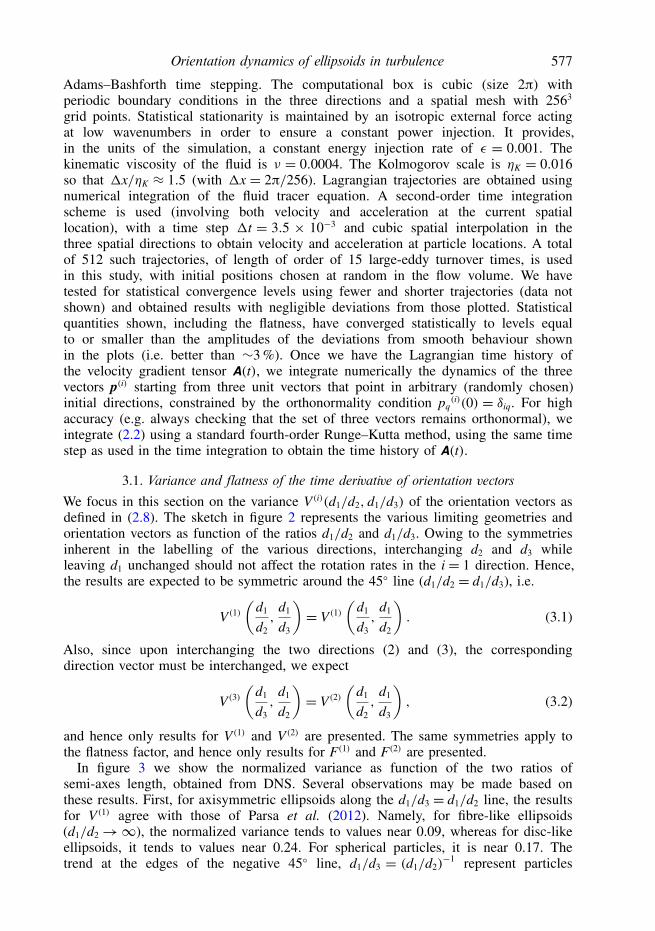
FIGURE 5. (Colour online) P.d.f. of the cosine of the angle between the vorticity direction ωand the ellipsoid’s major axis p(1) for axisymmetric case (i.e. d2 = d3), as a function of theanisotropy parameter d1/d2, obtained from DNS. Contour lines correspond to p.d.f. values of0.5, 1, 1.2, 1.5, 2.

3.2. Alignments of orientation vectors with vorticity and strain eigenframeNext, we consider the alignment trends of particle orientation with respect to thevorticity and strain-rate tensor’s eigendirections. For this discussion, we focus onthe case of axisymmetric particles and hence focus only on the single orientationvector p(1). Alignment trends with vorticity are quantified by measuring the p.d.f. ofcos(θp1ω) = p(1) · ω of the angle between p(1) and the vorticity direction ω = ω/|ω|.Results are shown in figure 5 as a function of the parameter α = d1/d2.

As can be seen, for fibre or rod-like particles (d1/d2 →∞), the results confirmstrong alignment with vorticity, a well-known trend found in many prior studies ofalignments of line elements in turbulence (Girimaji & Pope 1990b; Shin & Koch2005; Pumir & Wilkinson 2011). In the other limit, for disc-like particles, the resultsshow that p(1) is more preferentially perpendicular to the vorticity. That is to say, thevorticity tends to be in the plane of the disc. These orientation trends help understandthe parameter dependencies seen in the variance of p(1), i.e. V (1) shown in figure 3.Specifically, along the diagonal d1/d2 = d1/d3 for long rods (i.e. d1/d2 →∞), theparticle rotates along its axis of symmetry since p(1) is preferentially aligned with thevorticity. This leads to a reduced level of fluctuations V (1) (Shin & Koch 2005; Parsaet al. 2012). For discs, i.e. d1/d2 → 0, the vorticity is preferentially aligned in theplane of the disc which, like a spinning coin on a table, implies faster rotation of theorientation vector perpendicular to that plane.

A similar analysis is done for alignments with each of the strain-rate eigendirections.The alignments of p(1) with each of the strain-rate eigenvectors are quantified using thep.d.f. of the respective angle cosines. The results are shown in figure 6. The strongestalignment trend observed from the DNS is for disc-like particles to align with the mostcontracting eigendirection (figure 6c). This trend is quite easy to understand intuitively:the disc-plane tends to become perpendicular to the incoming (contracting) relative


0.5

–2 –1 0 1 2 –2 –1 0 1 2 –2 –1 0 1 2

0.5

1.0

1.5

DN

S

1.0

0

(a) (b) (c)

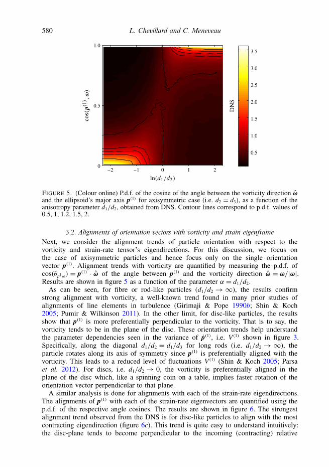
FIGURE 6. (Colour online) P.d.f. of cosine of angle between the strain-rate tensoreigendirections ei and the axisymmetric ellipsoid’s major axis p(1) for axisymmetric case,as function of the anisotropy parameter d1/d2 = d1/d3, obtained from DNS. Here e1 is thedirection of strongest extension (i.e. most positive eigenvalue), whereas e3 is the direction ofstrongest contraction (i.e. most negative eigenvalue). Contour lines correspond to p.d.f. valuesof 0.5, 0.8, 1, 1.2, 1.5: (a) p.d.f. cos(p(1), e1); (b) p.d.f. cos(p(1), e2); (c) p.d.f. cos(p(1), e3).

local flow direction. In addition, recall that the vorticity is perpendicular to the mostcontracting direction (data not shown, see Meneveau (2011)). The other trend that isvisible is that rod-like particles tend to become perpendicular to the most contractingdirection. This trend is consistent with its alignment with the vorticity, which tendsto be perpendicular to the most contractive direction. As observed previously, rod-likeparticles tend to align well with the intermediate eigenvectors, while disc-like particlesshow preponderance of perpendicular orientation with regards to the intermediateeigenvector. Interestingly, alignment with the most stretching eigendirection appearsto be very weak, almost random.

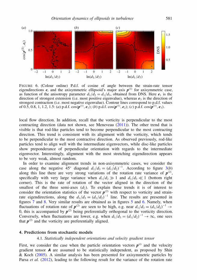
In order to examine alignment trends in non-axisymmetric cases, we consider thecase along the negative 45 diagonal d1/d3 = (d1/d2)

−1. According to figure 3(b)along this line there are very strong variations of the rotation rate variance of p(2),specifically with very large variance when d1/d2 1 and d1/d3 1 (bottom rightcorner). This is the rate of rotation of the vector aligned in the direction of thesmallest of the three semi-axes (d2). To explain these trends it is of interest toconsider the orientation statistics of the vector p(2) with respect to vorticity and strain-rate eigendirections, along the d1/d3 = (d1/d2)

−1 line. The results are presented infigures 7 and 8. Very similar results are obtained as in figures 5 and 6. Namely, whenfluctuations of rotation rate of p(2) are seen to be high, e.g. near d1/d3 = (d1/d2)

−1→0, this is accompanied by p(2) being preferentially orthogonal to the vorticity direction.Conversely, when fluctuations are lower, e.g. when d1/d3 = (d1/d2)

−1→∞, one seesthat p(2) and the vorticity are preferentially aligned.

4. Predictions from stochastic models4.1. Statistically independent orientations and velocity gradient tensor

First, we consider the case when the particle orientation vectors p(i) and the velocitygradient tensor A are assumed to be statistically independent, as proposed by Shin& Koch (2005). A similar analysis has been presented for axisymmetric particles byParsa et al. (2012), leading to the following result for the variance of the rotation rate


0.5

–2 –1 0 1 2

0.5

1.0

1.5

2.0

2.5

3.0

3.5

DN

S

1.0

0

FIGURE 7. (Colour online) P.d.f. of cosine of angle between the vorticity direction ω and theellipsoid’s second semi-axis p(2), as function of the anisotropy parameters d1/d3 = (d1/d2)

−1,obtained from DNS. Contour lines correspond to p.d.f. values of 0.5, 1, 1.2, 1.5, 2.

0.5

–2 –1 0 1 2 –2 –1 0 1 2 –2 –1 0 1 2

0.5

1.0

1.5

DN

S

1.0

0

(a) (b) (c)

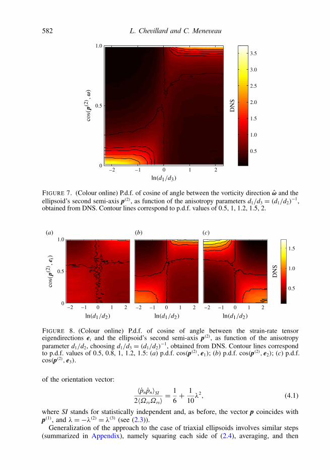
FIGURE 8. (Colour online) P.d.f. of cosine of angle between the strain-rate tensoreigendirections ei and the ellipsoid’s second semi-axis p(2), as function of the anisotropyparameter d1/d2, choosing d1/d3 = (d1/d2)

−1, obtained from DNS. Contour lines correspondto p.d.f. values of 0.5, 0.8, 1, 1.2, 1.5: (a) p.d.f. cos(p(2), e1); (b) p.d.f. cos(p(2), e2); (c) p.d.f.cos(p(2), e3).

of the orientation vector:

〈pnpn〉SI

2〈ΩrsΩrs〉 =16+ 1

10λ2, (4.1)

where SI stands for statistically independent and, as before, the vector p coincides withp(1), and λ=−λ(2) = λ(3) (see (2.3)).

Generalization of the approach to the case of triaxial ellipsoids involves similar steps(summarized in Appendix), namely squaring each side of (2.4), averaging, and then


Unc

orre

late

d

–2

–1

0

1

2

–2 –1 0 1 2 –2 –1 0 1 2

0.18

0.20

0.22

0.24

(a) (b)

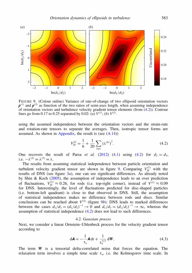
FIGURE 9. (Colour online) Variance of rate-of-change of two ellipsoid orientation vectorsp(1) and p(2) as function of the two ratios of semi-axes length, when assuming independenceof orientation vectors and turbulence velocity gradient tensor elements (from (4.2)). Contourlines go from 0.17 to 0.25 separated by 0.02: (a) V (1); (b) V (2).

using the assumed independence between the orientation vectors and the strain-rateand rotation-rate tensors to separate the averages. Then, isotropic tensor forms areassumed. As shown in Appendix, the result is (see (A 14))

V (i)SI =

16+ 1

20

∑k 6=i

(λ(k))2. (4.2)

One recovers the result of Parsa et al. (2012) (4.1) using (4.2) for d2 = d3,i.e. −λ(2) = λ(3) = λ.

The results from assuming statistical independence between particle orientation andturbulent velocity gradient tensor are shown in figure 9. Comparing V (1)

SI with theresults of DNS (see figure 3a), one can see significant differences. As already notedby Shin & Koch (2005), the assumption of independence leads to an over predictionof fluctuations, V (1)

SI ≈ 0.26, for rods (i.e. top-right corner), instead of V (1) ≈ 0.09for DNS. Interestingly, the level of fluctuations predicted for disc-shaped particles(i.e. bottom-left quadrant) is close to that observed in DNS. Still, the assumptionof statistical independence makes no difference between rods and discs. Similarconclusions can be reached about V (2) (figure 9b): DNS leads to marked differencesbetween the cases d1/d3 = (d1/d2)

−1 → 0 and d1/d3 = (d1/d2)−1 →∞, whereas the

assumption of statistical independence (4.2) does not lead to such differences.

4.2. Gaussian processNext, we consider a linear Ornstein–Uhlenbeck process for the velocity gradient tensoraccording to

dA=− 1τη

A dt + 1

τ3/2η

dW . (4.3)

The term W is a tensorial delta-correlated noise that forces the equation. Therelaxation term involves a simple time scale τη, i.e. the Kolmogorov time scale. In


this linear equation, the 1-point covariance structure of the velocity gradients A isimposed by the covariance structure of the tensorial forcing term dW , whereas thedamping term −A/τη enforces an exponential time correlation. To ensure isotropicstatistics for A, we use (see appendix A of Chevillard et al. (2008))

dWij(t)= DijpqdBpq(t), (4.4)

where B is a tensorial Wiener process with independent elements, i.e. its incrementsare Gaussian, independent and satisfy

〈dBpq〉 = 0 and 〈dBij(t)dBkl(t)〉 = 2 dtδikδjl, (4.5)

and the diffusion kernel is Dijpq chosen as

Dijpq = 13

3+√15√10+√6

δijδpq −√

10+√64

δipδjq + 1√10+√6

δiqδjp. (4.6)

For such a process, one obtains in the stationary regime

〈Aij(t)Akl(t + τ)〉 =t→∞

1τ 2η

e−|τ |/τη[

2δikδjl − 12δijδkl − 1

2δilδjk

], (4.7)

which is consistent with a covariance structure of a trace-free, homogeneous andisotropic tensor, exponentially correlated in time, and such that the variance ofdiagonal (respectively off-diagonal) elements is τ−2

η (respectively 2τ−2η ). Accordingly,

the covariance structure of its symmetric part is

〈Sij(t)Skl(t + τ)〉 =t→∞

14τ 2

η

e−|τ |/τη[3δikδjl − 2δijδkl + 3δilδjk

], (4.8)

and

〈Ωij(t)Ωkl(t + τ)〉 =t→∞

54τ 2

η

e−|τ |/τη[δikδjl − δilδjk

](4.9)

for the antisymmetric part. Remark that with this definition of τη, we get 〈2SpqSpq〉 =〈2ΩpqΩpq〉 = 〈ApqApq〉 = 15/τ 2

η = ε/ν.Simulation of this tensorial process generates a time series of A(t) which is used in

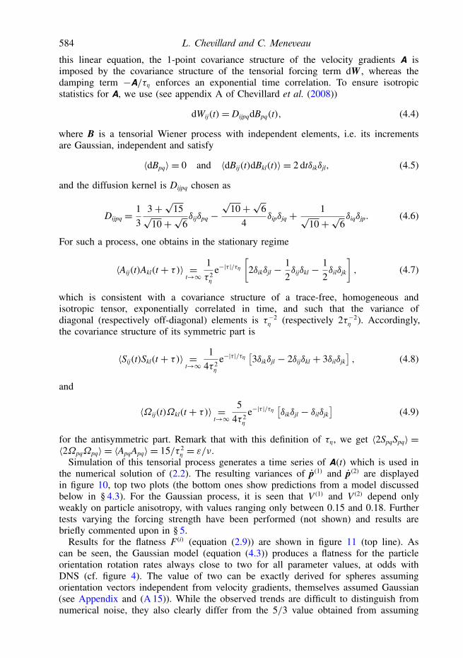
the numerical solution of (2.2). The resulting variances of p(1) and p(2) are displayedin figure 10, top two plots (the bottom ones show predictions from a model discussedbelow in § 4.3). For the Gaussian process, it is seen that V (1) and V (2) depend onlyweakly on particle anisotropy, with values ranging only between 0.15 and 0.18. Furthertests varying the forcing strength have been performed (not shown) and results arebriefly commented upon in § 5.

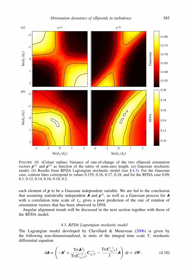
Results for the flatness F(i) (equation (2.9)) are shown in figure 11 (top line). Ascan be seen, the Gaussian model (equation (4.3)) produces a flatness for the particleorientation rotation rates always close to two for all parameter values, at odds withDNS (cf. figure 4). The value of two can be exactly derived for spheres assumingorientation vectors independent from velocity gradients, themselves assumed Gaussian(see Appendix and (A 15)). While the observed trends are difficult to distinguish fromnumerical noise, they also clearly differ from the 5/3 value obtained from assuming


RFD

A

Gau

ssia

n

–2

–1

0

1

2

–2

–1

0

1

2

–2 –1 0 1 2 –2 –1 0 1 2

0.155

0.160

0.165

0.170

0.175

0.180

0.10

0.12

0.14

0.16

0.18

0.20

(a)

(b)

FIGURE 10. (Colour online) Variance of rate-of-change of the two ellipsoid orientationvectors p(1) and p(2) as function of the ratios of semi-axes length. (a) Gaussian stochasticmodel. (b) Results from RFDA Lagrangian stochastic model (see § 4.3). For the Gaussiancase, contour lines correspond to values 0.155, 0.16, 0.17, 0.18, and for the RFDA case 0.09,0.1, 0.12, 0.14, 0.16, 0.18, 0.2.

each element of p to be a Gaussian independent variable. We are led to the conclusionthat assuming statistically independent A and p(i), as well as a Gaussian process for Awith a correlation time scale of τη, gives a poor prediction of the rate of rotation oforientation vectors that has been observed in DNS.

Angular alignment trends will be discussed in the next section together with those ofthe RFDA model.

4.3. RFDA Lagrangian stochastic modelThe Lagrangian model developed by Chevillard & Meneveau (2006) is given bythe following non-dimensionalized, in units of the integral time scale T , stochasticdifferential equation

dA=(−A2 + Tr(A2)

Tr(C−1τη/T)

C−1τη/T− Tr(C−1

τη/T)

3A

)dt + dW . (4.10)


RFD

A

Gau

ssia

n

–2

–1

0

1

2

–2

–1

0

1

2

–2 –1 0 1 2 –2 –1 0 1 2

2.1

2.2

2.3

2.4

2.5

3.0

3.5

(a)

(b)

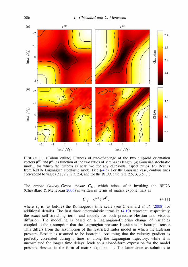
FIGURE 11. (Colour online) Flatness of rate-of-change of the two ellipsoid orientationvectors p(1) and p(2) as function of the two ratios of semi-axes length. (a) Gaussian stochasticmodel, for which the flatness is near two for any ellipsoidal aspect ratios. (b) Resultsfrom RFDA Lagrangian stochastic model (see § 4.3). For the Gaussian case, contour linescorrespond to values 2.1, 2.2, 2.3, 2.4, and for the RFDA case, 2.2, 2.5, 3, 3.5, 3.8.

The recent Cauchy–Green tensor Cτη , which arises after invoking the RFDA(Chevillard & Meneveau 2006) is written in terms of matrix exponentials as

Cτη = eτηAeτηA>, (4.11)

where τη is (as before) the Kolmogorov time scale (see Chevillard et al. (2008) foradditional details). The first three deterministic terms in (4.10) represent, respectively,the exact self-stretching term, and models for both pressure Hessian and viscousdiffusion. The modelling is based on a Lagrangian–Eulerian change of variablescoupled to the assumption that the Lagrangian pressure Hessian is an isotropic tensor.This differs from the assumption of the restricted Euler model in which the Eulerianpressure Hessian is assumed to be isotropic. Assuming that the velocity gradient isperfectly correlated during a time τK along the Lagrangian trajectory, while it isuncorrelated for longer time delays, leads to a closed-form expression for the modelpressure Hessian in the form of matrix exponentials. The latter arise as solutions to


the kinematic equation for the deformation tensor. A similar derivation can be done forthe Laplacian that arises in the viscous term. An analysis of expansions of the matrixexponentials is provided by Martins-Afonso & Meneveau (2010). The term W is thesame tensorial delta-correlated noise term that enters in the Gaussian process (equation(4.3)), it represents possible forcing effects, e.g. from neighbouring eddies.

The RFDA model has been shown to reproduce several important characteristics ofthe velocity gradient tensor, such as the preferential alignments of vorticity with theintermediate eigendirection of the strain and subtle temporal correlations (Chevillard &Meneveau 2011). It has thus a more complex covariance structure than that obtainedfrom the Ornstein–Uhlenbeck process (equation (4.3)) and is more realistic (seeChevillard et al. 2008; Meneveau 2011). Yet, the model has some known limitations:as discussed further by Meneveau (2011), extensions to increasing Reynolds number(reducing τη/T below 10−2 or so) leads to unphysical tails in the velocity gradientp.d.f.s. Also, tests have shown that the process leads to small deviations between thevariance of the strain-rate tensor and the rotation rate tensor, i.e. for τη/T = 0.1, weobtain 〈SijSij〉 ≈ 1.1〈ΩijΩij〉. Further strengths and limitations of the model will behighlighted by comparing its predictions of particle orientation dynamics to DNS.

The process is simulated numerically using a standard second-order Runge–Kuttaalgorithm with a unique realization of the noise for each time step. The time series ofA(t) generated by this process are, again, used in the solution of (2.2). The resultingvariances of p(1) and p(2) are displayed in the bottom row of plots in figure 10. As canbe seen, certain trends agree well with the results from the DNS. As opposed to theresults from the Gaussian model, in the limit of rod-like particles (d1/d2 = d1/d3 1),the variance of p(1) decreases significantly. Alignment of p(1) with the vorticity leads toa reduction of its rate of change. In the other limit (d1/d2 = d1/d3 1), however,the model predicts also some reduction of variance, unlike the DNS results. Tobetter understand the origin of this result, the alignments of p(1) with the strain-rateeigensystem will be quantified and compared with DNS.

In terms of the variance of p(2) shown in figure 10(d), we remark that there is goodoverall agreement between the model and DNS results: in the top left corner thereis decreased variance, while towards the bottom-right corner the variance is generallyhigher. Nevertheless, a non-monotonic behaviour is observed here too, in which somedecrease in variance towards d1/d2 1 can be observed.

In order to enable quantitative comparisons between DNS, the Gaussian model(equation (4.3)), and the RFDA model (equation (4.10)), we present sample resultsalong the d1/d2 = d1/d3 line of parameters, i.e. the axisymmetric cases. Figure 12shows the variance of p(1) for the DNS, Gaussian and RFDA models. The first twolines are very similar to the results shown in Parsa et al. (2012).

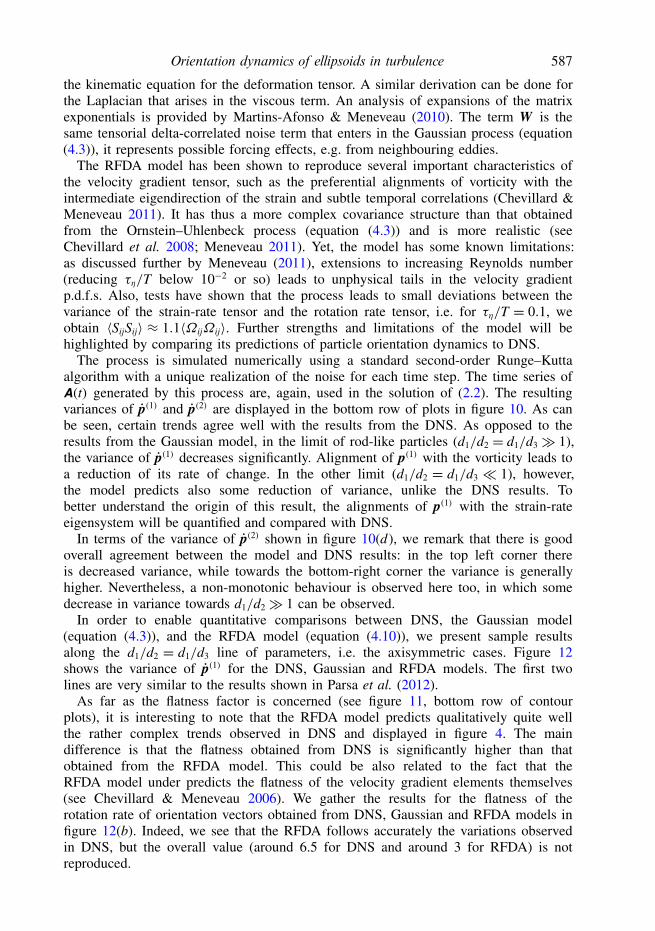
As far as the flatness factor is concerned (see figure 11, bottom row of contourplots), it is interesting to note that the RFDA model predicts qualitatively quite wellthe rather complex trends observed in DNS and displayed in figure 4. The maindifference is that the flatness obtained from DNS is significantly higher than thatobtained from the RFDA model. This could be also related to the fact that theRFDA model under predicts the flatness of the velocity gradient elements themselves(see Chevillard & Meneveau 2006). We gather the results for the flatness of therotation rate of orientation vectors obtained from DNS, Gaussian and RFDA models infigure 12(b). Indeed, we see that the RFDA follows accurately the variations observedin DNS, but the overall value (around 6.5 for DNS and around 3 for RFDA) is notreproduced.


0.10

0.15

0.20

0.25

–2 –1 0 1 2

2

3

4

5

6

7

–2 –1 0 1 2

(b)(a)

FIGURE 12. Variance (a) and flatness factor (b) of p(1) from DNS (solid line), theGaussian model (dot-dashed) and the RFDA model (dashed line). We added also theprediction equation (4.2) (dotted line) assuming that p(i) and velocity gradients are statisticallyindependent.

Analysis of model predictions of orientations of p(1) for axisymmetric particles(i.e. d1/d2 = d1/d3) with vorticity and strain-rate eigenvectors leads to the resultsshown in figures 13 and 14, for both Gaussian and RFDA models.

For the Gaussian model, no preferential alignments of p(1) with vorticity canbe observed. Results for alignment with the strain eigenframe show a strongpreferential alignment of fibre-like particles with the eigenvector associated withthe most extensive eigendirection, no preferential alignments with the intermediateeigendirection and preferential alignments of disc-like particles with the mostcontracting eigendirection. This numerical study reveals indeed, for this Gaussianmodel (equation (4.3)), a correlation between orientation vectors and velocity gradients,although of different nature as that observed in DNS: whereas preferential alignmentsof fibre-like particles with intermediate eigendirection and disc-like particle with mostcontracting one are found in DNS, Gaussian process only correctly predicts alignmentsof disc-like particles with most-contracting eigendirection and reveals non-realisticalignment properties of fibres.

More refined Gaussian processes have been proposed for velocity gradient statistics.For instance, Pumir & Wilkinson (2011) and Vincenzi (2013) have considered anOrnstein–Uhlenbeck process for A with different correlation time scales for thesymmetric and antisymmetric parts. This is more realistic, since it is known thatin turbulence the correlation time scale for the rotation rate is significantly longerthan that of the strain rate. Applying this stochastic model to the orientation dynamicsof rods (i.e. with d1/d2 = d1/d3→∞), Pumir & Wilkinson (2011) observe similarlya strong preferential alignment of p with the strain eigenvector associated with themost positive eigenvalue. This differs from the observations in DNS (see figures 5and 6), where p is instead found to be preferentially aligned with the direction ofvorticity. As argued before, such trends then have immediate implications on theparticle rotation rates. These results and arguments highlight the importance of boththe temporal and alignment structure of A. Similar conclusions have been arrived atrecently by Gustavsson, Einarsson & Mehlig (2013) who consider also the case of


Gau

ssia

n

RFD

A

1.0

0.5

01.0

0.5

0

0.2

0.4

0.6

0.8

1.0

1.2

0.2

0.4

0.6

0.8

1.0

1.2

–2 –1 0 1 2

(a)

(b)

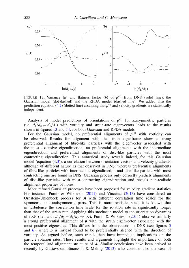
FIGURE 13. (Colour online) P.d.f. of the cosine of the angle between the vorticity directionω and the ellipsoid’s major axis p(1) for the axisymmetric case, as a function of the anisotropyparameter α = d1/d3 = d1/d2). (a) Gaussian stochastic model (see § 4.2), for which thealignment appears flat, for any ellipsoidal aspect ratios. (b) Results from RFDA Lagrangianstochastic model. Contour lines correspond to values 0.4, 0.6, 0.8, 1, 1.2.

inertial axisymmetric particles and obtained analytical expressions for the rotation rateassuming an underlying Gaussian flow.

The alignments predicted by the RFDA model are significantly more realistic: as canbe seen, for fibre-like particles (d1/d2→∞), the model predicts strong alignment withvorticity (figure 13b). In the other limit, for disc-like particles, p(1) in the model ispreferentially perpendicular to the vorticity. That is to say, the vorticity is in the planeof the disc. Nevertheless, comparing in more detail with the DNS results in figure 5, itis evident that the model predicts a significantly broader (and weaker) alignment peakin the p.d.f. (see the different magnitudes given in colourbars). Hence, the alignment


1.0

0.5

01.0

0.5

0–2 –1 0 1 2 –2 –1 0 1 2 –2 –1 0 1 2

0.5

1.0

1.5

0.5

1.0

1.5

2.0

2.5

RFD

AG

auss

ian

(a)

(b)

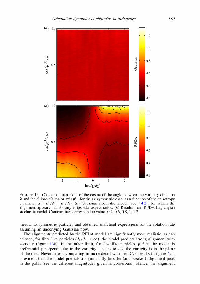
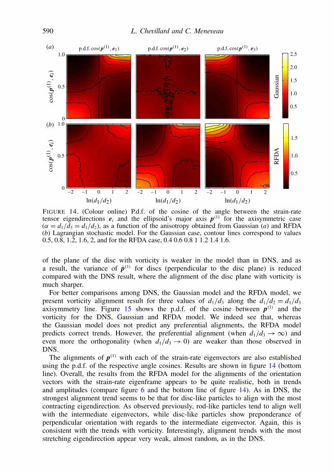
FIGURE 14. (Colour online) P.d.f. of the cosine of the angle between the strain-ratetensor eigendirections ei and the ellipsoid’s major axis p(1) for the axisymmetric case(α = d1/d3 = d1/d2), as a function of the anisotropy obtained from Gaussian (a) and RFDA(b) Lagrangian stochastic model. For the Gaussian case, contour lines correspond to values0.5, 0.8, 1.2, 1.6, 2, and for the RFDA case, 0.4 0.6 0.8 1 1.2 1.4 1.6.

of the plane of the disc with vorticity is weaker in the model than in DNS, and asa result, the variance of p(1) for discs (perpendicular to the disc plane) is reducedcompared with the DNS result, where the alignment of the disc plane with vorticity ismuch sharper.

For better comparisons among DNS, the Gaussian model and the RFDA model, wepresent vorticity alignment result for three values of d1/d3 along the d1/d2 = d1/d3

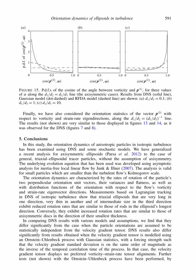
axisymmetry line. Figure 15 shows the p.d.f. of the cosine between p(1) and thevorticity for the DNS, Gaussian and RFDA model. We indeed see that, whereasthe Gaussian model does not predict any preferential alignments, the RFDA modelpredicts correct trends. However, the preferential alignment (when d1/d3 →∞) andeven more the orthogonality (when d1/d3 → 0) are weaker than those observed inDNS.

The alignments of p(1) with each of the strain-rate eigenvectors are also establishedusing the p.d.f. of the respective angle cosines. Results are shown in figure 14 (bottomline). Overall, the results from the RFDA model for the alignments of the orientationvectors with the strain-rate eigenframe appears to be quite realistic, both in trendsand amplitudes (compare figure 6 and the bottom line of figure 14). As in DNS, thestrongest alignment trend seems to be that for disc-like particles to align with the mostcontracting eigendirection. As observed previously, rod-like particles tend to align wellwith the intermediate eigenvectors, while disc-like particles show preponderance ofperpendicular orientation with regards to the intermediate eigenvector. Again, this isconsistent with the trends with vorticity. Interestingly, alignment trends with the moststretching eigendirection appear very weak, almost random, as in the DNS.


1

2

3

0.5 1.0 0 0.5 1.0 0 0.5 1.00

4(a) (b) (c)

FIGURE 15. P.d.f.s of the cosine of the angle between vorticity and p(1), for three valuesof α along the d1/d2 = d1/d3 line (the axisymmetric cases). Results from DNS (solid line),Gaussian model (dot-dashed) and RFDA model (dashed line) are shown: (a) d1/d3 = 0.1; (b)d1/d3 = 1; (c) d1/d3 = 10.

Finally, we have also considered the orientation statistics of the vector p(2) withrespect to vorticity and strain-rate eigendirections, along the d1/d2 = (d1/d3)

−1 line.The results (not shown) are very similar to those displayed in figures 13 and 14, as itwas observed for the DNS (figures 7 and 8).

5. ConclusionsIn this study, the orientation dynamics of anisotropic particles in isotropic turbulence

has been examined using DNS and some stochastic models. We have generalizeda recent analysis for axisymmetric ellipsoids (Parsa et al. 2012) to the case ofgeneral, triaxial–ellipsoidal tracer particles, without the assumption of axisymmetry.The underlying evolution equation that has been used was developed using asymptoticanalysis for inertia-free local linear flow by Junk & Illner (2007). The analysis is validfor small particles which are smaller than the turbulent flow’s Kolmogorov scale.

The orientation dynamics are characterized by the rates of rotation of the particle’stwo perpendicular orientation unit vectors, their variances and flatness, as well aswith distribution functions of the orientation with respect to the flow’s vorticityand strain-rate eigenvector directions. Measurements based on Lagrangian trackingin DNS of isotropic turbulence show that triaxial ellipsoids that are very long inone direction, very thin in another and of intermediate size in the third directionexhibit reduced rotation rates that are similar to those of rods in the ellipsoid’s longestdirection. Conversely, they exhibit increased rotation rates that are similar to those ofaxisymmetric discs in the direction of their smallest thickness.

In comparing DNS results with various models and assumptions, we find that theydiffer significantly from the case when the particle orientations are assumed to bestatistically independent from the velocity gradient tensor. DNS results also differsignificantly from results obtained when the velocity gradient tensor is modelled usingan Ornstein–Uhlenbeck process with Gaussian statistics, with a forcing strength suchthat the velocity gradient standard deviation is on the same order of magnitude asthe inverse of the temporal correlation time of the process. In that case, the velocitygradient tensor displays no preferred vorticity–strain-rate tensor alignments. Furthertests (not shown) with the Ornstein–Uhlenbeck process have been performed, by


varying the strength of the forcing. It is observed that when the forcing strengthis reduced from the baseline (high) values (i.e. ∼1/τ 3/2

η ) to values of the order of1/T3/2 (or unity, when using units of T , as was the case for the RFDA model) whilemaintaining the correlation time fixed at τη, then the results tend to those obtainedassuming statistical independence among orientation vectors and the velocity gradienttensor. The fact that the two approaches lead to the same result can be understoodas follows: the dimensionless quantities V (i) may only depend on dimensionlessparameters. One of these is, e.g., θ = τη〈ΩijΩij〉1/2, a combination of the processcorrelation time scale τη and the velocity gradient variance. Hence, reducing theforcing strength in the Gaussian process, i.e. letting 〈ΩijΩij〉 → 0 while keeping τηfixed implies θ → 0. This same limit may be achieved by keeping the variancefixed but reducing the correlation time scale τη → 0. When the correlation timescale of the velocity gradient tensor tends to zero, one expects the same results asassuming statistical independence between the orientation vectors and the velocitygradient tensor.

DNS results are also compared with a stochastic model for the velocity gradienttensor in which the pressure and viscous effects are modelled based on the RFDA.We remark that in the RFDA model, the nonlinear terms cause a large velocitygradient variance (finite θ ) even when the forcing strength is weak. Thus, in theRFDA model the variance and the correlation time are linked and cannot be controlledindependently as they can be in the Ornstein–Uhlenbeck model. Unlike the Gaussianlinear model, the RFDA-based stochastic model accurately predicts the reduction inrotation rate in the longest direction of triaxial ellipsoids. This is due to the fact thatthis direction aligns well with the flow’s vorticity, with its rotation perpendicular tothe vorticity thus being reduced. For disc-like particles, or in directions perpendicularto the longest direction in triaxial particles, the model predicts smaller rotation ratesthan those observed in DNS (although still larger than for rods). This behaviourhas been explained based on the probability of vorticity orientation with the mostcontracting strain-rate eigendirection. In DNS, this alignment is very likely (sharppeak in the p.d.f.), whereas the peak in the p.d.f. predicted by the model is morediffused. Furthermore, the RFDA model falls short at reproducing the high flatness ofthe rotation rate amplitude (i.e. pipi, see figure 12b), although trends (exceeding theGaussian values) are consistent. The under-prediction of flatness is likely due to thefact that the model does not reproduce the intermittent peak values of the velocitygradient components themselves (see Chevillard & Meneveau 2006) in which thehigh-intensity tails of the velocity gradient elements can be seen to fall off faster thanthose in DNS. Present results point to the need for further improvements in stochasticLagrangian models for the velocity gradient tensor. Specifically, a model that predictsa sharper alignment between vorticity in a plane perpendicular to the most contractingstrain-rate eigendirection would be expected to lead to a more accurate prediction ofthe increased rotation rates of discs.

The deformation and breakup of viscous drops in shear flows are greatly affectedby the Lagrangian properties of fluid velocity gradients (Stone 1994). In some cases,it is possible to assume droplets are of ellipsoidal shape, as was done for exampleby Mosler & Shaqfeh (1997) and Maffettone & Minale (1998), or even allowingfor more non-trivial shape deformations (Cristini et al. 2003). In either case, non-trivial correlations among the drop deformations and the strain eigendirections andvorticity of the flow suggest that turbulence will affect the rotation (tumbling) rates ofdeforming particles differently than is the case for rigid particles. Exploration of theRFDA model in the context of deforming particles is left for future studies.


AcknowledgementsThe authors thank Emmanuel Leveque for providing the authors with the Lagrangian

time series of velocity gradient tensor from DNS, B. Castaing and A. Prosperettifor fruitful discussions, D. Bartolo on plotting issues. C.M. thanks the Laboratoirede Physique de l’Ecole Normale Superieure de Lyon for their hospitality during asabbatical stay and the US National Science Foundation (grant # CBET-1033942)for support of turbulence research. We also thank the PSMN (ENS Lyon) forcomputational resources.

Appendix. Calculation of the variance of rotation rates for the independentcase

In this section, we present the calculation of V (i) = 〈p(i) · p(i)〉 for the case when it isassumed that p(i), for any i = 1, 2, 3, is statistically independent of the strain-rate androtation tensors. We furthermore assume that each p(i) is an isotropic vector, and recallthat the set of vectors (p(1), p(2), p(3)) is an orthonormal basis. For this purpose, eachside of the Junke–Illner equation (see (2.4)) is squared and averaged:

〈p(i)n p(i)n 〉 =⟨(

Ωnjp(i)j +

∑k,m


(i)l

)

×(Ωngp(i)g +

∑a,b

εiabλ(b)p(a)n p(a)r Srsp

(i)s

)⟩. (A 1)

Expanding and using the assumption of statistical independence between p, S and Ω ,the following expressions must be evaluated:

〈Ωnjp(i)j Ωngp(i)g 〉 = 〈ΩnjΩng〉〈p(i)j p(i)g 〉, (A 2)

2

⟨Ωnjp

(i)j

∑a,b


(i)s

⟩= 2〈ΩnjSrs〉

∑a,b

εiabλ(b)〈p(i)j p(i)s p(a)n p(a)r 〉, (A 3)

and ⟨∑k,m


(i)l

∑a,b


(i)s

⟩

= 〈SqlSrs〉∑k,m

∑a,b

εikmεiabλ(m)λ(b)〈p(k)n p(a)n p(k)q p(a)r p(i)l p(i)s 〉. (A 4)

The set of vectors (p(1), p(2), p(3)) is an orthonormal basis, thus

p(k)n p(a)n = δka. (A 5)

This implies that (A 4) simplifies to⟨∑k,m


(i)l

∑a,b


(i)s

⟩

= 〈SqlSrs〉∑m,b,k

εikmεikbλ(m)λ(b)〈p(k)q p(k)r p(i)l p(i)s 〉. (A 6)


We can see that the average of |p(i)|2 (equation (A 1)) depends only on the statisticsof velocity gradients and second and fourth moments of orientation vector components.Assumption of isotropy for the unit vectors p(i) implies that

〈p(i)j p(i)g 〉 = 13δjg, (A 7)

〈p(k)q p(k)r p(i)l p(i)s 〉 = A(k,i)δqrδls + B(k,i)δqlδrs + C(k,i)δqsδrl. (A 8)

From there it is easily seen that (A 3) gives no contributions since any contractions ofΩnjSrs vanish. The three remaining unknown coefficients that enter in the evaluation of(A 6) may be found by specifying particular values. For instance, the index contractionq= r and l= s yields

〈p(k)q p(k)q p(i)l p(i)l 〉 = 〈1× 1〉 = 1= 9A(k,i) + 3B(k,i) + 3C(k,i). (A 9)

Inspecting (A 6), we note that terms in the sum such that k = i give no contributionbecause of the εikmεikb. Thus, we consider k 6= i. In this case, the contraction q = l andr = s yields

0= 3A(k,i) + 9B(k,i) + 3C(k,i), (A 10)

and the contraction q= s and r = l yields

0= 3A(k,i) + 3B(k,i) + 9C(k,i). (A 11)

Solving these equations yields in the case k 6= i

A(k,i) = 215 and B(i,a) = C(i,a) =− 1

30 . (A 12)

Finally, simplifying (A 2) with (A 7) and contracting the isotropic form (A 8) with〈SqlSrs〉, we obtain

〈|p(i)|2〉 = 13〈ΩpqΩpq〉 + 1

10〈SpqSpq〉

∑m,b,k 6=i

εikmεikbλ(m)λ(b). (A 13)

Using the isotropic relations 〈ΩpqΩpq〉 = 〈SpqSpq〉 and normalizing the former relationby 2〈ΩpqΩpq〉 = ε/ν, we get the following functional forms for the fluctuation ofrotation rate variances:

V (i)SI =

16+ 1

20

∑k 6=i

(λ(k))2. (A 14)

If furthermore the statistics of A are assumed Gaussian (as in § 4.2), it is alsopossible to derive exactly the value for the flatness, although the calculation is moretedious. For the particular case of spheres, i.e. d1 = d2 = d3 or λ(i) = 0, the dynamics israther simple since p(i)n =Ωnjp

(i)j . Assuming that p(i) is isotropic and independent on A,

we easily obtain 〈|p(i)|4〉 = [〈tr2ΩΩ>〉 + 2〈tr(ΩΩ>)2〉]/15. For isotropic, homogeneousand trace-free Gaussian velocity gradient tensors, we obtain 〈tr2ΩΩ>〉 = 5〈trΩΩ>〉2/3and 〈tr(ΩΩ>)2〉 = 5〈trΩΩ>〉2/6. Since, 〈|p(i)|2〉 = 〈trΩΩ>〉/3, we finally obtain

F(i)SI (1, 1)= 2. (A 15)


R E F E R E N C E S

ASHURST, W. T., KERSTEIN, R., KERR, R. & GIBSON, C. 1987 Alignment of vorticity andscalar gradient with the strain rate in simulated Navier–Stokes turbulence. Phys. Fluids 30,2343–2353.

BERNSTEIN, O. & SHAPIRO, M. 1994 Direct determination of the orientation distribution functionof cylindrical particles immersed in laminar and turbulent shear flows. J. Aerosol Sci. 25,113–136.

BIFERALE, L., CHEVILLARD, L., MENEVEAU, C. & TOSCHI, F. 2007 Multiscale model of gradientevolution in turbulent flows. Phys. Rev. Lett. 98, 214501.

BRETHERTON, F. P. 1962 The motion of rigid particles in a shear flow at low Reynolds number.J. Fluid Mech. 14, 284–304.

BRUNK, B. K., KOCH, D. L. & LION, L. W. 1998 A model for alignment between microscopicrods and vorticity. J. Fluid Mech. 364, 81–113.

CANTWELL, B. J. 1992 Exact solution of a restricted Euler equation for the velocity gradient tensor.Phys. Fluids A 4, 782–793.

CHERTKOV, M., PUMIR, A. & SHRAIMAN, B. I. 1999 Lagrangian tetrad dynamics and thephenomonology of turbulence. Phys. Fluids 11, 2394–2410.

CHEVILLARD, L., MENEVEAU, C., BIFERALE, L. & TOSCHI, F. 2008 Modelling the pressureHessian and viscous Laplacian in turbulence: comparisons with direct numerical simulationand implications on velocity gradient dynamics. Phys. Fluids 20, 101504.

CHEVILLARD, L. & MENEVEAU, C. 2006 Lagrangian dynamics and statistical geometric structure ofturbulence. Phys. Rev. Lett. 97, 174501.

CHEVILLARD, L. & MENEVEAU, C. 2007 Intermittency and universality in a Lagrangian model ofvelocity gradients in three-dimensional turbulence. C. R. Mec. 335, 187–193.

CHEVILLARD, L. & MENEVEAU, C. 2011 Lagrangian time correlations of vorticity alignments inisotropic turbulence: observations and model predictions. Phys. Fluids 23, 101704.

CRISTINI, V., BLAWZDZIEWICZ, J. B., LOEWENBERG, M. & COLLINS, L. R. 2003 Breakup instochastic Stokes flows: sub-Kolmogorov drops in isotropic turbulence. J. Fluid Mech. 492,231–250.

GIERSZEWSKI, P. J. & CHAFFEY, C. E. 1978 Rotation of an isolated triaxial ellipsoid suspended inslow viscous flow. Canad. J. Phys. 56, 6–11.

GIRIMAJI, S. S. & POPE, S. B. 1990a A diffusion model for velocity gradients in turbulence. Phys.Fluids A 2, 242–256.

GIRIMAJI, S. S. & POPE, S. B. 1990b Material element deformation in isotropic turbulence.J. Fluid Mech. 220, 427–458.

GONZALEZ, M. 2009 Kinematic properties of passive scalar gradient predicted by a stochasticLagrangian model. Phys. Fluids 21, 055104.

GUSTAVSSON, K., EINARSSON, J. & MEHLIG, B. 2013 Tumbling of small axisymmetric particles inrandom and turbulent flows. Preprint arXiv: 1305.1822.

HATER, T., HOMANN, H. & GRAUER, R. 2011 Lagrangian model for the evolution of turbulentmagnetic and passive scalar fields. Phys. Rev. E 83, 017302.

HINCH, E. J. & LEAL, L. G. 1979 Rotation of small non-axisymmetric particles in a simple shearflow. J. Fluid Mech. 92, 591.

JEFFERY, G. B. 1922 The motion of ellipsoidal particles immersed in a viscous fluid. Proc. R. Soc.Lond. A 102, 161–179.

JEONG, E. & GIRIMAJI, S. S. 2003 Velocity-gradient dynamics in turbulence: effect of viscosity andforcing. Theor. Comput. Fluid Dyn. 16, 421–432.

JUNK, M. & ILLNER, R. 2007 A new derivation of Jeffery’s equation. J. Math. Fluid Mech. 9,455–488.

KOCH, D. L. & SUBRAMANIAN, G. R. 2011 Collective hydrodynamics of swimmingmicroorganisms: living fluids. Annu. Rev. Fluid Mech. 434, 637–659.

LARSON, R. G. 1999 The Structure and Rheology of Complex Fluid. Oxford University Press.LI, Y 2011 Small-scale intermittency and local anisotropy in turbulent mixing with rotation.

J. Turbul. 12, N38.

http://arxiv.org/abs/1305.1822










LUNDELL, F., SODERBERG, D. L. & ALFREDSSON, H. P. 2011 Fluid mechanics of papermaking.Annu. Rev. Fluid Mech. 43, 195.

MAFFETTONE, P. L. & MINALE, M. 1998 Equation of change for ellipsoidal drops in viscous flow.J. Non-Newtonian Fluid Mech. 78, 227–241.

MARTINS-AFONSO, M. & MENEVEAU, C. 2010 Recent fluid deformation closure for velocitygradient tensor dynamics in turbulence: timescale effects and expansions. Physica D 239,1241–1250.

MENEVEAU, C. 2011 Lagrangian dynamics and models of the velocity gradient tensor in turbulentflows. Annu. Rev. Fluid Mech. 43, 219–245.

MORTENSEN, P. H., ANDERSON, H. I., GILLISSEN, J. J. J. & BOERSMA, B. J. 2008 Dynamics ofprolate ellipsoidal particles in a turbulent channel flow. Phys. Fluids 20, 093302.

MOSLER, A. B. & SHAQFEH, E. S. G. 1997 Drop breakup in the flow through fixed beds viastochastic simulation in model Gaussian fields. Phys. Fluids 9, 3209.

NASO, A., PUMIR, A. & CHERTKOV, M. 2007 Statistical geometry in homogeneous and isotropicturbulence. J. Turbul. 8, N. 39.

NEWSOM, R. K. & BRUCE, C. W. 1998 Orientational properties of fibrous aerosols in atmosphericturbulence. J. Aerosol Sci. 29, 773–797.

PARSA, S., CALZAVARINI, E., TOSCHI, F. & VOTH, G. A. 2012 Rotation rate of rods in turbulentfluid flow. Phys. Rev. Lett. 109, 134501.

PEDLEY, T. J. & KESSLER, J. O. 1992 Hydrodynamic phenomena in suspensions of swimmingmicroorganisms. Annu. Rev. Fluid Mech. 24, 313–358.

PINSKY, M. B. & KHAIN, A. P. 1998 Some effects of cloud turbulence on water–ice and ice–icecollisions. Atmos. Res. 47–48, 69–86.

PUMIR, A. & WILKINSON, M. 2011 Orientation statistics of small particles in turbulence. New J.Phys. 13, 0930306.

SAINTILLAN, D. & SHELLEY, M. J. 2007 Orientational order and instabilities in suspensions ofself-locomoting rods. Phys. Rev. Lett. 99, 058102.

SHIN, M. & KOCH, D. L. 2005 Rotational and translational dispersion of fibres in isotropicturbulent flows. J. Fluid Mech. 540, 143–173.

STONE, H. A. 1994 Dynamics of drop deformation and breakup in viscous fluids. Annu. Rev. FluidMech. 26, 65–102.

VINCENZI, D. 2013 Orientation of non-spherical particles in an axisymmetric random flow. J. FluidMech. 719, 465–487.

WILKINSON, M. & KENNARD, H. R. 2012 A model for alignment between microscopic rods andvorticity. J. Phys. A: Math. Theor. 45, 455502.

YARIN, A. L., GOTTLIEB, O. & ROISMAN, I. V 1997 Chaotic rotation of triaxial ellipsoids insimple shear flow. J. Fluid Mech. 340, 83–100.

ZHANG, H., AHMADI, G., FAN, F. G. & MCLAUGHLIN, J. B. 2001 Ellipsoidal particles transportand deposition in turbulent channel flows. Intl. J. Multiphase Flow 27, 971–1009.

ZIMMERMANN, R., GASTEUIL, Y., BOURGOIN, M., VOLK, R., PUMIR, A. & PINTON, J.-F.2011 Rotational intermittency and turbulence induced lift experienced by large particles in aturbulent flow. Phys. Rev. Lett. 106, 154501.

Documents

J. Fluid Mech. (2013), . 737, pp. doi:10.1017/jfm.2013.580 ...perso.ens-lyon.fr/laurent.chevillard/MyPageFiles/Jfm737.pdf · special case of an axisymmetric ellipsoid, the evolution