Embed Size (px)
Citation preview
It’s All in the Hidden States:A Hedging Method with an Explicit Measure of
Population Basis RiskYanxin Liu and Johnny Siu-Hang Li
Presenter: Yanxin Liu
September 9, 2015
Presenter: Yanxin Liu It’s All in the Hidden States: A Hedging Method with an Explicit Measure of Population Basis RiskSeptember 9, 2015 1 / 44

Outline
1 Introduction
2 The Applicable Mortality Models
3 The Generalized State Space Hedging Method
4 Analyzing Population Basis Risk
5 A Numerical Illustration
6 Conclusion
Presenter: Yanxin Liu It’s All in the Hidden States: A Hedging Method with an Explicit Measure of Population Basis RiskSeptember 9, 2015 2 / 44
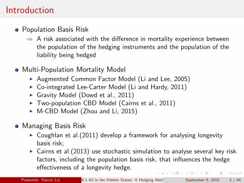
Introduction
Population Basis Risk⇒ A risk associated with the difference in mortality experience between
the population of the hedging instruments and the population of theliability being hedged
Multi-Population Mortality ModelI Augmented Common Factor Model (Li and Lee, 2005)I Co-integrated Lee-Carter Model (Li and Hardy, 2011)I Gravity Model (Dowd et al., 2011)I Two-population CBD Model (Cairns et al., 2011)I M-CBD Model (Zhou and Li, 2015)
Managing Basis RiskI Coughlan et al.(2011) develop a framework for analysing longevity
basis risk;I Cairns et al.(2013) use stochastic simulation to analyse several key risk
factors, including the population basis risk, that influences the hedgeeffectiveness of a longevity hedge.
Presenter: Yanxin Liu It’s All in the Hidden States: A Hedging Method with an Explicit Measure of Population Basis RiskSeptember 9, 2015 3 / 44
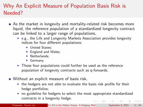
Why An Explicit Measure of Population Basis Risk isNeeded?
As the market in longevity and mortality-related risk becomes moreliquid, the reference population of a standardized longevity contractcan be linked to a larger range of populations,
I e.g., the Life and Longevity Markets Association provides longevityindices for four different populations:
F United States;F England and Wales;F Netherlands;F Germany.
I Those four populations could further be used as the referencepopulation of longevity contracts such as q-forwards.
Without an explicit measure of basis risk,I the hedgers are not able to evaluate the basis risk profile for their
hedge portfolios;I no guideline for hedgers to select the most appropriate standardized
contracts in a longevity hedge.
Presenter: Yanxin Liu It’s All in the Hidden States: A Hedging Method with an Explicit Measure of Population Basis RiskSeptember 9, 2015 4 / 44
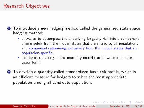
Research Objectives
1 To introduce a new hedging method called the generalized state spacehedging method;
I allows us to decompose the underlying longevity risk into a componentarising solely from the hidden states that are shared by all populationsand components stemming exclusively from the hidden states that arepopulation-specific.
I can be used as long as the mortality model can be written in statespace form;
2 To develop a quantity called standardized basis risk profile, which isan efficient measure for hedgers to select the most appropriatepopulation among all candidate populations.
Presenter: Yanxin Liu It’s All in the Hidden States: A Hedging Method with an Explicit Measure of Population Basis RiskSeptember 9, 2015 5 / 44

Outline
1 Introduction
2 The Applicable Mortality Models
3 The Generalized State Space Hedging Method
4 Analyzing Population Basis Risk
5 A Numerical Illustration
6 Conclusion
Presenter: Yanxin Liu It’s All in the Hidden States: A Hedging Method with an Explicit Measure of Population Basis RiskSeptember 9, 2015 6 / 44
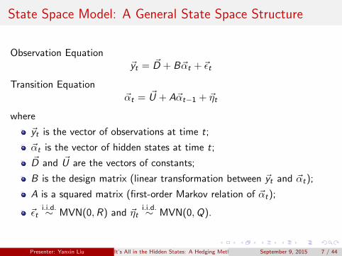
State Space Model: A General State Space Structure
Observation Equation~yt = ~D + B~αt + ~εt
Transition Equation~αt = ~U + A~αt−1 + ~ηt
where
~yt is the vector of observations at time t;
~αt is the vector of hidden states at time t;~D and ~U are the vectors of constants;
B is the design matrix (linear transformation between ~yt and ~αt);
A is a squared matrix (first-order Markov relation of ~αt);
~εti.i.d.∼ MVN(0,R) and ~ηt
i.i.d.∼ MVN(0,Q).
Presenter: Yanxin Liu It’s All in the Hidden States: A Hedging Method with an Explicit Measure of Population Basis RiskSeptember 9, 2015 7 / 44
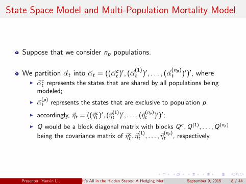
State Space Model and Multi-Population Mortality Model
Suppose that we consider np populations.
We partition ~αt into ~αt = ((~αct )′, (~α
(1)t )′, . . . , (~α
(np)t )′)′, where
I ~αct represents the states that are shared by all populations being
modeled;
I ~α(p)t represents the states that are exclusive to population p.
I accordingly, ~ηt = ((~ηct )′, (~η(1)t )′, . . . , (~η
(np)t )′)′;
I Q would be a block diagonal matrix with blocks Qc ,Q(1), . . . ,Q(np)
being the covariance matrix of ~ηct , ~η(1)t , . . . , ~η
(np)t , respectively.
Presenter: Yanxin Liu It’s All in the Hidden States: A Hedging Method with an Explicit Measure of Population Basis RiskSeptember 9, 2015 8 / 44
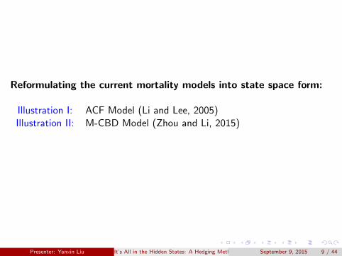
Reformulating the current mortality models into state space form:
Illustration I: ACF Model (Li and Lee, 2005)Illustration II: M-CBD Model (Zhou and Li, 2015)
Presenter: Yanxin Liu It’s All in the Hidden States: A Hedging Method with an Explicit Measure of Population Basis RiskSeptember 9, 2015 9 / 44
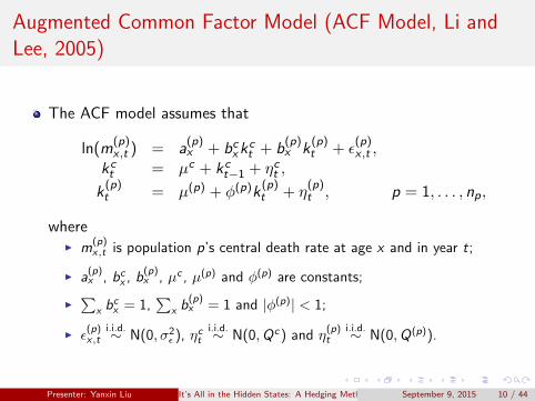
Augmented Common Factor Model (ACF Model, Li andLee, 2005)
The ACF model assumes that
ln(m(p)x ,t ) = a
(p)x + bcxk
ct + b
(p)x k
(p)t + ε
(p)x ,t ,
kct = µc + kct−1 + ηct ,
k(p)t = µ(p) + φ(p)k
(p)t + η
(p)t , p = 1, . . . , np,
whereI m
(p)x,t is population p’s central death rate at age x and in year t;
I a(p)x , bcx , b
(p)x , µc , µ(p) and φ(p) are constants;
I∑
x bcx = 1,
∑x b
(p)x = 1 and |φ(p)| < 1;
I ε(p)x,t
i.i.d.∼ N(0, σ2ε ), ηct
i.i.d.∼ N(0,Qc) and η(p)t
i.i.d.∼ N(0,Q(p)).
Presenter: Yanxin Liu It’s All in the Hidden States: A Hedging Method with an Explicit Measure of Population Basis RiskSeptember 9, 2015 10 / 44
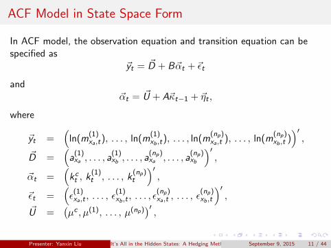
ACF Model in State Space Form
In ACF model, the observation equation and transition equation can bespecified as
~yt = ~D + B~αt + ~εt
and~αt = ~U + A~κt−1 + ~ηt ,
where
~yt =(
ln(m(1)xa,t), . . . , ln(m
(1)xb,t), . . . , ln(m
(np)xa,t ), . . . , ln(m
(np)xb,t )
)′,
~D =(a
(1)xa , . . . , a
(1)xb , . . . , a
(np)xa , . . . , a
(np)xb
)′,
~αt =(kct , k
(1)t , . . . , k
(np)t
)′,
~εt =(ε
(1)xa,t , . . . , ε
(1)xb,t , . . . , ε
(np)xa,t , . . . , ε
(np)xb,t
)′,
~U =(µc , µ(1), . . . , µ(np)
)′,
Presenter: Yanxin Liu It’s All in the Hidden States: A Hedging Method with an Explicit Measure of Population Basis RiskSeptember 9, 2015 11 / 44
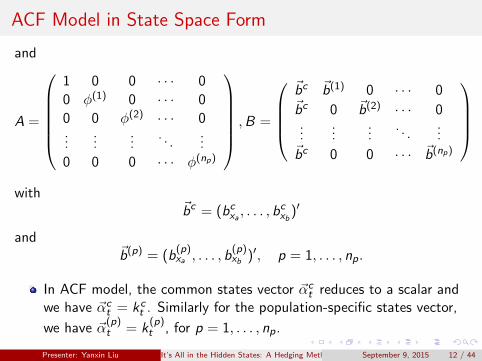
ACF Model in State Space Form
and
A =
1 0 0 · · · 0
0 φ(1) 0 · · · 0
0 0 φ(2) · · · 0...
......
. . ....
0 0 0 · · · φ(np)
,B =
~bc ~b(1) 0 · · · 0~bc 0 ~b(2) · · · 0...
......
. . ....
~bc 0 0 · · · ~b(np)
with
~bc = (bcxa , . . . , bcxb
)′
and~b(p) = (b
(p)xa , . . . , b
(p)xb )′, p = 1, . . . , np.
In ACF model, the common states vector ~αct reduces to a scalar and
we have ~αct = kct . Similarly for the population-specific states vector,
we have ~α(p)t = k
(p)t , for p = 1, . . . , np.
Presenter: Yanxin Liu It’s All in the Hidden States: A Hedging Method with an Explicit Measure of Population Basis RiskSeptember 9, 2015 12 / 44
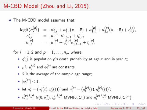
M-CBD Model (Zhou and Li, 2015)
The M-CBD model assumes that
logit(q(p)x ,t ) = κc1,t + κc2,t(x − x) + κ
(p)1,t + κ
(p)2,t (x − x) + ε
(p)x ,t ,
κci ,t = µci + κci ,t−1 + ηci ,t ,
κ(p)i ,t = µ
(p)i + φ
(p)i κ
(p)i ,t−1 + η
(p)i ,t ,
for i = 1, 2 and p = 1, . . . , np, where
I q(p)x,t is population p’s death probability at age x and in year t;;
I µci , µ
(p)i and φ
(p)i are constants;
I x is the average of the sample age range;
I |φ(p)i | < 1;
I let ~ηct = (ηc1(t), ηc2(t))′ and ~η(p)t = (η
(p)1 (t), η
(p)2 (t))′;
I ε(p)x,t
i.i.d.∼ N(0, σ2ε ), ~ηct
i.i.d.∼ MVN(0,Qc) and ~η(p)t
i.i.d.∼ MVN(0,Q(p)).
Presenter: Yanxin Liu It’s All in the Hidden States: A Hedging Method with an Explicit Measure of Population Basis RiskSeptember 9, 2015 13 / 44
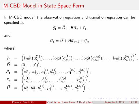
M-CBD Model in State Space Form
In M-CBD model, the observation equation and transition equation can bespecified as
~yt = ~D + B~αt + ~εt
and~αt = ~U + A~κt−1 + ~ηt ,
where
~yt =(logit(q
(1)xa,t), . . . , logit(q
(1)xb,t), . . . , logit(q
(np)xa,t ), . . . , logit(q
(np)xb,t )
)′,
~D = (0, . . . , 0)′ ,
~αt =(κc1,t , κ
c2,t , κ
(1)1,t , κ
(1)2,t , . . . , κ
(np)1,t , κ
(np)2,t
)′,
~εt =(ε
(1)xa,t , . . . , ε
(1)xb,t , . . . , ε
(np)xa,t , . . . , ε
(np)xb,t
)′,
~U =(µc1, µ
c2, µ
(1)1 , µ
(1)2 . . . , µ
(np)1 , µ
(np)2
)′,
Presenter: Yanxin Liu It’s All in the Hidden States: A Hedging Method with an Explicit Measure of Population Basis RiskSeptember 9, 2015 14 / 44
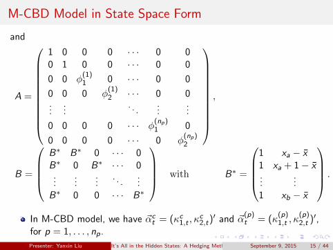
M-CBD Model in State Space Form
and
A =
1 0 0 0 · · · 0 00 1 0 0 · · · 0 0
0 0 φ(1)1 0 · · · 0 0
0 0 0 φ(1)2 · · · 0 0
......
. . ....
...
0 0 0 0 · · · φ(np)1 0
0 0 0 0 · · · 0 φ(np)2
,
B =
B∗ B∗ 0 · · · 0B∗ 0 B∗ · · · 0...
......
. . ....
B∗ 0 0 · · · B∗
with B∗ =
1 xa − x1 xa + 1− x...
...1 xb − x
.
In M-CBD model, we have ~αct = (κc1,t , κ
c2,t)′ and ~α
(p)t = (κ
(p)1,t , κ
(p)2,t )′,
for p = 1, . . . , np.
Presenter: Yanxin Liu It’s All in the Hidden States: A Hedging Method with an Explicit Measure of Population Basis RiskSeptember 9, 2015 15 / 44

Outline
1 Introduction
2 The Applicable Mortality Models
3 The Generalized State Space Hedging Method
4 Analyzing Population Basis Risk
5 A Numerical Illustration
6 Conclusion
Presenter: Yanxin Liu It’s All in the Hidden States: A Hedging Method with an Explicit Measure of Population Basis RiskSeptember 9, 2015 16 / 44
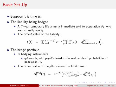
Basic Set Up
Suppose it is time t0.
The liability being hedgedI A T -year temporary life annuity immediate sold to population PL who
are currently age x0
I The time-t value of the liability:
L(t) =∑T−(t−t0)
u=1 e−ru(∏t+u
s=t+1(1− q(PL)x0+s−t0−1,s|t)
),
The hedge portfolioI m hedging instruments
F q-forwards, with payoffs linked to the realized death probabilities ofpopulation PH
I The time-t value of the jth q-forward sold at time t:
H(PH )j (t) = e−rTj
(E(q
(PH )xj ,t+Tj |t)− q
(PH )xj ,t+Tj |t
)Presenter: Yanxin Liu It’s All in the Hidden States: A Hedging Method with an Explicit Measure of Population Basis RiskSeptember 9, 2015 17 / 44
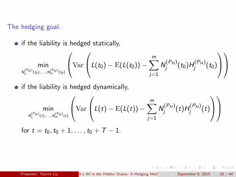
The hedging goal:
if the liability is hedged statically,
minN
(PH )1 (t0),...,N
(PH )m (t0)
Var
L(t0)− E(L(t0))−m∑j=1
N(PH)j (t0)H
(PH)j (t0)
if the liability is hedged dynamically,
minN
(PH )1 (t),...,N
(PH )m (t)
Var
L(t)− E(L(t))−m∑j=1
N(PH)j (t)H
(PH)j (t)
for t = t0, t0 + 1, . . . , t0 + T − 1.
Presenter: Yanxin Liu It’s All in the Hidden States: A Hedging Method with an Explicit Measure of Population Basis RiskSeptember 9, 2015 18 / 44
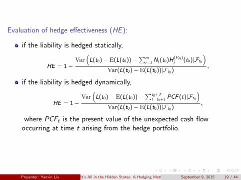
Evaluation of hedge effectiveness (HE ):
if the liability is hedged statically,
HE = 1−Var
(L(t0)− E(L(t0))−
∑mj=1 Nj(t0)H
(PH )j (t0)|Ft0
)Var(L(t0)− E(L(t0))|Ft0 )
,
if the liability is hedged dynamically,
HE = 1−Var
(L(t0)− E(L(t0))−
∑t0+Tt=t0+1 PCF (t)|Ft0
)Var(L(t0)− E(L(t0))|Ft0 )
,
where PCFt is the present value of the unexpected cash flowoccurring at time t arising from the hedge portfolio.
Presenter: Yanxin Liu It’s All in the Hidden States: A Hedging Method with an Explicit Measure of Population Basis RiskSeptember 9, 2015 19 / 44
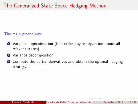
The Generalized State Space Hedging Method
The main procedures:
1 Variance approximation (first-order Taylor expansion about allrelevant states).
2 Variance decomposition.
3 Compute the partial derivatives and obtain the optimal hedgingstrategy.
Presenter: Yanxin Liu It’s All in the Hidden States: A Hedging Method with an Explicit Measure of Population Basis RiskSeptember 9, 2015 20 / 44
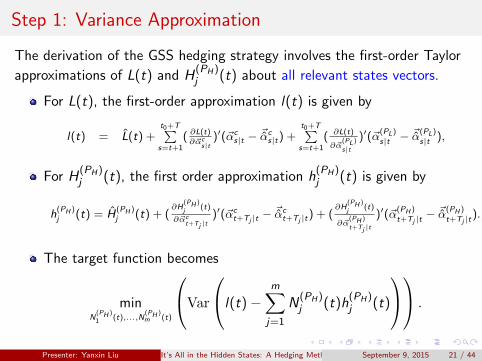
Step 1: Variance Approximation
The derivation of the GSS hedging strategy involves the first-order Taylor
approximations of L(t) and H(PH)j (t) about all relevant states vectors.
For L(t), the first-order approximation l(t) is given by
l(t) = L(t) +t0+T∑s=t+1
( ∂L(t)∂~αc
s|t)′(~αc
s|t − ~αcs|t) +
t0+T∑s=t+1
( ∂L(t)
∂~α(PL)
s|t
)′(~α(PL)s|t − ~α
(PL)s|t ),
For H(PH)j (t), the first order approximation h
(PH)j (t) is given by
h(PH )j (t) = H
(PH )j (t) + (
∂H(PH )
j (t)
∂~αct+Tj |t
)′(~αct+Tj |t − ~α
ct+Tj |t) + (
∂H(PH )
j (t)
∂~α(PH )
t+Tj |t
)′(~α(PH )t+Tj |t
− ~α(PH )t+Tj |t
).
The target function becomes
minN
(PH )1 (t),...,N
(PH )m (t)
Var
l(t)−m∑j=1
N(PH)j (t)h
(PH)j (t)
.
Presenter: Yanxin Liu It’s All in the Hidden States: A Hedging Method with an Explicit Measure of Population Basis RiskSeptember 9, 2015 21 / 44
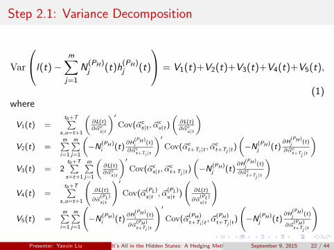
Step 2.1: Variance Decomposition
Var
l(t)−m∑j=1
N(PH)j (t)h
(PH)j (t)
= V1(t)+V2(t)+V3(t)+V4(t)+V5(t),
(1)where
V1(t) =t0+T∑
s,u=t+1
(∂L(t)∂~αc
s|t
)′Cov(~αc
s|t , ~αcu|t)
(∂L(t)∂~αc
u|t
)V2(t) =
m∑i=1
m∑j=1
(−N(PH )
i (t)∂H
(PH )
i (t)
∂~αct+Ti |t
)′Cov(~αc
t+Ti |t , ~αct+Tj |t)
(−N(PH )
j (t)∂H
(PH )
j (t)
∂~αct+Tj |t
)V3(t) = 2
t0+T∑s=t+1
m∑j=1
(∂L(t)∂~αc
s|t
)′Cov(~αc
s|t , ~αct+Tj |t)
(−N(PH )
j (t)∂H
(PH )
j (t)
∂~αct+Tj |t
)V4(t) =
t0+T∑s,u=t+1
(∂L(t)
∂~α(PL)
s|t
)′Cov(~α
(PL)s|t , ~α
(PL)u|t )
(∂L(t)
∂~α(PL)
u|t
)
V5(t) =m∑i=1
m∑j=1
(−N(PH )
i (t)∂H
(PH )
i (t)
∂~α(PH )
t+Ti |t
)′Cov(~α
(PH )t+Ti |t
, ~α(PH )t+Tj |t
)
(−N(PH )
j (t)∂H
(PH )
j (t)
∂~α(PH )
t+Tj |t
)
Presenter: Yanxin Liu It’s All in the Hidden States: A Hedging Method with an Explicit Measure of Population Basis RiskSeptember 9, 2015 22 / 44
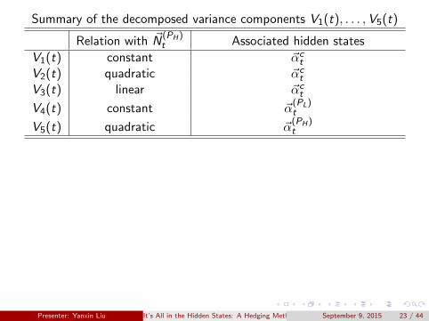
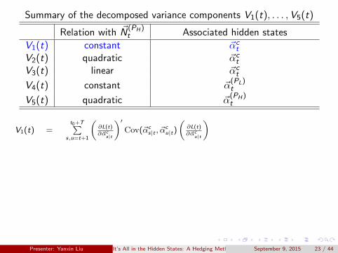
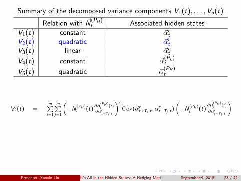
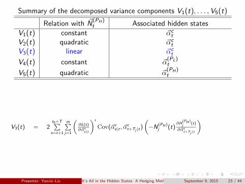
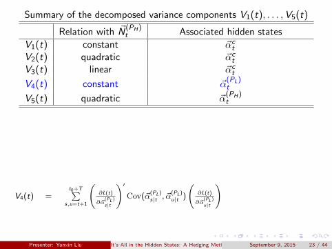
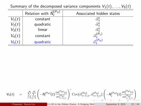
Summary of the decomposed variance components V1(t), . . . ,V5(t)
Relation with ~N(PH)t Associated hidden states
V1(t) constant ~αct
V2(t) quadratic ~αct
V3(t) linear ~αct
V4(t) constant ~α(PL)t
V5(t) quadratic ~α(PH)t
V1(t) =t0+T∑
s,u=t+1
(∂L(t)∂~αc
s|t
)′Cov(~αc
s|t , ~αcu|t)
(∂L(t)∂~αc
u|t
)V2(t) =
m∑i=1
m∑j=1
(−N(PH )
i (t)∂H
(PH )
i (t)
∂~αct+Ti |t
)′Cov(~αc
t+Ti |t , ~αct+Tj |t)
(−N(PH )
j (t)∂H
(PH )
j (t)
∂~αct+Tj |t
)V3(t) = 2
t0+T∑s=t+1
m∑j=1
(∂L(t)∂~αc
s|t
)′Cov(~αc
s|t , ~αct+Tj |t)
(−N(PH )
j (t)∂H
(PH )
j (t)
∂~αct+Tj |t
)V4(t) =
t0+T∑s,u=t+1
(∂L(t)
∂~α(PL)
s|t
)′Cov(~α
(PL)s|t , ~α
(PL)u|t )
(∂L(t)
∂~α(PL)
u|t
)
V5(t) =m∑i=1
m∑j=1
(−N(PH )
i (t)∂H
(PH )
i (t)
∂~α(PH )
t+Ti |t
)′Cov(~α
(PH )t+Ti |t
, ~α(PH )t+Tj |t
)
(−N(PH )
j (t)∂H
(PH )
j (t)
∂~α(PH )
t+Tj |t
)
Presenter: Yanxin Liu It’s All in the Hidden States: A Hedging Method with an Explicit Measure of Population Basis RiskSeptember 9, 2015 23 / 44
Summary of the decomposed variance components V1(t), . . . ,V5(t)
Relation with ~N(PH)t Associated hidden states
V1(t) constant ~αct
V2(t) quadratic ~αct
V3(t) linear ~αct
V4(t) constant ~α(PL)t
V5(t) quadratic ~α(PH)t
V1(t) =t0+T∑
s,u=t+1
(∂L(t)∂~αc
s|t
)′Cov(~αc
s|t , ~αcu|t)
(∂L(t)∂~αc
u|t
)
V2(t) =m∑i=1
m∑j=1
(−N(PH )
i (t)∂H
(PH )
i (t)
∂~αct+Ti |t
)′Cov(~αc
t+Ti |t , ~αct+Tj |t)
(−N(PH )
j (t)∂H
(PH )
j (t)
∂~αct+Tj |t
)
V3(t) = 2t0+T∑s=t+1
m∑j=1
(∂L(t)∂~αc
s|t
)′Cov(~αc
s|t , ~αct+Tj |t)
(−N(PH )
j (t)∂H
(PH )
j (t)
∂~αct+Tj |t
)V4(t) =
t0+T∑s,u=t+1
(∂L(t)
∂~α(PL)
s|t
)′Cov(~α
(PL)s|t , ~α
(PL)u|t )
(∂L(t)
∂~α(PL)
u|t
)
V5(t) =m∑i=1
m∑j=1
(−N(PH )
i (t)∂H
(PH )
i (t)
∂~α(PH )
t+Ti |t
)′Cov(~α
(PH )t+Ti |t
, ~α(PH )t+Tj |t
)
(−N(PH )
j (t)∂H
(PH )
j (t)
∂~α(PH )
t+Tj |t
)
Presenter: Yanxin Liu It’s All in the Hidden States: A Hedging Method with an Explicit Measure of Population Basis RiskSeptember 9, 2015 23 / 44
Summary of the decomposed variance components V1(t), . . . ,V5(t)
Relation with ~N(PH)t Associated hidden states
V1(t) constant ~αct
V2(t) quadratic ~αct
V3(t) linear ~αct
V4(t) constant ~α(PL)t
V5(t) quadratic ~α(PH)t
V1(t) =t0+T∑
s,u=t+1
(∂L(t)∂~αc
s|t
)′Cov(~αc
s|t , ~αcu|t)
(∂L(t)∂~αc
u|t
)V2(t) =
m∑i=1
m∑j=1
(−N(PH )
i (t)∂H
(PH )
i (t)
∂~αct+Ti |t
)′Cov(~αc
t+Ti |t , ~αct+Tj |t)
(−N(PH )
j (t)∂H
(PH )
j (t)
∂~αct+Tj |t
)
V3(t) = 2t0+T∑s=t+1
m∑j=1
(∂L(t)∂~αc
s|t
)′Cov(~αc
s|t , ~αct+Tj |t)
(−N(PH )
j (t)∂H
(PH )
j (t)
∂~αct+Tj |t
)
V4(t) =t0+T∑
s,u=t+1
(∂L(t)
∂~α(PL)
s|t
)′Cov(~α
(PL)s|t , ~α
(PL)u|t )
(∂L(t)
∂~α(PL)
u|t
)
V5(t) =m∑i=1
m∑j=1
(−N(PH )
i (t)∂H
(PH )
i (t)
∂~α(PH )
t+Ti |t
)′Cov(~α
(PH )t+Ti |t
, ~α(PH )t+Tj |t
)
(−N(PH )
j (t)∂H
(PH )
j (t)
∂~α(PH )
t+Tj |t
)
Presenter: Yanxin Liu It’s All in the Hidden States: A Hedging Method with an Explicit Measure of Population Basis RiskSeptember 9, 2015 23 / 44
Summary of the decomposed variance components V1(t), . . . ,V5(t)
Relation with ~N(PH)t Associated hidden states
V1(t) constant ~αct
V2(t) quadratic ~αct
V3(t) linear ~αct
V4(t) constant ~α(PL)t
V5(t) quadratic ~α(PH)t
V1(t) =t0+T∑
s,u=t+1
(∂L(t)∂~αc
s|t
)′Cov(~αc
s|t , ~αcu|t)
(∂L(t)∂~αc
u|t
)V2(t) =
m∑i=1
m∑j=1
(−N(PH )
i (t)∂H
(PH )
i (t)
∂~αct+Ti |t
)′Cov(~αc
t+Ti |t , ~αct+Tj |t)
(−N(PH )
j (t)∂H
(PH )
j (t)
∂~αct+Tj |t
)V3(t) = 2
t0+T∑s=t+1
m∑j=1
(∂L(t)∂~αc
s|t
)′Cov(~αc
s|t , ~αct+Tj |t)
(−N(PH )
j (t)∂H
(PH )
j (t)
∂~αct+Tj |t
)
V4(t) =t0+T∑
s,u=t+1
(∂L(t)
∂~α(PL)
s|t
)′Cov(~α
(PL)s|t , ~α
(PL)u|t )
(∂L(t)
∂~α(PL)
u|t
)
V5(t) =m∑i=1
m∑j=1
(−N(PH )
i (t)∂H
(PH )
i (t)
∂~α(PH )
t+Ti |t
)′Cov(~α
(PH )t+Ti |t
, ~α(PH )t+Tj |t
)
(−N(PH )
j (t)∂H
(PH )
j (t)
∂~α(PH )
t+Tj |t
)
Presenter: Yanxin Liu It’s All in the Hidden States: A Hedging Method with an Explicit Measure of Population Basis RiskSeptember 9, 2015 23 / 44
Summary of the decomposed variance components V1(t), . . . ,V5(t)
Relation with ~N(PH)t Associated hidden states
V1(t) constant ~αct
V2(t) quadratic ~αct
V3(t) linear ~αct
V4(t) constant ~α(PL)t
V5(t) quadratic ~α(PH)t
V1(t) =t0+T∑
s,u=t+1
(∂L(t)∂~αc
s|t
)′Cov(~αc
s|t , ~αcu|t)
(∂L(t)∂~αc
u|t
)V2(t) =
m∑i=1
m∑j=1
(−N(PH )
i (t)∂H
(PH )
i (t)
∂~αct+Ti |t
)′Cov(~αc
t+Ti |t , ~αct+Tj |t)
(−N(PH )
j (t)∂H
(PH )
j (t)
∂~αct+Tj |t
)V3(t) = 2
t0+T∑s=t+1
m∑j=1
(∂L(t)∂~αc
s|t
)′Cov(~αc
s|t , ~αct+Tj |t)
(−N(PH )
j (t)∂H
(PH )
j (t)
∂~αct+Tj |t
)V4(t) =
t0+T∑s,u=t+1
(∂L(t)
∂~α(PL)
s|t
)′Cov(~α
(PL)s|t , ~α
(PL)u|t )
(∂L(t)
∂~α(PL)
u|t
)
V5(t) =m∑i=1
m∑j=1
(−N(PH )
i (t)∂H
(PH )
i (t)
∂~α(PH )
t+Ti |t
)′Cov(~α
(PH )t+Ti |t
, ~α(PH )t+Tj |t
)
(−N(PH )
j (t)∂H
(PH )
j (t)
∂~α(PH )
t+Tj |t
)Presenter: Yanxin Liu It’s All in the Hidden States: A Hedging Method with an Explicit Measure of Population Basis RiskSeptember 9, 2015 23 / 44
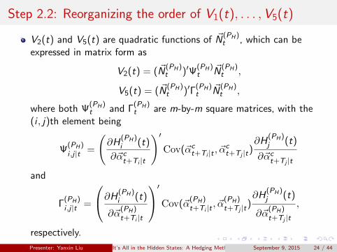
Step 2.2: Reorganizing the order of V1(t), . . . ,V5(t)
V2(t) and V5(t) are quadratic functions of ~N(PH)t , which can be
expressed in matrix form as
V2(t) = ( ~N(PH)t )′Ψ
(PH)t
~N(PH)t ,
V5(t) = ( ~N(PH)t )′Γ
(PH)t
~N(PH)t ,
where both Ψ(PH)t and Γ
(PH)t are m-by-m square matrices, with the
(i , j)th element being
Ψ(PH)i ,j |t =
(∂H
(PH)i (t)
∂~αct+Ti |t
)′Cov(~αc
t+Ti |t , ~αct+Tj |t)
∂H(PH)j (t)
∂~αct+Tj |t
and
Γ(PH)i ,j |t =
∂H(PH)i (t)
∂~α(PH)t+Ti |t
′Cov(~α(PH)t+Ti |t , ~α
(PH)t+Tj |t)
∂H(PH)j (t)
∂~α(PH)t+Tj |t
,
respectively.
Presenter: Yanxin Liu It’s All in the Hidden States: A Hedging Method with an Explicit Measure of Population Basis RiskSeptember 9, 2015 24 / 44
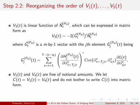
Step 2.2: Reorganizing the order of V1(t), . . . ,V5(t)
V3(t) is linear function of ~N(PH)t , which can be expressed in matrix
form asV3(t) = −2( ~G
(PH)t )′ ~N
(PH)t
where ~G(PH)t is a m-by-1 vector with the jth element G
(PH)j (t) being
G(PH)j (t) =
T−(t−t0)∑s=t+1
∂H(PH)j (t)
∂~αct+Tj |t
′Cov(~αct+Tj |t , ~α
cs|t)
∂L(t)
∂~αcs|t,
V1(t) and V4(t) are free of notional amounts. We letC (t) = V1(t) + V4(t) and do not bother to write C (t) into matrixform.
Presenter: Yanxin Liu It’s All in the Hidden States: A Hedging Method with an Explicit Measure of Population Basis RiskSeptember 9, 2015 25 / 44
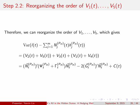
Step 2.2: Reorganizing the order of V1(t), . . . ,V5(t)
Therefore, we can reorganize the order of V1, . . . ,V5, which gives
Var(l(t)−∑m
j=1 N(PH)j (t)h
(PH)j (t))
= (V2(t) + V5(t)) + V3(t) + (V1(t) + V4(t))
= ( ~N(PH)t )′(Ψ
(PH)t + Γ
(PH)t ) ~N
(PH)t − 2( ~G
(PH)t )′ ~N
(PH)t + C (t)
Presenter: Yanxin Liu It’s All in the Hidden States: A Hedging Method with an Explicit Measure of Population Basis RiskSeptember 9, 2015 26 / 44
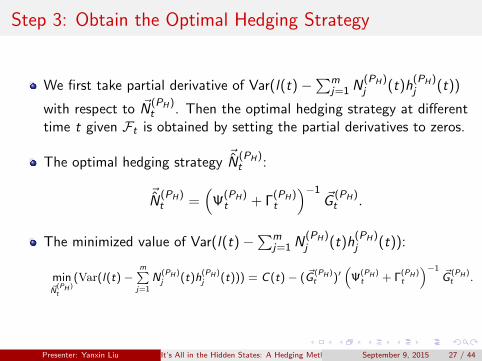
Step 3: Obtain the Optimal Hedging Strategy
We first take partial derivative of Var(l(t)−∑m
j=1 N(PH)j (t)h
(PH)j (t))
with respect to ~N(PH)t . Then the optimal hedging strategy at different
time t given Ft is obtained by setting the partial derivatives to zeros.
The optimal hedging strategy~N
(PH)t :
~N
(PH)t =
(Ψ
(PH)t + Γ
(PH)t
)−1~G
(PH)t .
The minimized value of Var(l(t)−∑m
j=1 N(PH)j (t)h
(PH)j (t)):
min~N
(PH )t
(Var(l(t)−m∑j=1
N(PH )j (t)h
(PH )j (t))) = C(t)− ( ~G
(PH )t )′
(Ψ
(PH )t + Γ
(PH )t
)−1~G
(PH )t .
Presenter: Yanxin Liu It’s All in the Hidden States: A Hedging Method with an Explicit Measure of Population Basis RiskSeptember 9, 2015 27 / 44
Outline
1 Introduction
2 The Applicable Mortality Models
3 The Generalized State Space Hedging Method
4 Analyzing Population Basis Risk
5 A Numerical Illustration
6 Conclusion
Presenter: Yanxin Liu It’s All in the Hidden States: A Hedging Method with an Explicit Measure of Population Basis RiskSeptember 9, 2015 28 / 44
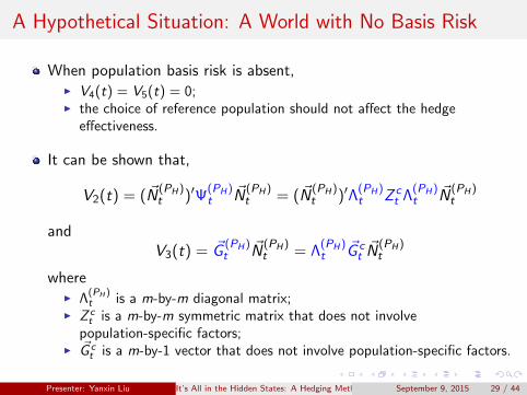
A Hypothetical Situation: A World with No Basis Risk
When population basis risk is absent,I V4(t) = V5(t) = 0;I the choice of reference population should not affect the hedge
effectiveness.
It can be shown that,
V2(t) = ( ~N(PH)t )′Ψ
(PH)t
~N(PH)t = ( ~N
(PH)t )′Λ
(PH)t Z c
t Λ(PH)t
~N(PH)t
andV3(t) = ~G
(PH)t
~N(PH)t = Λ
(PH)t
~G ct~N
(PH)t
whereI Λ
(PH )t is a m-by-m diagonal matrix;
I Z ct is a m-by-m symmetric matrix that does not involve
population-specific factors;I ~G c
t is a m-by-1 vector that does not involve population-specific factors.
Presenter: Yanxin Liu It’s All in the Hidden States: A Hedging Method with an Explicit Measure of Population Basis RiskSeptember 9, 2015 29 / 44
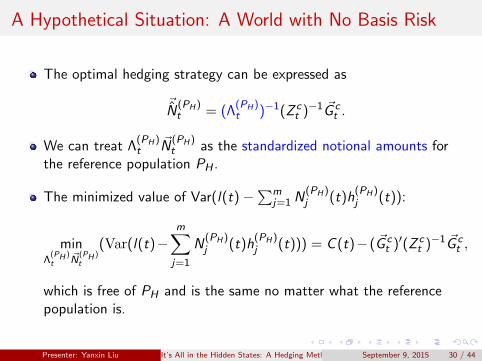
A Hypothetical Situation: A World with No Basis Risk
The optimal hedging strategy can be expressed as
~N
(PH)t = (Λ
(PH)t )−1(Z c
t )−1 ~G ct .
We can treat Λ(PH)t
~N(PH)t as the standardized notional amounts for
the reference population PH .
The minimized value of Var(l(t)−∑m
j=1 N(PH)j (t)h
(PH)j (t)):
minΛ
(PH )t
~N(PH )t
(Var(l(t)−m∑j=1
N(PH)j (t)h
(PH)j (t))) = C (t)− ( ~G c
t )′(Z ct )−1 ~G c
t ,
which is free of PH and is the same no matter what the referencepopulation is.
Presenter: Yanxin Liu It’s All in the Hidden States: A Hedging Method with an Explicit Measure of Population Basis RiskSeptember 9, 2015 30 / 44
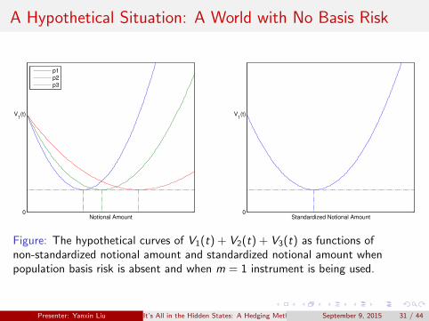
A Hypothetical Situation: A World with No Basis Risk
0
V1(t)
Notional Amount
p1
p2
p3
0
V1(t)
Standardized Notional Amount
Figure: The hypothetical curves of V1(t) + V2(t) + V3(t) as functions ofnon-standardized notional amount and standardized notional amount whenpopulation basis risk is absent and when m = 1 instrument is being used.
Presenter: Yanxin Liu It’s All in the Hidden States: A Hedging Method with an Explicit Measure of Population Basis RiskSeptember 9, 2015 31 / 44
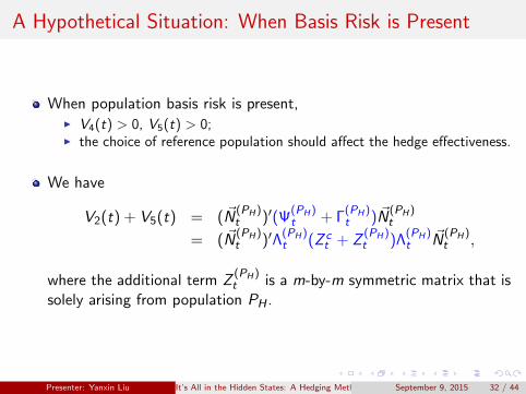
A Hypothetical Situation: When Basis Risk is Present
When population basis risk is present,I V4(t) > 0, V5(t) > 0;I the choice of reference population should affect the hedge effectiveness.
We have
V2(t) + V5(t) = ( ~N(PH)t )′(Ψ
(PH)t + Γ
(PH)t ) ~N
(PH)t
= ( ~N(PH)t )′Λ
(PH)t (Z c
t + Z(PH)t )Λ
(PH)t
~N(PH)t ,
where the additional term Z(PH)t is a m-by-m symmetric matrix that is
solely arising from population PH .
Presenter: Yanxin Liu It’s All in the Hidden States: A Hedging Method with an Explicit Measure of Population Basis RiskSeptember 9, 2015 32 / 44
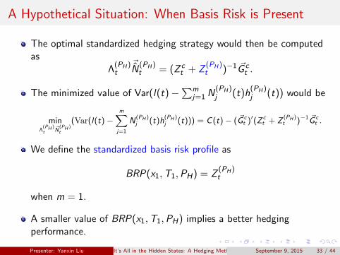
A Hypothetical Situation: When Basis Risk is Present
The optimal standardized hedging strategy would then be computedas
Λ(PH)t
~N
(PH)t = (Z c
t + Z(PH)t )−1 ~G c
t .
The minimized value of Var(l(t)−∑m
j=1 N(PH)j (t)h
(PH)j (t)) would be
minΛ
(PH )t
~N(PH )t
(Var(l(t)−m∑j=1
N(PH )j (t)h
(PH )j (t))) = C(t)− ( ~G c
t )′(Z ct + Z
(PH )t )−1 ~G c
t .
We define the standardized basis risk profile as
BRP(x1,T1,PH) = Z(PH)t
when m = 1.
A smaller value of BRP(x1,T1,PH) implies a better hedgingperformance.
Presenter: Yanxin Liu It’s All in the Hidden States: A Hedging Method with an Explicit Measure of Population Basis RiskSeptember 9, 2015 33 / 44
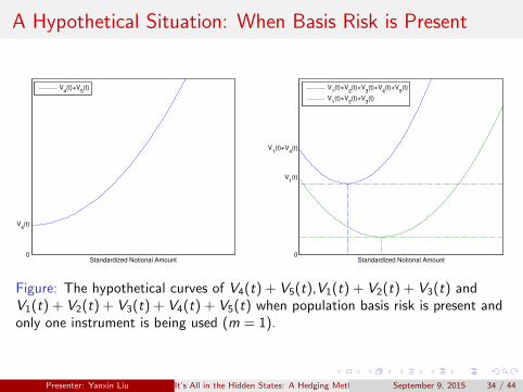
A Hypothetical Situation: When Basis Risk is Present
0
V4(t)
Standardized Notional Amount
V4(t)+V
5(t)
0
V1(t)
V1(t)+V
4(t)
Standardized Notional Amount
V1(t)+V
2(t)+V
3(t)+V
4(t)+V
5(t)
V1(t)+V
2(t)+V
3(t)
Figure: The hypothetical curves of V4(t) + V5(t),V1(t) + V2(t) + V3(t) andV1(t) + V2(t) + V3(t) + V4(t) + V5(t) when population basis risk is present andonly one instrument is being used (m = 1).
Presenter: Yanxin Liu It’s All in the Hidden States: A Hedging Method with an Explicit Measure of Population Basis RiskSeptember 9, 2015 34 / 44
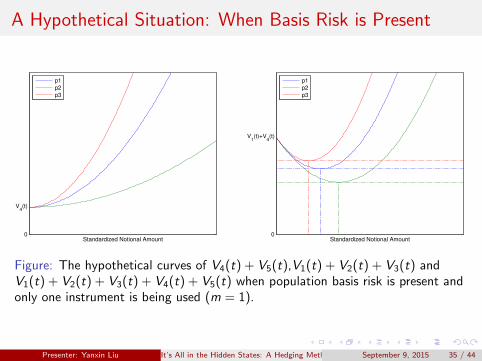
A Hypothetical Situation: When Basis Risk is Present
0
V4(t)
Standardized Notional Amount
p1
p2
p3
0
V1(t)+V
4(t)
Standardized Notional Amount
p1
p2
p3
Figure: The hypothetical curves of V4(t) + V5(t),V1(t) + V2(t) + V3(t) andV1(t) + V2(t) + V3(t) + V4(t) + V5(t) when population basis risk is present andonly one instrument is being used (m = 1).
Presenter: Yanxin Liu It’s All in the Hidden States: A Hedging Method with an Explicit Measure of Population Basis RiskSeptember 9, 2015 35 / 44

Outline
1 Introduction
2 The Applicable Mortality Models
3 The Generalized State Space Hedging Method
4 Analyzing Population Basis Risk
5 A Numerical Illustration
6 Conclusion
Presenter: Yanxin Liu It’s All in the Hidden States: A Hedging Method with an Explicit Measure of Population Basis RiskSeptember 9, 2015 36 / 44
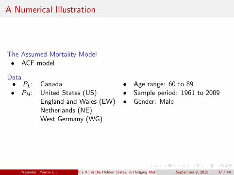
A Numerical Illustration
The Assumed Mortality Model• ACF model
Data• PL: Canada • Age range: 60 to 89• PH : United States (US) • Sample period: 1961 to 2009
England and Wales (EW) • Gender: MaleNetherlands (NE)West Germany (WG)
Presenter: Yanxin Liu It’s All in the Hidden States: A Hedging Method with an Explicit Measure of Population Basis RiskSeptember 9, 2015 37 / 44
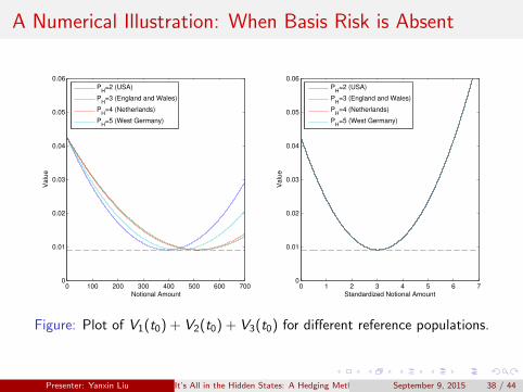
A Numerical Illustration: When Basis Risk is Absent
0 100 200 300 400 500 600 7000
0.01
0.02
0.03
0.04
0.05
0.06
Notional Amount
Valu
e
PH
=2 (USA)
PH
=3 (England and Wales)
PH
=4 (Netherlands)
PH
=5 (West Germany)
0 1 2 3 4 5 6 70
0.01
0.02
0.03
0.04
0.05
0.06
Standardized Notional Amount
Valu
e
PH
=2 (USA)
PH
=3 (England and Wales)
PH
=4 (Netherlands)
PH
=5 (West Germany)
Figure: Plot of V1(t0) + V2(t0) + V3(t0) for different reference populations.
Presenter: Yanxin Liu It’s All in the Hidden States: A Hedging Method with an Explicit Measure of Population Basis RiskSeptember 9, 2015 38 / 44
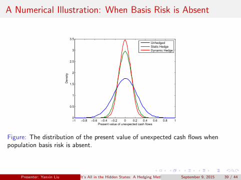
A Numerical Illustration: When Basis Risk is Absent
−1 −0.8 −0.6 −0.4 −0.2 0 0.2 0.4 0.6 0.8 10
0.5
1
1.5
2
2.5
3
3.5
Present value of unexpected cash flows
De
nsity
Unhedged
Static Hedge
Dynamic Hedge
Figure: The distribution of the present value of unexpected cash flows whenpopulation basis risk is absent.
Presenter: Yanxin Liu It’s All in the Hidden States: A Hedging Method with an Explicit Measure of Population Basis RiskSeptember 9, 2015 39 / 44
A Numerical Illustration: When Basis Risk is Present
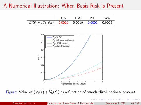
US EW NE WG
BRP(x1,T1,PH) 0.0020 0.0019 0.0003 0.0005
0 1 2 3 4 5 6 70
0.01
0.02
0.03
0.04
0.05
0.06
Standardized Notional Amount
Valu
e
PH
=2 (USA)
PH
=3 (England and Wales)
PH
=4 (Netherlands)
PH
=5 (West Germany)
Figure: Value of (V4(t) + V5(t)) as a function of standardized notional amount
Presenter: Yanxin Liu It’s All in the Hidden States: A Hedging Method with an Explicit Measure of Population Basis RiskSeptember 9, 2015 40 / 44

A Numerical Illustration: When Basis Risk is Present
US EW NE WG
HE (static) 0.5085 0.5143 0.7016 0.6761HE (dynamic) 0.6243 0.6279 0.8404 0.8213
−1 −0.8 −0.6 −0.4 −0.2 0 0.2 0.4 0.6 0.8 10
0.5
1
1.5
2
2.5
3
3.5
Present value of unexpected cash flows
Density
Unhedged
Static Hedge
Dynamic Hedge
(a) US
−1 −0.8 −0.6 −0.4 −0.2 0 0.2 0.4 0.6 0.8 10
0.5
1
1.5
2
2.5
3
3.5
Present value of unexpected cash flows
Density
Unhedged
Static Hedge
Dynamic Hedge
(b) EW
Figure: The distribution of the present value of unexpected cash flows whenpopulation basis risk is present.
Presenter: Yanxin Liu It’s All in the Hidden States: A Hedging Method with an Explicit Measure of Population Basis RiskSeptember 9, 2015 41 / 44
A Numerical Illustration: When Basis Risk is Present
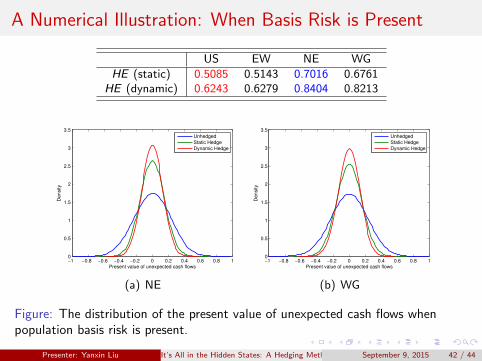
US EW NE WG
HE (static) 0.5085 0.5143 0.7016 0.6761HE (dynamic) 0.6243 0.6279 0.8404 0.8213
−1 −0.8 −0.6 −0.4 −0.2 0 0.2 0.4 0.6 0.8 10
0.5
1
1.5
2
2.5
3
3.5
Present value of unexpected cash flows
Density
Unhedged
Static Hedge
Dynamic Hedge
(a) NE
−1 −0.8 −0.6 −0.4 −0.2 0 0.2 0.4 0.6 0.8 10
0.5
1
1.5
2
2.5
3
3.5
Present value of unexpected cash flows
Density
Unhedged
Static Hedge
Dynamic Hedge
(b) WG
Figure: The distribution of the present value of unexpected cash flows whenpopulation basis risk is present.
Presenter: Yanxin Liu It’s All in the Hidden States: A Hedging Method with an Explicit Measure of Population Basis RiskSeptember 9, 2015 42 / 44

Outline
1 Introduction
2 The Applicable Mortality Models
3 The Generalized State Space Hedging Method
4 Analyzing Population Basis Risk
5 A Numerical Illustration
6 Conclusion
Presenter: Yanxin Liu It’s All in the Hidden States: A Hedging Method with an Explicit Measure of Population Basis RiskSeptember 9, 2015 43 / 44
Concluding Remarks
The generalized state space hedging method is proposed for use whenthe populations associated with the hedging instruments and theliability being hedged are different.
The GSS hedging method can also be applied to mortality modelswith cohort effect, as long as the model can be written in state spaceform.
A quantity called standardized basis risk profile BRP(x1,T1,PH) hasbeen developed.
A numerical illustration has been provided to demonstrate the use ofBRP(x1,T1,PH).
Presenter: Yanxin Liu It’s All in the Hidden States: A Hedging Method with an Explicit Measure of Population Basis RiskSeptember 9, 2015 44 / 44