It’s All in the Hidden States: A Hedging Method

with an Explicit Measure of Population Basis Risk

Yanxin Liu∗ and Johnny Siu-Hang Li†

November 2, 2015

Abstract

In this paper, we propose the generalized state-space hedging method for use when the populations

associated with the hedging instruments and the liability being hedged are different. In this method,

the hedging strategy is derived by first reformulating the assumed multi-population stochastic mortality

model in a state-space representation, and then considering the sensitivities of the hedge portfolio and

the liability being hedged to all relevant hidden states. Inter alia, this method allows us to decompose

the underlying longevity risk into components arising solely from the hidden states that are shared

by all populations and components stemming exclusively from the hidden states that are population-

specific. The latter components collectively represent an explicit measure of the population basis risk

involved. Through this measure, we can infer that a portion of population basis risk depends on how

the longevity hedge is constructed while another portion exists no matter what the notional amounts

of the hedging instruments are. We present the proposed hedging method in both static and dynamic

settings.

Key words: Coherent mortality forecasting; Index-based longevity hedges; Multi-population mortality

models; q-forwards; State-space models

1 Introduction

Longevity risk refers to the adverse financial consequences that arise when individuals live longer than

expected. The risk affects sponsors of defined-benefit pension plans heavily, as the longer people live the

larger the pension liabilities are. The threat of longevity risk to pension plan sponsors has become even

more apparent in recent years, due in part to the low-yield environment after the financial crisis of 2007-08

and in part to the more conservative mortality improvement scales that are recently introduced by the

actuarial profession (Canadian Institute of Actuaries, 2014; Continuous Mortality Investigation Bureau,

2009a,b; Society of Actuaries, 2014). In response to the problem, pension longevity risk transfers started

to emerge in early 2000s, providing opportunities for pension plan sponsors to transfer longevity risk to

entities that are in a better position to run the risk.

∗Yanxin Liu is a Ph.D. candidate in the Department of Statistics and Actuarial Science at the University of Waterloo,Canada. Email: y473liu@uwaterloo.ca.†Johnny Siu-Hang Li holds the Fairfax Chair in Risk Management in the Department of Statistics and Actuarial Science

at the University of Waterloo, Canada. Email: shli@uwaterloo.ca.

1

The majority of the pension longevity risk transfers executed to date are insurance-based buy-outs,

buy-ins and bespoke longevity swaps. However, the insurance industry is unable to take an unlimited

amount of longevity risk, because of the systematic nature of risk and the capital requirements imposed

by Solvency II or its equivalent. The analyses of Graziani (2014) and Michaelson and Mulholland (2014)

concluded that the global insurance industry can only absorb a fraction of the longevity risk exposure from

defined-benefit pension plans worldwide. Consequently, there is a need to search for additional participants

who are willing to accept the risk. One possible candidate is capital market investors, who are possibly

interested in the longevity asset class because of the risk premium and diversification benefit it offers.

Capital market investors demand liquidity and are likely to be discouraged by the information asym-

metry arising from the fact that pension plan sponsors know better about the mortality experience of

the individuals associated with their portfolios. To attract their participation, longevity risk needs to be

packaged as standardized index-based mortality derivatives. Several successful attempts of standardization

have been made. The first took place in January 2008 when J.P. Morgan executed a mortality (q-) forward

contract with Lucida, a monoline insurer in the UK.1 Other examples include the £70 million 10-year

q-forward that J.P. Morgan transacted with the Pall (UK) Pension fund in January 20112 and the e12

billion index-based longevity swap executed between Deutsche Bank and Aegon in February 2012.3 More

recently, Deutsche Bank launched in November 2013 the Longevity Experience Option (LEO), which is

structured as an out-of-the-money call option spread on 10-year forward survival rates and has a maturity

of 10 years. The first LEO was reportedly traded in January 2014.4 At present, tradable longevity indexes

include the LifeMetrics Index provided by the Life and Longevity Markets Association (LLMA) and the

Xpect Club Vita Index provided by Deutsche Borse.

Nevertheless, the market for index-based mortality derivatives is still quite far from being large and

liquid, and is facing several challenges. On the supply side, a few major investment banks, namely Credit

Suisse, Normura and UBS, left the market for longevity risk transfers in 2012 for regulatory reasons (Tan et

al., 2015). On the demand side, as noted by Blake et al. (2013), the major challenge is “the continuing re-

sistance of pension plan trustees and their advisors, as well as insurers and reinsurers, to imperfect hedging

solutions of the capital markets.” Longevity hedges developed from index-based mortality derivatives are

imperfect, because there exists population basis risk which arises from the difference in mortality improve-

ments between the populations associated with the hedger and the index used for hedging purposes. The

challenge on the demand side calls for research to address the following questions: (1) How to quantify the

exposure to population basis risk in an index-based longevity hedge? (2) How to optimize an index-based

longevity hedge when population basis risk is taken into account? (3) How risk management decisions, for

example, selection of the most appropriate reference population, can be made in a world where population

basis risk exists?

Although a large number of multi-population stochastic mortality models have been proposed,5 only a

few attempts have been made to investigate how such models can be used to generate meaningful measures

of population basis risk. Previous studies on measuring population basis risk, including the work of Cairns

et al. (2014), Li and Hardy (2011) and Ngai and Sherris (2011), typically follow the framework set out by

Coughlan et al. (2011). The framework encompasses the following two steps: (i) calibrate the portfolio of

1Source: http://www.efinancialnews.com/story/2008-02-19/lucida-guards-against-longevity2Source: http://www.pensionsworld.co.uk/article/first-longevity-hedge-non-retired-pension-plan-members3Source: https://www.db.com/medien/en/content/3862 4047.htm4Source: http://www.trading-risk.com/deutsche-bank-longevity-option-platform-closes-debut-deal5See, for example, D’Amato et al. (2014), Li and Lee (2005), Cairns et al. (2011), Dowd et al. (2011a), Jarner and Kryger

(2011), Ahmadi and Li (2014), Hatzopoulos and Haberman (2013), Hunt and Blake (2015), Yang and Wang (2013), and Zhouet al. (2013, 2014).

2

hedging instruments; (ii) calculate the amount of risk that the hedge can reduce on the basis of a large

number of scenarios simulated from the assumed stochastic mortality model. The two steps are performed

under the assumptions that population basis risk is absent and present, and the difference between the

results under the two assumptions represents the population basis risk that the hedger is subject to. Because

this approach depends on a calibrated longevity hedge, it does not readily indicate how population basis

risk varies as the composition of the hedge portfolio changes. In addition, the heavy reliance on simulations

makes this approach rather computationally demanding.

Strategies for optimizing an index-based longevity hedge have been developed by researchers including

Cairns (2011, 2013), Cairns et al. (2006b, 2014), Coughlan et al. (2011), Dahl (2004), Dahl and Møller

(2006), Dahl et al. (2008), Dowd et al. (2011b), Li and Hardy (2011), Li and Luo (2012), Luciano et

al. (2012), and Zhou and Li (2014). Generally speaking, the hedging strategies were derived by matching

the sensitivities of the liability being hedged and the portfolio of hedging instruments with respect to

changes in the underlying mortality rates. Most of the existing longevity hedging strategies are subject

to one significant limitation: they were developed under the ideal assumption that population basis risk

does not exist. Although Dowd et al. (2011b), Li and Hardy (2011), Li and Luo (2012) and Zhou and

Li (2014) studied how hedging strategies may be adjusted when population basis risk is present, their

adjustment formulas are derived on the basis of specific multi-population mortality models. For example,

the adjustment formula proposed by Li and Luo (2012) depends heavily on the augmented common factor

model (Li and Lee, 2005) and is consequently incompatible with other model assumptions. A more general

framework for hedging in the presence of population basis risk is yet to be sought.

The objectives of this paper are threefold. The first objective is to develop a hedging strategy that

explicitly incorporates population basis risk. This objective is achieved by extending the generalized state-

space hedging method proposed by Liu and Li (2014) to incorporate the random deviation between the

mortality improvements of the populations associated with the hedging instruments and the liability being

hedged. We choose to use the generalized state-space hedging method as a starting point, because, as

Liu and Li (2014) explained, the method ameliorates the problems of sub-optimality and singularity that

are found in the delta-nuga hedging method of Cairns (2013) and imposes less stringent requirements

on the number of hedging instruments used. In our proposed method, the hedging strategy is derived

by first reformulating the assumed multi-population stochastic mortality model in a state-space form,

and then considering the sensitivities of the hedge portfolio and the liability being hedged to all relevant

hidden states. Our proposed method is rather general in the sense that it can be applied to any coherent

multi-population mortality model, provided that the model can be expressed in a state-space form. We

demonstrate in the next section that the applicable models include the multi-population versions of the

Lee-Carter and Cairns-Blake-Dowd models (Lee and Carter, 1992; Cairns et al., 2006). The proposed

hedging method is presented in both static and dynamic settings, and the benefit of dynamically adjusting

a longevity hedge is studied.

The second objective is to develop an efficient method for quantifying the population basis risk in a

longevity hedge. To this end, we introduce a method to analytically approximate the variance of the time-t

values of an annuity portfolio, with or without a longevity hedge. The method enables us to estimate hedge

effectiveness (defined as the reduction in variance) without using simulation. As such, we can readily gauge

how much hedge effectiveness is eroded by population basis risk under different hedge portfolio composi-

tions. We also show that the approximated variance of a hedged annuity portfolio can be decomposed into

components arising solely from the hidden states that are shared by all populations and components stem-

ming exclusively from the hidden states that are population-specific. The latter components collectively

3

represent an explicit measure of the population basis risk involved in the longevity hedge. Furthermore,

from the mathematical formulation of this measure, we can infer that a portion of population basis risk

depends on how the longevity hedge is constructed while another portion exists no matter what the no-

tional amounts of the hedging instruments are. The intuitions behind the decomposition of variance and

the measure of population basis risk are illustrated extensively by graphical means throughout the paper.

The final objective is to develop a metric for assessing the relative levels of population basis risk that

different hedging instruments may lead to. We propose a metric called ‘standardized basis risk profile’, with

which we can compare the resulting population basis risk when q-forwards with different reference ages,

maturities and reference populations are used. The standardized basis risk profile is of practical importance.

For instance, let us suppose that a pension plan sponsor in Canada is contemplating hedging its longevity

risk exposure with q-forwards that are linked to a LifeMetrics Index. At present, the LifeMetrics Index

is available in England and Wales, the US, Germany and the Netherlands, but not in Canada. The

standardized basis risk profile can aid this pension plan sponsor in selecting one out of the four available

reference populations. While the methods proposed previously by Cairns (2011, 2013), Cairns et al. (2014),

Coughlan et al. (2011) and Li and Hardy (2011) may also be used for the purpose of reference population

selection, they generally require significant computational effort. In contrast, the standardized basis risk

profile can be computed analytically, and the comparison between different standardized basis risk profiles

can be made without calibrating the associated hedges in advance.

The remainder of this paper is organized as follows. Section 2 describes the collection of multi-population

mortality models to which the proposed hedging strategy can be applied. Section 3 presents the proposed

hedging strategy and the analytical decomposition of the portfolio variance. Section 4 explains how the

decomposition of variance can be utilized to measure population basis risk and defines the standardized

basis risk profile. Section 5 illustrates the proposed methodologies using real mortality data from various

national populations. Finally, Section 6 concludes the paper.

2 The Applicable Multi-Population Mortality Models

The proposed hedging method is quite general in the sense that it can be applied to any coherent multi-

population mortality model, provided that the model can be expressed in a state-space form. In what

follows, we first present the general state-space representation, and then illustrate how existing coherent

multi-population mortality models can be formulated in state-space forms.

2.1 The General State-Space Representation

Generally speaking, a state-space representation is composed of two components: (1) an observation equa-

tion that describes the connection between the observations and hidden states, and (2) a transition equation

that captures the evolution of the hidden states through a Markov process. Let ~yt and ~αt be the vectors

of observations and hidden states at time t, respectively. The observation equation is defined as

~yt = ~A+B~αt + ~εt, (2.1)

where ~A is a vector of constant terms, B is the design matrix which specifies the linear relationship between

the observations ~yt and the hidden states ~αt, and ~εt is a vector of observation errors that has a zero mean

4

and a constant covariance matrix R. The transition equation is defined as

~αt = ~U +D~αt−1 + ~ηt, (2.2)

where ~U represents the vector of drifts, D is a matrix which specifies the relationship between ~αt and ~αt−1,

and ~ηt is a vector of innovations that has a zero mean and a constant covariance matrix Q.

In the context of multi-population mortality modeling, the observation vector ~yt contains the time-t

values of the (transformed) age-specific death rates or probabilities for all of the populations being modeled.

Suppose that the number of populations being modeled is np. We can express ~yt as ((~y(1)t )′, . . . , (~y

(np)t )′)′,

with ~y(p)t , p = 1, . . . , np, representing the vector of (transformed) age-specific death rates or probabilities

for population p. If the age range under consideration is [xa, xb], then ~y(p)t = (y

(p)xa,t, y

(p)xa+1,t, . . . , y

(p)xb,t

)′.

A typical multi-population mortality model contains several stochastic components, some of which apply

to all of the populations being modeled while the other of which are population-specific. Accordingly, we

can express the state vector as ~αt = ((~αct)′, (~α

(1)t )′, . . . , (~α

(np)t )′)′, where ~αct encompasses the hidden states

that are shared by all of the populations being modeled and ~α(p)t , p = 1, . . . , np, consists of the hidden

states that belong exclusively to population p. In the sequel, we call ~αct the vector of ‘common states’ and

~α(p)t a vector of ‘population-specific states’.

We require the multi-population mortality model to be ‘coherent’. A coherent multi-population mor-

tality model is constructed in such a way to avoid a long-term divergence between projected mortality

trajectories of different populations, an outcome that is deemed to be biologically unreasonable. The con-

cept of coherent multi-population mortality forecasting was first proposed by Li and Lee (2005), who also

specified the following sufficient conditions for coherence: (i) all of the populations being modeled have

the same age-response to the common stochastic factors; (ii) the population-specific stochastic factors are

mean-reverting.

When formulated in a state-space representation, condition (i) means that the coefficients of the common

states for all of the populations being modeled are the same. Equivalently speaking, the design matrix B

should satisfy the following structure:

B =

Bc B(1) 0 · · · 0

Bc 0 B(2) · · · 0...

......

. . ....

Bc 0 0 · · · B(np)

, (2.3)

where

Bc =

(~bcxa

)′

...

(~bcxb)′

and B(p) =

(~b

(p)xa )′

...

(~b(p)xb )′

for p = 1, . . . , np. In the above, ~bcx is the vector of the coefficients of ~αct (the common states) in y

(p)x,t and

does not depend on p; ~b(p)x , p = 1, . . . , np, is the vector of the coefficients of ~α

(p)t (the population-specific

states) in y(p)x,t and is allowed to depend on p. Condition (ii) means that ~α

(p)t , p = 1, . . . , np, follows a

certain autoregressive process.

In line with the structure of the state vector, we have ~ηt = ((~ηct )′, (~η

(1)t )′, . . . , (~η

(np)t )′)′, where ~ηct and

5

~η(p)t , p = 1, . . . , np, represent the innovation vectors in the processes for ~αct and ~α

(p)t , respectively. It is

assumed that ~ηct , ~η(1)t , ..., ~η

(np)t are mutually independent. Given this assumption, the covariance matrix

Q in the transition equation is a block diagonal matrix,

Q =

Qc 0 · · · 0

0 Q(1) 0...

. . ....

0 0 · · · Q(np)

, (2.4)

with Qc, Q(1), . . . , Q(np) representing the covariance matrices of ~ηct , ~η(1)t , . . . , ~η

(np)t , respectively. In the rest

of this section, we use two examples to illustrate how existing coherent multi-population mortality models

can be formulated using the general state-space representation.

2.2 The Augmented Common Factor Model

The first example is the Augmented Common Factor (ACF) model proposed by Li and Lee (2005). Let

m(p)x,t be population p’s central death rate at age x and in year t. The ACF model assumes that

ln(m(p)x,t) = a(p)x + bcx k

ct + b(p)x k

(p)t + ε

(p)x,t , p = 1, . . . , np,

where a(p)x is an age-specific parameter representing population p’s average mortality level at age x, kct is a

time-varying stochastic factor that affects all of the np populations, k(p)t is another time-varying stochastic

factor that affects population p only, and bcx and b(p)x measure the sensitivities of ln(m

(p)x,t) to kct and k

(p)t ,

respectively. It is assumed that the error term ε(p)x,t is normally distributed with a zero mean and a variance

of σ2ε , and that the error terms for different populations, ages and years are independent.

The trend in kct can be interpreted to mean the general trend in mortality improvements for all of the

np populations. As in the original Lee-Carter model (Lee and Carter, 1992), the evolution of kct over time

is modeled by a random walk with drift:

kct = µc + kct−1 + ηct ,

where µc is the drift term and ηcti.i.d.∼ N(0, Qc).

Deviations from the general trend are captured by the dynamics of k(p)t , p = 1, . . . , np. It is assumed

that the evolution of k(p)t follows a first order autoregressive process:

k(p)t = µ(p) + φ(p)k

(p)t−1 + η

(p)t ,

where µ(p) is a constant, φ(p) is another constant with an absolute value that is strictly less than 1, and

η(p)t

i.i.d.∼ N(0, Q(p)). It is further assumed that ηct , η(1)t , . . . , η

(np)t are mutually uncorrelated. The assumed

process for k(p)t ensures the resulting mortality projections are coherent.

Suppose that the ACF model is estimated to data over the age range of [xa, xb]. We can easily express

such a model in a state-space form, with the vector of observations being

~yt = ((~y(1)t )′, . . . , (~y

(np)t )′)′ =

(ln(m

(1)xa,t), . . . , ln(m

(1)xb,t

), . . . , ln(m(np)xa,t ), . . . , ln(m

(np)xb,t

))′,

6

where ~y(p)t = (ln(m

(p)xa,t), . . . , ln(m

(p)xb,t

))′ for p = 1, . . . , np, and the vector of hidden states being

~αt = ((~αct)′, (~α

(1)t )′, . . . , (~α

(np)t )′)′ =

(kct , k

(1)t , . . . , k

(np)t

)′,

where ~αct = kct and ~α(p)t = k

(p)t for p = 1, . . . , np.

The rest of the observation equation is specified as

~A =(a(1)xa

, . . . , a(1)xb, . . . , a(np)

xa, . . . , a(np)

xb

)′,

~εt =(ε(1)xa,t, . . . , ε

(1)xb,t

, . . . , ε(np)xa,t , . . . , ε

(np)xb,t

)′,

Bc = ((~bcxa)′, . . . , (~bcxb

)′)′ = (bcxa, . . . , bcxb

)′,

and

B(p) = ((~b(p)xa)′, . . . , (~b(p)xb

)′)′ = (b(p)xa, . . . , b(p)xb

)′,

where ~bcx = bcx and ~b(p)x = b

(p)x for p = 1, . . . , np. Note that ~εt

i.i.d.∼ MVN(0, R), where R = σ2ε · Inp(xb−xa+1)

and Inp(xb−xa+1) represents an np(xb − xa + 1)× np(xb − xa + 1) identity matrix.

Finally, the rest of the transition equation is specified as

~U =(µc, µ(1), . . . , µ(np)

)′,

D =

1 0 0 · · · 0

0 φ(1) 0 · · · 0

0 0 φ(2) · · · 0...

......

. . ....

0 0 0 · · · φ(np)

,

and

~ηt = ((~ηct )′, (~η

(1)t )′, . . . , (~η

(np)t )′)′ = (ηct , η

(1)t , . . . , η

(np)t )′,

where ~ηct = ηct and ~η(p)t = η

(p)t for p = 1, . . . , np. Note that ~ηt

i.i.d.∼ MVN(0, Q), where Q is specified by

equation (2.4) with Qc being the variance of ηct and Q(p) being the variance of η(p)t .

2.3 The Multi-Population Cairns-Blake-Dowd Model

The second example is the multi-population Cairns-Blake-Dowd (M-CBD) model, which Zhou and Li

(2014) considered. Let q(p)x,t represents the probability that an individual from population p dies between

time t− 1 and t (during year t), provided that he or she has survived to age x at time t− 1. The M-CBD

model assumes that

logit(q(p)x,t ) = ln

(q(p)x,t

1− q(p)x,t

)= κc1,t + κc2,t(x− x) + κ

(p)1,t + κ

(p)2,t (x− x) + ε

(p)x,t , p = 1, . . . , np,

7

where x denotes the average age over the sample age range [xa, xb], κc1,t and κc2,t are time-varying stochastic

factors that apply to all of the np populations, κ(p)1,t and κ

(p)2,t are time-varying stochastic factors that apply

to population p only, and ε(p)x,t is the error term. As in the ACF model, it is assumed that ε

(p)x,t ∼ N(0, σ2

ε )

and that the error terms for different populations, ages and years are independent.

The common stochastic factors κc1,t and κc2,t are modeled jointly by a bivariate random walk with drifts:{κc1,t = µc1 + κc1,t−1 + ηc1,tκc2,t = µc2 + κc2,t−1 + ηc2,t

,

where µc1 and µc2 are the drift terms and ~ηct = (ηc1,t, ηc2,t)′ i.i.d.∼ MVN(0, Qc).

Each pair of population-specific stochastic factors, κ(p)1,t and κ

(p)2,t , are modeled by two correlated first-

order autoregressive processes:{κ(p)1,t = µ

(p)1 + φ

(p)1 κ

(p)1,t−1 + η

(p)1,t

κ(p)2,t = µ

(p)2 + φ

(p)2 κ

(p)2,t−1 + η

(p)2,t

,

where µ(p)1 and µ

(p)2 are constants, φ

(p)1 and φ

(p)2 are constants with absolute values that are strictly less

than 1, and ~η(p)t = (η

(p)1,t , η

(p)2,t )′

i.i.d.∼ MVN(0, Q(p)). The use of mean-reverting processes for κ(p)1,t and κ

(p)2,t

ensures that the resulting mortality forecasts are coherent.

The M-CBD model can also be written easily in a state-space form, with the vector of observations

being

~yt = ((~y(1)t )′, . . . , (~y

(np)t )′)′ =

(logit(q

(1)xa,t), . . . , logit(q

(1)xb,t

), . . . , logit(q(np)xa,t ), . . . , logit(q

(np)xb,t

))′,

where ~y(p)t = (logit(q

(p)xa,t), . . . , logit(q

(p)xb,t

))′, and the vector of hidden states being

~αt = ((~αct)′, (~α

(1)t )′, . . . , (~α

(np)t )′)′ =

(κc1,t, κ

c2,t, κ

(1)1,t , κ

(1)2,t , . . . , κ

(np)1,t , κ

(np)2,t

)′,

where ~αct = (κc1,t, κc2,t)′ and ~α

(p)t = (κ

(p)1,t , κ

(p)2,t )′ for p = 1, . . . , np.

The rest of the observation equation is specified as

~A = (0, . . . , 0)′,

~εt =(ε(1)xa,t, . . . , ε

(1)xb,t

, . . . , ε(np)xa,t , . . . , ε

(np)xb,t

)′,

and

Bc =

(~bcxa

)′

(~bcxa+1)′

...

(~bcxb)′

= B(p) =

(~b

(p)xa )′

(~b(p)xa+1)′

...

(~b(p)xb )′

=

1 xa − x1 xa + 1− x...

...

1 xb − x

, for p = 1, 2, . . . , np,

where ~bcx = ~b(p)x = (1, x − x)′, for p = 1, . . . , np and x = xa, . . . , xb. Note that ~εt

i.i.d.∼ MVN(0, R), where

R = σ2ε · Inp(xb−xa+1).

8

Finally, the rest of the transition equation is specified as

~U =(µc1, µ

c2, µ

(1)1 , µ

(1)2 . . . , µ

(np)1 , µ

(np)2

)′,

D =

1 0 0 0 · · · 0 0

0 1 0 0 · · · 0 0

0 0 φ(1)1 0 · · · 0 0

0 0 0 φ(1)2 · · · 0 0

......

. . ....

...

0 0 0 0 · · · φ(np)1 0

0 0 0 0 · · · 0 φ(np)2

and

~ηt = ((~ηct )′, (~η

(1)t )′, . . . , (~η

(np)t )′)′ = (ηc1,t, η

c2,t, . . . , η

(np)1,t , η

(np)2,t )′.

Note that ~ηti.i.d.∼ MVN(0, Q), where Q is specified by equation (2.4) with Qc being the covariance matrix

of ~ηct and Q(p) being the covariance matrix of ~η(p)t .

3 The Generalized State-Space Hedging Method

3.1 The Set-up

Let us first define several notations. Denote by Ft the information concerning the evolution of mortality

up to and including time t. We use m(p)x,s|t and q

(p)x,s|t to represent m

(p)x,s and q

(p)x,s given Ft, respectively. If

s > t, then m(p)x,s|t and q

(p)x,s|t are random variables conditioned on the realized mortality up to and including

time t. Otherwise, m(p)x,s|t and q

(p)x,s|t are known realizations. Similarly, we use ~αs|t, ~α

cs|t, ~α

(p)s|t and y

(p)x,s|t to

denote ~αs, ~αcs, ~α

(p)s and y

(p)x,s given Ft, respectively.

Suppose that it is now time t0 (i.e., the end of year t0). The hedger wishes to hedge the longevity

risk associated with a portfolio of T -year temporary life annuity immediate contracts that are just sold to

individuals aged x0. We use PL to denote the hedger’s own population of individuals, and let L(t) be the

time-t value of the hedger’s future liabilities (per annuitant), given the information about the evolution of

mortality up to and including time t. Ignoring small sample risk, the value of L(t) can be expressed as

L(t) =∑T−(t−t0)u=1 e−ru

(∏t+us=t+1(1− q(PL)

x0+s−t0−1,s|t))

=∑T−(t−t0)u=1 e−ru

(∏t+us=t+1 g

(PL)x0+s−t0−1,s|t

),

for t = t0, t0 + 1, . . . , t0 + T − 1, where g(p)x,s|t is a function that links (1 − q(p)x,s|t) to the observation being

modeled. For the M-CBD model, g(p)x,s|t is simply

g(p)x,s|t = 1− q(p)x,s|t =

1

1 + exp(y(p)x,s|t)

.

9

For the ACF model, which is built for the central death rates, an assumption is needed to connect m(p)x,s|t

and q(p)x,s|t. We assume that

m(p)x,s|t = − ln(1− q(p)x,s|t),

which holds exact if the force of mortality is constant between consecutive integer ages. Under this as-

sumption, g(p)x,s|t for the ACF model is given by

g(p)x,s|t = 1− q(p)x,s|t = exp(−m(p)

x,s|t) = exp(− exp(y(p)x,s|t)).

When t = t0, L(t) represents the total value of the future liabilities payable to all annuitants. For

t0 < t < t0 + T , L(t) represents the value of the future liabilities payable to the annuitants who survive to

time t. At time t0 + T , the liabilities run off completely and hence L(t0 + T ) = 0.

The hedging instruments used are q-forwards. A q-forward is a zero-coupon swap with its floating leg

proportional to the realized death probability at a certain reference age during the year immediately before

the maturity date and its fixed leg proportional to the corresponding pre-determined forward mortality

rate. The hedger should participate in the q-forwards as the fixed-rate receiver, so that if mortality turns

out to be lower than expected, then it will receive a net payment to offset the correspondingly larger

annuity liability. In general, the reference populations to which the q-forwards available in the market are

linked are not identical to the hedger’s own population of individuals. The hedger is therefore subject to

population basis risk, which is addressed in later parts of this paper.

We consider a hedge portfolio of m ≥ 1 q-forwards, which are linked to the same reference population

PH . Let us focus on the jth q-forward contract, which has a reference age xj and time-to-maturity Tj .

If the q-forward is launched at time t, then its floating leg would be proportional to the realization of

q(PH)xj ,t+Tj |t, whereas its fixed leg would be proportional to the forward mortality rate E(q

(PH)xj ,t+Tj |t) that is

fixed at time t.6 It follows that the (random) time-t value of its payoff to the fixed-rate receiver is

H(PH)j (t) = e−rTj

(E(q

(PH)xj ,t+Tj |t)− q

(PH)xj ,t+Tj |t

)= e−rTj

(E(q

(PH)xj ,t+Tj |t)− 1 + g

(PH)xj ,t+Tj |t

)per $1 notional.

We use N(PH)j (t) to denote the notional amount of the jth q-forward acquired at time t. Our hedging

goal is to minimize the variance of the time-t value of the unexpected future cash flows. If the hedge is

static, that is, the hedge portfolio is formed at t = t0 and remains unadjusted thereafter, then the hedging

goal can be formulated mathematically as

minN

(PH )

1 (t0),...,N(PH )m (t0)

Var

L(t0)−m∑j=1

N(PH)j (t0)H

(PH)j (t0)

. (3.1)

We also consider dynamic hedging. In formulating a dynamic hedge, we assume that the hedger adjusts

its hedge portfolio at the end of each year. We also assume that when the hedge is adjusted, the existing

6In practice, the forward mortality rate should be lower than E(q(PH )xj ,t+Tj |t

), so that the counterparty accepting longevity

risk would be rewarded a positive expected risk premium. However, because the cost of hedging is not a focus of this paper,we assume a zero risk premium for simplicity.

10

q-forwards are unwinded and freshly launched q-forwards (also with reference ages x1, . . . xm and times-to-

maturity T1, . . . Tm) are introduced to the hedge portfolio. Under these assumptions, the time-t hedging

goal for the dynamic hedge can be expressed as

minN

(PH )

1 (t),...,N(PH )m (t)

Var

L(t)−m∑j=1

N(PH)j (t)H

(PH)j (t)

, (3.2)

for t = t0, t0 + 1, . . . , t0 + T − 1.

3.2 Decomposition of Variance

Before we derive the optimal notional amounts, we demonstrate in this sub-section that the variances in

equations (3.1) and (3.2) can be decomposed into different components, each of which carries a specific

physical meaning. The decomposition allows us to better understand the composition of the longevity risk

that the hedger is subject to.

Given the state-space representation of the underlying multi-population mortality model, both L(t) and

H(PH)j (t) are functions of {~αs, s > t|Ft}. Since L(t) represents the value of the liabilities after time t until

they run off completely at time t0 + T , it contains the common states and the PL-specific states at times

t+ 1, . . . , t0 + T ; accordingly, L(t) is a function of ~αct+1|t, ~αct+2|t, . . . , ~α

ct0+T |t and ~α

(PL)t+1|t, ~α

(PL)t+2|t, . . . , ~α

(PL)t0+T |t.

On the other hand, because H(PH)j (t) represents the value of the payoff from the jth q-forward at time

t+ Tj , H(PH)j (t) contains the common state and the PH -specific state at time t+ Tj ; hence, H

(PH)j (t) is a

function of ~αct+Tj |t and ~α(PH)t+Tj |t.

To facilitate analytical calculations, we approximate L(t) and H(PH)j (t) using first order Taylor expan-

sions about the relevant states vectors. For L(t), the first-order approximation l(t) is given by

L(t) ≈ l(t)

= L(t) +∑t0+Ts=t+1

(∂L(t)∂~αc

s|t

)′(~αcs|t − ~α

cs|t) +

∑t0+Ts=t+1

(∂L(t)

∂~α(PL)

s|t

)′(~α

(PL)s|t − ~α

(PL)s|t ),

where ~αcs|t and ~α(PL)s|t are the expected values of ~αcs and ~α

(PL)s given Ft, respectively, and L(t) is the value

of L(t) evaluated at ~αct+1|t, . . . ,~αct0+T |t and ~α

(PL)t+1|t, . . . ,

~α(PL)t0+T |t. For H

(PH)j (t), j = 1, . . . ,m, the first order

approximation h(PH)j (t) is given by

H(PH)j (t) ≈ h

(PH)j (t)

= H(PH)j (t) +

(∂H

(PH )

j (t)

∂~αct+Tj |t

)′(~αct+Tj |t −

~αct+Tj |t) +

(∂H

(PH )

j (t)

∂~α(PH )

t+Tj |t

)′(~α

(PH)t+Tj |t −

~α(PH)t+Tj |t),

where ~αct+Tj |t and ~α(PH)t+Tj |t are the expected values of ~αct+Tj |t and ~α

(PH)t+Tj |t given Ft, respectively, and H

(PH)j (t)

is the value of H(PH)j (t) evaluated at ~αct+Tj |t and ~α

(PH)t+Tj |t.

As with L(t) and H(PH)j (t), l(t) is a function of ~αct+1|t, . . . , ~α

ct0+T |t and ~α

(PL)t+1|t, . . . , ~α

(PL)t0+T |t, and h

(PH)j (t)

is a function of ~αct+Tj |t and ~α(PH)t+Tj |t. For brevity, these arguments are suppressed in the notations. Further,

the partial derivatives ∂L(t)/∂~αcs|t, ∂L(t)/∂~α(PL)s|t , ∂H

(PH)j (t)/∂~αcs|t and ∂H

(PH)j (t)/∂~α

(PH)s|t are evaluated

11

at ~αs|t = ~αs|t = (~αcs|t,~α(1)s|t , . . . ,

~α(np)

s|t )′, unless otherwise specified.

We let ~N(PH)t = (N

(PH)1 (t), . . . , N

(PH)m (t))′ be the vector of notional amounts. Without loss of generality,

we assume that T1 < T2 < . . . < Tm. The variance to be minimized can be expressed as

Var

(L(t)−

m∑j=1

N(PH)j (t)H

(PH)j (t)

)

≈ Var

(l(t)−

m∑j=1

N(PH)j (t)h

(PH)j (t)

)

= Var

(t0+T∑s=t+1

(∂L(t)∂~αc

s|t

)′(~αcs|t − ~α

cs|t)−

m∑j=1

N(PH)j (t)

(∂H

(PH )

j (t)

∂~αct+Tj |t

)′(~αct+Tj |t −

~αct+Tj |t)

+t0+T∑s=t+1

(∂L(t)

∂~α(PL)

s|t

)′(~α

(PL)s|t − ~α

(PL)s|t )−

m∑j=1

N(PH)j (t)

(∂H

(PH )

j (t)

∂~α(PH )

t+Tj |t

)′(~α

(PH)t+Tj |t −

~α(PH)t+Tj |t)

).

Noting that the common states, the states specific to the hedger’s population and the states specific to

the q-forward’s reference population are mutually independent, we can express the variance above as the

sum of five components:

Var

l(t)− m∑j=1

N(PH)j (t)h

(PH)j (t)

= V1(t) + V2(t) + V3(t) + V4(t) + V5(t), (3.3)

where

V1(t) = Var

(t0+T∑s=t+1

(∂L(t)

∂~αcs|t

)′(~αcs|t − ~α

cs|t)

)=

t0+T∑s,u=t+1

(∂L(t)

∂~αcs|t

)′Cov(~αcs|t, ~α

cu|t)

(∂L(t)

∂~αcu|t

)

represents the portion of the variance of L(t) (i.e., the time-t value of the hedger’s future liabilities) that

is contributed from the common states,

V2(t) = Var

(m∑j=1

(−N (PH)

j (t)∂H

(PH )

j (t)

∂~αct+Tj |t

)′(~αct+Tj |t −

~αct+Tj |t)

)=

∑mi=1

∑mj=1

(−N (PH)

i (t)∂H

(PH )

i (t)

∂~αct+Ti|t

)′Cov(~αct+Ti|t, ~α

ct+Tj |t)

(−N (PH)

j (t)∂H

(PH )

j (t)

∂~αct+Tj |t

)

represents the portion of the variance of∑mj=1N

(PH)j (t)H

(PH)j (t) (i.e., the time-t value of the hedge port-

folio) that is contributed from the common states,

V3(t) = 2Cov

(t0+T∑s=t+1

(∂L(t)∂~αc

s|t

)′(~αcs|t − ~α

cs|t),

m∑j=1

(−N (PH)

j (t)∂H

(PH )

j (t)

∂~αct+Tj |t

)′(~αct+Tj |t −

~αct+Tj |t)

)= 2

t0+T∑s=t+1

m∑j=1

(∂L(t)∂~αc

s|t

)′Cov(~αcs|t, ~α

ct+Tj |t)

(−N (PH)

j (t)∂H

(PH )

j (t)

∂~αct+Tj |t

)

12

represents (the negative of) the covariance between∑mj=1N

(PH)j (t)H

(PH)j (t) and L(t),7

V4(t) = Var

t0+T∑s=t+1

∂L(t)

∂~α(PL)s|t

′ (~α(PL)s|t − ~α

(PL)s|t )

=

t0+T∑s,u=t+1

∂L(t)

∂~α(PL)s|t

′ Cov(~α(PL)s|t , ~α

(PL)u|t )

∂L(t)

∂~α(PL)u|t

represents the portion of the variance of L(t) that is contributed from the states that are specific to the

hedger’s population,

V5(t) = Var

(−

m∑j=1

N(PH)j (t)

(∂H

(PH )

j (t)

∂~α(PH )

t+Tj |t

)′(~α

(PH)t+Tj |t −

~α(PH)t+Tj |t)

)

=m∑i=1

m∑j=1

(−N (PH)

i (t)∂H

(PH )

i (t)

∂~α(PH )

t+Ti|t

)′Cov(~α

(PH)t+Ti|t, ~α

(PH)t+Tj |t)

(−N (PH)

j (t)∂H

(PH )

j (t)

∂~α(PH )

t+Tj |t

)

represents the portion of the variance of∑mj=1N

(PH)j (t)H

(PH)j (t) that is contributed from the states that

are specific to the q-forwards’ reference population. It is noteworthy that V1(t), V2(t), V4(t) and V5(t) are

all non-negative, because they can be regarded as the variances of certain random variables. However, V3(t)

is negative (equivalently speaking, the covariance between∑mj=1N

(PH)j (t)H

(PH)j (t) and L(t) is positive),

because the changes in the values of the q-forward portfolio and the liability offset each other.

We now drill deeper into the physical meanings behind the five variance components. First, let us focus

on V1(t), V2(t) and V3(t), which are related to the common states but are independent of the population-

specific states. The sum of V1(t), V2(t) and V3(t) can thus be interpreted as the portion of the variance of

L(t)−∑mj=1N

(PH)j (t)H

(PH)j (t) (i.e., the time-t value of the hedged position) contributed from the common

states. This portion of variance exists even if population basis risk is (hypothetically) absent.

In more detail, V1(t) is a constant that does not depend on the q-forwards’ notional amounts, V2(t)

is positively related to the q-forwards’ notional amounts in a quadratic manner, and V3(t) is negatively

related to the q-forwards’ notional amounts in a linear manner. The pattern of V2(t) reflects the fact

that the hedger is exposed to more common trend risk (i.e. the risk associated with the common states)

as it acquires more notional amounts of q-forwards, while the pattern of V3(t) reflects the reduction in

risk due to the correlation between the value of the liabilities being hedged and the value of the hedging

instruments. If the liabilities are left unhedged, then both V2(t) and V3(t) would be zero. As the hedger

acquires q-forwards, V3(t) decreases (becomes more negative) but V2(t) increases. If the decrease in V3(t)

outweighs the increase in V2(t), then the portion of the variance that is contributed from the common

states would be reduced (to a level that is smaller than V1(t)).

Next, we turn to V4(t) and V5(t). Because these two components are related to the population-specific

states but are independent of the common states, they collectively measure the population basis risk that

the hedger is subject to. More specifically, as V4(t) is related only to ~α(PL)t+1|t, . . . , ~α

(PL)t0+T |t and is free of the

notional amounts, it represents the portion of the population basis risk that exists no matter what the

notional amounts of the q-forwards are. On the other hand, V5(t) increases with the q-forwards’ notional

amounts in a quadratic manner. This relationship is a result of the fact that the hedger is subject to more

population basis risk as it acquires larger notional amounts of q-forwards that are linked to a population

which is different from its own population of individuals.

7Because the states specific to PH and PL are independent, the covariance between∑m

j=1 N(PH )j (t)H

(PH )j (t) and L(t) is

contributed entirely by the common states.

13

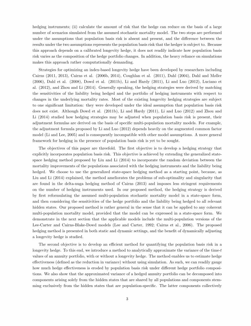
Table 1: A summary of the information about the variance components V1(t), . . . , V5(t). The definitions

of Ψ(PH)t , ~G

(PH)t and Γ

(PH)t are provided in equations (3.4), (3.6) and (3.5), respectively.

Component Relation with ~N(PH)t Associated hidden states Matrix notation

V1(t) Constant ~αct Not applicable

V2(t) Positive and quadratic ~αct ( ~N(PH)t )′Ψ

(PH)t

~N(PH)t

V3(t) Negative and linear ~αct −2(~G(PH)t )′ ~N

(PH)t

V4(t) Constant ~α(PL)t Not applicable

V5(t) Positive and quadratic ~α(PH)t ( ~N

(PH)t )′Γ

(PH)t

~N(PH)t

Overall, as the hedger acquires q-forwards, V3(t) reduces but V2(t) and V5(t) increase. If the reduction

in V3(t) outweighs the increase in V2(t) and V5(t), then the total variance of the hedged position reduces.

Furthermore, because the effects of V3(t) and the sum of V4(t) and V5(t) are offsetting, there exists an

optimal vector of notional amounts which would minimize the variance of the hedged position. In Table 1

we summarize how each variance component is related to the q-forwards’ notional amounts and the hidden

states. These relationships form the basis for the derivation of the optimal notional amounts in Section

3.3 and the further analysis of population basis risk in Section 4.

3.3 Deriving the Hedging Strategies

We now derive the optimal notional amounts that minimize Var(l(t) −∑mj=1N

(PH)j (t)h

(PH)j (t)), the ap-

proximated variance of the values of the hedged position. To facilitate the derivation, we first rewrite

V2(t), V3(t) and V5(t) in matrix forms. For V2(t) and V5(t), which are quadratically related to the notional

amounts, we have

V2(t) = ( ~N(PH)t )′Ψ

(PH)t

~N(PH)t ,

V5(t) = ( ~N(PH)t )′Γ

(PH)t

~N(PH)t ,

where Ψ(PH)t and Γ

(PH)t are m-by-m square matrices, with the (i, j)th element being

Ψ(PH)i,j|t =

(∂H

(PH)i (t)

∂~αct+Ti|t

)′Cov(~αct+Ti|t, ~α

ct+Tj |t)

∂H(PH)j (t)

∂~αct+Tj |t(3.4)

and

Γ(PH)i,j|t =

∂H(PH)i (t)

∂~α(PH)t+Ti|t

′ Cov(~α(PH)t+Ti|t, ~α

(PH)t+Tj |t)

∂H(PH)j (t)

∂~α(PH)t+Tj |t

, (3.5)

respectively. For V3(t), which is linearly related to the notional amounts, we have

V3(t) = −2(~G(PH)t )′ ~N

(PH)t ,

14

where ~G(PH)t is an m-by-1 vector with the jth element G

(PH)j (t) being

G(PH)j (t) =

t0+T∑s=t+1

(∂H

(PH)j (t)

∂~αct+Tj |t

)′Cov(~αct+Tj |t, ~α

cs|t)

∂L(t)

∂~αcs|t. (3.6)

We can then express the variance to be minimized as

Var

l(t)− m∑j=1

N(PH)j (t)h

(PH)j (t)

= ( ~N(PH)t )′(Ψ

(PH)t + Γ

(PH)t ) ~N

(PH)t − 2(~G

(PH)t )′ ~N

(PH)t +C(t), (3.7)

where C(t) = V1(t) + V4(t) is a constant that is free of the notional amounts.

To derive the optimal notional amounts, we take partial derivative of Var(l(t)−∑mj=1N

(PH)j (t)h

(PH)j (t))

with respect to ~N(PH)t , which gives

∂Var(l(t)−∑mj=1N

(PH)j (t)h

(PH)j (t))

∂ ~N(PH)t

= 2(Ψ(PH)t + Γ

(PH)t ) ~N

(PH)t − 2~G

(PH)t .

The optimal vector of notional amounts~N

(PH)t that minimizes Var(l(t) −

∑mj=1N

(PH)j (t)h

(PH)j (t)) can be

obtained readily by setting the partial derivative to zero:

(Ψ

(PH)t + Γ

(PH)t

)~N

(PH)t = ~G

(PH)t

~N

(PH)t =

(Ψ

(PH)t + Γ

(PH)t

)−1~G(PH)t .

(3.8)

The second step holds because, as discussed by Liu and Li (2014), Ψ(PH)t and Γ

(PH)t are positive-definite

matrices. Finally, the minimized value of Var(l(t)−∑mj=1N

(PH)j (t)h

(PH)j (t)) can be obtained by plugging

equation (3.8) into equation (3.7), which gives

minN

(PH )

1 (t),...,N(PH )m (t)

Var(l(t)−m∑j=1

N(PH)j (t)h

(PH)j (t))

= C(t)−(~G(PH)t )′

(Ψ

(PH)t + Γ

(PH)t

)−1~G(PH)t . (3.9)

Equations (3.8) and (3.9) involve Cov(~αcs|t, ~αcu|t), Cov(~α

(PL)s|t , ~α

(PL)u|t ) and Cov(~α

(PH)s|t , ~α

(PH)u|t ) for some

s, u > t. To compute these quantities, we first calculate the covariance matrix of ~αs|t and ~αu|t for s, u > t,

given the information up to and including time t, as

Ξs,u|t := Cov(~αs|t, ~αu|t) =

D|s−u|(Q+DQD′ + · · ·Du−(t+1)Q(Du−(t+1))′) , s > u

(Q+DQD′ + · · ·Ds−(t+1)Q(Ds−(t+1))′)(D|s−u|)′ , s < u

Q+DQD′ + · · ·Du−(t+1)Q(Du−(t+1))′ , s = u

.

15

Then Ξs,u|t is decomposed into (np + 1) block matrices as follows:

Ξs,u|t =

Cov(~αcs|t, ~αcu|t) 0 0 · · · 0

0 Cov(~α(1)s|t , ~α

(1)u|t) 0 · · · 0

0 0 Cov(~α(2)s|t , ~α

(2)u|t) · · · 0

......

.... . .

...

0 0 0 · · · Cov(~α(np)

s|t , ~α(np)

u|t )

.

Finally, Ξcs,u|t = Cov(~αcs|t, ~αcu|t), Ξ

(PL)s,u|t = Cov(~α

(PL)s|t , ~α

(PL)u|t ) and Ξ

(PH)s,u|t = Cov(~α

(PH)s|t , ~α

(PH)u|t ) can be obtained

respectively from the corresponding block matrices in Ξs,u|t.

Equations (3.8) and (3.9) also encompass the partial derivatives of L(t) and H(PH)j (t) with respect to

the common states and the population-specific states. The partial derivatives of L(t) with respect to ~αcs|t

and ~α(PL)s|t , evaluated at ~αcs|t = ~αcs|t and ~α

(PL)s|t = ~α

(PL)s|t , can be computed as

∂L(t)∂~αc

s|t=

T−(t−t0)∑u=s−t

e−ru

∂g(PL)

x0+s−t0−1,s|t

∂y(PL)

x0+s−t0−1,s|t

∣∣∣~αs|t=~αs|t

∂y(PL)

x0+s−t0−1,s|t∂~αc

s|t

∣∣∣~αs|t=~αs|t

t+u∏v=t+1v 6=s

g(PL)x0+v−t0−1,v|t

=

T−(t−t0)∑u=s−t

e−ru~bcx0+s−t0−1

∂g(PL)

x0+s−t0−1,s|t

∂y(PL)

x0+s−t0−1,s|t

∣∣∣~αs|t=~αs|t

t+u∏v=t+1v 6=s

g(PL)x0+v−t0−1,v|t

(3.10)

and

∂L(t)

∂~α(PL)

s|t

=T−(t−t0)∑u=s−t

e−ru

∂g(PL)

x0+s−t0−1,s|t

∂y(PL)

x0+s−t0−1,s|t

∣∣∣~αs|t=~αs|t

∂y(PL)

x0+s−t0−1,s|t

∂~α(PL)

s|t

∣∣∣~αs|t=~αs|t

t+u∏v=t+1v 6=s

g(PL)x0+v−t0−1,v|t

=

T−(t−t0)∑u=s−t

e−ru~b(PL)x0+s−t0−1

∂g(PL)

x0+s−t0−1,s|t

∂y(PL)

x0+s−t0−1,s|t

∣∣∣~αs|t=~αs|t

t+u∏v=t+1v 6=s

g(PL)x0+v−t0−1,v|t

,

(3.11)

respectively, where ~bcx and ~b(PL)x are defined in equation (2.3), and g

(PL)x,s|t is the value of g

(PL)x,s|t evaluated at

~αcs|t = ~αcs|t and ~α(PL)s|t = ~α

(PL)s|t . Similarly, the partial derivatives of H

(PH)j (t) with respect to ~αct+Tj |t and

~α(PH)t+Tj |t, evaluated at ~αct+Tj |t = ~αct+Tj |t and ~α

(PH)t+Tj |t = ~α

(PH)t+Tj |t, can be calculated as

∂H(PH )

j (t)

∂~αct+Tj |t

= e−rTj

∂g(PH )

xj,t+Tj |t

∂y(PH )

xj,t+Tj |t∣∣∣~αs|t=~αs|t

∂y

(PH )

xj,t+Tj |t

∂~αct+Tj |t

∣∣∣~αs|t=~αs|t

= e−rTj~bcxj

∂g(PH )

xj,t+Tj |t

∂y(PH )

xj,t+Tj |t∣∣∣~αs|t=~αs|t

(3.12)

16

and

∂H(PH )

j (t)

∂~α(PH )

t+Tj |t

= e−rTj

∂g(PH )

xj,t+Tj |t

∂y(PH )

xj,t+Tj |t∣∣∣~αs|t=~αs|t

∂y

(PH )

xj,t+Tj |t

∂~α(PH )

t+Tj |t∣∣∣~αs|t=~αs|t

= e−rTj~b

(PH)xj

∂g(PH )

xj,t+Tj |t

∂y(PH )

xj,t+Tj |t∣∣∣~αs|t=~αs|t

,

(3.13)

respectively, where ~bcx and ~b(PH)x are defined in equation (2.3).

The calculation of ∂g(p)x,s|t/∂y

(p)x,s|t in equations (3.10), (3.11), (3.12) and (3.13) depends on the specifica-

tion of the assumed model. For the ACF model (and other models that are built for central death rates),

we have

∂g(p)x,s|t

∂y(p)x,s|t

∣∣∣~αs|t=~αs|t

= − exp(y(p)x,s|t) exp(− exp(y

(p)x,s|t)) = −m(p)

x,s|t exp(−m(p)x,s|t), (3.14)

where m(p)x,s|t represents the value of m

(p)x,s|t evaluated at ~αcs|t = ~αcs|t and ~α

(p)s|t = ~α

(p)s|t . For the M-CBD model

(and other models that are built for single-year conditional death probabilities), we have

∂g(p)x,s|t

∂y(p)x,s|t

∣∣∣~αs|t=~αs|t

= −exp(y

(p)x,s|t)

(1 + exp(y(p)x,s|t))

2= −q(p)x,s|t

(1− q(p)x,s|t

), (3.15)

where q(p)x,s|t represents the value of q

(p)x,s|t evaluated at ~αcs|t = ~αcs|t and ~α

(p)s|t = ~α

(p)s|t .

3.4 Evaluation of Hedge Effectiveness

We evaluate hedge effectiveness by measuring the proportion of variance reduced. In the absence of any

longevity hedge, the time-t0 (random) value of the annuity liabilities is L(t0). If a static hedge with m

q-forwards is established at t = t0, then the hedger would receive offsetting cash flows from the q-forwards

at t = t0 + T1, . . . , t0 + Tm, which collectively have a time-t0 (random) value of∑mj=1N

(PH)j (t0)H

(PH)j (t0).

If the hedge is effective, then the offsetting cash flows would result in a hedged position that has a small

variance. Using this reasoning, we assess the hedge effectiveness of a static hedge with the following metric:

HE = 1−Var

(L(t0)−

∑mj=1N

(PH)j (t0)H

(PH)j (t0)

)Var(L(t0))

.

The value of HE is close to 1 if the longevity hedge is effective, and close to 0 if otherwise.

Using the approximation technique and the variance decomposition discussed in Section 3.2, we can

approximate HE as

HE = 1−Var

(l(t0)−

∑mj=1N

(PH)j (t0)h

(PH)j (t0)

)Var(l(t0))

= 1− V1(t0) + V2(t0) + V3(t0) + V4(t0) + V5(t0)

V1(t0) + V4(t0).

17

As shown in Section 3.2, all components (i.e., the covariance terms and the partial derivatives) in V1(t0),

V2(t0), V3(t0), V4(t0) and V5(t0) can be analytically computed. Hence, with minimal computational effort,

we can calculate HE for different combinations of notional amounts and derive an empirical relationship

between HE and N(PH)1 , . . . , N

(PH)m . This feature may be considered as an advantage over some of the

existing longevity hedging methods (Cairns, 2011, 2013; Cairns et al., 2014; Coughlan et al., 2011; Li and

Hardy, 2011), in which a simulation is required to calculate the hedge effectiveness for each combination

of notional amounts.

For a dynamic hedge, the cash flows from the hedge portfolio are more complicated because the hedger

does not hold the hedging instruments to maturity. In constructing a dynamic hedge, we assume that

at time t0 the hedger acquires m freshly launched q-forwards which have reference ages x1, . . . , xm and

times-to-maturity T1, . . . , Tm. Then, at each time point t = t0 + 1, . . . , t0 + T − 1, the hedger closes out all

of the q-forwards in the existing hedge portfolio, and acquires m freshly launched q-forwards which also

have reference ages x1, . . . , xm and times-to-maturity T1, . . . , Tm. Finally, at t = T , all of the q-forwards

in the hedge portfolio are closed out. We let PCF (t) be time-t0 value of the net cash flow that is incurred

when the hedger adjusts the hedge portfolio at time t. Given the assumptions we made, we can express

PCF (t) as follows:

PCF (t) = S(PH)x0,t0,t−1

m∑j=1

N(PH)j (t− 1)e−r(t−t0−1+Tj)(E(q

(PH)xj ,t−1+Tj |t−1)− E(q

(PH)xj ,t−1+Tj |t)) (3.16)

for t = t0 + 1, . . . , t0 + T , where

S(PH)x0,t0,t−1 =

{1, t = t0 + 1∏t−1s=t0+1(1− q(PH)

x0+s−t0−1,s|t−1), t = t0 + 2, . . . , t0 + T

represents the probability that an individual from the hedger’s population, who is aged x0 at time t0,

survives to time t − 1. The effectiveness for the dynamic hedge can then be assessed by the following

formula:

HE = 1−Var

(L(t0)−

∑t0+Tt=t0+1 PCF (t)|Ft0

)Var(L(t0)|Ft0)

.

4 Analyzing Population Basis Risk

The goal of this section is to investigate how the variance decomposition presented in Section 3.2 can help us

quantify population basis risk. We begin this section by studying the hedger’s risk exposure in a situation

when population basis risk is assumed to be absent. Then, we examine the effect of population basis risk

by observing how the hedger’s risk exposure would change when the assumption of no population basis risk

is relaxed. Finally, we develop a quantity called ‘standardized basis risk profile,’ which allows hedgers to

compare the levels of population basis risk arising from different reference populations. Throughout this

section, diagrams that aid us to understand population basis risk are presented.

18

4.1 The Hedger’s Risk Exposure when Population Basis Risk is Absent

Let us first consider a simplified scenario in which population basis risk is assumed to be absent. Under our

set-up, population basis risk arises solely from the population-specific states, so the simplified scenario can

be interpreted to mean the situation when the population-specific states are not stochastic. To construct the

simplified scenario, we set Q(p) = 0 for p = 1, 2, . . . , np, which implies the population-specific states would

remain constant; that is, ~α(p)s|t0 ≡ ~α

(p)t0|t0 , for p = 1, . . . , np and s ≥ t0. Consequently, Cov(~α

(PH)s|t , ~α

(PH)u|t ) = 0

for all s, u > t, and hence Γ(PH)t , V4(t) and V5(t) would become zero. In the simplified scenario, the total

longevity risk that the hedger is exposed to is V1(t) + V2(t) + V3(t).

When population basis risk is hypothetically absent, the choice of the q-forwards’ reference population

PH should not affect the optimal hedge effectiveness. In other words, the minimized variance specified

in equation (3.9) should not depend on PH . This fact can be verified mathematically as follows. Let us

rewrite the square matrix Ψ(PH)t in equation (3.7) as a product of three square matrices,

Ψ(PH)t = Λ

(PH)t ZctΛ

(PH)t , (4.1)

where Λ(PH)t is an m-by-m diagonal matrix with the jth diagonal element λ

(PH)j (t) being

λ(PH)j (t) = e−rTj

∂g(PH)xj ,t+Tj |t

∂y(PH)xj ,t+Tj |t

∣∣∣~αs|t=~αs|t

, (4.2)

and Zct is another m-by-m symmetric matrix with the (i, j)th element being

Zci,j(t) = (~bcxi)′Ξct+Ti,t+Tj |t

~bcxj. (4.3)

Similarly, we rewrite ~G(PH)t in equation (3.7) as a product of a square matrix and a vector,

~G(PH)t = Λ

(PH)t

~Gct , (4.4)

where ~Gct = (Gc1(t), . . . , Gcm(t))′ is an m-by-1 vector with the jth element Gcj(t) being

Gcj(t) =

t0+T∑s=t+1

(~bcxj)′Ξct+Tj ,s|t

∂L(t)

∂~αs|t.

The definition of~bcx is provided in equation (2.3). Note that neither Zct nor ~Gct depends on PH . Substituting

Γ(PH)t = 0 and equations (4.1) and (4.4) into equation (3.9), we obtain

minN

(PH )

1 (t),...,N(PH )m (t)

Var(l(t)−m∑j=1

N(PH)j (t)h

(PH)j (t))

= C(t)− (~Gct)′(Zct )

−1 ~Gct ,

which is free of PH .

Nevertheless, even if population basis risk is absent, the optimal notional amounts do depend on the

q-forwards’ reference population. The dependence of~N

(PH)t on PH can be seen by substituting Γ

(PH)t = 0

19

0

V1(t)

Notional Amount

p1

p2

p3

0

V1(t)

Standardized Notional Amount

Figure 1: The theoretical patterns of V1(t) + V2(t) + V3(t) as functions of the (non-standardized) notionalamount (the left panel) and the standardized notional amount (the right panel). It is assumed that oneq-forward is used and that the available reference populations are p1, p2 and p3.

and equations (4.1) and (4.4) into equation (3.8), which gives

~N

(PH)t = (Λ

(PH)t )−1(Zct )

−1 ~Gct . (4.5)

The dependence of~N

(PH)t on PH lies in the diagonal matrix Λ

(PH)t , which, according to equations (3.14) and

(3.15), contains either m(PH)x,s|t or q

(PH)x,s|t . This diagonal matrix is related to PH , because different reference

populations may have different expected levels of mortality even after controlling for age and time.

To facilitate comparison, we define a quantity called ‘standardized notional amount,’ which takes the

expected level of mortality into account. Let

~N (PH)t = (N (PH)

1 (t), . . . ,N (PH)m (t))′ = Λ

(PH)t

~N(PH)t

be the vector of standardized notional amounts. It follows from equation (4.5) that the optimal standardized

notional amounts~N (PH)t = Λ

(PH)t

~N

(PH)t = (Zct )

−1 ~Gct are free of PH . Furthermore, when written in terms

of ~N (PH)t , both V2(t) = ( ~N (PH)

t )′Zct ~N(PH)t and V3(t) = −2(~Gct)

′ ~N (PH)t have coefficients that do not depend

on PH .

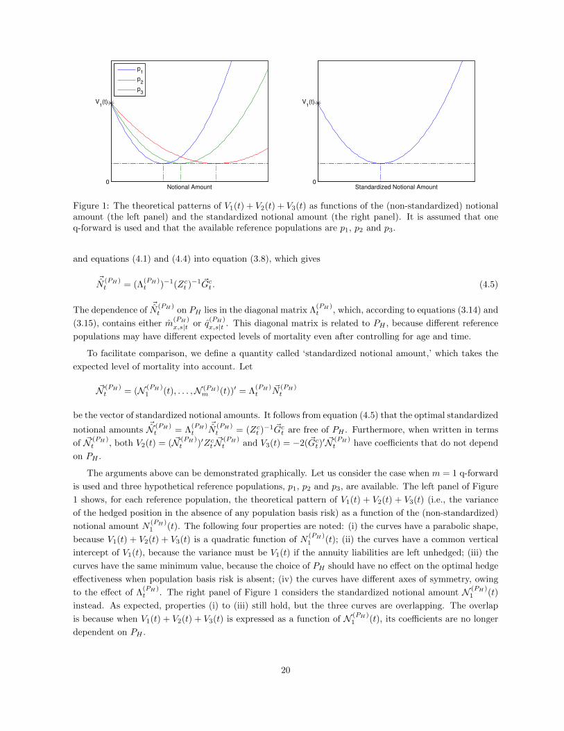
The arguments above can be demonstrated graphically. Let us consider the case when m = 1 q-forward

is used and three hypothetical reference populations, p1, p2 and p3, are available. The left panel of Figure

1 shows, for each reference population, the theoretical pattern of V1(t) + V2(t) + V3(t) (i.e., the variance

of the hedged position in the absence of any population basis risk) as a function of the (non-standardized)

notional amount N(PH)1 (t). The following four properties are noted: (i) the curves have a parabolic shape,

because V1(t) + V2(t) + V3(t) is a quadratic function of N(PH)1 (t); (ii) the curves have a common vertical

intercept of V1(t), because the variance must be V1(t) if the annuity liabilities are left unhedged; (iii) the

curves have the same minimum value, because the choice of PH should have no effect on the optimal hedge

effectiveness when population basis risk is absent; (iv) the curves have different axes of symmetry, owing

to the effect of Λ(PH)t . The right panel of Figure 1 considers the standardized notional amount N (PH)

1 (t)

instead. As expected, properties (i) to (iii) still hold, but the three curves are overlapping. The overlap

is because when V1(t) + V2(t) + V3(t) is expressed as a function of N (PH)1 (t), its coefficients are no longer

dependent on PH .

20

4.2 The Hedger’s Risk Exposure when Population Basis Risk is Present

When population basis risk is present, Γ(PH)t becomes non-zero and the hedger’s total exposure to longevity

risk is V1(t) + V2(t) + V3(t) + V4(t) + V5(t). To have a deeper understanding of the hedger’s risk exposure,

we rewrite Γ(PH)t as a product of three square matrices,

Γ(PH)t = Λ

(PH)t Z

(PH)t Λ

(PH)t ,

where Λ(PH)t is specified in equation (4.2) and Z

(PH)t is an m-by-m symmetric matrix with the (i, j)th

element being

Z(PH)i,j (t) = (~b(PH)

xi)′Ξ

(PH)t+Ti,t+Tj |t

~b(PH)xj

. (4.6)

The definition of ~b(PH)x is provided in equation (2.3). It immediately follows from equation (3.8) that the

optimal standardized notional amounts are given by

~N (PH)t = Λ

(PH)t

~N

(PH)t = (Zct + Z

(PH)t )−1 ~Gct . (4.7)

Also, it follows from equation (3.9) that the minimized variance can be expressed as

minN

(PH )

1 (t),...,N(PH )m (t)

Var(l(t)−m∑j=1

N(PH)j (t)h

(PH)j (t))

= C(t)− (~Gct)′(Zct + Z

(PH)t )−1 ~Gct . (4.8)

When population basis risk is present, Z(PH)t ,

~N (PH)t and the minimized variance are all related to

the q-forwards’ reference population PH . Moreover, because C(t), ~Gct and Zct do not depend on PH , the

dependence of~N (PH)t and the minimized variance on PH lies exclusively in Z

(PH)t . Therefore, Z

(PH)t should

contain all information concerning the population basis risk that arises from the difference in the mortality

improvements between the reference population PH and the hedger’s own population of individuals.

Let us consider the case when m = 1 q-forward is used. In this case, Z(PH)t reduces to a scalar and

equals

Z(PH)1,1 (t) = (~b(PH)

x1)′Ξ

(PH)t+T1,t+T1|t

~b(PH)x1

:= BRP (x1, T1, PH).

We call BRP (x1, T1, PH) the ‘standardized basis risk profile’ for a q-forward with reference age x1, time-

to-maturity T1 and reference population PH . This quantity is non-negative, because it can be regarded as

the variance of (~b(PH)x1 )′~α

(PH)t+T1|t. It can be observed from equation (4.8) that when m = 1, the minimized

variance is an increasing function of BRP (x1, T1, PH). A smaller value of BRP (x1, T1, PH) thus represents

a more favourable optimal hedging performance. Moreover, according to equation (4.7), when m = 1 the

optimal standardized notional amount is a decreasing function in BRP (x1, T1, PH). What this means is

that in the extreme case when BRP (x1, T1, PH) is very high, it is optimal not to hedge with the q-forward

with parameters x1, T1 and PH .

The connection between BRP (x1, T1, PH) and population basis risk can be understood from another

angle. According to the decomposition of variance presented in Section 3.2, population basis risk is rep-

resented by two components, V4(t) and V5(t), which are respectively related to the idiosyncratic features

of the hedger’s own population and the q-forwards’ reference population. Also, while V4(t) is a constant,

21

V5(t) is a quadratic function of the q-forwards’ notional amounts, reflecting the fact that the hedger is

exposed to more risk associated with the idiosyncratic features of the q-forwards’ reference population as

the notional amounts become larger. As a fact, when m = 1,

V5(t) = BRP (x1, T1, PH)× (N (PH)1 (t))2,

which means that BRP (x1, T1, PH) can be understood as the speed at which population basis risk grows

when the (standardized) notional amount of the q-forward with parameters x1, T1 and PH increases. It is

clear that other things equal, a hedger should choose a q-forward with the lowest value of BRP (x1, T1, PH).

In practice, the standardized basis risk profile can aid hedgers to select the most appropriate reference

population out of the reference populations available in the market. While the methods proposed previously

by Cairns (2011, 2013), Cairns et al. (2014), Coughlan et al. (2011) and Li and Hardy (2011) may also

be used for the purpose of reference population selection, they generally require a lot more computational

effort because they involve multiple steps: (i) for each candidate reference population, calibrate the hedge

(i.e., select the optimal notional amounts); (ii) simulate realizations of future mortality and calculate the

hedge effectiveness resulting from each calibrated hedge; (iii) choose the reference population that leads to

the best hedge effectiveness. In contrast, the standardized basis risk profile can be computed analytically,

and the comparison between different standardized basis risk profiles can be made without calibrating the

associated hedges in advance.

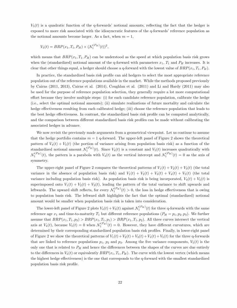
We now revisit the previously made arguments from a geometrical viewpoint. Let us continue to assume

that the hedge portfolio contains m = 1 q-forward. The upper-left panel of Figure 2 shows the theoretical

pattern of V4(t) + V5(t) (the portion of variance arising from population basis risk) as a function of the

standardized notional amount N (PH)1 (t). Since V4(t) is a constant and V5(t) increases quadratically with

N (PH)1 (t), the pattern is a parabola with V4(t) as the vertical intercept and N (PH)

1 (t) = 0 as the axis of

symmetry.

The upper-right panel of Figure 2 compares the theoretical patterns of V1(t) + V2(t) + V3(t) (the total

variance in the absence of population basis risk) and V1(t) + V2(t) + V3(t) + V4(t) + V5(t) (the total

variance including population basis risk). As population basis risk is being incorporated, V4(t) + V5(t) is

superimposed onto V1(t) + V2(t) + V3(t), leading the pattern of the total variance to shift upwards and

leftwards. The upward shift reflects, for every N (PH)1 (t) > 0, the loss in hedge effectiveness that is owing

to population basis risk. The leftward shift highlights the fact that the optimal (standardized) notional

amount would be smaller when population basis risk is taken into consideration.

The lower-left panel of Figure 2 plots V4(t) +V5(t) against N (PH)1 (t) for three q-forwards with the same

reference age x1 and time-to-maturity T1 but different reference populations (PH = p1, p2, p3). We further

assume that BRP (x1, T1, p3) > BRP (x1, T1, p1) > BRP (x1, T1, p2). All three curves intersect the vertical

axis at V4(t), because V5(t) = 0 when N (PH)1 (t) = 0. However, they have different curvatures, which are

determined by their corresponding standardized population basis risk profiles. Finally, in lower-right panel

of Figure 2 we show the theoretical patterns of V1(t) +V2(t) +V3(t) +V4(t) +V5(t) for the three q-forwards

that are linked to reference populations p1, p2 and p3. Among the five variance components, V5(t) is the

only one that is related to PH and hence the differences between the shapes of the curves are due entirely

to the differences in V5(t) or equivalently BRP (x1, T1, PH). The curve with the lowest vertex (which means

the highest hedge effectiveness) is the one that corresponds to the q-forward with the smallest standardized

population basis risk profile.

22

0

V4(t)

Standardized Notional Amount

V4(t)+V

5(t)

0

V1(t)

V1(t)+V

4(t)

Standardized Notional Amount

V1(t)+V

2(t)+V

3(t)+V

4(t)+V

5(t)

V1(t)+V

2(t)+V

3(t)

0

V4(t)

Standardized Notional Amount

p1

p2

p3

0

V1(t)+V

4(t)

Standardized Notional Amount

p1

p2

p3

Figure 2: The theoretical relationships between different combinations of variance components and thestandardized notional amount of the q-forward in a single-instrument hedge portfolio;upper-left: V4(t) + V5(t);upper-right: V1(t) + V2(t) + V3(t) and V1(t) + V2(t) + V3(t) + V4(t) + V5(t);lower-left: V4(t) + V5(t) for hypothetical reference populations p1, p2, p3;lower-right: V1(t) + V2(t) + V3(t) + V4(t) + V5(t) for hypothetical reference populations p1, p2, p3.

5 A Numerical Illustration

In this section, we illustrate the proposed methods with some real mortality data. We begin this section by

stating the general assumptions made. We then present the estimated multi-population mortality model on

which the illustrative longevity hedges are based. Finally, the results of the illustrative static and dynamic

longevity hedges are discussed in turn.

5.1 Assumptions

The following assumptions are made throughout the rest of this section.

• The liability being hedged is a portfolio of 30-year temporary life annuity immediate contracts that

are sold to persons aged 60 at time t0; that is x0 = 60 and T = 30.

• The annuitants’ mortality is exactly the same as that of Canadian males.

23

Table 2: The estimates of the parameters in the transition equation of the ACF model.

~U D Qµc −3.7903× 10−1 − − Qc 1.0739× 10−1

µ(1) −2.5276× 10−3 φ(1) 9.0759× 10−1 Q(1) 1.5802× 10−3

µ(2) −4.9883× 10−3 φ(2) 9.0310× 10−1 Q(2) 1.4631× 10−1

µ(3) −1.1591× 10−1 φ(3) 9.3293× 10−1 Q(3) 5.9729× 10−1

µ(4) 6.1779× 10−2 φ(4) 9.4680× 10−1 Q(4) 3.1499× 10−1

µ(5) −3.3226× 10−2 φ(5) 9.1873× 10−1 Q(5) 2.0034× 10−1

• There is no small sample risk.

• The hedge portfolio is composed of only m = 1 q-forward, which has a reference age of x1 = 60 and

a time-to-maturity (from the launch date) of T1 = 10.

• In the market, q-forwards that are linked to the male populations of the following four countries are

available and liquidly traded: the US, England and Wales, the Netherlands and West Germany. We

make this assumption because the tradable LifeMetrics Indexes offered by the LLMA are linked to

each of these four national populations. There is no q-forward linked to the population of Canadian

males.

• The continuously compounded interest rate (r) is assumed to be 0.01 per annum.

• There is no transaction cost.

5.2 The Multi-Population Mortality Model Used

Given the assumptions made, we require a mortality model for np = 5 populations. The model we use is the

ACF model discussed in Section 2.2. We estimate the model to the historical mortality data of Canadian

males (p = 1), US males (p = 2), English and Welsh males (p = 3), Dutch males (p = 4) and West German

males (p = 5), using the method of maximum likelihood with the following identifiability constraints:∑xb

x=xabcx = 1,

∑xb

x=xab(p)x = 1 for p = 1, . . . , np,

∑tbt=ta

kct = 0, and∑tbt=ta

k(p)t = 0 for p = 1, . . . , np. The

sample age range [xa, xb] and calibration window [ta, tb] used are [60, 89] and [1961, 2009], respectively. All

required data are obtained from the Human Mortality Database (2015).

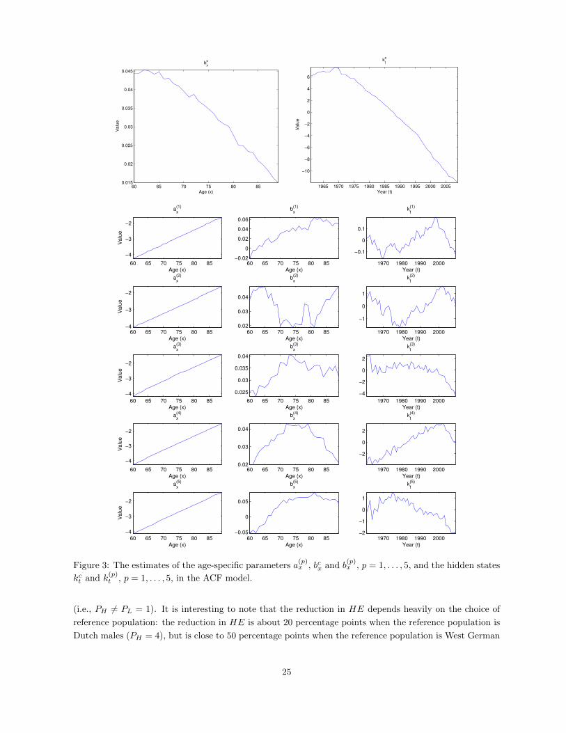
The estimates of the age-specific parameters in the observation equation and the hidden states over the

calibration window are shown graphically in Figure 3. The estimates of the parameters in the transition

equation are provided in Table 2.

In what follows, we set t0 to the end of 2009, the last year of the calibration window. Also, following

the assumptions made in Section 5.1, PL = 1 and the possible values of PH are 2, 3, 4 and 5.

5.3 Hedging Results I: Static Hedges

In this sub-section we consider static hedges that are established at time t0 and are left unadjusted af-

terwards. Table 3 compares the resulting values of HE (calculated by simulation) when population basis

risk is absent and present. The value of HE is close to 80% in the ideal world where population basis

risk is non-existent, but reduces to 30-60% in a more realistic situation when population basis risk exists

24

60 65 70 75 80 850.015

0.02

0.025

0.03

0.035

0.04

0.045

Va

lue

Age (x)

bx

c

1965 1970 1975 1980 1985 1990 1995 2000 2005

−10

−8

−6

−4

−2

0

2

4

6

Va

lue

Year (t)

kt

c

60 65 70 75 80 85

−4

−3

−2

Age (x)

Valu

e

ax

(1)

60 65 70 75 80 85−4

−3

−2

Age (x)

Valu

e

ax

(2)

60 65 70 75 80 85

−4

−3

−2

Age (x)

Valu

e

ax

(3)

60 65 70 75 80 85

−4

−3

−2

Age (x)

Valu

e

ax

(4)

60 65 70 75 80 85

−4

−3

−2

Age (x)

Valu

e

ax

(5)

60 65 70 75 80 85−0.02

0

0.02

0.04

0.06

Age (x)

bx

(1)

60 65 70 75 80 850.02

0.03

0.04

Age (x)

bx

(2)

60 65 70 75 80 85

0.025

0.03

0.035

0.04

Age (x)

bx

(3)

60 65 70 75 80 850.02

0.03

0.04

Age (x)

bx

(4)

60 65 70 75 80 85−0.05

0

0.05

Age (x)

bx

(5)

1970 1980 1990 2000

−0.1

0

0.1

Year (t)

kt

(1)

1970 1980 1990 2000

−1

0

1

Year (t)

kt

(2)

1970 1980 1990 2000

−4

−2

0

2

Year (t)

kt

(3)

1970 1980 1990 2000

−2

0

2

Year (t)

kt

(4)

1970 1980 1990 2000−2

−1

0

1

Year (t)

kt

(5)

Figure 3: The estimates of the age-specific parameters a(p)x , bcx and b

(p)x , p = 1, . . . , 5, and the hidden states

kct and k(p)t , p = 1, . . . , 5, in the ACF model.

(i.e., PH 6= PL = 1). It is interesting to note that the reduction in HE depends heavily on the choice of

reference population: the reduction in HE is about 20 percentage points when the reference population is

Dutch males (PH = 4), but is close to 50 percentage points when the reference population is West German

25

Table 3: The values of HE (calculated by simulation) and HE (the analytical approximation of HE) whenpopulation basis risk is absent and present.

Basis risk is absentBasis risk is present

PH = 2 PH = 3 PH = 4 PH = 5HE (calculated by simulation) 0.7905 0.5393 0.3816 0.5794 0.3159

HE (calculated analytically) 0.7902 0.5352 0.3860 0.5725 0.3155

Table 4: The component variances, V1(t0), . . . , V5(t0), when population basis risk is assumed to be absent.

V1(t0) V2(t0) V3(t0) V4(t0) V5(t0)An optimized hedge with 1 q-forward 0.0249 0.0197 −0.0393 0.0000 0.0000

No hedge 0.0249 0.0000 0.0000 0.0000 0.0000

males (PH = 5). This result suggests that it is important to choose the q-forward’s reference population

carefully.

Also shown in Table 3 are the values of HE, the analytical approximation of HE. For all five cases, the

values of HE are very close to the corresponding simulated values of HE, suggesting that the analytical

approximation is reasonably accurate and may hence be used in practice to save computational effort.

We now move to studying the component risks: V1(t0), . . . , V5(t0). As discussed in Sections 3.2 and

3.3, they can be computed analytically. Let us first consider the situation when population basis risk is

assumed to be absent (Table 4). In such a situation, all population-specific states are non-stochastic, so that

V4(t0) = V5(t0) = 0 regardless of the q-forward’s notional amount. When the liabilities are left unhedged,

V2(t0) = V3(t0) = 0 while V1(t0) = 0.0249 > 0, so that the total risk is 0.0249. If an optimized hedge is

in place, then V2(t0) becomes positive but V3(t0) becomes negative and larger than V2(t0) in magnitude.

In effect, the total risk, V1(t0) + V2(t0) + V3(t0), is reduced to 0.0053 (which is significantly smaller than

0.0249).

When there is no population basis risk, the value of HE is 0.7905 and the optimized standardized

notional amount N (PH)1 (t0) is 3.0537 no matter which reference population PH is chosen. However, for the

reasons provided in Section 4.2, the optimized (non-standardized) notional amounts do depend on PH . In

particular, we have N(2)1 (t0) = 395.0998, N

(3)1 (t0) = 476.3772, N

(4)1 (t0) = 489.7257, N

(5)1 (t0) = 401.9512.

These results can be visualized in Figure 4, which shows how V1(t0) + V2(t0) + V3(t0) (i.e., the total

longevity risk that the hedger is exposed to when there is no population basis risk) varies with N (PH)1 (t0)

and N(PH)1 (t0) for different choices of PH .

Next, we consider a more realistic situation when population basis risk is present (Table 5). In this

situation, V4(t0) is positive and is invariant with both the notional amount of the q-forward and the choice

of the q-forward’s reference population. The value of V4(t0) (0.0001) reflects the portion of population basis

risk arising from the hidden states that are associated with the hedger’s own population PL. On the other

hand, V5(t0) is zero when the liabilities are left unhedged but becomes positive as a q-forward contract is

acquired. The value of V5(t0) depends on PH , reflecting the portion of population basis risk arising from

the hidden states that are associated with the q-forward’s reference population.

It can be observed from Table 5 that the choice of reference population has a huge impact on the values

of V2(t0), V3(t0) and V5(t0) and consequently the hedge effectiveness. This outcome may be understood by

studying Figure 5, which shows the following three curves for each of the candidate reference populations:

26

0 100 200 300 400 500 600 7000

0.01

0.02

0.03

0.04

0.05

0.06

Notional Amount

Va

lue

PH

=2 (US)

PH

=3 (England and Wales)

PH

=4 (The Netherlands)

PH

=5 (West Germany)

0 1 2 3 4 5 6 70

0.01

0.02

0.03

0.04

0.05

0.06

Standardized Notional Amount

Va

lue

PH

=2 (US)

PH

=3 (England and Wales)

PH

=4 (The Netherlands)

PH

=5 (West Germany)

Figure 4: The relationship between V1(t0) + V2(t0) + V3(t0) and N(PH)1 (t0) (the left panel), and the rela-

tionship between V1(t0) + V2(t0) + V3(t0) and N (PH)1 (t0) (the right panel); PH = 2, 3, 4, 5.

(I) V1(t0) + V2(t0) + V3(t0) against the standardized notional amount N (PH)1 (t0);

(II) V4(t0) + V5(t0) against the standardized notional amount N (PH)1 (t0);

(III) V1(t0) + V2(t0) + V3(t0) + V4(t0) + V5(t0) against the standardized notional amount N (PH)1 (t0).

As previously explained, Curve (I) for all reference populations must be identical (see also the right

panel of Figure 4). For different reference populations, the vertical intercepts of Curve (II) are the same

(with a value of V4(t0) = 0.0001) but the curvatures of Curve (II) are not. Because Curve (III) is the

superimposition of Curves (I) and (II), the shape and position of Curve (III) depend on PH . In particular,

if the curvature of Curve (II) for a certain reference population is steeper, that is, the marginal increment

in population basis risk per unit standardized notional amount acquired is higher, then the vertex of

Curve (III) for the reference population would be positioned relatively higher and lefter. Therefore, for a

reference population with a steeper Curve (II), the minimized variance is higher (which corresponds to a

smaller value of HE) and the optimized standardized notional amount is smaller (which corresponds to

smaller magnitudes of V2(t0) and V3(t0) as the magnitudes of these two components are positively related

to N (PH)1 (t0)).

It is now clear that the relative degree of population basis risk depends entirely on the curvature of

Curve (II). Figure 6 displays each candidate reference population’s Curve (II). For each PH , the order

of the curvature of its Curve (II) is exactly the same as the order of its resulting population basis risk

(measured in terms of the reduction in HE; see Table 3). Recall that the standardized basis risk profile

BRP (x1, T1, PH) is defined as the curvature of Curve (II). Hence, instead of a graphical mean, one may

use this quantity to choose the reference population that would lead to the smallest amount of population

basis risk.

5.4 Hedging Results II: Dynamic Hedges

In this sub-section we consider dynamic hedges that are adjusted annually. In more detail, it is assumed

that at time t0, the hedger writes a N(PH)1 (t0) notional q-forward with reference age x1, time-to-maturity

T1 and reference population PH . Then, at each future time t, where t = t0 + 1, . . . , t0 + T − 1, the hedger

27

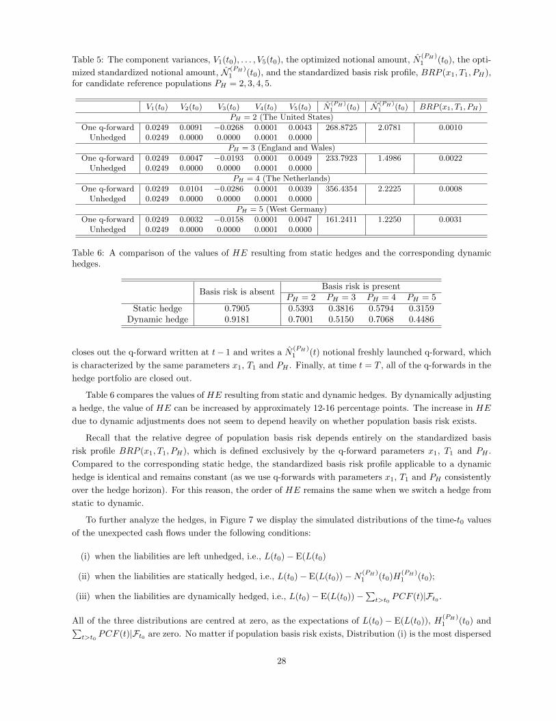
Table 5: The component variances, V1(t0), . . . , V5(t0), the optimized notional amount, N(PH)1 (t0), the opti-

mized standardized notional amount, N (PH)1 (t0), and the standardized basis risk profile, BRP (x1, T1, PH),

for candidate reference populations PH = 2, 3, 4, 5.

V1(t0) V2(t0) V3(t0) V4(t0) V5(t0) N(PH )1 (t0) N (PH )

1 (t0) BRP (x1, T1, PH)

PH = 2 (The United States)

One q-forward 0.0249 0.0091 −0.0268 0.0001 0.0043 268.8725 2.0781 0.0010Unhedged 0.0249 0.0000 0.0000 0.0001 0.0000

PH = 3 (England and Wales)

One q-forward 0.0249 0.0047 −0.0193 0.0001 0.0049 233.7923 1.4986 0.0022Unhedged 0.0249 0.0000 0.0000 0.0001 0.0000

PH = 4 (The Netherlands)

One q-forward 0.0249 0.0104 −0.0286 0.0001 0.0039 356.4354 2.2225 0.0008Unhedged 0.0249 0.0000 0.0000 0.0001 0.0000

PH = 5 (West Germany)

One q-forward 0.0249 0.0032 −0.0158 0.0001 0.0047 161.2411 1.2250 0.0031Unhedged 0.0249 0.0000 0.0000 0.0001 0.0000

Table 6: A comparison of the values of HE resulting from static hedges and the corresponding dynamichedges.

Basis risk is absentBasis risk is present

PH = 2 PH = 3 PH = 4 PH = 5Static hedge 0.7905 0.5393 0.3816 0.5794 0.3159

Dynamic hedge 0.9181 0.7001 0.5150 0.7068 0.4486

closes out the q-forward written at t− 1 and writes a N(PH)1 (t) notional freshly launched q-forward, which

is characterized by the same parameters x1, T1 and PH . Finally, at time t = T , all of the q-forwards in the

hedge portfolio are closed out.

Table 6 compares the values of HE resulting from static and dynamic hedges. By dynamically adjusting

a hedge, the value of HE can be increased by approximately 12-16 percentage points. The increase in HE

due to dynamic adjustments does not seem to depend heavily on whether population basis risk exists.

Recall that the relative degree of population basis risk depends entirely on the standardized basis

risk profile BRP (x1, T1, PH), which is defined exclusively by the q-forward parameters x1, T1 and PH .

Compared to the corresponding static hedge, the standardized basis risk profile applicable to a dynamic

hedge is identical and remains constant (as we use q-forwards with parameters x1, T1 and PH consistently

over the hedge horizon). For this reason, the order of HE remains the same when we switch a hedge from

static to dynamic.

To further analyze the hedges, in Figure 7 we display the simulated distributions of the time-t0 values

of the unexpected cash flows under the following conditions:

(i) when the liabilities are left unhedged, i.e., L(t0)− E(L(t0)

(ii) when the liabilities are statically hedged, i.e., L(t0)− E(L(t0))−N (PH)1 (t0)H

(PH)1 (t0);

(iii) when the liabilities are dynamically hedged, i.e., L(t0)− E(L(t0))−∑t>t0

PCF (t)|Ft0 .

All of the three distributions are centred at zero, as the expectations of L(t0) − E(L(t0)), H(PH)1 (t0) and∑

t>t0PCF (t)|Ft0 are zero. No matter if population basis risk exists, Distribution (i) is the most dispersed

28

0 1 2 3 4 5 6 70

0.01

0.02

0.03

0.04

0.05

0.06

Standardized Notional Amount

Valu

e

V1(t)+V

2(t)+V

3(t)

V4(t)+V

5(t)

V1(t)+V

2(t)+V

3(t)+V

4(t)+V

5(t)

(a) PH = 2

0 1 2 3 4 5 6 70

0.01

0.02

0.03

0.04

0.05

0.06

Standardized Notional Amount

Valu

e

V1(t)+V

2(t)+V

3(t)

V4(t)+V

5(t)

V1(t)+V

2(t)+V

3(t)+V

4(t)+V

5(t)

(b) PH = 3

0 1 2 3 4 5 6 70

0.01

0.02

0.03

0.04

0.05

0.06

Standardized Notional Amount

Valu

e

V1(t)+V

2(t)+V

3(t)

V4(t)+V

5(t)

V1(t)+V

2(t)+V

3(t)+V

4(t)+V

5(t)

(c) PH = 4

0 1 2 3 4 5 6 70

0.01

0.02

0.03

0.04

0.05

0.06

Standardized Notional Amount

Valu

e

V1(t)+V

2(t)+V

3(t)

V4(t)+V

5(t)

V1(t)+V

2(t)+V

3(t)+V

4(t)+V

5(t)

(d) PH = 5

Figure 5: The curves of (I) V1(t0) +V2(t0) +V3(t0), (II) V4(t0) +V5(t0), and (III) V1(t0) +V2(t0) +V3(t0) +

V4(t0) + V5(t0) against the standardized notional amount N (PH)1 (t0), PH = 2, 3, 4, 5.

while Distribution (iii) is the least. This observation indicates that a static hedge reduces the variability

of the unexpected cash flows and that the corresponding dynamic hedge reduces the variability even more.

Of course, the reductions in the variability of the unexpected cash flows are the most prominent when

population basis risk is assumed to be absent. When population basis risk is present, the reductions in the

variability of the unexpected cash flows depend quite significantly on PH .

6 Concluding Remarks

It is believed that hedgers’ concern about population basis risk is a major obstacle to the development of

the market for index-based longevity risk transfers. In 2013, the LLMA established the Longevity Basis

Risk Working Group, whose goal is to develop readily applicable methods for quantifying population basis

risk. This paper addresses the needs of the market by introducing a method for measuring population

basis risk efficiently and a framework for optimizing index-based longevity hedges when the index used is

associated with a population that is different from the hedger’s own population.

29

0 1 2 3 4 5 6 70

0.01

0.02

0.03

0.04

0.05

0.06

Standardized Notional Amount

Va

lue

PH

=2 (US)

PH

=3 (England and Wales)

PH

=4 (The Netherlands)

PH

=5 (West Germany)

Figure 6: V4(t0) + V5(t0) against the standardized notional amount N (PH)1 (t0), PH = 2, 3, 4, 5.

The first contribution of this paper is an extension of the generalized state-space hedging method

proposed by Liu and Li (2014). The extension allows us to calibrate a longevity hedge that is composed

of standardized hedging instruments, taken into account the difference in mortality improvements between

the populations associated with the hedging instruments and the hedger’s portfolio. The extension may

be regarded as a general framework, because it is applicable to all coherent multi-population stochastic

mortality models that can be written in state-space representations. We have demonstrated empirically

that when calibrated by the proposed method, a static longevity hedge with one q-forward can yield an

effectiveness of 30-60%, depending on the choice of the reference population. The effectiveness would

become 12 to 16 percentage points higher if the hedge is adjusted annually over the hedging horizon.

The second contribution is a method to analytically approximate the variances of L(t) (the time-t value

of unhedged position) and L(t)−∑mj=1N

(PH)j (t)H

(PH)j (t) (the time-t value of the hedged position). This

approximation method enables us to calculate the hedge effectiveness,

HE = 1−Var

(L(t0)−

∑mj=1N

(PH)j (t0)H

(PH)j (t0)

)Var(L(t0))

,

without using simulation. Using this approximation method, we can derive an empirical relationship be-

tween HE and the composition of the hedge portfolio (N(PH)1 (t), . . . , N

(PH)m (t)) with only minimal compu-

tational effort. Furthermore, by applying this approximation method to the full multi-population mortality

model and the restricted model with Q(1) = Q(2) = . . . = Q(np) = 0, we can readily gauge to what extend

population basis risk erodes hedge effectiveness under different hedge portfolio compositions.

The third contribution is an analysis of longevity risk through a variance decomposition. We have shown

that the (approximated) variance of the time-t values of a hedged annuity portfolio can be expressed as the

30

−1 −0.8 −0.6 −0.4 −0.2 0 0.2 0.4 0.6 0.8 10

0.5

1

1.5

2

2.5

3

3.5

Present value of unexpected cash flows

Density

Unhedged

Statically hedged

Dynamically hedged

No population basis risk

−1 −0.8 −0.6 −0.4 −0.2 0 0.2 0.4 0.6 0.8 10

0.5

1

1.5

2

2.5

3

3.5

Present value of unexpected cash flows

Density

Unhedged

Statically hedged

Dynamically hedged

−1 −0.8 −0.6 −0.4 −0.2 0 0.2 0.4 0.6 0.8 10

0.5

1

1.5

2

2.5

3

3.5

Present value of unexpected cash flows

Density

Unhedged

Statically hedged

Dynamically hedged

PH = 2 PH = 3

−1 −0.8 −0.6 −0.4 −0.2 0 0.2 0.4 0.6 0.8 10

0.5

1

1.5

2

2.5

3

3.5

Present value of unexpected cash flows

Density

Unhedged

Statically hedged

Dynamically hedged

−1 −0.8 −0.6 −0.4 −0.2 0 0.2 0.4 0.6 0.8 10

0.5

1

1.5

2

2.5

3

3.5

Present value of unexpected cash flows

Density

Unhedged

Statically hedged

Dynamically hedged

PH = 4 PH = 5

Figure 7: The simulated distributions of the time-t0 values of the unexpected cash flows when the liabilitiesare unhedged, statically hedged and dynamically hedged.

31

sum of five components, V1(t)+V2(t)+V3(t)+V4(t)+V5(t). We have argued that V4(t) and V5(t) collectively

represent an explicit measure of the population basis risk involved in the longevity hedge. In particular,

V4(t) represents the portion of population basis risk that exists no matter how the hedge is composed,

whereas V5(t) represents the portion of population basis risk that depends on the composition of the hedge

portfolio. We have also shown that V5(t) increases quadratically with the standardized notional amounts

N (PH)1 (t), . . . ,N (PH)

m (t) of the q-forwards used, and that the curvature depends on the parameters of the

q-forwards. Using these properties, we define a metric called standardized basis risk profile, which allows

us to assess the relative levels of population basis risk that q-forwards with different reference populations,

reference ages and times-to-maturity may lead to.

We conclude with the caveats of our work and suggestions for future research. The hedge effectiveness

reported in this paper does not take model and parameter risks into account. If the true underlying model is

not identical to the model used in deriving the general state-space hedging strategy, the hedge effectiveness

may be reduced. To estimate the possible reduction, one may recalculate hedge effectiveness by simulating

mortality scenarios generated by alternative multi-population mortality models. Similarly, the impact of

parameter risk can be estimated by recomputing hedge effectiveness using mortality scenarios that are

generated by bootstrapping or Bayesian methods (Brouhns et al., 2005; Cairns et al., 2011; Yang et al.,

2015).

It should also be noted that small sample risk (a.k.a. Poisson risk and sampling risk) is not incorporated

into the results of this paper. One may estimate the impact of small sample risk by simulation approaches,

in which realizations of death counts are simulated from a certain counting distribution such as Poisson

and binomial (Cairns et al., 2014; Li and Hardy, 2011). It may also be possible to estimate the impact of

small sample risk by analytical means. In more detail, when small sample risk is considered, the variance

of L(t) would consist additionally a component representing the variance of the time-t values of the future

liabilities given known values of q(PL)x0+t−t0 , q

(PL)x0+t+1−t0 , . . .. If this component can be analytically computed

or approximated, then we can obtain an analytical approximation of HE that incorporates small sample

risk. The derivation of such an analytical expression is left for future research.

Acknowledgments

This work is supported by the Global Risk Institute, the Society of Actuaries Center of Actuarial Excellence

Programme and the Natural Sciences and Engineering Research Council of Canada.

References

Ahmadi, S. and Li, J.S.-H. (2014). Coherent Mortality Forecasting with Generalized Linear Models: A Modified

Time-Transformation Approach. Insurance: Mathematics and Economics 59: 194-221.

Blake, D., Cairns, A., Dowd, K. and MacMinn, R., (2006). Longevity Bonds: Financial Engineering, Valuation,

and Hedging. Journal of Risk and Insurance 73: 647-672.

Blake, D., Cairns, A., Coughlan, G., Dowd, K., and MacMinn, R. (2013). The New Life Market. Journal of Risk

and Insurance 80: 501-557.

Brouhns, N., Denuit, M., and Van Keilegom, I. (2005). Bootstrapping the Poisson Log-Bilinear Model for Mortality

Forecasting. Scandinavian Actuarial Journal 2005(3): 212-224.

32

Cairns, A.J.G. (2011). Modelling and Management of Longevity Risk: Approximations to Survival Functions and

Dynamic Hedging. Insurance: Mathematics and Economics 49: 438-453.

Cairns, A.J.G. (2013). Robust Hedging of Longevity Risk. Journal of Risk and Insurance 80: 621-648.

Cairns, A.J.G., Blake, D. and Dowd, K., (2006) A Two-Factor Model for Stochastic Mortality with Parameter

Uncertainty: Theory and Calibration. Journal of Risk and Insurance 73: 687-718.

Cairns, A.J.G., Blake, D., Dowd, K. and Coughlan, G.D. (2014). Longevity Hedge Effectiveness: A Decomposition.

Quantitative Finance 14: 217-235.

Cairns, A.J.G., Blake, D., Dowd, K., Coughlan, G.D. and Khalaf-Allah, M. (2011). Bayesian Stochastic Mortality

Modelling for Two Populations. ASTIN Bulletin 41: 29-59.

Canadian Institute of Actuaries (2014). Final Report on Canadian Pensioners’ Mortality. Available at

http://www.cia-ica.ca/docs/default-source/2014/214013e.pdf.

Continuous Mortality Investigation Bureau (2009a). Working Papers 38, A Prototype Mortality Projections

Model, Part One – An Outline of the Proposed Approach. Available at

http://www.actuaries.org.uk/research-and-resources/documents/cmi-working-paper-38-prototype-mortality-

projections-model-part-one.

Continuous Mortality Investigation Bureau (2009b). Working Papers 39, A Prototype Mortality Projections

Model, Part Two – Detailed Analysis. Available at

http://www.actuaries.org.uk/research-and-resources/documents/cmi-working-paper-39-prototype-mortality-

projections-model-part-two.

Coughlan, G.D., Khalaf-Allah, M., Ye, Y., Kumar, S., Cairns, A.J.G., Blake, D. and Dowd, K. (2011). Longevity

Hedging 101: A Framework for Longevity Basis Risk Analysis and Hedge Effectiveness. North American

Actuarial Journal 15: 150-176.

Dahl, M. (2004). Stochastic Mortality in Life Insurance: Market Reserves and Mortality-Linked Insurance Con-

tracts. Insurance: Mathematics and Economics 35: 113-136.

Dahl, M., Melchior, M. and Møller, T. (2008). On Systematic Mortality Risk and Risk Minimization with Mortality

Swaps. Scandinavian Actuarial Journal 108: 114-146.

Dahl, M. and Møller, T. (2006). Valuation and Hedging of Life Insurance Liabilities with Systematic Mortality

Risk. Insurance: Mathematics and Economics 39: 193-217.

D’Amato, V., Haberman, S., Piscopo, G., Russolillo, M., and Trapani, L. (2014). Detecting Common Longevity

Trends by a Multiple Population Approach. North American Actuarial Journal 18: 139-149.

Dowd, K., Cairns, A.J.G., Blake, D., Coughlan, G.D., Epstein, D. and Khalaf-Allah, M. (2011a). A Gravity Model

of Mortality Rates for Two Related Populations. North American Actuarial Journal 15: 331-356.

Dowd, K., Blake, D., Cairns, A.J.G. and Coughlan, G.D. (2011b). Hedging Pension Risks with the Age-Period-

Cohort Two-Population Gravity Model. In: Seventh International Longevity Risk and Capital Markets

Solutions Conference, Frankfurt, September 2011.

Graziani, G. (2014). Longevity risk - A Fine Balance. Institutional Investor Journals: Special Issue on Pension

and Longevity Risk Transfer for Institutional Investors 2014: 35-27.

Hatzopoulos, P. and Haberman, S. (2013). Common Mortality Modeling and Coherent Forecasts. An Empirical

Analysis of Worldwide Mortality Data. Insurance: Mathematics and Economics 52: 320-337.

33

Human Mortality Database. University of California, Berkeley (USA), and Max Planck Institute of Demographic

Research (Germany). Available at www.mortality.org or www.humanmortality.de (data downloaded on 1

January 2015).

Hunt, A. and Blake, D. (2015). Modelling Longevity Bonds: Analysing the Swiss Re Kortis Bond. Insurance:

Mathematics and Economics 63: 12-29.

Jarner, S.F. and Kryger, E.M. (2011). Modelling Adult Mortality in Small Populations: The SAINT Model.

ASTIN Bulletin 41: 377-418.

Lee, R.D. and Carter, L.R. (1992). Modeling and Forecasting U.S. Mortality. Journal of the American Statistical

Association 87: 659-671.

Li, J.S.-H. and Hardy, M.R. (2011). Measuring Basis Risk in Longevity Hedges. North American Actuarial Journal

15: 177-200.

Li, J.S.-H. and Luo, A. (2012). Key q-duration: A Framework for Hedging Longevity Risk. ASTIN Bulletin 42:

413-452.

Li, N. and Lee, R. (2005). Coherent Mortality Forecasts for a Group of Populations: An Extension of the Lee-

Carter Method. Demography 42: 575-594.

Liu, Y. and Li, J.S.-H. (2014). The Locally-Linear Cairns-Blake-Dowd Model: A Note on Delta-Nuga Hedging of

Longevity Risk. In: Tenth International Longevity Risk and Capital Markets Solutions Conference, Santiago,

Chile, September 2014.

Luciano, E., Regis, L. and Vigna, E. (2012). Delta-Gamma Hedging of Mortality and Interest Rate Risk. Insurance:

Mathematics and Economics 50: 402-412.

Michaelson, A. and Mulholland, J. (2014). Strategy for Increasing the Global Capacity for Longevity Risk Transfer:

Developing Transactions That Attract Capital Markets Investors. Journal of Alternative Investments 17: 18-

27.

Ngai, A. and Sherris, M. (2011). Longevity Risk Management for Life and Variable Annuities: The Effectiveness of

Static Hedging using Longevity Bonds and Derivatives. Insurance Mathematics and Economics 49: 100-114.

Society of Actuaries. (2014). Mortality Improvement Scale MP-2014 Report. Available at

https://www.soa.org/Files/Research/Exp-Study/research-2014-mp-report.pdf.

Tan, K.S., Blake, D., and MacMinn, R. (2015). Longevity Risk and Capital Markets: The 2013-14 Update.

Insurance: Mathematics and Economics 63: 1-11.

Yang, B., Li, J., and Balasooriya, U. (2015). Using Bootstrapping to Incorporate Model Error for Risk-Neutral

Pricing of Longevity Risk. Insurance: Mathematics and Economics 62: 16-27.

Yang, S.S. and Wang, C.W. (2013). Pricing and Securitization of Multi-Country Longevity Risk with Mortality

Dependence. Insurance: Mathematics and Economics 52: 157-169.

Zhou, K.Q. and Li, J.S.-H. (2014). Dynamic Longevity Hedging in the Presence of Population Basis Risk: A

Feasibility Analysis from Technical and Economic Perspectives. In: Tenth International Longevity Risk and

Capital Markets Solutions Conference, Santiago, Chile, September 2014.

Zhou, R., Li, J.S.-H. and Tan, K.S. (2013). Pricing Mortality Risk: A Two-Population model with Transitory

Jump Effects. Journal of Risk and Insurance 80: 733-774.

Zhou, R., Wang, Y., Kaufhold, K., Li, J.S.-H. and Tan, K.S. (2014). Modeling Period Effects in Multi-Population

Mortality Models: Applications to Solvency II. North American Actuarial Journal 18: 150-167.

34