Embed Size (px)
Citation preview

Italian Space Agency
COSMO-SkyMed Mission
COSMO-SkyMed SAR Products Handbook
Rev.2, 09/06/09
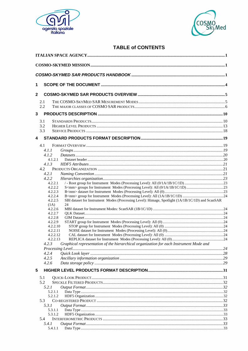
TABLE of CONTENTS ITALIAN SPACE AGENCY...................................................................................................................................1
COSMO-SKYMED MISSION................................................................................................................................1
COSMO-SKYMED SAR PRODUCTS HANDBOOK .........................................................................................1
1 SCOPE OF THE DOCUMENT ......................................................................................................................4
2 COSMO-SKYMED SAR PRODUCTS OVERVIEW ...................................................................................5 2.1 THE COSMO-SKYMED SAR MESUREMENT MODES ..................................................................................5 2.2 THE MAJOR CLASSES OF COSMO SAR PRODUCTS......................................................................................6
3 PRODUCTS DESCRIPTION .......................................................................................................................10 3.1 STANDARDS PRODUCTS.............................................................................................................................10 3.2 HIGHER LEVEL PRODUCTS ........................................................................................................................13 3.3 SERVICE PRODUCTS ..................................................................................................................................18
4 STANDARD PRODUCTS FORMAT DESCRIPTION ..............................................................................19 4.1 FORMAT OVERVIEW..................................................................................................................................19
4.1.1 Groups ..............................................................................................................................................19 4.1.2 Datasets ............................................................................................................................................20
4.1.2.1 Dataset header ...............................................................................................................................................20 4.1.3 HDF5 Attributes ...............................................................................................................................21
4.2 PRODUCTS ORGANIZATION .......................................................................................................................21 4.2.1 Naming Convention ..........................................................................................................................21 4.2.2 Hierarchies organization..................................................................................................................23
4.2.2.1 / - Root group for Instrument Modes (Processing Level): All (0/1A/1B/1C/1D) .........................................23 4.2.2.2 S<mm> groups for Instrument Modes (Processing Level): All (0/1A/1B/1C/1D).......................................23 4.2.2.3 B<nnn> dataset for Instrument Modes (Processing Level): All (0)..............................................................23 4.2.2.4 B<nnn> group for Instrument Modes (Processing Level): All (1A/1B/1C/1D) ...........................................24 4.2.2.5 SBI dataset for Instrument Modes (Processing Level): Himage, Spotlight (1A/1B/1C/1D) and ScanSAR (1A) 24 4.2.2.6 MBI dataset for Instrument Modes: ScanSAR (1B/1C/1D) ..........................................................................24 4.2.2.7 QLK Dataset..................................................................................................................................................24 4.2.2.8 GIM Dataset ..................................................................................................................................................24 4.2.2.9 START group for Instrument Modes (Processing Level): All (0) ................................................................24 4.2.2.10 STOP group for Instrument Modes (Processing Level): All (0) ..............................................................24 4.2.2.11 NOISE dataset for Instrument Modes (Processing Level): All (0)...........................................................24 4.2.2.12 CAL dataset for Instrument Modes (Processing Level): All (0) ..............................................................24 4.2.2.13 REPLICA dataset for Instrument Modes (Processing Level): All (0) ......................................................24
4.2.3 Graphical representation of the hierarchical organization for each Instrument Mode and Processing Level...............................................................................................................................................24 4.2.4 Quick Look layer ..............................................................................................................................28 4.2.5 Ancillary information organization ..................................................................................................29 4.2.6 Data storage policy ..........................................................................................................................29
5 HIGHER LEVEL PRODUCTS FORMAT DESCRIPTION .......................................................................31 5.1 QUICK-LOOK PRODUCT.............................................................................................................................31 5.2 SPECKLE FILTERED PRODUCTS..................................................................................................................32
5.2.1 Output Format ..................................................................................................................................32 5.2.1.1 Data Type ......................................................................................................................................................32 5.2.1.2 HDF5 Organization .......................................................................................................................................32
5.3 CO-REGISTERED PRODUCT ........................................................................................................................32 5.3.1 Output Format ..................................................................................................................................33
5.3.1.1 Data Type ......................................................................................................................................................33 5.3.1.2 HDF5 Organization .......................................................................................................................................33
5.4 INTERFEROMETRIC PRODUCTS ..................................................................................................................33 5.4.1 Output Format ..................................................................................................................................33
5.4.1.1 Data Type ......................................................................................................................................................33
5.4.1.2 HDF5 Organization .......................................................................................................................................33 5.5 DEM PRODUCT .........................................................................................................................................35
5.5.1 Output Format ..................................................................................................................................35 5.5.1.1 Data Type ......................................................................................................................................................35 5.5.1.2 HDF5 Organization .......................................................................................................................................36
5.6 MOSAICKED PRODUCT ..............................................................................................................................36 5.6.1 Output Format ..................................................................................................................................36
5.6.1.1 Data Type ......................................................................................................................................................37 5.6.1.2 HDF5 Organization .......................................................................................................................................37
6 APPENDIX: PRODUCT ATTRIBUTES .....................................................................................................39
7 ACRONYMS AND GLOSSARY................................................................................................................103 7.1 ACRONYMS .............................................................................................................................................103 7.2 GLOSSARY...............................................................................................................................................104

1 Scope of the Document Scope of the Document is to provide COSMO-SkyMed System Users with a SAR Product Handbook giving a quite detailed description of the COSMO SAR Products.
2 COSMO-SkyMed SAR Products Overview This chapter, after a brief summary of the COSMO-SkyMed SAR Measuring Modes, describes the three major classes of COSMO-SkyMed SAR products and the related products tree.
2.1 The COSMO-SkyMed SAR Mesurement Modes
Fig. 1 - COSMO SAR Measurement Modes and related characteristics
The COSMO-SkyMed SAR instrument can be operated in different beam which include:
• Spotlight (mode 2 and mode 1) (Note: mode 1 is for Defence use only and is not further described)
• Stripmap (himage and pingpong) • Scansar (wideregion or hugeregion)
The characteristics of SAR measurement modes are briefly delineated hereafter:
• SPOTLIGHT, allowing SAR images with spot extension of 10.x10. km2 and spatial resolution equal to 1.x1. m2 single look (Spotlight 2);
• STRIPMAP (HIMAGE achieving medium resolution, wide swath imaging, with swath extension ≥40 km and spatial resolution of 3x3 m2 single look;
• STRIPMAP (PINGPONG), achieving medium resolution, medium swath imaging with two radar polarization’s selectable among HH, HV, VH and VV, a spatial resolution of 15 meters on a swath ≥30 km;
• SCANSAR (WIDE and HUGE region), achieving radar imaging with swath extension selectable from 100.x 100. km2 (WIDE REGION) to 200.x 200 km2 (HUGE REGION), and a spatial resolution selectable from 30x30. m2 to 100.x100 m2
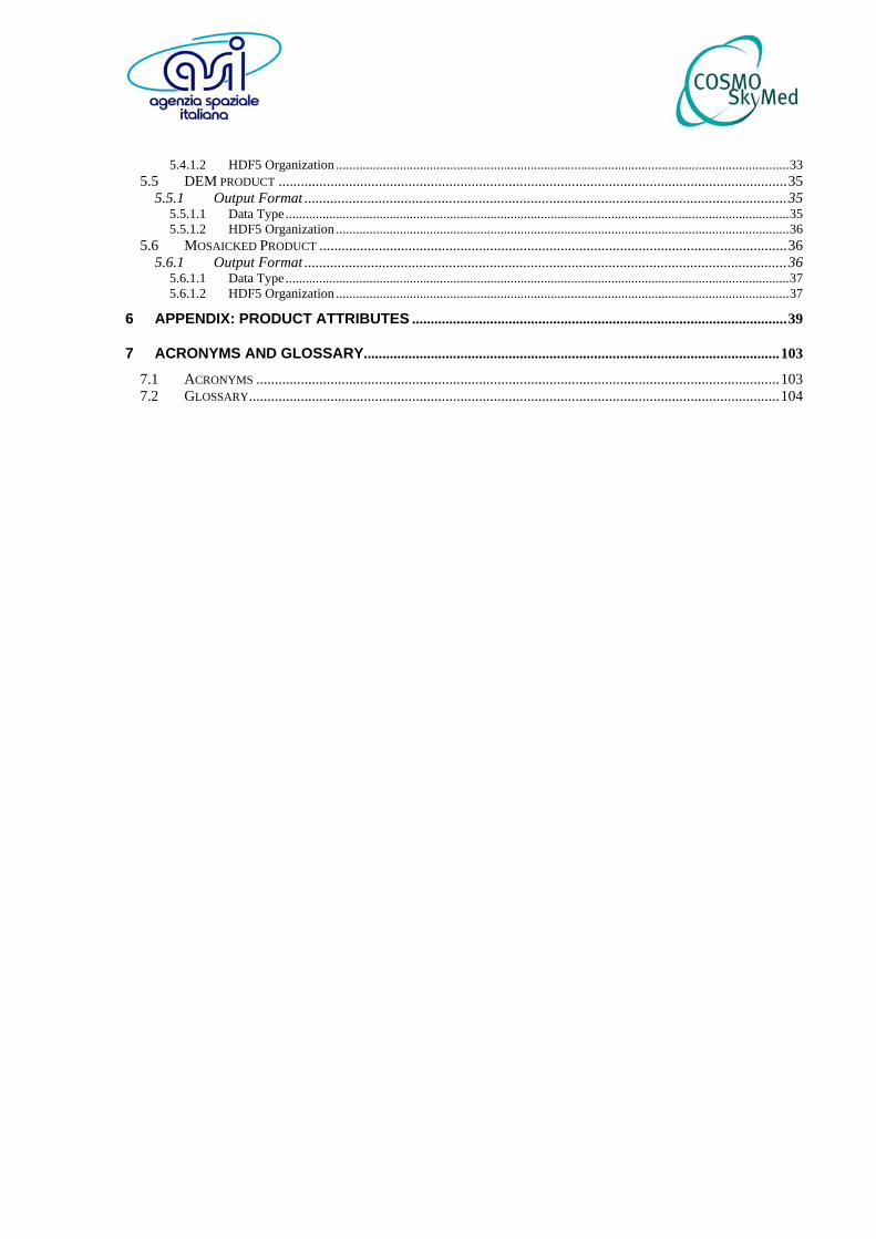
Fig. 2 - Examples of COSMO-SkyMed SAR products The common quality parameters of all the SAR products are:
• PSLR ≤ -22 dB • ISLR ≤ -12 dB • Azimuth Point Target Ambiguity ≤ -40 dB • Radiom. Accuracy ≤ -1 dB (single look) • Radiom. Linearity ≤ -1.5 dB • Radiom. Stability ≤ -1 dB • Total NE°σ ≤ -19 dBm2/m2
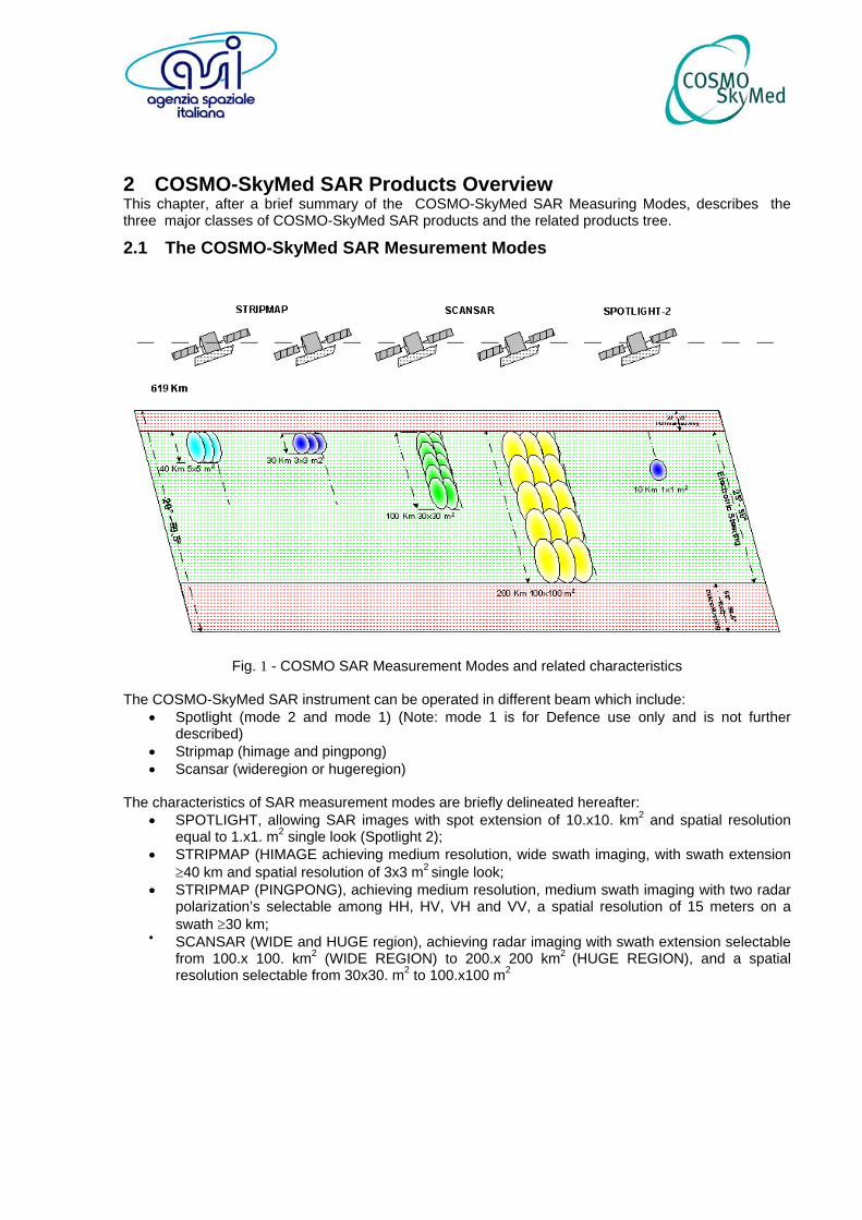
2.2 The major classes of COSMO SAR products The COSMO-SkyMed products are divided in the following major classes:
• Standard products • Higher level products • Service products (for internal use only)
COSMO products
SAR Standard SAR Higher Level Auxiliary products
Fig. 3 – The 3 classes of COSMO-SkyMed products The SAR Standard products are the basic image products of the system, are suitable for many remote sensing applications based on direct usage of low level products and are subdivided into 4 typologies, coded as:
• Level 0 RAW data, defined as “on board raw data (after decryption and before unpacking) associated with auxiliary data including calibration data required to produce higher level products”. This data consists of time ordered echo data, obtained after decryption and decompression (i.e. conversion from BAQ encoded data to 8-bit uniformly quantised data) and after applying internal calibration and error compensation; it include all the auxiliary data (e.g.: trajectography, accurately dated satellite’s co-ordinates and speed vector, geometric sensor model, payload status, calibration data,..) required to produce the other basic and intermediate products.
• 1A, Single-look Complex Slant product, RAW data focused in slant range-azimuth projection, that is the sensor natural acquisition projection; product contains In-Phase and Quadrature of the focused data, weighted and radiometrically equalized
• 1B, Detected Ground Multi-look product, obtained detecting, multi-looking and projecting the
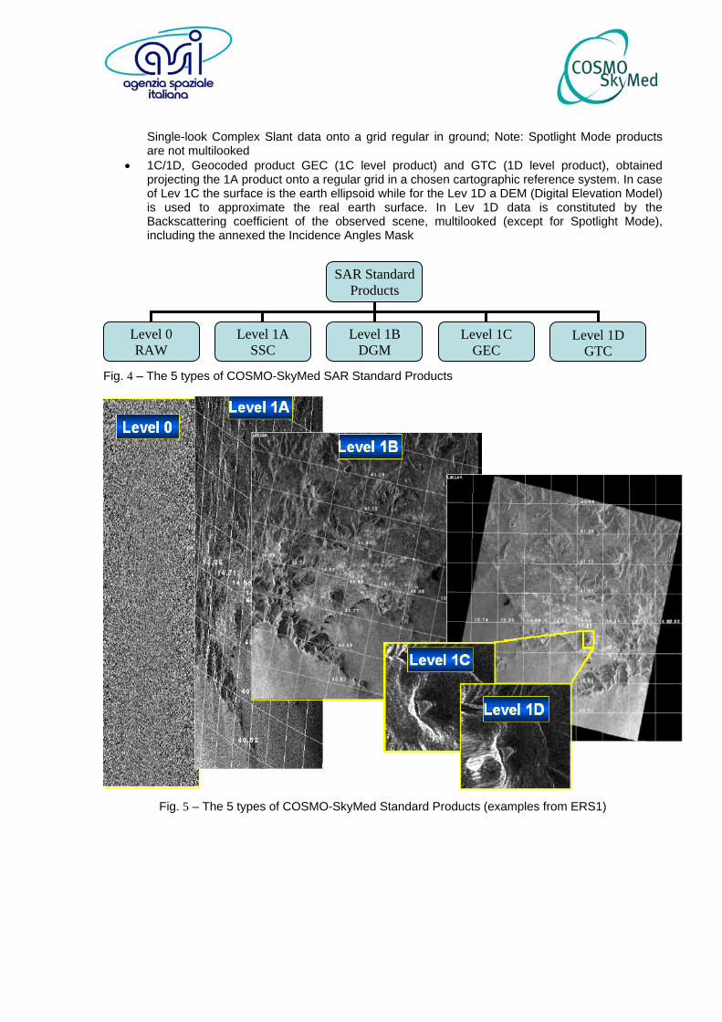
Single-look Complex Slant data onto a grid regular in ground; Note: Spotlight Mode products are not multilooked
• 1C/1D, Geocoded product GEC (1C level product) and GTC (1D level product), obtained projecting the 1A product onto a regular grid in a chosen cartographic reference system. In case of Lev 1C the surface is the earth ellipsoid while for the Lev 1D a DEM (Digital Elevation Model) is used to approximate the real earth surface. In Lev 1D data is constituted by the Backscattering coefficient of the observed scene, multilooked (except for Spotlight Mode), including the annexed the Incidence Angles Mask
SAR StandardProducts
Level 0 RAW
Level 1A SSC
Level 1B DGM
Level 1C GEC
Level 1D GTC
Fig. 4 – The 5 types of COSMO-SkyMed SAR Standard Products
Fig. 5 – The 5 types of COSMO-SkyMed Standard Products (examples from ERS1)
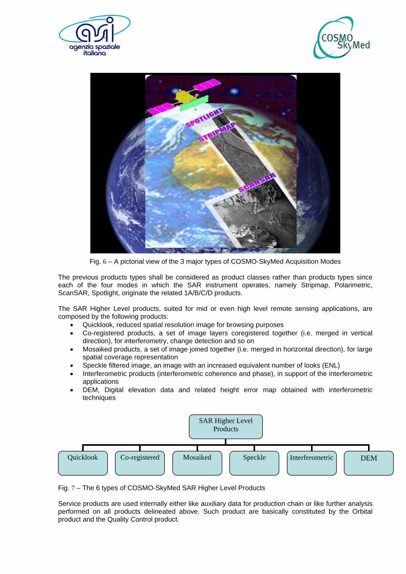
Fig. 6 – A pictorial view of the 3 major types of COSMO-SkyMed Acquisition Modes
The previous products types shall be considered as product classes rather than products types since each of the four modes in which the SAR instrument operates, namely Stripmap, Polarimetric, ScanSAR, Spotlight, originate the related 1A/B/C/D products. The SAR Higher Level products, suited for mid or even high level remote sensing applications, are composed by the following products:
• Quicklook, reduced spatial resolution image for browsing purposes • Co-registered products, a set of image layers coregistered together (i.e. merged in vertical
direction), for interferometry, change detection and so on • Mosaiked products, a set of image joined together (i.e. merged in horizontal direction), for large
spatial coverage representation • Speckle filtered image, an image with an increased equivalent number of looks (ENL) • Interferometric products (interferometric coherence and phase), in support of the interferometric
applications • DEM, Digital elevation data and related height error map obtained with interferometric
techniques
SAR Higher Level Products
Quicklook Co-registered Mosaiked Speckle Interferometric DEM
Fig. 7 – The 6 types of COSMO-SkyMed SAR Higher Level Products Service products are used internally either like auxiliary data for production chain or like further analysis performed on all products delineated above. Such product are basically constituted by the Orbital product and the Quality Control product.
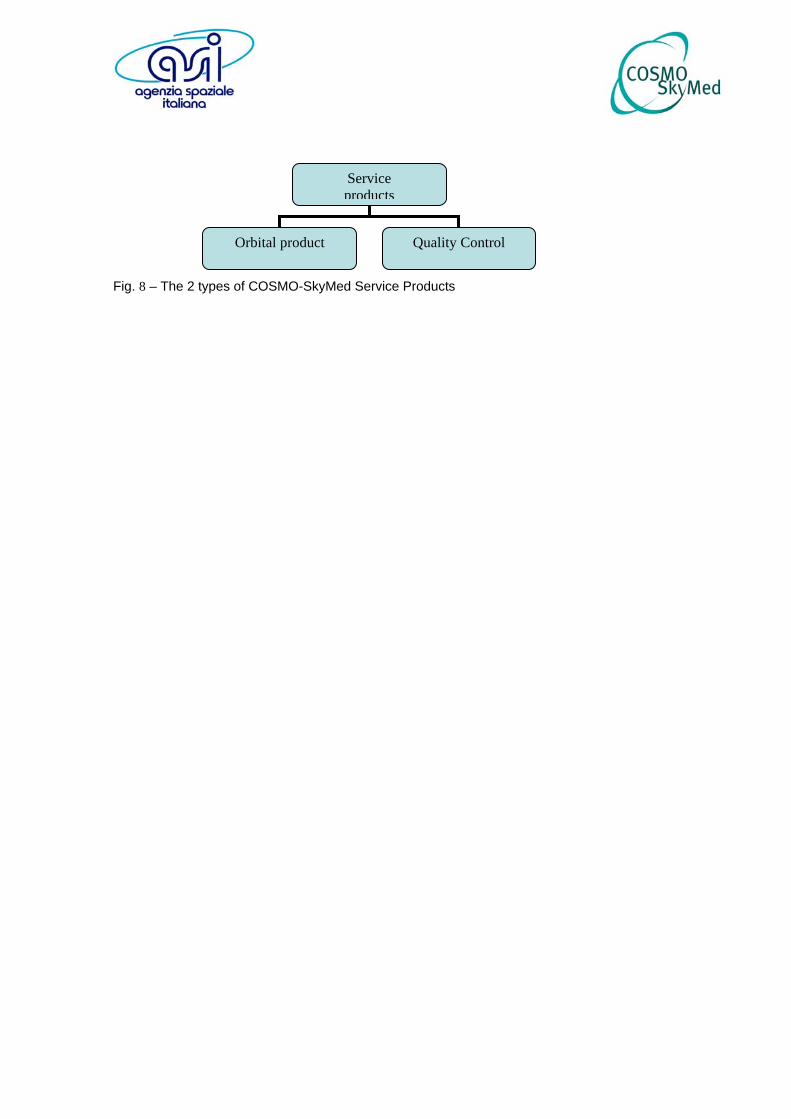
Service products
Orbital product Quality Control
Fig. 8 – The 2 types of COSMO-SkyMed Service Products
3 Products Description The COSMO-SkyMed products are divided in the following major classes and briefly described in next sections:
• Standard products • Higher level products • Service products (for internal use only)
3.1 Standards Products The foreseen standard processing levels (from level 0 up to 1D) are compliant with the definitions given in international standards for Earth Observation (e.g. CEOS guidelines). A further categorization defines the standard processing through three successive stages:
• Pre-processing • Processing • Image geo-localization
Pre-processing stage involves the operations that are normally required prior to the main data analysis and extraction of information (i.e. Level 0 processing). Processing stage mainly performs radiometric and geometric corrections of the imagery (i.e. Level 1A and Level 1B processing). The last thread of this elaboration chain is the projection of the imagery on known reference system (i.e. Level 1C and Level 1D processing). The following standard processing levels are conceived for COSMO:
• Level 0 (RAW), containing for each sensor acquisition mode the unpacked echo data in complex in-phase and quadrature signal (I and Q) format. The processing performed on the down linked X-band raw signal data are:
frame synchronization transmission protocol removal packet data filed re-assembly data decompression statistics estimation data formatting
• Level 1A products (SCS), whose processing is aimed at generating Single-look Complex Slant (SCS) products. The SCS product, obtained after the L1A processing, contains focused data in complex format, in slant range and zero Doppler projection. The processing performed on L0 input data are:
gain receiver compensation internal calibration data focusing statistics estimation of the output data data formatting into output
• Level 1B Products (MDG), whose processing is aimed at generating Detected Ground Multi-look (MDG) products, starting from input (L1A) data. A MDG product, obtained after L1B processing, contains focused data, detected, radiometrically equalized and in ground range/azimuth projection. The processing performed on L1A input data are:
multi-looking for speckle reduction image detection (amplitude) ellipsoid ground projection statistics evaluation data formatting
• Level 1C Products (GEC), whose processing is aimed at generating Geocoded Ellipsoid Corrected (GEC) products. A GEC product, obtained after L1C processing, contains focused data, detected geo-located on the reference ellipsoid and represented in a uniform pre-selected cartographic presentation. The processing performed on L1B input data are:
multi-looking for speckle reduction ellipsoid map projection statistics evaluation data formatting
• Level 1D Products (GTC), whose processing is aimed at generating Geocoded Terrain Corrected (GTC) products. A GTC product, obtained after L1D processing, contains focused data projected onto a reference elevation surface in a regular grid obtained from a cartographic reference system. The image scene is located and accurately (x, y, z) rectified onto a map projection, through the use of Ground Control Points (GCPs) and Digital Elevation Model (DEM). The processing performed on L1B input data is actually GEC processing with the use of the DEM for map projection.
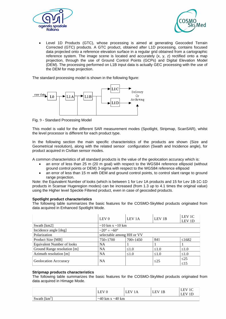
The standard processing model is shown in the following figure:
Fig. 9 - Standard Processing Model This model is valid for the different SAR measurement modes (Spotlight, Stripmap, ScanSAR), whilst the level processor is different for each product type. In the following section the main specific characteristics of the products are shown (Size and Geometrical resolution), along with the related sensor configuration (Swath and Incidence angle), for product acquired in Civilian sensor modes. A common characteristics of all standard products is the value of the geolocation accuracy which is:
• an error of less than 25 m (20 m goal) with respect to the WGS84 reference ellipsoid (without ground control points or DEM) 3-sigma with respect to the WGS84 reference ellipsoid
• an error of less than 15 m with DEM and ground control points, to control slant range to ground range projection.
Note: the Equivalent Number of looks (which is between 1 for Lev 1A products and 15 for Lev 1B-1C-1D products in Scansar Hugeregion modes) can be increased (from 1.3 up to 4.1 times the original value) using the Higher level Speckle Filtered product, even in case of geocoded products. Spotlight product characteristics The following table summarizes the basic features for the COSMO-SkyMed products originated from data acquired in Enhanced Spotlight Mode.
LEV 0 LEV 1A LEV 1B LEV 1C LEV 1D
Swath [km2] ~10 km x ~10 km Incidence angle [deg] ~20° ÷ ~60° Polarization selectable among HH or VV Product Size [MB] 750÷1700 700÷1450 841 ≤1682 Equivalent Number of looks NA 1 1 1 Ground Range resolution [m] NA ≤1.0 ≤1.0 ≤1.0 Azimuth resolution [m] NA ≤1.0 ≤1.0 ≤1.0
Geolocation Acccuracy NA ≤25 ≤25 ≤15
Stripmap products characteristics The following table summarizes the basic features for the COSMO-SkyMed products originated from data acquired in Himage Mode.
LEV 0 LEV 1A LEV 1B LEV 1C LEV 1D
Swath [km2] ~40 km x ~40 km
Incidence angle [deg] ~20° ÷ ~60° Polarization selectable among HH or HV or VH or VV Product Size [MB] 800÷1250 1150÷1800 390÷590 ≤1118 Equivalent Number of looks NA 1 ~ 3 ∼ 3 Ground Range resolution [m] NA ≤3.0 ≤5.0 ≤5.0 Azimuth resolution [m] NA ≤3.0 ≤5.0 ≤5.0
Geolocation Acccuracy NA ≤25 ≤25 ≤15
Polarimetric products characteristics The following table summarizes the basic features for the COSMO-SkyMed products originated from data acquired in PingPong Mode.
LEV 0 LEV 1A LEV 1B LEV 1C LEV 1D
Swath [km2] ~30 km x ~30 km Incidence angle [deg] ~20° ÷ ~60°
Polarization The two polarimetric channels contains: HH,VV or HH,HV or VV,VH
Product Size [MB] 120÷200 430÷650 45÷70 ≤140 Equivalent Number of looks NA 1 ~ 3.7 ~ 3.7 Ground Range resolution [m] NA ≤15.0 ≤20.0 ≤20.0 Azimuth resolution [m] NA ≤15.0 ≤20.0 ≤20.0
Geolocation Acccuracy NA ≤25 ≤25 ≤20
ScanSAR Wideregion products characteristics The following table summarizes the basic features for the COSMO-SkyMed products originated from data acquired in WideRegion Mode.
LEV 0 LEV 1A LEV 1B LEV 1C LEV 1D
Swath [km2] ~100 km x ~100 km Incidence angle [deg] ~20° ÷ ~60° Polarization selectable among HH or HV or VH or VV Product Size [MB] 840÷1100 1300÷1800 85÷150 ≤300 Equivalent Number of looks NA 1 ~ 13 ~ 13 Ground Range resolution [m] NA ≤7.0 ≤30.0 ≤30.0 Azimuth resolution [m] NA ≤16.0 ≤30.0 ≤30.0
Geolocation Acccuracy NA ≤30 ≤30 ≤30
ScanSAR Hugeregion products characteristics The following table summarizes the basic features for the COSMO-SkyMed products originated from data acquired in HugeRegion Mode.
LEV 0 LEV 1A LEV 1B LEV 1C LEV 1D
Swath [km2] ~200 km x ~200 km Incidence angle [deg] ~20° ÷ ~60° Polarization selectable among HH or HV or VH or VV Product Size [MB] 460÷590 580÷730 28÷40 <80 Equivalent Number of looks NA 1 ~ 23 ~ 23 Ground Range resolution [m] NA ≤20.0 ≤100.0 ≤100.0
Azimuth resolution [m] NA ≤30.0 ≤100.0 ≤100.0
Geolocation Acccuracy NA ≤100.0 ≤100.0 ≤100.0
3.2 Higher Level Products Higher Level Product include the following types briefly summarized hereafter:
• Quick-Look Products • Speckle Filtered Products • Co-registered Products • Interferometric Products • Digital Elevation Model (DEM) Products • Mosaicked Products
Two further products exists, but since they are envisaged for Defence Users only, are here only listed and not further described:
• Products for Band Reduction • Defence Applications product
Quick Look Products These products are synoptic of the entire datum allowing a look to the image content in a faster way than the one obtained by processing the image according to the standard algorithms. It is an image easy to visualize: this image shall be easily opened and viewed with conventional image software and self explanatory from the geo-location point of view. The main characteristics of the Quicklook produc are:
• the product is detected • the product it’s ground projected • the product has integer pixels with values scaled in the range 0 - 255 • depending by the look side and orbit pass, the order of the columns or lines within the image is
reversed (with respect the level 0 data) in order present the image in the closest way respect a map
• the product has curves (iso-latitude and iso-longitude) which allow the visualization of the geographic coordinates within the image
The Quick Look Products have a degraded processing bandwidth and so the resolution is consequently scaled. The characteristics of the product in terms of geometric resolution and geometric accuracy are however specified and kept under control, in order to allow the usage of this product (whose primary scope is the image browsing) even in remote sensing applications. In the following table the Quick Look Products characteristics of resolution and geometric accuracy are summarized.
Spotlight Stripmap Polarimetric ScanSar Wideregion
ScanSar Hugeregion
Product Size [MB] 17 20÷30 4÷7 8÷15 4÷7 Ground Range resolution [m] ≤ 50 ≤ 100 ≤ 200 ≤ 300 ≤ 600 Azimuth resolution [m] ≤ 50 ≤ 100 ≤ 200 ≤ 300 ≤ 600 Equivalent Number of looks ≥10 ≥10 ≥10 ≥10 ≥10 Geometric accuracy [m] Case of high qualitry GPS data (Selective Avaiability OFF)
≤ 50 ≤ 60 ≤ 100
Geometric accuracy [m] Case of low qualitry GPS data (Selective Avaiability ON)
≤ 150 ≤ 150 ≤ 150 ≤ 150 ≤ 300
Speckle Filtered Products The Higher Level Speckle Filtered Product deals with the improvement of the radiometric resolution of the SAR images by means of the reduction of the intrinsic multiplicative-like speckle noise. Speckle is a multiplicative noise-like characteristic of coherent imaging systems (such as the SAR), which manifests itself in the image as the apparently random placement of pixels which are noticeably bright or dark. In fact the speckle is a real electromagnetic effect that originates from the constructive or destructive
interference (within a resolution cell) of multiple returns of coherent electromagnetic radiation. The COSMO SkyMed SAR Standard Products described above, provide speckle reduction via multi-looking, which may be not suitable for all potential high-level applications of the COSMO data: classification, feature extraction, change analysis and detection, soil parameters estimations. For that fact, the Speckle Filtering processor tries to cope with any generic application that could benefit of a speckle noise suppression, improving the radiometric resolution of the SAR Standard images thus allowing a better estimation of the radiometric quantities and minimizing, whenever possible, side effects (degradation of the spatial resolution, artefacts, feature alteration). As such, the Speckle Filtered Product is derived by post-processing of the SAR Standard Level 1A or 1B products. The filtered product is formally equivalent to a 1B standard product and may be further processed by the SAR Standard chain. Many types of filters are allowable, beloning to various classes (Non-Adaptive, Adaptive MMSE, Adaptive MAP, Morphological). Speckle filtered products can be generated starting from level 1B products and hence originating a product at same level. The expected increase in the Equivalent Number of Looks for the various allowable filters is shown in next table. Filter Equivalent number of looks increasing factors Mean ≥4.1 Median ≥3.0 Lee ≥4.1 Enhanced Lee (dumping factor = 0.5) ≥4.1
Kuan ≥4.1 Frost (dumping factor = 0.5) ≥2.9
Enhanced Frost (dumping factor = 0.5) ≥4.1
Gamma MAP ≥3.7 Crimmins (iteration = 8) ≥1.3
The following table shows the geometric resolution of the speckle filtered products obtained applying a filter having a kenel size of 5 x 5 to 1B products, in the various acquisition modes. Note that the 1B speckle filtered product can be used for the geocoded (Lev 1C-1D) products generation, hence originating speckle filtered geocoded products.
Spotlight Stripmap Polarimetric ScanSar Wideregion
ScanSar Hugeregion
Product Size [MB] same as input Ground Range resolution [m] Azimuth resolution [m] ≤4.5 ≤25.0 ≤90.0 ≤140.0 ≤460.0
Co-registered Products Two different images covering the same area can be made superimposable by means of the co-registration which is the process of lining-up two images, one “master” and the other one is the “slave” image, such to fit exactly on top of each other without adding artifacts in image intensity and phase components. The input images are co-registered using the master as reference. Co-registered images can be taken from simultaneous illuminations of the same scene at different frequencies (multi frequency images), from acquisitions taken at different time using different sensors, from multiple passages of the same satellite (multi temporal images). In general, images have different geometry, thus to be superposed the slave image must be re-sampled into the master geometry. The images may be fully or only partly overlapped and even more than two images can be co-registered at the same time. The co-registration process generates as many output images as the input are: one master image and multiple slave images in input give one co-registered master image and the multiple co-registered slave images. The type of the images is preserved: input real or complex images produce output real or complex co-registered images respectively. As such, the higher level Co-registration products are derived in any acquisition mode, by post-processing of the SAR Level 1A (complex images) or level 1B (real images) SAR standard products, respectively generating a product complex or real (co-registered product). Co-registered products can be further processed by the SAR standard processing chain. The
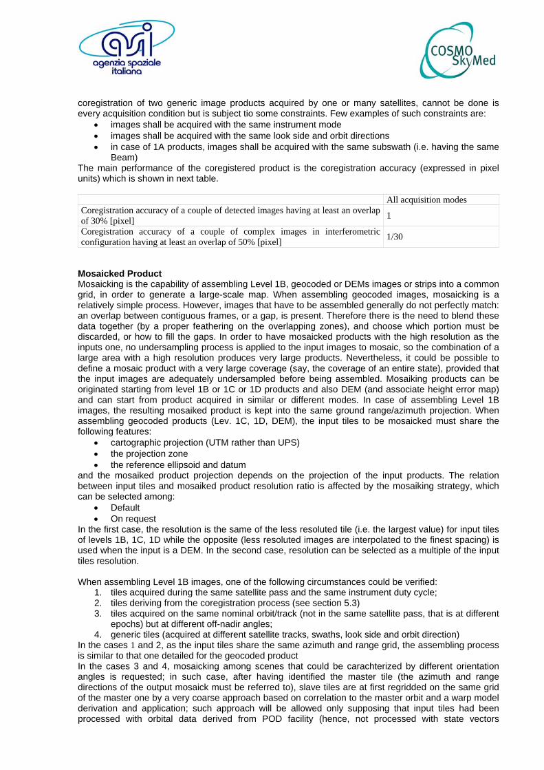
coregistration of two generic image products acquired by one or many satellites, cannot be done is every acquisition condition but is subject tio some constraints. Few examples of such constraints are:
• images shall be acquired with the same instrument mode • images shall be acquired with the same look side and orbit directions • in case of 1A products, images shall be acquired with the same subswath (i.e. having the same
Beam) The main performance of the coregistered product is the coregistration accuracy (expressed in pixel units) which is shown in next table. All acquisition modes Coregistration accuracy of a couple of detected images having at least an overlap of 30% [pixel] 1
Coregistration accuracy of a couple of complex images in interferometric configuration having at least an overlap of 50% [pixel] 1/30
Mosaicked Product Mosaicking is the capability of assembling Level 1B, geocoded or DEMs images or strips into a common grid, in order to generate a large-scale map. When assembling geocoded images, mosaicking is a relatively simple process. However, images that have to be assembled generally do not perfectly match: an overlap between contiguous frames, or a gap, is present. Therefore there is the need to blend these data together (by a proper feathering on the overlapping zones), and choose which portion must be discarded, or how to fill the gaps. In order to have mosaicked products with the high resolution as the inputs one, no undersampling process is applied to the input images to mosaic, so the combination of a large area with a high resolution produces very large products. Nevertheless, it could be possible to define a mosaic product with a very large coverage (say, the coverage of an entire state), provided that the input images are adequately undersampled before being assembled. Mosaiking products can be originated starting from level 1B or 1C or 1D products and also DEM (and associate height error map) and can start from product acquired in similar or different modes. In case of assembling Level 1B images, the resulting mosaiked product is kept into the same ground range/azimuth projection. When assembling geocoded products (Lev. 1C, 1D, DEM), the input tiles to be mosaicked must share the following features:
• cartographic projection (UTM rather than UPS) • the projection zone • the reference ellipsoid and datum
and the mosaiked product projection depends on the projection of the input products. The relation between input tiles and mosaiked product resolution ratio is affected by the mosaiking strategy, which can be selected among:
• Default • On request
In the first case, the resolution is the same of the less resoluted tile (i.e. the largest value) for input tiles of levels 1B, 1C, 1D while the opposite (less resoluted images are interpolated to the finest spacing) is used when the input is a DEM. In the second case, resolution can be selected as a multiple of the input tiles resolution. When assembling Level 1B images, one of the following circumstances could be verified:
1. tiles acquired during the same satellite pass and the same instrument duty cycle; 2. tiles deriving from the coregistration process (see section 5.3) 3. tiles acquired on the same nominal orbit/track (not in the same satellite pass, that is at different
epochs) but at different off-nadir angles; 4. generic tiles (acquired at different satellite tracks, swaths, look side and orbit direction)
In the cases 1 and 2, as the input tiles share the same azimuth and range grid, the assembling process is similar to that one detailed for the geocoded product In the cases 3 and 4, mosaicking among scenes that could be carachterized by different orientation angles is requested; in such case, after having identified the master tile (the azimuth and range directions of the output mosaick must be referred to), slave tiles are at first regridded on the same grid of the master one by a very coarse approach based on correlation to the master orbit and a warp model derivation and application; such approach will be allowed only supposing that input tiles had been processed with orbital data derived from POD facility (hence, not processed with state vectors
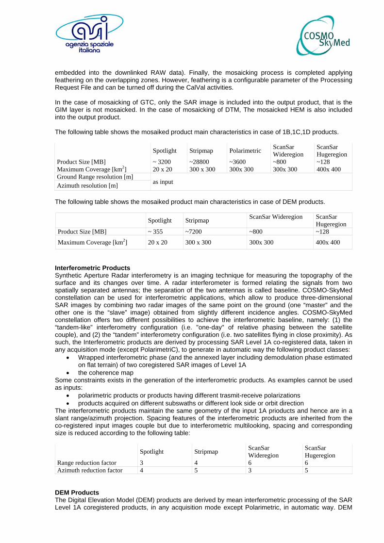
embedded into the downlinked RAW data). Finally, the mosaicking process is completed applying feathering on the overlapping zones. However, feathering is a configurable parameter of the Processing Request File and can be turned off during the CalVal activities. In the case of mosaicking of GTC, only the SAR image is included into the output product, that is the GIM layer is not mosaicked. In the case of mosaicking of DTM, The mosaicked HEM is also included into the output product. The following table shows the mosaiked product main characteristics in case of 1B,1C,1D products.
Spotlight Stripmap Polarimetric ScanSar Wideregion
ScanSar Hugeregion
Product Size [MB] ~ 3200 ~28800 ~3600 ~800 ~128 Maximum Coverage [km2] 20 x 20 300 x 300 300x 300 300x 300 400x 400 Ground Range resolution [m] Azimuth resolution [m] as input
The following table shows the mosaiked product main characteristics in case of DEM products.
Spotlight Stripmap ScanSar Wideregion ScanSar Hugeregion
Product Size [MB] ~ 355 ~7200 ~800 ~128
Maximum Coverage [km2] 20 x 20 300 x 300 300x 300 400x 400
Interferometric Products Synthetic Aperture Radar interferometry is an imaging technique for measuring the topography of the surface and its changes over time. A radar interferometer is formed relating the signals from two spatially separated antennas; the separation of the two antennas is called baseline. COSMO-SkyMed constellation can be used for interferometric applications, which allow to produce three-dimensional SAR images by combining two radar images of the same point on the ground (one “master” and the other one is the “slave” image) obtained from slightly different incidence angles. COSMO-SkyMed constellation offers two different possibilities to achieve the interferometric baseline, namely: (1) the “tandem-like” interferometry configuration (i.e. "one-day" of relative phasing between the satellite couple), and (2) the “tandem” interferometry configuration (i.e. two satellites flying in close proximity). As such, the Interferometric products are derived by processing SAR Level 1A co-registered data, taken in any acquisition mode (except PolarimetriC), to generate in automatic way the following product classes:
• Wrapped interferometric phase (and the annexed layer including demodulation phase estimated on flat terrain) of two coregistered SAR images of Level 1A
• the coherence map Some constraints exists in the generation of the interferometric products. As examples cannot be used as inputs:
• polarimetric products or products having different trasmit-receive polarizations • products acquired on different subswaths or different look side or orbit direction
The interferometric products maintain the same geometry of the input 1A prioducts and hence are in a slant range/azimuth projection. Spacing features of the interferometric products are inherited from the co-registered input images couple but due to interferometric multilooking, spacing and corresponding size is reduced according to the following table:
Spotlight Stripmap ScanSar Wideregion
ScanSar Hugeregion
Range reduction factor 3 4 6 6 Azimuth reduction factor 4 5 3 5
DEM Products The Digital Elevation Model (DEM) products are derived by mean interferometric processing of the SAR Level 1A coregistered products, in any acquisition mode except Polarimetric, in automatic way. DEM
products consist of the ellipsoidal height map and the associated height error map. The attributes defining the DEM products are derived from the SAR image couple, with some substantial changes (e.g. due to the change of the image projection). The DEM product is presented in UTM/UPS cartographic coordinate system respect to WGS84 ellipsoid, different from the input geometry (slant-range). The product is composed by:
• ellipsoidal height map • associated height error map
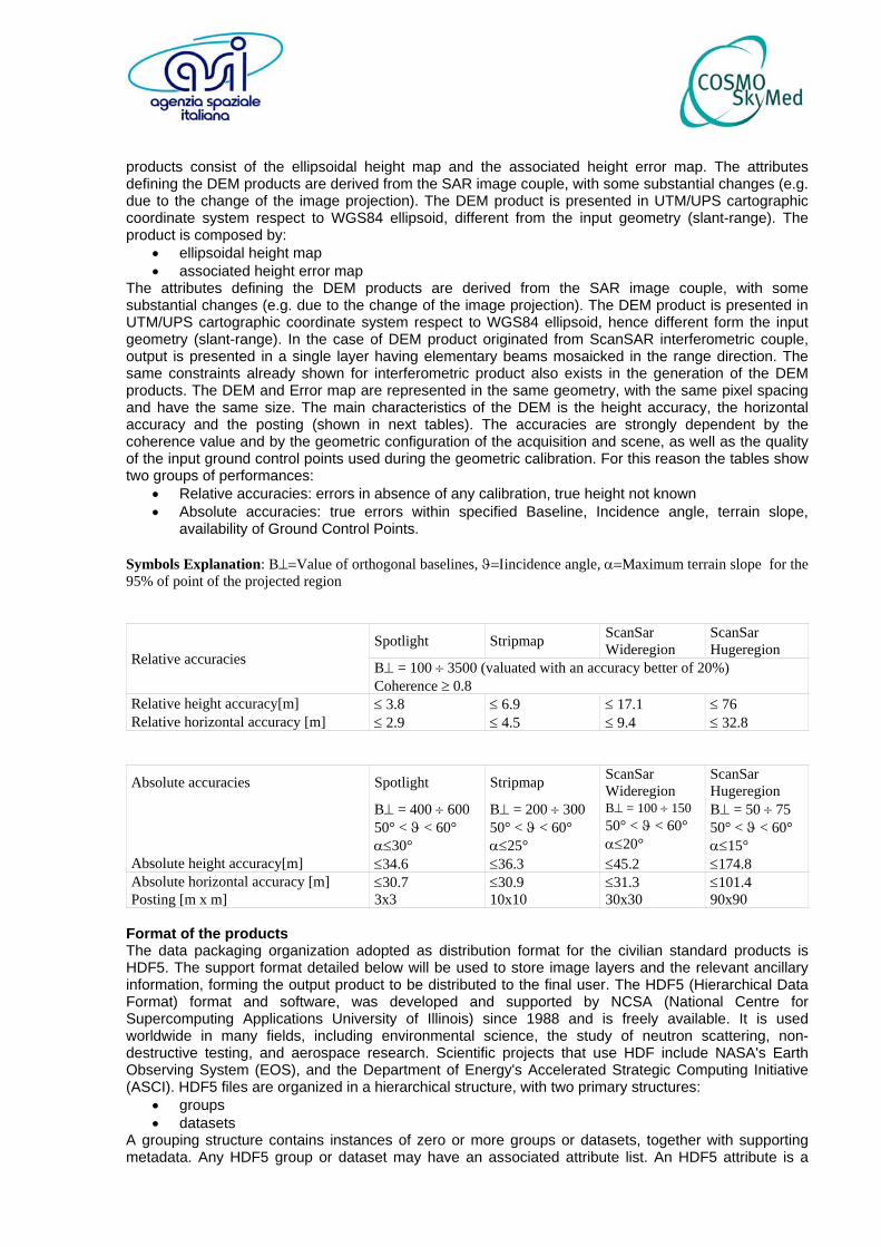
The attributes defining the DEM products are derived from the SAR image couple, with some substantial changes (e.g. due to the change of the image projection). The DEM product is presented in UTM/UPS cartographic coordinate system respect to WGS84 ellipsoid, hence different form the input geometry (slant-range). In the case of DEM product originated from ScanSAR interferometric couple, output is presented in a single layer having elementary beams mosaicked in the range direction. The same constraints already shown for interferometric product also exists in the generation of the DEM products. The DEM and Error map are represented in the same geometry, with the same pixel spacing and have the same size. The main characteristics of the DEM is the height accuracy, the horizontal accuracy and the posting (shown in next tables). The accuracies are strongly dependent by the coherence value and by the geometric configuration of the acquisition and scene, as well as the quality of the input ground control points used during the geometric calibration. For this reason the tables show two groups of performances:
• Relative accuracies: errors in absence of any calibration, true height not known • Absolute accuracies: true errors within specified Baseline, Incidence angle, terrain slope,
availability of Ground Control Points. Symbols Explanation: B⊥=Value of orthogonal baselines, ϑ=Ιincidence angle, α=Maximum terrain slope for the 95% of point of the projected region
Spotlight Stripmap ScanSar Wideregion
ScanSar Hugeregion Relative accuracies B⊥ = 100 ÷ 3500 (valuated with an accuracy better of 20%)
Coherence ≥ 0.8 Relative height accuracy[m] ≤ 3.8 ≤ 6.9 ≤ 17.1 ≤ 76 Relative horizontal accuracy [m] ≤ 2.9 ≤ 4.5 ≤ 9.4 ≤ 32.8
Absolute accuracies Spotlight Stripmap ScanSar Wideregion
ScanSar Hugeregion
B⊥ = 400 ÷ 600 50° < ϑ < 60° α≤30°
B⊥ = 200 ÷ 300 50° < ϑ < 60° α≤25°
B⊥ = 100 ÷ 150 50° < ϑ < 60° α≤20°
B⊥ = 50 ÷ 75 50° < ϑ < 60° α≤15°
Absolute height accuracy[m] ≤34.6 ≤36.3 ≤45.2 ≤174.8 Absolute horizontal accuracy [m] ≤30.7 ≤30.9 ≤31.3 ≤101.4 Posting [m x m] 3x3 10x10 30x30 90x90
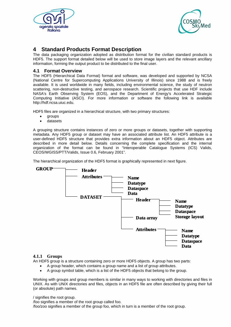
Format of the products The data packaging organization adopted as distribution format for the civilian standard products is HDF5. The support format detailed below will be used to store image layers and the relevant ancillary information, forming the output product to be distributed to the final user. The HDF5 (Hierarchical Data Format) format and software, was developed and supported by NCSA (National Centre for Supercomputing Applications University of Illinois) since 1988 and is freely available. It is used worldwide in many fields, including environmental science, the study of neutron scattering, non-destructive testing, and aerospace research. Scientific projects that use HDF include NASA's Earth Observing System (EOS), and the Department of Energy's Accelerated Strategic Computing Initiative (ASCI). HDF5 files are organized in a hierarchical structure, with two primary structures:
• groups • datasets
A grouping structure contains instances of zero or more groups or datasets, together with supporting metadata. Any HDF5 group or dataset may have an associated attribute list. An HDF5 attribute is a
user-defined HDF5 structure that provides extra information about an HDF5 object. Attributes are described in more detail below. Distribution Media Besides the digital format of the products, the following media types will be used for non-electronic product distribution: DVD, CDROM, Magnetic cassette. Electronic distribution will be based on a FTP access to the COSMO site.
3.3 Service Products The Service Products (only foreseen for internal use) are:
• Orbital product: necessary to perform SAR images geo-location. These products are qualified for several accuracy and latency features according to given processing procedures and ancillary input data
• Quality Control product: necessary to assess the quality of SAR imagery generated by standard- and non-standard processors. The Quality Control (QC) function is able to elaborate products by its own, in order to visualize them and to perform temporal evolution analysis and cross correlation studies. Furthermore, the QC function takes into account the ancillary data, for example the COSMO Orbital Product for the orbital residual trend analysis, and exploits support data (GCP/GRP, DEM, etc) coming from external sources (entities).
4 Standard Products Format Description The data packaging organization adopted as distribution format for the civilian standard products is HDF5. The support format detailed below will be used to store image layers and the relevant ancillary information, forming the output product to be distributed to the final user.
4.1 Format Overview The HDF5 (Hierarchical Data Format) format and software, was developed and supported by NCSA (National Centre for Supercomputing Applications University of Illinois) since 1988 and is freely available. It is used worldwide in many fields, including environmental science, the study of neutron scattering, non-destructive testing, and aerospace research. Scientific projects that use HDF include NASA's Earth Observing System (EOS), and the Department of Energy's Accelerated Strategic Computing Initiative (ASCI). For more information or software the following link is available http://hdf.ncsa.uiuc.edu. HDF5 files are organized in a hierarchical structure, with two primary structures:
• groups • datasets
A grouping structure contains instances of zero or more groups or datasets, together with supporting metadata. Any HDF5 group or dataset may have an associated attribute list. An HDF5 attribute is a user-defined HDF5 structure that provides extra information about an HDF5 object. Attributes are described in more detail below. Details concerning the complete specification and the internal organization of the format can be found in “Interoperable Catalogue Systems (ICS) Valids, CEOS/WGISS/PTT/Valids, Issue 0.6, February 2001”. The hierarchical organization of the HDF5 format is graphically represented in next figure.
GROUP
DATASET
HeaderAttributes Name
DataHeader Name
DatatypeDataspaceStorage layoutData array
DatatypeDataspace
Attributes Name
Data
DatatypeDataspace
GROUP
DATASET
HeaderAttributes Name
DataHeader Name
DatatypeDataspaceStorage layoutData array
DatatypeDataspace
Attributes Name
Data
DatatypeDataspace
4.1.1 Groups An HDF5 group is a structure containing zero or more HDF5 objects. A group has two parts:
• A group header, which contains a group name and a list of group attributes. • A group symbol table, which is a list of the HDF5 objects that belong to the group.
Working with groups and group members is similar in many ways to working with directories and files in UNIX. As with UNIX directories and files, objects in an HDF5 file are often described by giving their full (or absolute) path names. / signifies the root group. /foo signifies a member of the root group called foo. /foo/zoo signifies a member of the group foo, which in turn is a member of the root group.

4.1.2 Datasets A dataset is a multidimensional array of data elements, together with supporting metadata. A dataset is stored in a file in two parts
• A header • A data array
4.1.2.1 Dataset header The header contains information that is needed to interpret the array portion of the dataset, as well as metadata (or pointers to metadata) that describes or annotates the dataset. Header information includes the name of the object, its dimensionality, its number-type, information about how the data itself is stored on disk, and other information used by the library to speed up access to the dataset or maintain the file's integrity. There are four essential classes of information in any header:
• Name • Datatype • Dataspace • Storage layout
4.1.2.1.1 Name A dataset name is a sequence of alphanumeric ASCII characters. 4.1.2.1.2 Datatype HDF5 allows one to define many different kinds of datatypes. There are two categories of datatypes:
• atomic datatypes (which differentiates in system-specific, NATIVE or named) • compound datatypes (which can only be named).
Atomic datatypes are those that are not decomposed at the datatype interface level, such as integers and floats. NATIVE datatypes are system-specific instances of atomic datatypes. Compound datatypes are made up of atomic datatypes. Named datatypes are either atomic or compound datatypes that have been specifically designated to be shared across datasets. Atomic datatypes include integers and floating-point numbers. Each atomic type belongs to a particular class and has several properties: size, order, precision, and offset. In this introduction, we consider only a few of these properties. Atomic classes include integer, float, date and time, string, bit field, and opaque. (Note: Only integer, float and string classes are available in the current implementation.) Properties of integer types include size, order (endian-ness), and signed-ness (signed/unsigned). Properties of float types include the size and location of the exponent and mantissa, and the location of the sign bit. The datatypes that are supported in the current implementation are:
• Integer datatypes: 8-bit, 16-bit, 32-bit, and 64-bit integers in both little and big-endian format. • Floating-point numbers: IEEE 32-bit and 64-bit floating-point numbers in both little and big-
endian format • References • Strings • NATIVE datatypes. Although it is possible to describe nearly any kind of atomic data type, most
applications will use predefined datatypes that are supported by their compiler. In HDF5 these are called native datatypes. NATIVE datatypes are C-like datatypes that are generally supported by the hardware of the machine on which the library was compiled. In order to be portable, applications should almost always use the NATIVE designation to describe data values in memory.
The NATIVE architecture has base names that do not follow the same rules as the others. Instead, native type names are similar to the C type names. A compound datatype is one in which a collection of simple datatypes are represented as a single unit, similar to a struct in C. The parts of a compound datatype are called members. The members of a compound datatype may be of any datatype, including another compound datatype. It is possible to read members from a compound type without reading the

whole type. Named datatypes. Normally each dataset has its own datatype, but sometimes we may want to share a datatype among several datasets. This can be done using a named datatype. A named data type is stored in the file independently of any dataset, and referenced by all datasets that have that datatype. Named datatypes may have an associated attributes list. See Datatypes in the HDF User’s Guide for further information. 4.1.2.1.3 Dataspace A dataset dataspace describes the dimensionality of the dataset. The dimensions of a dataset can be fixed (unchanging), or they may be unlimited, which means that they are extendible (i.e. they can grow larger). Properties of a dataspace consist of the rank (number of dimensions) of the data array, the actual sizes of the dimensions of the array, and the maximum sizes of the dimensions of the array. For a fixed-dimension dataset, the actual size is the same as the maximum size of a dimension. A dataspace can also describe portions of a dataset, making it possible to do partial I/O operations on selections. Given an n-dimensional dataset, there are currently four ways to do partial selection:
• Select a logically contiguous n-dimensional hyperslab. • Select a non-contiguous hyperslab consisting of elements or blocks of elements (hyperslabs)
that are equally spaced. • Select a union of hyperslabs. • Select a list of independent points.
Since I/O operations have two end-points, the raw data transfer functions require two dataspace arguments: one describes the application memory dataspace or subset thereof, and the other describes the file dataspace or subset thereof. 4.1.2.1.4 Storage layout The HDF5 format makes it possible to store data in a variety of ways. The default storage layout format is contiguous, meaning that data is stored in the same linear way that it is organized in memory. Two other storage layout formats are currently defined for HDF5: compact, and chunked. In the future, other storage layouts may be added. Compact storage is used when the amount of data is small and can be stored directly in the object header. Chunked storage involves dividing the dataset into equal-sized "chunks" that are stored separately. Chunking has three important benefits. It makes it possible to achieve good performance when accessing subsets of the datasets, even when the subset to be chosen is orthogonal to the normal storage order of the dataset. It makes it possible to compress large datasets and still achieve good performance when accessing subsets of the dataset. It makes it possible efficiently to extend the dimensions of a dataset in any direction.
4.1.3 HDF5 Attributes Attributes are small named datasets that can be attached to one of the following structures:
• primary datasets • groups • named datatypes
Attributes can be used to describe the nature and/or the intended usage of a dataset or group. An attribute has two parts:
• name • value
The value part contains one or more data entries of the same data type. When accessing attributes, they can be identified by name or by an index value. The use of an index value makes it possible to iterate through all of the attributes associated with a given object.
4.2 Products Organization Specific data organization will be detailed to meet the storage needs of data acquired with all the instrument modes allowed by the COSMO-SkyMed constellation.
4.2.1 Naming Convention The following naming convention will be used for the identification of the COSMO-SkyMed SAR Standard Products files and the most of the Higher Level Products files. Differences in the convention used for some Higher-Level product is detailed into the specific subsection
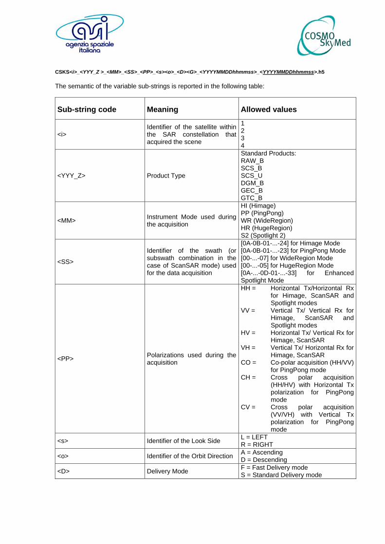
CSKS<i>_<YYY_Z >_<MM>_<SS>_<PP>_<s><o>_<D><G>_<YYYYMMDDhhmmss>_<YYYYMMDDhhmmss>.h5 The semantic of the variable sub-strings is reported in the following table:
Sub-string code Meaning Allowed values
<i> Identifier of the satellite within the SAR constellation that acquired the scene
1 2 3 4
<YYY_Z> Product Type
Standard Products: RAW_B SCS_B SCS_U DGM_B GEC_B GTC_B
<MM> Instrument Mode used during the acquisition
HI (Himage) PP (PingPong) WR (WideRegion) HR (HugeRegion) S2 (Spotlight 2)
<SS>
Identifier of the swath (or subswath combination in the case of ScanSAR mode) used for the data acquisition
[0A-0B-01-...-24] for Himage Mode [0A-0B-01-...-23] for PingPong Mode [00-...-07] for WideRegion Mode [00-...-05] for HugeRegion Mode [0A-...-0D-01-...-33] for Enhanced Spotlight Mode
<PP> Polarizations used during the acquisition
HH = Horizontal Tx/Horizontal Rx for Himage, ScanSAR and Spotlight modes
VV = Vertical Tx/ Vertical Rx for Himage, ScanSAR and Spotlight modes
HV = Horizontal Tx/ Vertical Rx for Himage, ScanSAR
VH = Vertical Tx/ Horizontal Rx for Himage, ScanSAR
CO = Co-polar acquisition (HH/VV) for PingPong mode
CH = Cross polar acquisition (HH/HV) with Horizontal Tx polarization for PingPong mode
CV = Cross polar acquisition (VV/VH) with Vertical Tx polarization for PingPong mode
<s> Identifier of the Look Side L = LEFT R = RIGHT
<o> Identifier of the Orbit Direction A = Ascending D = Descending
<D> Delivery Mode F = Fast Delivery mode S = Standard Delivery mode
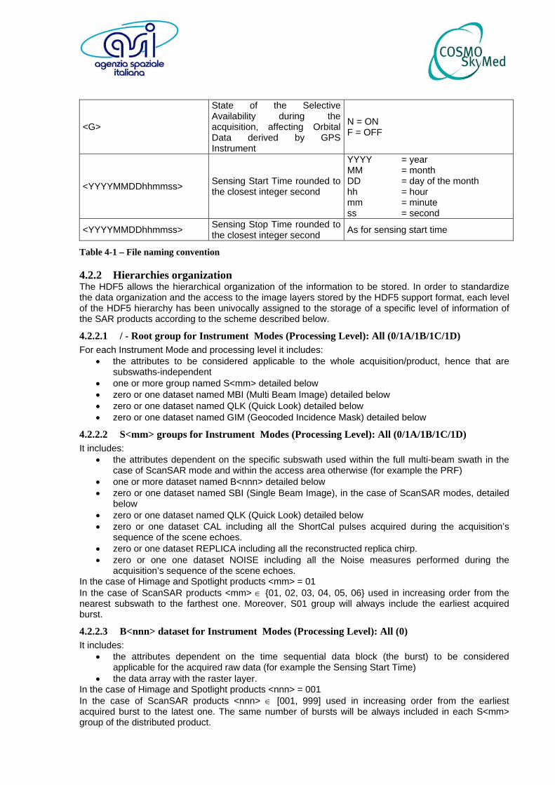
<G>
State of the Selective Availability during the acquisition, affecting Orbital Data derived by GPS Instrument
N = ON F = OFF
<YYYYMMDDhhmmss> Sensing Start Time rounded to the closest integer second
YYYY = year MM = month DD = day of the month hh = hour mm = minute ss = second
<YYYYMMDDhhmmss> Sensing Stop Time rounded to the closest integer second As for sensing start time
Table 4-1 – File naming convention
4.2.2 Hierarchies organization The HDF5 allows the hierarchical organization of the information to be stored. In order to standardize the data organization and the access to the image layers stored by the HDF5 support format, each level of the HDF5 hierarchy has been univocally assigned to the storage of a specific level of information of the SAR products according to the scheme described below.
4.2.2.1 / - Root group for Instrument Modes (Processing Level): All (0/1A/1B/1C/1D) For each Instrument Mode and processing level it includes:
• the attributes to be considered applicable to the whole acquisition/product, hence that are subswaths-independent
• one or more group named S<mm> detailed below • zero or one dataset named MBI (Multi Beam Image) detailed below • zero or one dataset named QLK (Quick Look) detailed below • zero or one dataset named GIM (Geocoded Incidence Mask) detailed below
4.2.2.2 S<mm> groups for Instrument Modes (Processing Level): All (0/1A/1B/1C/1D) It includes:
• the attributes dependent on the specific subswath used within the full multi-beam swath in the case of ScanSAR mode and within the access area otherwise (for example the PRF)
• one or more dataset named B<nnn> detailed below • zero or one dataset named SBI (Single Beam Image), in the case of ScanSAR modes, detailed
below • zero or one dataset named QLK (Quick Look) detailed below • zero or one dataset CAL including all the ShortCal pulses acquired during the acquisition’s
sequence of the scene echoes. • zero or one dataset REPLICA including all the reconstructed replica chirp. • zero or one one dataset NOISE including all the Noise measures performed during the
acquisition’s sequence of the scene echoes. In the case of Himage and Spotlight products <mm> = 01 In the case of ScanSAR products <mm> ∈ {01, 02, 03, 04, 05, 06} used in increasing order from the nearest subswath to the farthest one. Moreover, S01 group will always include the earliest acquired burst.
4.2.2.3 B<nnn> dataset for Instrument Modes (Processing Level): All (0) It includes:
• the attributes dependent on the time sequential data block (the burst) to be considered applicable for the acquired raw data (for example the Sensing Start Time)
• the data array with the raster layer. In the case of Himage and Spotlight products <nnn> = 001 In the case of ScanSAR products <nnn> ∈ [001, 999] used in increasing order from the earliest acquired burst to the latest one. The same number of bursts will be always included in each S<mm> group of the distributed product.
4.2.2.4 B<nnn> group for Instrument Modes (Processing Level): All (1A/1B/1C/1D) It includes the attributes dependent on the time sequential data block (the burst) to be considered applicable for the acquired raw data (for example the Sensing Start Time)
4.2.2.5 SBI dataset for Instrument Modes (Processing Level): Himage, Spotlight (1A/1B/1C/1D) and ScanSAR (1A)
It includes: • the attributes dependent on the subswath used within the access area to be considered
applicable for the distributed product (for example the Line Time Interval) • one raster data array representing the product to be distributed
4.2.2.6 MBI dataset for Instrument Modes: ScanSAR (1B/1C/1D) It includes
• the attributes dependent on the mosaicked full scene to be considered applicable for the distributed product (for example the Line Time Interval)
• one raster data array representing the range/azimuth mosaicked product to be distributed
4.2.2.7 QLK Dataset It includes the quick look of the distributed product. See 4.2.4 for further details.
4.2.2.8 GIM Dataset It includes the raster layer representing the mask (coregistered with the GTC product) of the incidence angles at which each pixel included into the level 1D product had been acquired.
4.2.2.9 START group for Instrument Modes (Processing Level): All (0) It includes the dataset of Calibration (CAL) and Noise (NOISE) measurements performed during the acquisition initialization sequence extracted from the downlinked RAW data
4.2.2.10 STOP group for Instrument Modes (Processing Level): All (0) It includes the dataset of Calibration (CAL) and Noise (NOISE) measurements performed during the acquisition termination sequence extracted from the downlinked RAW data
4.2.2.11 NOISE dataset for Instrument Modes (Processing Level): All (0) It includes the Noise data from the downlinked RAW data.
• The dataset START/NOISE (respectively STOP/NOISE), includes the Noise measurements performed during the acquisition Initialization (respectively Termination) sequence;
• The dataset /S<nn>/NOISE, includes all the Noise measures performed during the acquisition’s sequence of the scene echoes
4.2.2.12 CAL dataset for Instrument Modes (Processing Level): All (0) It includes the Calibration data from the downlinked RAW data. Three cases can be identified:
• the dataset /START/CAL, includes all the Calibration measurements (Tx1a, Tx1b and Rx performed on each row of the antenna plus an additional ShortCal pulse) performed during the acquisition’s Initialization sequence;
• the dataset /STOP/CAL, includes all the Calibration measurements (Tx1a, Tx1b and Rx performed on each row of the antenna plus an additional ShortCal pulse) performed during the acquisition’s Termination sequence;
• the dataset /S<nn>/CAL, includes all the ShortCal pulses acquired during the acquisition’s sequence of the scene echoes.
4.2.2.13 REPLICA dataset for Instrument Modes (Processing Level): All (0) It includes the replica chirp reconstructed from the calibration data included into the downlinked RAW data. It includes a number of lines equal to the number of measured ShortCal pulses
4.2.3 Graphical representation of the hierarchical organization for each Instrument Mode and Processing Level
The hierarchical organization for each Instrument Mode and Processing Level is graphically represented in the following diagrams A not colour filled structure
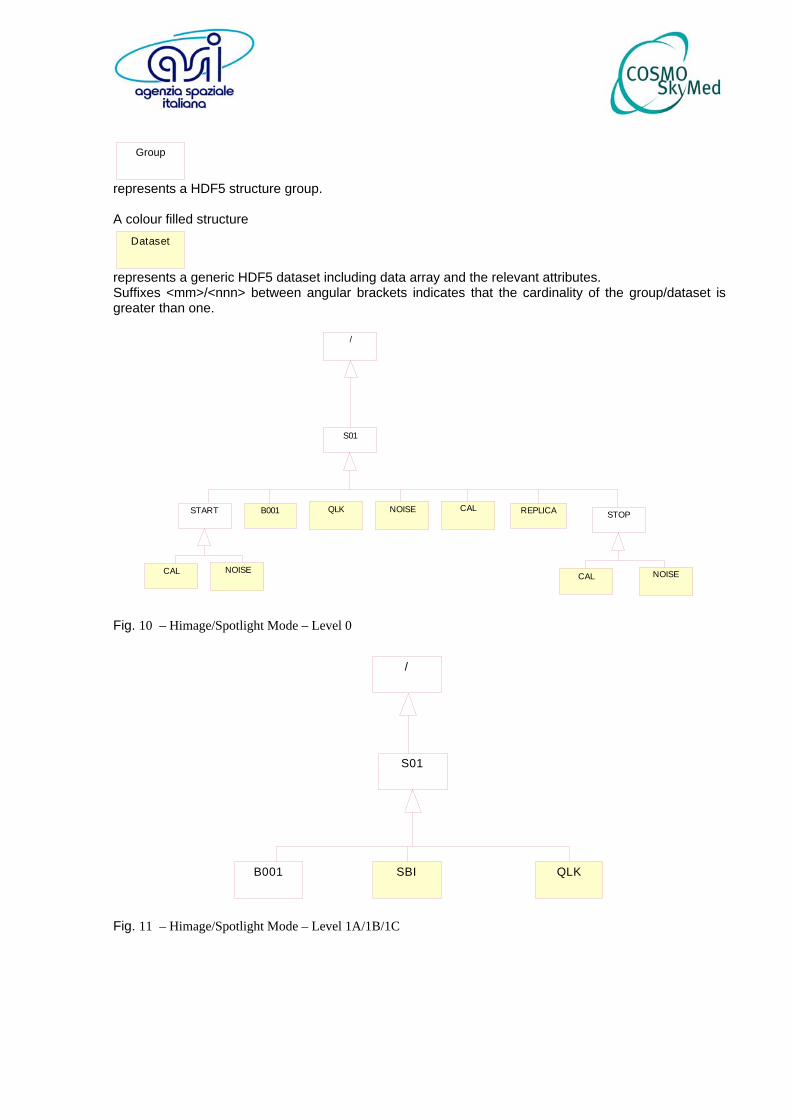
Group
represents a HDF5 structure group. A colour filled structure
Dataset
represents a generic HDF5 dataset including data array and the relevant attributes. Suffixes <mm>/<nnn> between angular brackets indicates that the cardinality of the group/dataset is greater than one.
/
S01
B001 QLK CAL
CAL
NOISE STOPSTART
CAL NOISE NOISE
REPLICA
Fig. 10 – Himage/Spotlight Mode – Level 0
SBI
/
QLKB001
S01
Fig. 11 – Himage/Spotlight Mode – Level 1A/1B/1C
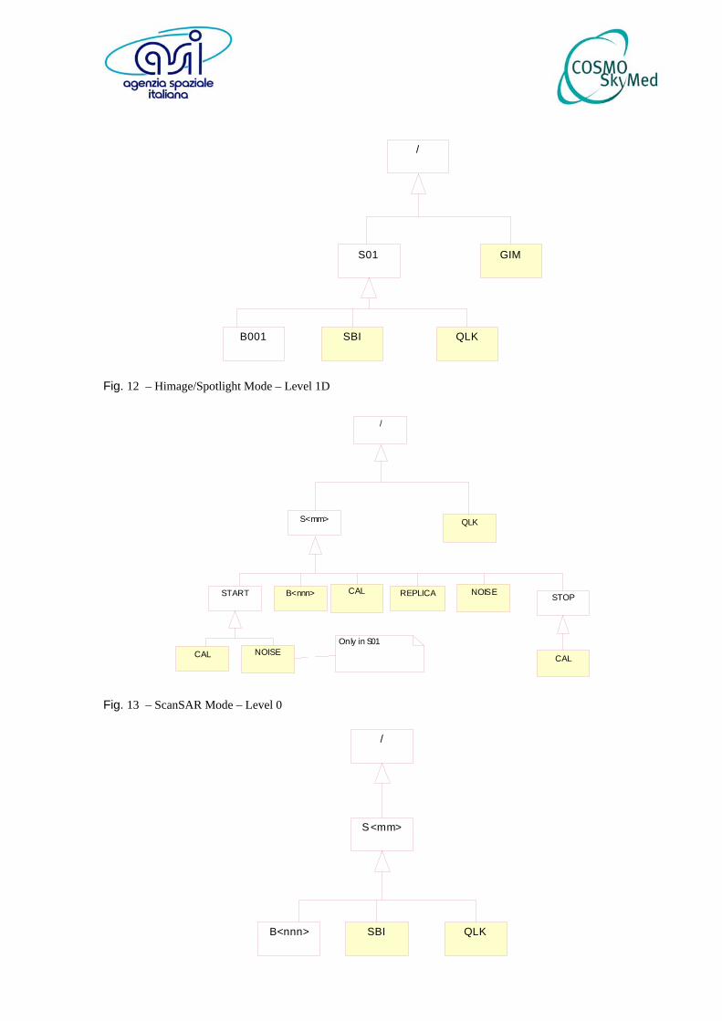
/
SBI QLK
GIM
B001
S01
Fig. 12 – Himage/Spotlight Mode – Level 1D
/
S<mm>
B<nnn>
QLK
CAL
Only in S01
CAL
NOISE STOPSTART
CAL NOISE
REPLICA
Fig. 13 – ScanSAR Mode – Level 0
/
S<mm>
B<nnn> QLKSBI
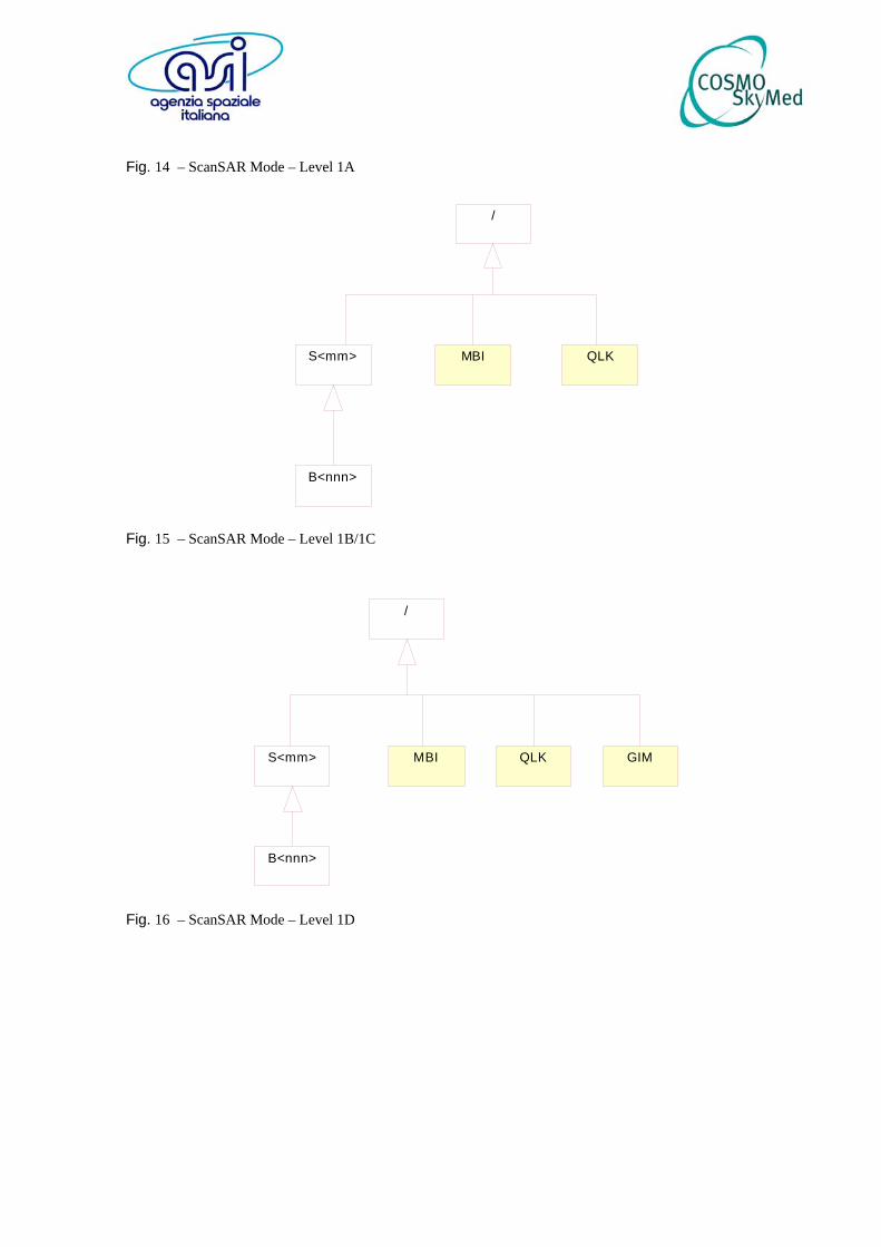
Fig. 14 – ScanSAR Mode – Level 1A
/
S<mm>
B<nnn>
QLKMBI
Fig. 15 – ScanSAR Mode – Level 1B/1C
/
S<mm> MBI
B<nnn>
QLK GIM
Fig. 16 – ScanSAR Mode – Level 1D
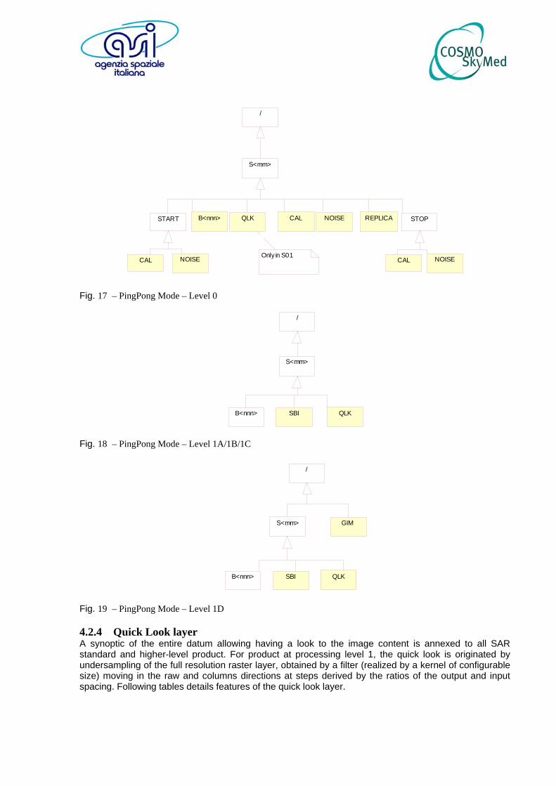
/
S<mm>
B<nnn> QLK NOISECALSTART STOP
CAL NOISE CAL NOISE
REPLICA
Only in S01
Fig. 17 – PingPong Mode – Level 0
/
S<mm>
B<nnn> SBI QLK
Fig. 18 – PingPong Mode – Level 1A/1B/1C
GIM
/
S<mm>
B<nnn> SBI QLK
Fig. 19 – PingPong Mode – Level 1D
4.2.4 Quick Look layer A synoptic of the entire datum allowing having a look to the image content is annexed to all SAR standard and higher-level product. For product at processing level 1, the quick look is originated by undersampling of the full resolution raster layer, obtained by a filter (realized by a kernel of configurable size) moving in the raw and columns directions at steps derived by the ratios of the output and input spacing. Following tables details features of the quick look layer.
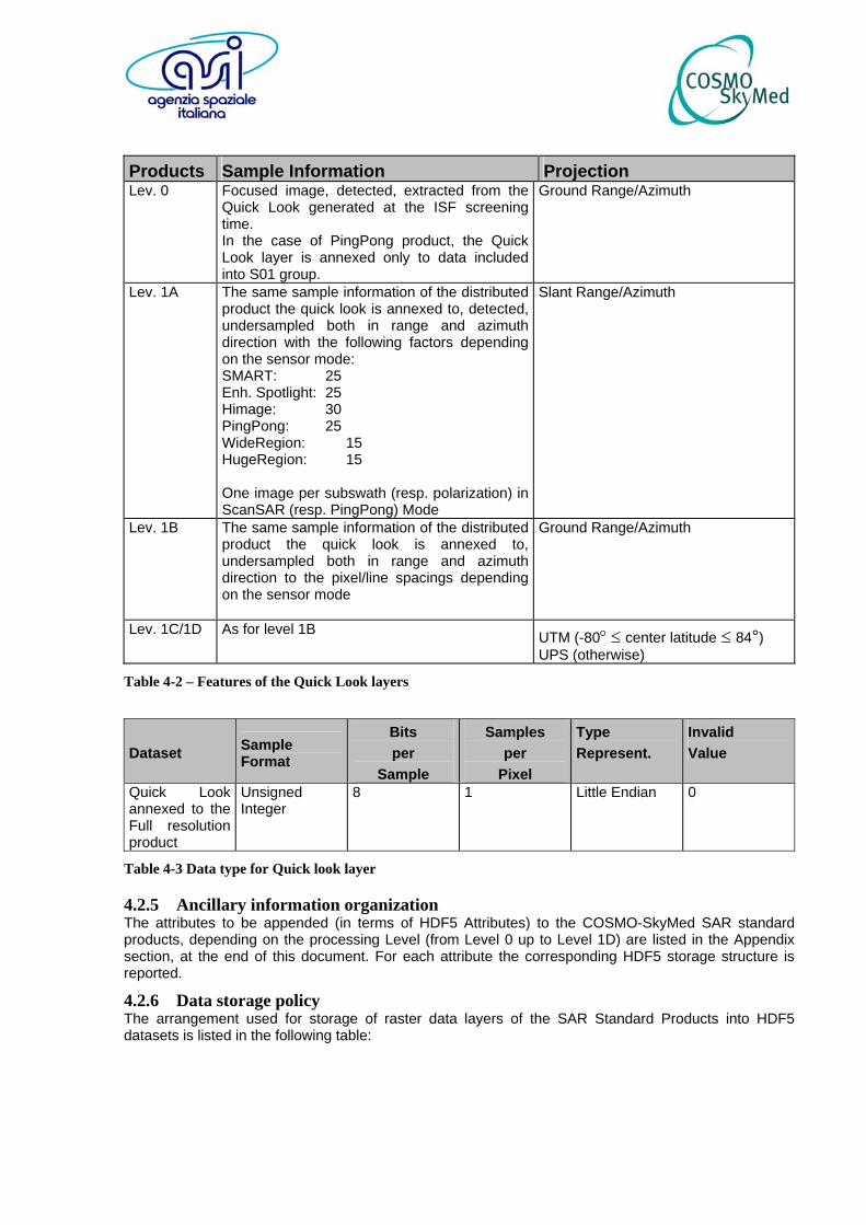
Products Sample Information Projection Lev. 0 Focused image, detected, extracted from the
Quick Look generated at the ISF screening time. In the case of PingPong product, the Quick Look layer is annexed only to data included into S01 group.
Ground Range/Azimuth
Lev. 1A The same sample information of the distributed product the quick look is annexed to, detected, undersampled both in range and azimuth direction with the following factors depending on the sensor mode: SMART: 25 Enh. Spotlight: 25 Himage: 30 PingPong: 25 WideRegion: 15 HugeRegion: 15 One image per subswath (resp. polarization) in ScanSAR (resp. PingPong) Mode
Slant Range/Azimuth
Lev. 1B The same sample information of the distributed product the quick look is annexed to, undersampled both in range and azimuth direction to the pixel/line spacings depending on the sensor mode
Ground Range/Azimuth
Lev. 1C/1D As for level 1B UTM (-80° ≤ center latitude ≤ 84°) UPS (otherwise)
Table 4-2 – Features of the Quick Look layers
Dataset Sample Format
Bits per
Sample
Samples per
Pixel
Type Represent.
Invalid Value
Quick Look annexed to the Full resolution product
Unsigned Integer
8 1 Little Endian 0
Table 4-3 Data type for Quick look layer
4.2.5 Ancillary information organization The attributes to be appended (in terms of HDF5 Attributes) to the COSMO-SkyMed SAR standard products, depending on the processing Level (from Level 0 up to Level 1D) are listed in the Appendix section, at the end of this document. For each attribute the corresponding HDF5 storage structure is reported.
4.2.6 Data storage policy The arrangement used for storage of raster data layers of the SAR Standard Products into HDF5 datasets is listed in the following table:

Samples per pixel HDF5 data type Two (Complex data)
Tri-dimensional array having: • the first dimension (the slowest varying) corresponding to the
number of lines of the data array • the second dimension corresponding to the number of columns of
the data array • the third dimension (the most fast varying) corresponding to the pixel
depth, hence used for representation of Real and Imaginary part of each pixel
• Such representation, will be used for complex types independently on the sample format (byte, short, integer, long, long long, float, double) and sign (signed, unsigned).
Data organization in file is shoed in the following schema
Line 2 Line 1
I1 Q1 ... ... ... ... In Qn I1 Q1 ... ... ... ... In Qn ... ... One (Real data)
Bi-dimensional array having: • the first dimension (the slowest varying) corresponding to the
number of lines of the data array • the second dimension corresponding to the number of columns of
the data array Such representation will be used for images on single-sample pixel, independently on the sample format (byte, short, integer, long, long long, float, double) and sign (signed, unsigned)
Line 2 Line 1
P1 P2 ... ... ... ... ... Pn P1 P2 ... ... ... ... ... Pn ... ... The following chunking policy for data storage is recommended. Dimension Chunk Size Image Length (Lines) 128 Image Width (Columns) 128 Image Depth (Samples) 2
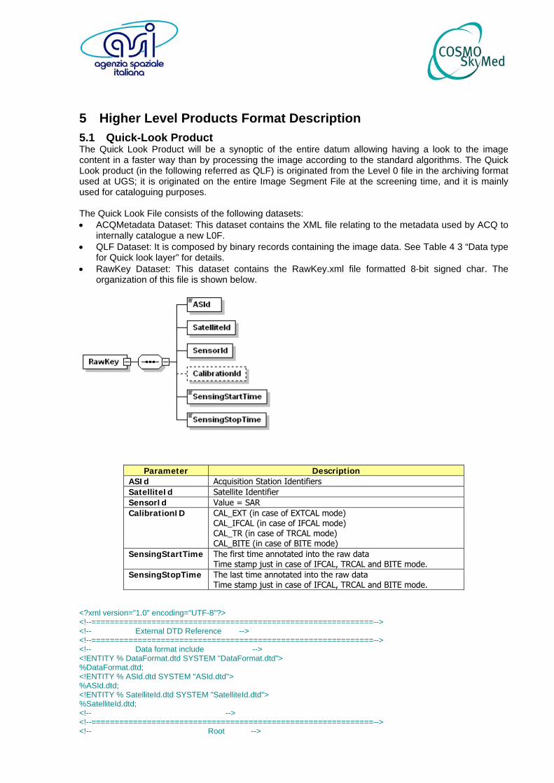
5 Higher Level Products Format Description 5.1 Quick-Look Product The Quick Look Product will be a synoptic of the entire datum allowing having a look to the image content in a faster way than by processing the image according to the standard algorithms. The Quick Look product (in the following referred as QLF) is originated from the Level 0 file in the archiving format used at UGS; it is originated on the entire Image Segment File at the screening time, and it is mainly used for cataloguing purposes. The Quick Look File consists of the following datasets: • ACQMetadata Dataset: This dataset contains the XML file relating to the metadata used by ACQ to
internally catalogue a new L0F. • QLF Dataset: It is composed by binary records containing the image data. See Table 4 3 “Data type
for Quick look layer” for details. • RawKey Dataset: This dataset contains the RawKey.xml file formatted 8-bit signed char. The
organization of this file is shown below.
Parameter Description ASId Acquisition Station Identifiers SatelliteId Satellite Identifier SensorId Value = SAR CalibrationID CAL_EXT (in case of EXTCAL mode)
CAL_IFCAL (in case of IFCAL mode) CAL_TR (in case of TRCAL mode) CAL_BITE (in case of BITE mode)
SensingStartTime The first time annotated into the raw data Time stamp just in case of IFCAL, TRCAL and BITE mode.
SensingStopTime The last time annotated into the raw data Time stamp just in case of IFCAL, TRCAL and BITE mode.
<?xml version="1.0" encoding="UTF-8"?> <!--=============================================================--> <!-- External DTD Reference --> <!--=============================================================--> <!-- Data format include --> <!ENTITY % DataFormat.dtd SYSTEM "DataFormat.dtd"> %DataFormat.dtd; <!ENTITY % ASId.dtd SYSTEM "ASId.dtd"> %ASId.dtd; <!ENTITY % SatelliteId.dtd SYSTEM "SatelliteId.dtd"> %SatelliteId.dtd; <!-- --> <!--=============================================================--> <!-- Root -->
<!--=============================================================--> <!ELEMENT RawKey (ASId, SatelliteId, SensorId, CalibrationId?, SensingStartTime, SensingStopTime)> <!--=============================================================--> <!-- List of elements --> <!--=============================================================--> <!ELEMENT SensorId EMPTY> <!ATTLIST SensorId Value (SAR) #REQUIRED %StringFormat; > <!ELEMENT CalibrationId EMPTY> <!ATTLIST CalibrationId Value (CAL_EXT | CAL_TR | CAL_IF | BITE) #REQUIRED %StringFormat; > <!ELEMENT SensingStartTime (#PCDATA)> <!ATTLIST SensingStartTime %DateFormat; Format CDATA #FIXED "YYYY-MM-DD hh:mm:ss.nnnnnn" > <!ELEMENT SensingStopTime (#PCDATA)> <!ATTLIST SensingStopTime %DateFormat; Format CDATA #FIXED "YYYY-MM-DD hh:mm:ss.nnnnnn" > <!-- end RawKey.dtd --> ~ ~ Image specification of the QLF product, are listed in section #4.2.4.
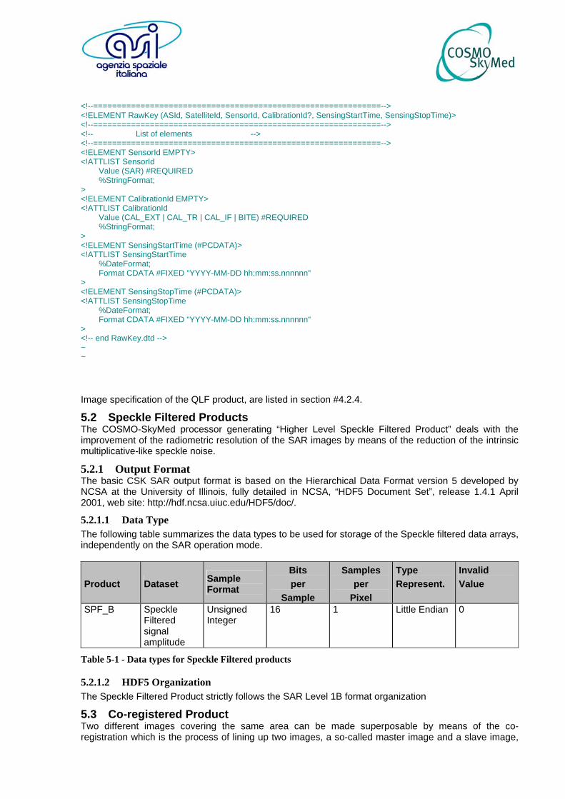
5.2 Speckle Filtered Products The COSMO-SkyMed processor generating “Higher Level Speckle Filtered Product” deals with the improvement of the radiometric resolution of the SAR images by means of the reduction of the intrinsic multiplicative-like speckle noise.
5.2.1 Output Format The basic CSK SAR output format is based on the Hierarchical Data Format version 5 developed by NCSA at the University of Illinois, fully detailed in NCSA, “HDF5 Document Set”, release 1.4.1 April 2001, web site: http://hdf.ncsa.uiuc.edu/HDF5/doc/.
5.2.1.1 Data Type The following table summarizes the data types to be used for storage of the Speckle filtered data arrays, independently on the SAR operation mode.
Product Dataset Sample Format
Bits per
Sample
Samples per
Pixel
Type Represent.
Invalid Value
SPF_B Speckle Filtered signal amplitude
Unsigned Integer
16 1 Little Endian 0
Table 5-1 - Data types for Speckle Filtered products
5.2.1.2 HDF5 Organization The Speckle Filtered Product strictly follows the SAR Level 1B format organization
5.3 Co-registered Product Two different images covering the same area can be made superposable by means of the co-registration which is the process of lining up two images, a so-called master image and a slave image,
in a way that they fit exactly on top of each other without adding artifacts in the image intensity and phase components.
5.3.1 Output Format The basic CSK SAR output format is based on the Hierarchical Data Format version 5 developed by NCSA at the University of Illinois, fully detailed in NCSA, “HDF5 Document Set”, release 1.4.1 April 2001, web site: http://hdf.ncsa.uiuc.edu/HDF5/doc/.
5.3.1.1 Data Type The following table summarizes the data types to be used for storage of the co-registered data arrays, depending on the processing Level (Level 1A or Level 1B) of the input data to the coregistration processor, independently on the SAR operation mode.
Product Dataset Sample Format Bits per
Sample
Samples per
Pixel
Type Represent.
Invalid Value
CRG_A Coregistered SAR Data
Signed Integer 16 2 Little Endian [0, 0]
CRG_B Coregistered SAR Data
Unsigned Integer 16 1 Little Endian 0
Table 5-2 Data types for Co-registered products
5.3.1.2 HDF5 Organization The Co-registered Product strictly follows the SAR Level 1A and 1B format organization, depending on the processing level of the input images.
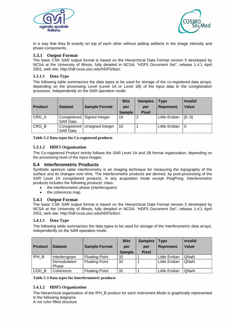
5.4 Interferometric Products Synthetic aperture radar interferometry is an imaging technique for measuring the topography of the surface and its changes over time. The Interferometric products are derived, by post-processing of the SAR Level 1A coregistered products, in any acquisition mode except PingPong. Interferometric products includes the following products’ class:
• the interferometric phase (interferogram) • the coherence map.
5.4.1 Output Format The basic CSK SAR output format is based on the Hierarchical Data Format version 5 developed by NCSA at the University of Illinois, fully detailed in NCSA, “HDF5 Document Set”, release 1.4.1 April 2001, web site: http://hdf.ncsa.uiuc.edu/HDF5/doc/.
5.4.1.1 Data Type The following table summarizes the data types to be used for storage of the Interferometric data arrays, independently on the SAR operation mode.
Product Dataset Sample Format Bits per
Sample
Samples per
Pixel
Type Represent.
Invalid Value
Interferogram Floating Point 32 1 Little Endian QNaN IPH_B Demodulation Phase
Floating Point 32 1 Little Endian QNaN
COH_B Coherence Floating Point 32 1 Little Endian QNaN
Table 5-3 Data types for Interferometric products
5.4.1.2 HDF5 Organization The hierarchical organization of the IPH_B product for each Instrument Mode is graphically represented in the following diagrams. A not color filled structure
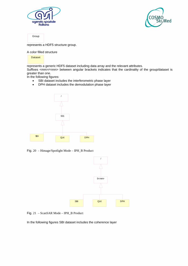
Group
represents a HDF5 structure group. A color filled structure
Dataset
represents a generic HDF5 dataset including data array and the relevant attributes. Suffixes <mm>/<nnn> between angular brackets indicates that the cardinality of the group/dataset is greater than one. In the following figures:
• SBI dataset includes the interferometric phase layer • DPH dataset includes the demodulation phase layer
/
QLK
S01
SBI DPH
Fig. 20 – Himage/Spotlight Mode – IPH_B Product
/
S<mm>
QLKSBI DPH
Fig. 21 – ScanSAR Mode – IPH_B Product
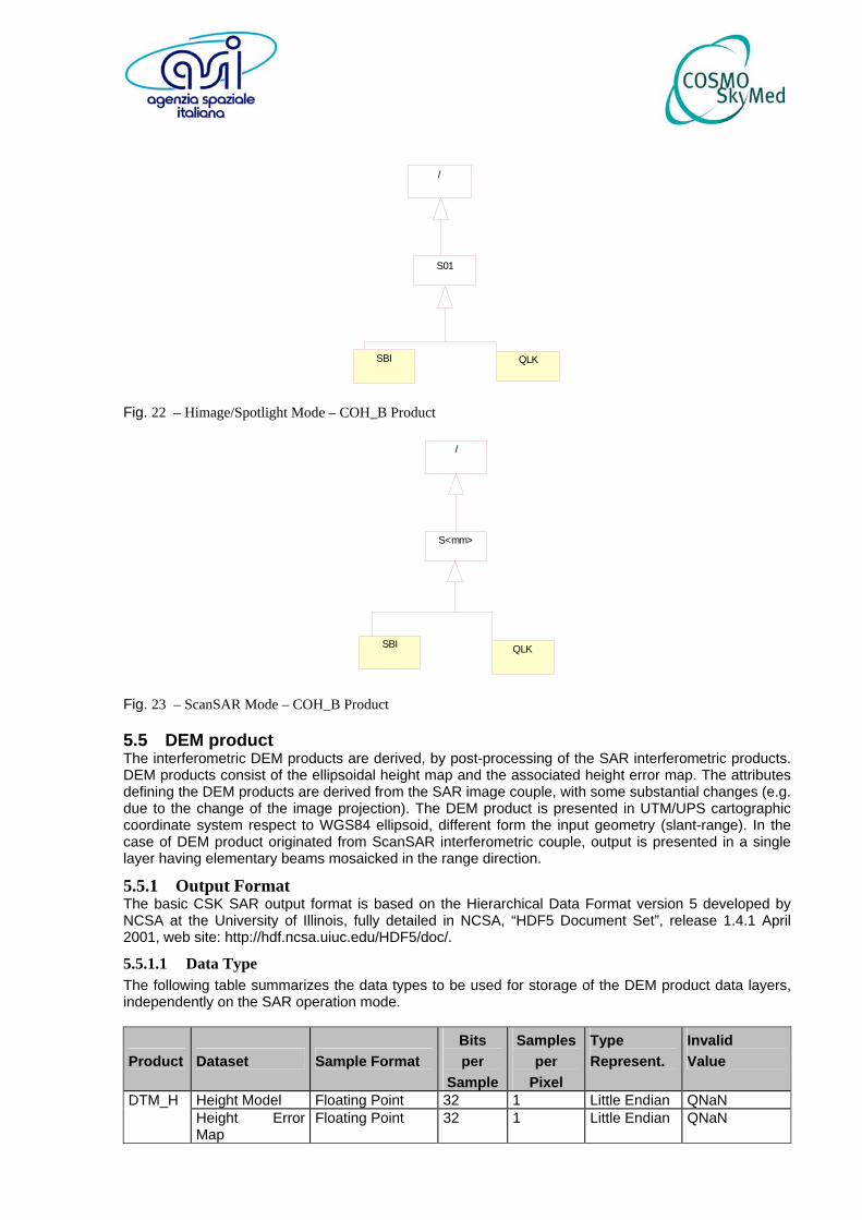
In the following figures SBI dataset includes the coherence layer
/
QLK
S01
SBI
Fig. 22 – Himage/Spotlight Mode – COH_B Product
/
S<mm>
QLKSBI
Fig. 23 – ScanSAR Mode – COH_B Product
5.5 DEM product The interferometric DEM products are derived, by post-processing of the SAR interferometric products. DEM products consist of the ellipsoidal height map and the associated height error map. The attributes defining the DEM products are derived from the SAR image couple, with some substantial changes (e.g. due to the change of the image projection). The DEM product is presented in UTM/UPS cartographic coordinate system respect to WGS84 ellipsoid, different form the input geometry (slant-range). In the case of DEM product originated from ScanSAR interferometric couple, output is presented in a single layer having elementary beams mosaicked in the range direction.
5.5.1 Output Format The basic CSK SAR output format is based on the Hierarchical Data Format version 5 developed by NCSA at the University of Illinois, fully detailed in NCSA, “HDF5 Document Set”, release 1.4.1 April 2001, web site: http://hdf.ncsa.uiuc.edu/HDF5/doc/.
5.5.1.1 Data Type The following table summarizes the data types to be used for storage of the DEM product data layers, independently on the SAR operation mode.
Product Dataset Sample Format Bits per
Sample
Samples per
Pixel
Type Represent.
Invalid Value
Height Model Floating Point 32 1 Little Endian QNaN DTM_H Height Error Map
Floating Point 32 1 Little Endian QNaN
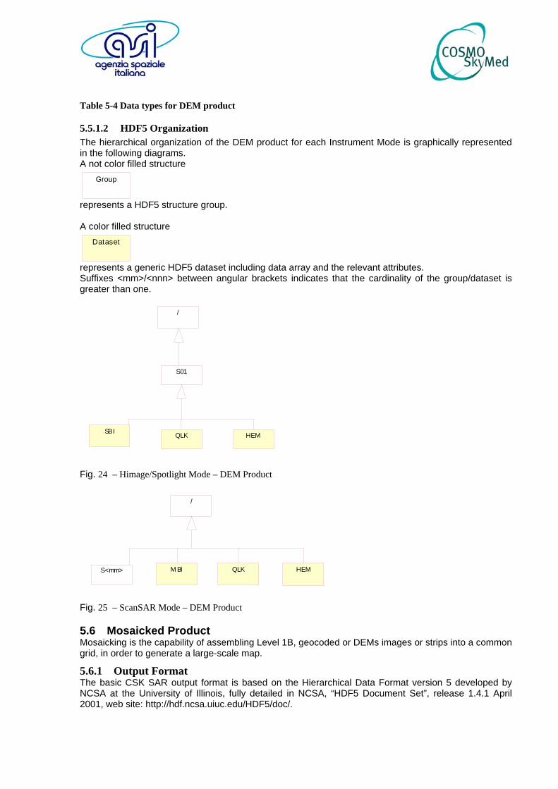
Table 5-4 Data types for DEM product
5.5.1.2 HDF5 Organization The hierarchical organization of the DEM product for each Instrument Mode is graphically represented in the following diagrams. A not color filled structure
Group
represents a HDF5 structure group. A color filled structure
Dataset
represents a generic HDF5 dataset including data array and the relevant attributes. Suffixes <mm>/<nnn> between angular brackets indicates that the cardinality of the group/dataset is greater than one.
/
QLK
S01
SBI HEM
Fig. 24 – Himage/Spotlight Mode – DEM Product
/
S<mm> QLKM BI HEM
Fig. 25 – ScanSAR Mode – DEM Product
5.6 Mosaicked Product Mosaicking is the capability of assembling Level 1B, geocoded or DEMs images or strips into a common grid, in order to generate a large-scale map.
5.6.1 Output Format The basic CSK SAR output format is based on the Hierarchical Data Format version 5 developed by NCSA at the University of Illinois, fully detailed in NCSA, “HDF5 Document Set”, release 1.4.1 April 2001, web site: http://hdf.ncsa.uiuc.edu/HDF5/doc/.
5.6.1.1 Data Type The following table summarizes the data types to be used for storage of the Mosaicked data arrays, independently on the SAR operation mode.
Product Dataset Sample Format Bits per
Sample
Samples per
Pixel
Type Represent.
Invalid Value
MOS_B SAR Image Unsigned Integer 16 1 Little Endian 0 MOS_C SAR Image Unsigned Integer 16 1 Little Endian 0 MOS_D SAR Image Unsigned Integer 16 1 Little Endian 0
Heght Float 32 1 Little Endian QNaN MOS_H Height Error Map
Float 32 1 Little Endian QNaN
Table 5-5 - Data types for Mosaicked products
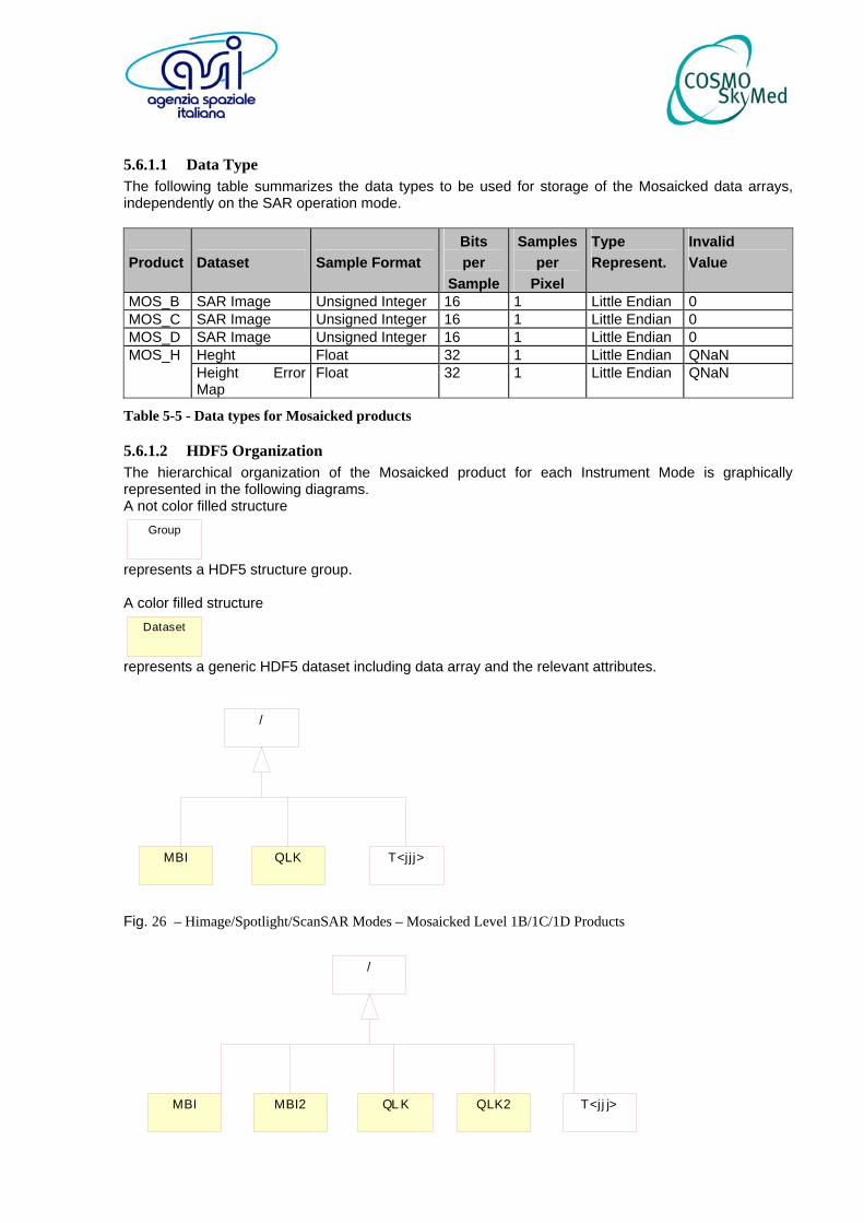
5.6.1.2 HDF5 Organization The hierarchical organization of the Mosaicked product for each Instrument Mode is graphically represented in the following diagrams. A not color filled structure
Group
represents a HDF5 structure group. A color filled structure
Dataset
represents a generic HDF5 dataset including data array and the relevant attributes.
/
QLKMBI T<jjj>
Fig. 26 – Himage/Spotlight/ScanSAR Modes – Mosaicked Level 1B/1C/1D Products
MBI2
/
QL KMBI T<jj j>QLK2
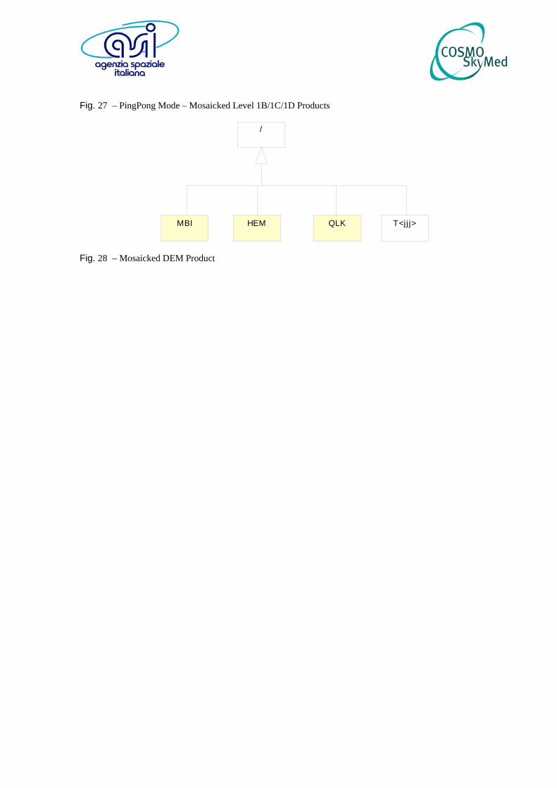
Fig. 27 – PingPong Mode – Mosaicked Level 1B/1C/1D Products
/
QLKMBI HEM T<jj j>
Fig. 28 – Mosaicked DEM Product
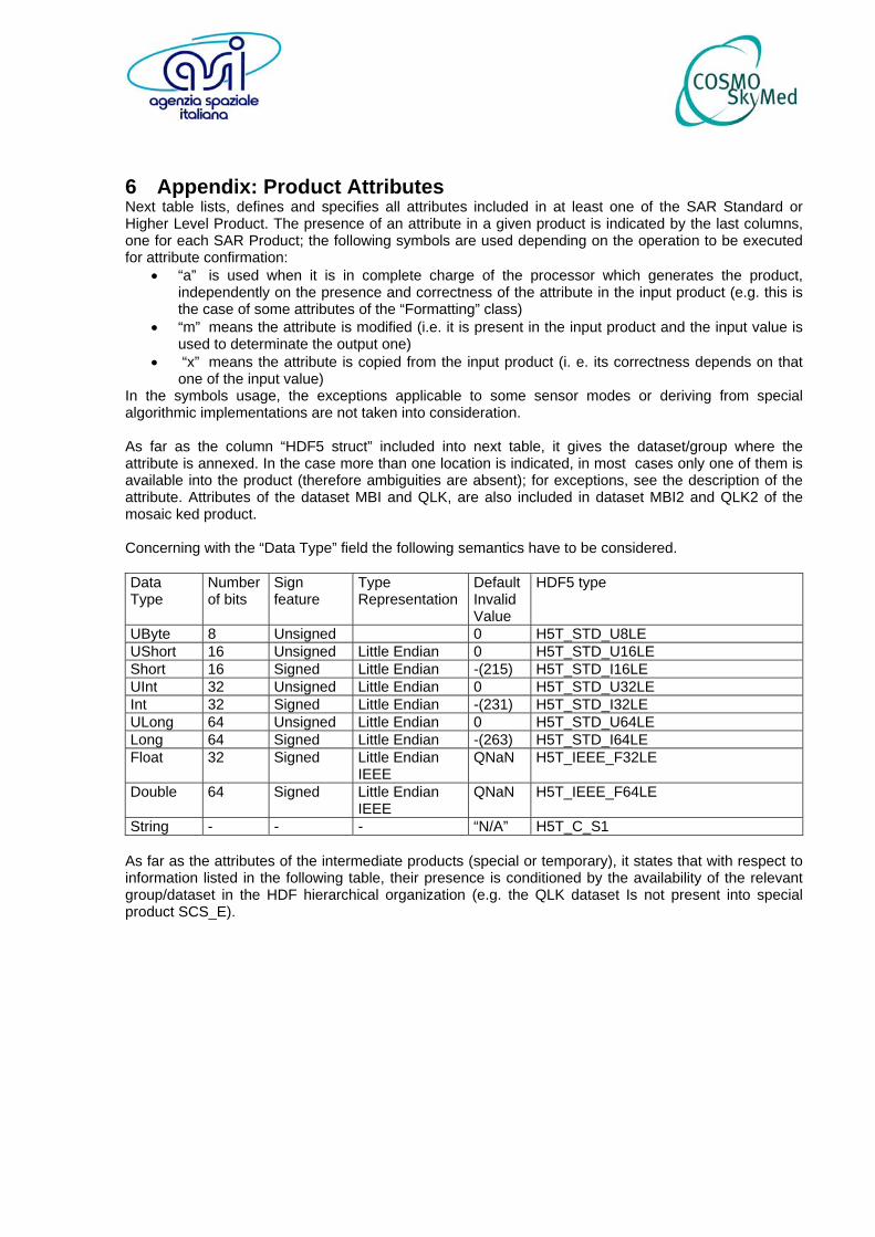
6 Appendix: Product Attributes Next table lists, defines and specifies all attributes included in at least one of the SAR Standard or Higher Level Product. The presence of an attribute in a given product is indicated by the last columns, one for each SAR Product; the following symbols are used depending on the operation to be executed for attribute confirmation:
• “a” is used when it is in complete charge of the processor which generates the product, independently on the presence and correctness of the attribute in the input product (e.g. this is the case of some attributes of the “Formatting” class)
• “m” means the attribute is modified (i.e. it is present in the input product and the input value is used to determinate the output one)
• “x” means the attribute is copied from the input product (i. e. its correctness depends on that one of the input value)
In the symbols usage, the exceptions applicable to some sensor modes or deriving from special algorithmic implementations are not taken into consideration. As far as the column “HDF5 struct” included into next table, it gives the dataset/group where the attribute is annexed. In the case more than one location is indicated, in most cases only one of them is available into the product (therefore ambiguities are absent); for exceptions, see the description of the attribute. Attributes of the dataset MBI and QLK, are also included in dataset MBI2 and QLK2 of the mosaic ked product. Concerning with the “Data Type” field the following semantics have to be considered. Data Type
Number of bits
Sign feature
Type Representation
Default Invalid Value
HDF5 type
UByte 8 Unsigned 0 H5T_STD_U8LE UShort 16 Unsigned Little Endian 0 H5T_STD_U16LE Short 16 Signed Little Endian -(215) H5T_STD_I16LE UInt 32 Unsigned Little Endian 0 H5T_STD_U32LE Int 32 Signed Little Endian -(231) H5T_STD_I32LE ULong 64 Unsigned Little Endian 0 H5T_STD_U64LE Long 64 Signed Little Endian -(263) H5T_STD_I64LE Float 32 Signed Little Endian
IEEE QNaN H5T_IEEE_F32LE
Double 64 Signed Little Endian IEEE
QNaN H5T_IEEE_F64LE
String - - - “N/A” H5T_C_S1 As far as the attributes of the intermediate products (special or temporary), it states that with respect to information listed in the following table, their presence is conditioned by the availability of the relevant group/dataset in the HDF hierarchical organization (e.g. the QLK dataset Is not present into special product SCS_E).
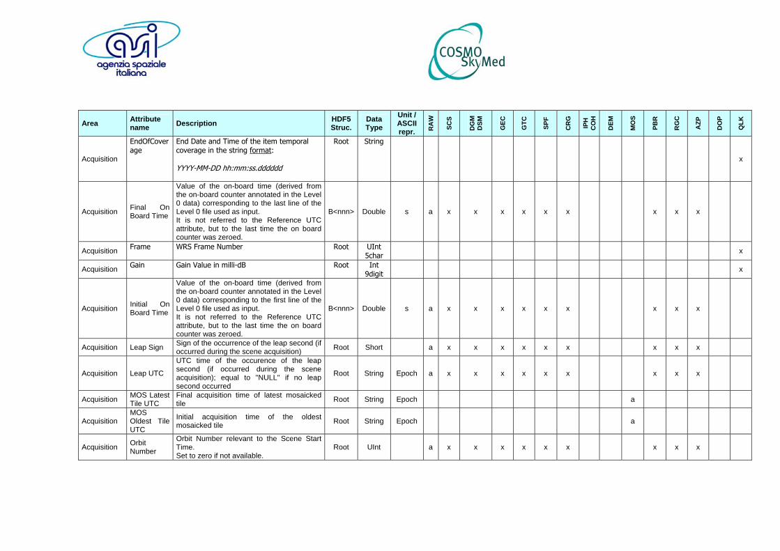
Area Attribute name Description HDF5
Struc. Data Type
Unit /ASCII repr. R
AW
SCS
DG
M
DSM
GEC
GTC
SPF
CR
G
IPH
C
OH
DEM
MO
S
PBR
RG
C
AZP
DO
P
QLK
Acquisition
EndOfCoverage
End Date and Time of the item temporal coverage in the string format: YYYY-MM-DD hh:mm:ss.dddddd
Root String
x
Acquisition Final On Board Time
Value of the on-board time (derived from the on-board counter annotated in the Level 0 data) corresponding to the last line of the Level 0 file used as input. It is not referred to the Reference UTC attribute, but to the last time the on board counter was zeroed.
B<nnn> Double s a x x x x x x x x x
Acquisition Frame WRS Frame Number Root UInt 5char
x
Acquisition Gain Gain Value in milli-dB Root Int 9digit
x
Acquisition Initial On Board Time
Value of the on-board time (derived from the on-board counter annotated in the Level 0 data) corresponding to the first line of the Level 0 file used as input. It is not referred to the Reference UTC attribute, but to the last time the on board counter was zeroed.
B<nnn> Double s a x x x x x x x x x
Acquisition Leap Sign Sign of the occurrence of the leap second (if occurred during the scene acquisition) Root Short a x x x x x x x x x
Acquisition Leap UTC
UTC time of the occurence of the leap second (if occurred during the scene acquisition); equal to "NULL" if no leap second occurred
Root String Epoch a x x x x x x x x x
Acquisition MOS Latest Tile UTC
Final acquisition time of latest mosaicked tile Root String Epoch a
Acquisition MOS Oldest Tile UTC
Initial acquisition time of the oldest mosaicked tile Root String Epoch a
Acquisition Orbit Number
Orbit Number relevant to the Scene Start Time. Set to zero if not available.
Root UInt a x x x x x x x x x

Area Attribute name Description HDF5
Struc. Data Type
Unit /ASCII repr. R
AW
SCS
DG
M
DSM
GEC
GTC
SPF
CR
G
IPH
C
OH
DEM
MO
S
PBR
RG
C
AZP
DO
P
QLK
Acquisition
OrbitNumber
Absolute Orbit Number corresponds to ISF start time where the ISF start time is intended the same of the field StartOfCoverage.
Root UInt 8char
x
Acquisition
PassEquatorXLongitude
Nadir Equator Crossing Longitude for this Pass Example: 160.98
Root Double Int
digits: 3 decimal
s: 2
x
Acquisition
Polarization Polarization. Allowed values: VV Vertical Vertical HH Horizontal Horizontal VH Vertical Horizontal HV Horizontal Vertical CO Co-Polar CH Cross-Polar H CV Cross-Polar V
Root String 2char
x
Acquisition Programmed Image ID
Image ID as it was programmed by Ground Segment and downlinked in the packet header
Root UShort a x x x x x x x x x

Area Attribute name Description HDF5
Struc. Data Type
Unit /ASCII repr. R
AW
SCS
DG
M
DSM
GEC
GTC
SPF
CR
G
IPH
C
OH
DEM
MO
S
PBR
RG
C
AZP
DO
P
QLK
Acquisition
QuickLookFirstLineTime
Date and Time at Zero doppler of the first line of the QLF layer in the string format: YYYY-MM-DD hh:mm:ss.dddddd the possible reverse Late/Early is taken into account
Root String
x
Acquisition
QuickLookLastLineTime
Date and Time at Zero doppler of the last line of the QLF layer in the string format: YYYY-MM-DD hh:mm:ss.dddddd the possible reverse Late/Early is taken into account
Root String
x
Acquisition Scene Sensing Start UTC
Initial acquisition time of the scene in UTC, derived from the OBT extracted from the downlinked product. Attribute updating is applicable in the case of processing of image portion starting from Level 0 data. For mosaicked products it is annexed only to tiles. Set to invalid value in the case of mosaicked DEM
Root T<jjj> String Epoch a m m x x x x x x m m
Acquisition Scene Sensing Stop UTC
Final acquisition time of the scene in UTC, derived from the OBT extracted from the downlinked product. Attribute updating is applicable in the case of processing of image portion starting from Level 0 data. For mosaicked products it is annexed only to tiles. Set to invalid value in the case of mosaicked DEM
Root T<jjj> String Epoch a m m x x x x x x m m
Acquisition Selective Availability Status
Status of the Selective Availability during the acquisition, affecting Orbital Data derived by GPS Instrument
Root String a x x x x x x x x x

Area Attribute name Description HDF5
Struc. Data Type
Unit /ASCII repr. R
AW
SCS
DG
M
DSM
GEC
GTC
SPF
CR
G
IPH
C
OH
DEM
MO
S
PBR
RG
C
AZP
DO
P
QLK
Acquisition
SensorModeDescription
Descriptive text of specific sensor mode Allowed values: SP_ENHANCED SP_SMART SCN_WIDE SCN_HUGE STR_HIMAGE STR_PINGPONG
Root String 50char
x
Acquisition
SensorModeId
Specific sensor mode Allowed values: S2 S1 WR HR HI PP
Root String 20char
x
Acquisition
StartOfCoverage
Start Date and Time of the item temporal coverage in the string format: YYYY-MM-DD hh:mm:ss.dddddd
Root String
x
Acquisition Track WRS Track Number Root UInt 5char
x
Calibration ADC Characterization
Look Up Table for ADC Characterization; it associates the signal power detected in the 8 bits RAW data to the ideal analog level in dB. For future usage
Root Double(256, 2) a x x x x x x x x x
Calibration ADC Compensation
Flag showing the application of the ADC compensation. For future usage
Root UByte a x x x x x x
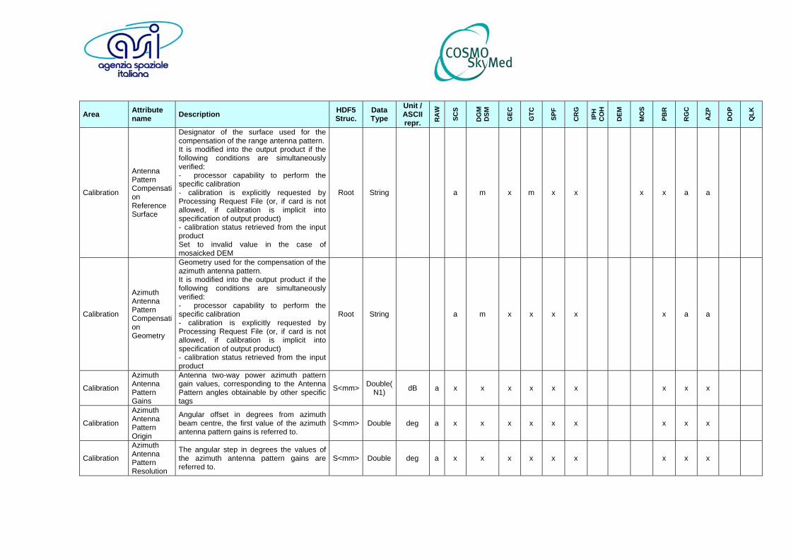
Area Attribute name Description HDF5
Struc. Data Type
Unit /ASCII repr. R
AW
SCS
DG
M
DSM
GEC
GTC
SPF
CR
G
IPH
C
OH
DEM
MO
S
PBR
RG
C
AZP
DO
P
QLK
Calibration
Antenna Pattern Compensation Reference Surface
Designator of the surface used for the compensation of the range antenna pattern.It is modified into the output product if the following conditions are simultaneously verified: - processor capability to perform the specific calibration - calibration is explicitly requested by Processing Request File (or, if card is not allowed, if calibration is implicit into specification of output product) - calibration status retrieved from the input product Set to invalid value in the case of mosaicked DEM
Root String a m x m x x x x a a
Calibration
Azimuth Antenna Pattern Compensation Geometry
Geometry used for the compensation of the azimuth antenna pattern. It is modified into the output product if the following conditions are simultaneously verified: - processor capability to perform the specific calibration - calibration is explicitly requested by Processing Request File (or, if card is not allowed, if calibration is implicit into specification of output product) - calibration status retrieved from the input product
Root String a m x x x x x a a
Calibration
Azimuth Antenna Pattern Gains
Antenna two-way power azimuth pattern gain values, corresponding to the Antenna Pattern angles obtainable by other specific tags
S<mm> Double(N1) dB a x x x x x x x x x
Calibration
Azimuth Antenna Pattern Origin
Angular offset in degrees from azimuth beam centre, the first value of the azimuth antenna pattern gains is referred to.
S<mm> Double deg a x x x x x x x x x
Calibration
Azimuth Antenna Pattern Resolution
The angular step in degrees the values of the azimuth antenna pattern gains are referred to.
S<mm> Double deg a x x x x x x x x x

Area Attribute name Description HDF5
Struc. Data Type
Unit /ASCII repr. R
AW
SCS
DG
M
DSM
GEC
GTC
SPF
CR
G
IPH
C
OH
DEM
MO
S
PBR
RG
C
AZP
DO
P
QLK
Calibration Calibration Constant
It is the Calibration Constant value (K) of the subswath. It includes all constant proportionality terms between the target energy in the input product and the actual backscattering of the scene. It excludes terms related to Range Spreading Loss, Incidence angle and Antenna Pattern compensation operators. The multiplier term (1/sqrt(K)) have to be applied to calibrate the signal amplitude. It is applied to the output SAR image if the following conditions are simultaneously verified: - processor capability to perform the specific calibration - calibration is explicitly requested by Processing Request File (or, if card is not allowed, if calibration is implicit into specification of output product) - calibration status retrieved from the input product is set to "Not Calibrated". The attribute, in any case, must be left unchanged.
S<mm> Double a x x x x x x x x x
Calibration
Calibration Constant Compensation Flag
Flag showing the application of the calibration constant. It is modified into the output product if the following conditions are simultaneously verified: - processor capability to perform the specific calibration - calibration is explicitly requested by Processing Request File (or, if card is not allowed, if calibration is implicit into specification of output product) - calibration status retrieved from the input product Set to invalid value in the case of mosaicked DEM
Root UByte a m x m x x m x a a

Area Attribute name Description HDF5
Struc. Data Type
Unit /ASCII repr. R
AW
SCS
DG
M
DSM
GEC
GTC
SPF
CR
G
IPH
C
OH
DEM
MO
S
PBR
RG
C
AZP
DO
P
QLK
Calibration
Calibration Constant Estimation UTC
Calibration constant estimation date S<mm> String Epoch a x x x m x x x x x
Calibration
Incidence Angle Compensation Geometry
Geometry used for the compensation of the incidence angle. It is modified into the output product if the following conditions are simultaneously verified: - processor capability to perform the specific calibration - calibration is explicitly requested by Processing Request File (or, if card is not allowed, if calibration is implicit into specification of output product) - calibration status retrieved from the input product
Root String a m x m x x x a a
Calibration
Incidence Angle Compensation Reference Surface
Designator of the surface used for the compensation of the incidence angle. It is modified into the output product if the following conditions are simultaneously verified: - processor capability to perform the specific calibration - calibration is explicitly requested by Processing Request File (or, if card is not allowed, if calibration is implicit into specification of output product) - calibration status retrieved from the input product Set to invalid value in the case of mosaicked DEM
Root String a m x m x x x x a a
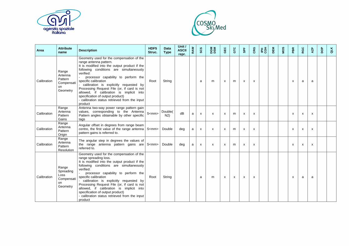
Area Attribute name Description HDF5
Struc. Data Type
Unit /ASCII repr. R
AW
SCS
DG
M
DSM
GEC
GTC
SPF
CR
G
IPH
C
OH
DEM
MO
S
PBR
RG
C
AZP
DO
P
QLK
Calibration
Range Antenna Pattern Compensation Geometry
Geometry used for the compensation of the range antenna pattern. It is modified into the output product if the following conditions are simultaneously verified: - processor capability to perform the specific calibration - calibration is explicitly requested by Processing Request File (or, if card is not allowed, if calibration is implicit into specification of output product) - calibration status retrieved from the input product
Root String a m x m x x x a a
Calibration
Range Antenna Pattern Gains
Antenna two-way power range pattern gain values, corresponding to the Antenna Pattern angles obtainable by other specific tags
S<mm> Double(N2) dB a x x x m x x x x x
Calibration
Range Antenna Pattern Origin
Angular offset in degrees from range beam centre, the first value of the range antenna pattern gains is referred to.
S<mm> Double deg a x x x m x x x x x
Calibration
Range Antenna Pattern Resolution
The angular step in degrees the values of the range antenna pattern gains are referred to.
S<mm> Double deg a x x x m x x x x x
Calibration
Range Spreading Loss Compensation Geometry
Geometry used for the compensation of the range spreading loss. It is modified into the output product if the following conditions are simultaneously verified: - processor capability to perform the specific calibration - calibration is explicitly requested by Processing Request File (or, if card is not allowed, if calibration is implicit into specification of output product) - calibration status retrieved from the input product
Root String a m x x x x x a a
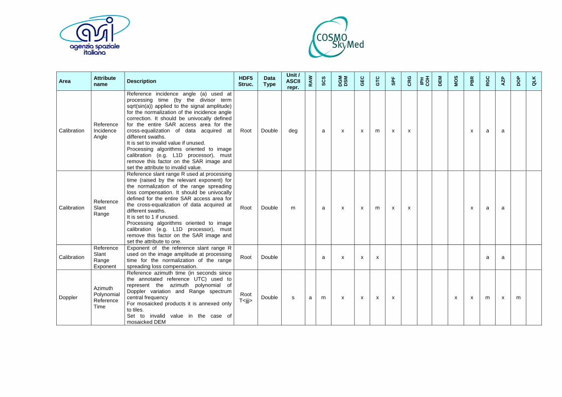
Area Attribute name Description HDF5
Struc. Data Type
Unit /ASCII repr. R
AW
SCS
DG
M
DSM
GEC
GTC
SPF
CR
G
IPH
C
OH
DEM
MO
S
PBR
RG
C
AZP
DO
P
QLK
Calibration Reference Incidence Angle
Reference incidence angle (a) used at processing time (by the divisor term sqrt(sin(a)) applied to the signal amplitude) for the normalization of the incidence angle correction. It should be univocally defined for the entire SAR access area for the cross-equalization of data acquired at different swaths. It is set to invalid value if unused. Processing algorithms oriented to image calibration (e.g. L1D processor), must remove this factor on the SAR image and set the attribute to invalid value.
Root Double deg a x x m x x x a a
Calibration Reference Slant Range
Reference slant range R used at processing time (raised by the relevant exponent) for the normalization of the range spreading loss compensation. It should be univocally defined for the entire SAR access area for the cross-equalization of data acquired at different swaths. It is set to 1 if unused. Processing algorithms oriented to image calibration (e.g. L1D processor), must remove this factor on the SAR image and set the attribute to one.
Root Double m a x x m x x x a a
Calibration
Reference Slant Range Exponent
Exponent of the reference slant range R used on the image amplitude at processing time for the normalization of the range spreading loss compensation.
Root Double a x x x a a
Doppler
Azimuth Polynomial Reference Time
Reference azimuth time (in seconds since the annotated reference UTC) used to represent the azimuth polynomial of Doppler variation and Range spectrum central frequency For mosaicked products it is annexed only to tiles. Set to invalid value in the case of mosaicked DEM
Root T<jjj> Double s a m x x x x x x m x m
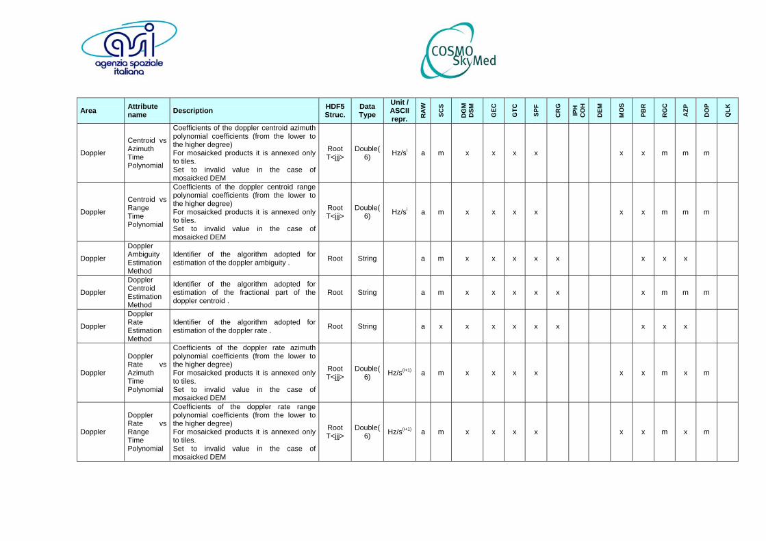
Area Attribute name Description HDF5
Struc. Data Type
Unit /ASCII repr. R
AW
SCS
DG
M
DSM
GEC
GTC
SPF
CR
G
IPH
C
OH
DEM
MO
S
PBR
RG
C
AZP
DO
P
QLK
Doppler
Centroid vs Azimuth Time Polynomial
Coefficients of the doppler centroid azimuth polynomial coefficients (from the lower to the higher degree) For mosaicked products it is annexed only to tiles. Set to invalid value in the case of mosaicked DEM
Root T<jjj>
Double(6) Hz/si a m x x x x x x m m m
Doppler
Centroid vs Range Time Polynomial
Coefficients of the doppler centroid range polynomial coefficients (from the lower to the higher degree) For mosaicked products it is annexed only to tiles. Set to invalid value in the case of mosaicked DEM
Root T<jjj>
Double(6) Hz/si a m x x x x x x m m m
Doppler
Doppler Ambiguity Estimation Method
Identifier of the algorithm adopted for estimation of the doppler ambiguity . Root String a m x x x x x x x x
Doppler
Doppler Centroid Estimation Method
Identifier of the algorithm adopted for estimation of the fractional part of the doppler centroid .
Root String a m x x x x x x m m m
Doppler
Doppler Rate Estimation Method
Identifier of the algorithm adopted for estimation of the doppler rate . Root String a x x x x x x x x x
Doppler
Doppler Rate vs Azimuth Time Polynomial
Coefficients of the doppler rate azimuth polynomial coefficients (from the lower to the higher degree) For mosaicked products it is annexed only to tiles. Set to invalid value in the case of mosaicked DEM
Root T<jjj>
Double(6) Hz/s(i+1) a m x x x x x x m x m
Doppler
Doppler Rate vs Range Time Polynomial
Coefficients of the doppler rate range polynomial coefficients (from the lower to the higher degree) For mosaicked products it is annexed only to tiles. Set to invalid value in the case of mosaicked DEM
Root T<jjj>
Double(6) Hz/s(i+1) a m x x x x x x m x m
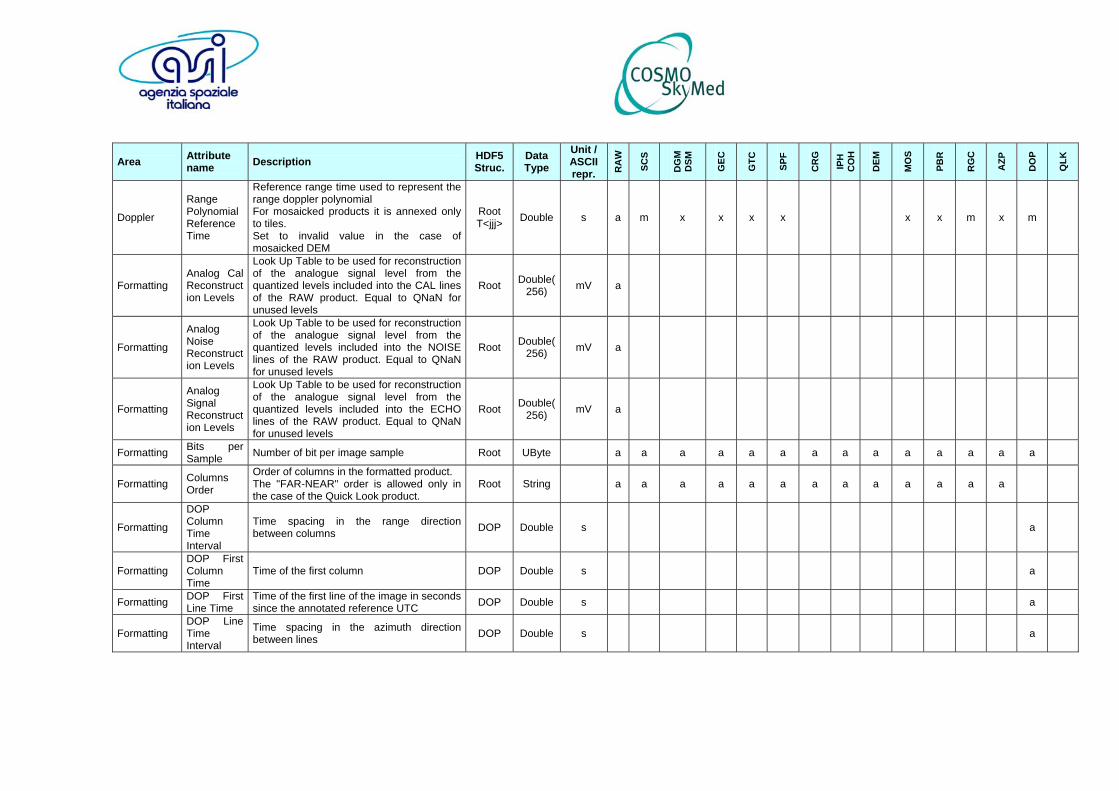
Area Attribute name Description HDF5
Struc. Data Type
Unit /ASCII repr. R
AW
SCS
DG
M
DSM
GEC
GTC
SPF
CR
G
IPH
C
OH
DEM
MO
S
PBR
RG
C
AZP
DO
P
QLK
Doppler
Range Polynomial Reference Time
Reference range time used to represent the range doppler polynomial For mosaicked products it is annexed only to tiles. Set to invalid value in the case of mosaicked DEM
Root T<jjj> Double s a m x x x x x x m x m
Formatting Analog Cal Reconstruction Levels
Look Up Table to be used for reconstruction of the analogue signal level from the quantized levels included into the CAL lines of the RAW product. Equal to QNaN for unused levels
Root Double(256) mV a
Formatting
Analog Noise Reconstruction Levels
Look Up Table to be used for reconstruction of the analogue signal level from the quantized levels included into the NOISE lines of the RAW product. Equal to QNaN for unused levels
Root Double(256) mV a
Formatting
Analog Signal Reconstruction Levels
Look Up Table to be used for reconstruction of the analogue signal level from the quantized levels included into the ECHO lines of the RAW product. Equal to QNaN for unused levels
Root Double(256) mV a
Formatting Bits per Sample Number of bit per image sample Root UByte a a a a a a a a a a a a a a
Formatting Columns Order
Order of columns in the formatted product. The "FAR-NEAR" order is allowed only in the case of the Quick Look product.
Root String a a a a a a a a a a a a a
Formatting
DOP Column Time Interval
Time spacing in the range direction between columns DOP Double s a
Formatting DOP First Column Time
Time of the first column DOP Double s a
Formatting DOP First Line Time
Time of the first line of the image in seconds since the annotated reference UTC DOP Double s a
Formatting DOP Line Time Interval
Time spacing in the azimuth direction between lines DOP Double s a

Area Attribute name Description HDF5
Struc. Data Type
Unit /ASCII repr. R
AW
SCS
DG
M
DSM
GEC
GTC
SPF
CR
G
IPH
C
OH
DEM
MO
S
PBR
RG
C
AZP
DO
P
QLK
Formatting
Equivalent Column Time Interval
Equivalent time spacing in the range direction between columns S<mm> Double s a m m
Formatting
Equivalent First Column Time
Equivalent time of the first column of the data in seconds. If set to QNaN it indicates that the compensation of SWST change has not been performed and the attribute "Range First Times" must be considered. In the case of burst mode data, it is set to the minimum of the equivalent times of the bursts included into the subswath
S<mm> Double s a m m
Formatting Equivalent First Line Time
Equivalent time of the first line of the data in seconds since the annotated reference UTC. In the case of burst mode data, it is set to the equivalent time of the first burst included into the subswath
S<mm> Double s a m m
Formatting Equivalent Line Time Interval
Equivalent time spacing in the azimuth direction between lines S<mm> Double s a m m
Formatting Image Layers Number of Image Layers Root UByte a x x x x x x x x x x x x
Formatting Image Scale Scale used for image representation Root String a a a a a a a a a a a a a
Formatting Layover Pixel Value
Value used for representation of pixels in layover geometry GIM Short a
Formatting Lines Order Order of lines in the formatted product. The "LATE-EARLY" order is allowed only in the case of the Quick Look product.
Root String a a a a a a a a a a a a a
Formatting
Master Zero Doppler Azimuth First Time
Time of the first line of the ot the input master image to interferometry
SBI MBI Double s a x
Formatting
Master Zero Doppler Azimuth Last Time
Time of the last line of the ot the input master image to interferometry
SBI MBI Double s a x

Area Attribute name Description HDF5
Struc. Data Type
Unit /ASCII repr. R
AW
SCS
DG
M
DSM
GEC
GTC
SPF
CR
G
IPH
C
OH
DEM
MO
S
PBR
RG
C
AZP
DO
P
QLK
Formatting
Master Zero Doppler Range First Time
Time of the first column of the ot the input master image to interferometry
SBI MBI Double s a x
Formatting
Master Zero Doppler Range Last Time
Time of the last column of the ot the input master image to interferometry
SBI MBI Double s a x
Formatting
Original Zero Doppler Azimuth First Time
Time of the first line of the input image (master/slave), before coregistration
SBI MBI Double s a
Formatting
Original Zero Doppler Azimuth Last Time
Time of the last line of the input image (master/slave), before coregistration
SBI MBI Double s a
Formatting
Original Zero Doppler Range First Time
Time of the first column of the input image (master/slave), before coregistration
SBI MBI Double s a
Formatting
Original Zero Doppler Range Last Time
Time of the last column of the input image (master/slave), before coregistration
SBI MBI Double s a
Formatting Quick Look Columns Order
Order of columns in the quick look layer. For quick look annexed to Level 0 product, it is conditioned by the consideration about geometric representation of the Quick Look product (see "Higher Level Products for Civilian Application: Products Specification" for details) aiming to simplify the image intepretation. For other products, it inherits the order of the full resolution layer.
QLK String a a a a a a a a a a a x

Area Attribute name Description HDF5
Struc. Data Type
Unit /ASCII repr. R
AW
SCS
DG
M
DSM
GEC
GTC
SPF
CR
G
IPH
C
OH
DEM
MO
S
PBR
RG
C
AZP
DO
P
QLK
Formatting Quick Look Lines Order
Order of lines in the quick look layer. For quick look annexed to Level 0 product, it is conditioned by the consideration about geometric representation of the Quick Look product (see "Higher Level Products for Civilian Application: Products Specification" for details) aiming to simplify the image intepretation. For other products, it inherits the order of the full resolution layer.
QLK String a a a a a a a a a a a x
Formatting Sample Format Sample data type Root String a a a a a a a a a a a a a a
Formatting Samples per Pixel Number of samples per pixels Root UByte a a a a a a a a a a a a a a
Formatting Shadowing Pixel Value
Value used for representation of pixels in shadowing geometry GIM Short a
Formatting
SIM Column Time Interval
Time spacing in the range direction between columns Root Double s
Formatting SIM First Column Time
Time of the first column Root Double s
Formatting SIM First Line Time
Time of the first line of the image in seconds since the annotated reference UTC Root Double s
Formatting SIM Line Time Interval
Time spacing in the azimuth direction between lines Root Double s
Formatting
Slave Zero Doppler Azimuth First Time
Time of the first line of the ot the input slave image to interferometry
SBI MBI Double s a x
Formatting
Slave Zero Doppler Azimuth Last Time
Time of the last line of the ot the input slave image to interferometry
SBI MBI Double s a x
Formatting
Slave Zero Doppler Range First Time
Time of the first column of the ot the input slave image to interferometry
SBI MBI Double s a x
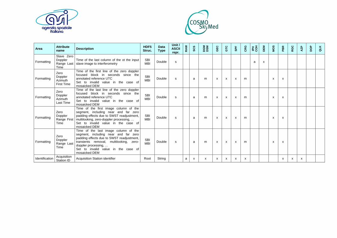
Area Attribute name Description HDF5
Struc. Data Type
Unit /ASCII repr. R
AW
SCS
DG
M
DSM
GEC
GTC
SPF
CR
G
IPH
C
OH
DEM
MO
S
PBR
RG
C
AZP
DO
P
QLK
Formatting
Slave Zero Doppler Range Last Time
Time of the last column of the ot the input slave image to interferometry
SBI MBI Double s a x
Formatting
Zero Doppler Azimuth First Time
Time of the first line of the zero doppler focused block in seconds since the annotated reference UTC Set to invalid value in the case of mosaicked DEM
SBI MBI Double s a m x x x m x x
Formatting
Zero Doppler Azimuth Last Time
Time of the last line of the zero doppler focused block in seconds since the annotated reference UTC Set to invalid value in the case of mosaicked DEM
SBI MBI Double s a m x x x m x x
Formatting
Zero Doppler Range First Time
Time of the first image column of the segment, including near and far zero padding effects due to SWST readjustment, multilooking, zero-doppler processing, … Set to invalid value in the case of mosaicked DEM
SBI MBI Double s a m x x x m x x
Formatting
Zero Doppler Range Last Time
Time of the last image column of the segment, including near and far zero padding effects due to SWST readjustment, transients removal, multilooking, zero-doppler processing, … Set to invalid value in the case of mosaicked DEM
SBI MBI Double s a m x x x m x x
Identification Acquisition Station ID Acquisition Station identifier Root String a x x x x x x x x x

Area Attribute name Description HDF5
Struc. Data Type
Unit /ASCII repr. R
AW
SCS
DG
M
DSM
GEC
GTC
SPF
CR
G
IPH
C
OH
DEM
MO
S
PBR
RG
C
AZP
DO
P
QLK
Identification
AcquisitionStation
Acquisition Station code where product has been acquired from. Allowed values: 1100 1101 1200 1201 1300 1301 … See GS ICD [R3] Section 6.3.3
Root UInt 9 digits
x
Identification
BandReductionFlag
If True indicates that this ISF is acquired in SPOT300 Mode using the band reduction Allowed values: TRUE | FALSE Default FALSE
Root String
x
Identification CRG Image Flag
Flag indicating if the image has been used such as Master rather than Slave in co-registration process (both in master and slave images)
Root String a
Identification Delivery Mode
Identification of the processing mode used to meet the delivery time constraints. It is strictly related to the accuracy level of the support data (in partiular of the orbital data) used to originate the product
Root String a x x x x x x x x x
Identification Downlink Start UTC
Downlink time of the first echo line of the Level 0 file used as input to generate the product
Root String Epoch a x x x x x x x x x
Identification Downlink Stop UTC
Downlink time of the last echo line of the Level 0 file used as input to generate the product
Root String Epoch a x x x x x x x x x
IdentificationMaster Product Filename
Filename of the master product used as reference scene for coregistration. Equal to Product Filename in master one
Root String a
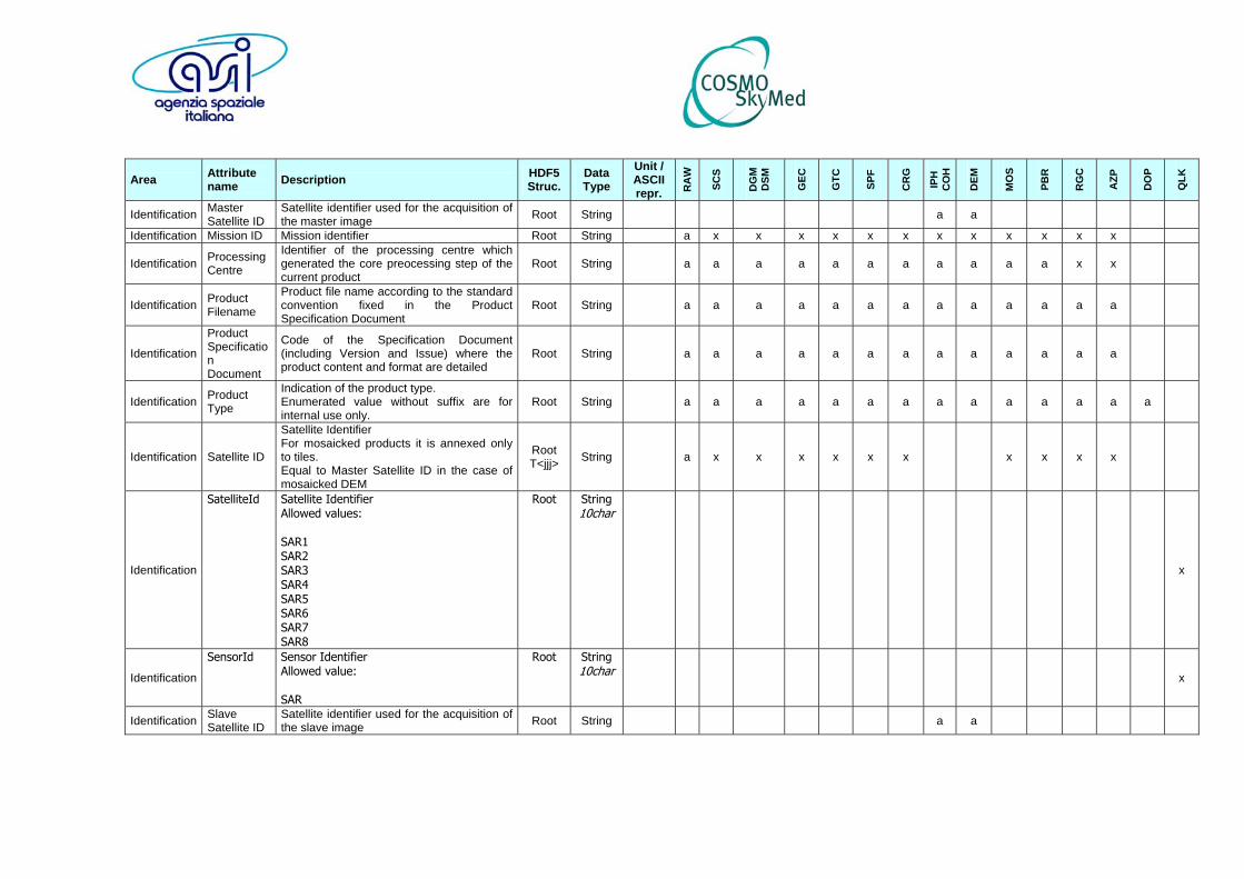
Area Attribute name Description HDF5
Struc. Data Type
Unit /ASCII repr. R
AW
SCS
DG
M
DSM
GEC
GTC
SPF
CR
G
IPH
C
OH
DEM
MO
S
PBR
RG
C
AZP
DO
P
QLK
Identification Master Satellite ID
Satellite identifier used for the acquisition of the master image Root String a a
Identification Mission ID Mission identifier Root String a x x x x x x x x x x x x
Identification Processing Centre
Identifier of the processing centre which generated the core preocessing step of the current product
Root String a a a a a a a a a a a x x
Identification Product Filename
Product file name according to the standard convention fixed in the Product Specification Document
Root String a a a a a a a a a a a a a
Identification
Product Specification Document
Code of the Specification Document (including Version and Issue) where the product content and format are detailed
Root String a a a a a a a a a a a a a
Identification Product Type
Indication of the product type. Enumerated value without suffix are for internal use only.
Root String a a a a a a a a a a a a a a
Identification Satellite ID
Satellite Identifier For mosaicked products it is annexed only to tiles. Equal to Master Satellite ID in the case of mosaicked DEM
Root T<jjj> String a x x x x x x x x x x
Identification
SatelliteId Satellite Identifier Allowed values: SAR1 SAR2 SAR3 SAR4 SAR5 SAR6 SAR7 SAR8
Root String 10char
x
Identification
SensorId Sensor Identifier Allowed value: SAR
Root String 10char
x
Identification Slave Satellite ID
Satellite identifier used for the acquisition of the slave image Root String a a
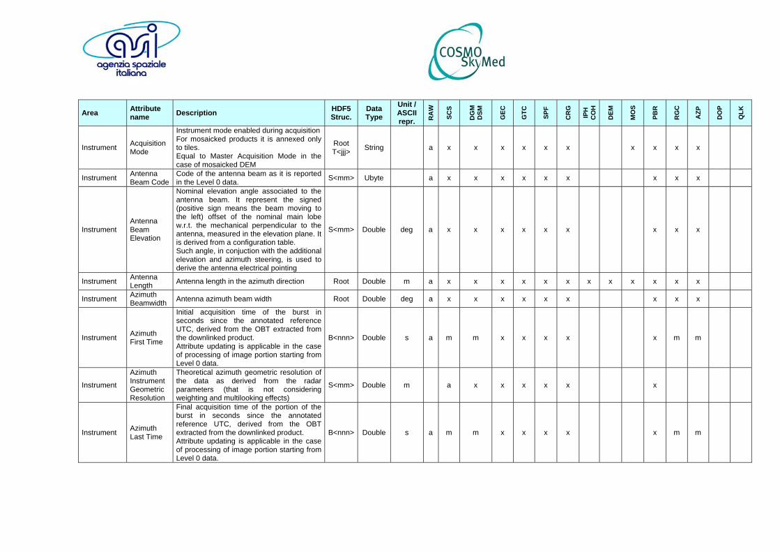
Area Attribute name Description HDF5
Struc. Data Type
Unit /ASCII repr. R
AW
SCS
DG
M
DSM
GEC
GTC
SPF
CR
G
IPH
C
OH
DEM
MO
S
PBR
RG
C
AZP
DO
P
QLK
Instrument Acquisition Mode
Instrument mode enabled during acquisitionFor mosaicked products it is annexed only to tiles. Equal to Master Acquisition Mode in the case of mosaicked DEM
Root T<jjj> String a x x x x x x x x x x
Instrument Antenna Beam Code
Code of the antenna beam as it is reported in the Level 0 data. S<mm> Ubyte a x x x x x x x x x
Instrument Antenna Beam Elevation
Nominal elevation angle associated to the antenna beam. It represent the signed (positive sign means the beam moving to the left) offset of the nominal main lobe w.r.t. the mechanical perpendicular to the antenna, measured in the elevation plane. It is derived from a configuration table. Such angle, in conjuction with the additional elevation and azimuth steering, is used to derive the antenna electrical pointing
S<mm> Double deg a x x x x x x x x x
Instrument Antenna Length Antenna length in the azimuth direction Root Double m a x x x x x x x x x x x x
Instrument Azimuth Beamwidth Antenna azimuth beam width Root Double deg a x x x x x x x x x
Instrument Azimuth First Time
Initial acquisition time of the burst in seconds since the annotated reference UTC, derived from the OBT extracted from the downlinked product. Attribute updating is applicable in the case of processing of image portion starting from Level 0 data.
B<nnn> Double s a m m x x x x x m m
Instrument
Azimuth Instrument Geometric Resolution
Theoretical azimuth geometric resolution of the data as derived from the radar parameters (that is not considering weighting and multilooking effects)
S<mm> Double m a x x x x x x
Instrument Azimuth Last Time
Final acquisition time of the portion of the burst in seconds since the annotated reference UTC, derived from the OBT extracted from the downlinked product. Attribute updating is applicable in the case of processing of image portion starting from Level 0 data.
B<nnn> Double s a m m x x x x x m m
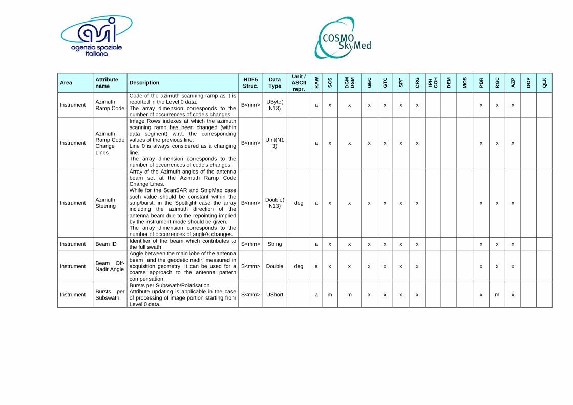
Area Attribute name Description HDF5
Struc. Data Type
Unit /ASCII repr. R
AW
SCS
DG
M
DSM
GEC
GTC
SPF
CR
G
IPH
C
OH
DEM
MO
S
PBR
RG
C
AZP
DO
P
QLK
Instrument Azimuth Ramp Code
Code of the azimuth scanning ramp as it is reported in the Level 0 data. The array dimension corresponds to the number of occurrences of code's changes.
B<nnn> UByte(N13) a x x x x x x x x x
Instrument
Azimuth Ramp Code Change Lines
Image Rows indexes at which the azimuth scanning ramp has been changed (within data segment) w.r.t. the corresponding values of the previous line. Line 0 is always considered as a changing line. The array dimension corresponds to the number of occurrences of code's changes.
B<nnn> UInt(N13) a x x x x x x x x x
Instrument Azimuth Steering
Array of the Azimuth angles of the antenna beam set at the Azimuth Ramp Code Change Lines. While for the ScanSAR and StripMap case such value should be constant within the strip/burst, in the Spotlight case the array including the azimuth direction of the antenna beam due to the repointing implied by the instrument mode should be given. The array dimension corresponds to the number of occurrences of angle's changes.
B<nnn> Double(N13) deg a x x x x x x x x x
Instrument Beam ID Identifier of the beam which contributes to the full swath S<mm> String a x x x x x x x x x
Instrument Beam Off-Nadir Angle
Angle between the main lobe of the antenna beam and the geodetic nadir, measured in acquisition geometry. It can be used for a coarse approach to the antenna pattern compensation.
S<mm> Double deg a x x x x x x x x x
Instrument Bursts per Subswath
Bursts per Subswath/Polarisation. Attribute updating is applicable in the case of processing of image portion starting from Level 0 data.
S<mm> UShort a m m x x x x x m x
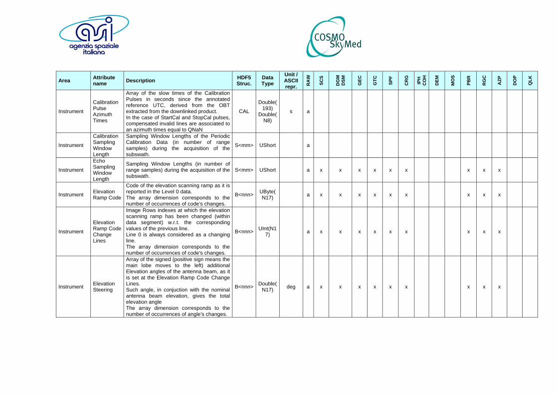
Area Attribute name Description HDF5
Struc. Data Type
Unit /ASCII repr. R
AW
SCS
DG
M
DSM
GEC
GTC
SPF
CR
G
IPH
C
OH
DEM
MO
S
PBR
RG
C
AZP
DO
P
QLK
Instrument
Calibration Pulse Azimuth Times
Array of the slow times of the Calibration Pulses in seconds since the annotated reference UTC, derived from the OBT extracted from the downlinked product. In the case of StartCal and StopCal pulses, compensated invalid lines are associated to an azimuth times equal to QNaN
CAL
Double(193)
Double(N8)
s a
Instrument
Calibration Sampling Window Length
Sampling Window Lengths of the Periodic Calibration Data (in number of range samples) during the acquisition of the subswath.
S<mm> UShort a
Instrument
Echo Sampling Window Length
Sampling Window Lengths (in number of range samples) during the acquisition of the subswath.
S<mm> UShort a x x x x x x x x x
Instrument Elevation Ramp Code
Code of the elevation scanning ramp as it is reported in the Level 0 data. The array dimension corresponds to the number of occurrences of code's changes.
B<nnn> UByte(N17) a x x x x x x x x x
Instrument
Elevation Ramp Code Change Lines
Image Rows indexes at which the elevation scanning ramp has been changed (within data segment) w.r.t. the corresponding values of the previous line. Line 0 is always considered as a changing line. The array dimension corresponds to the number of occurrences of code's changes.
B<nnn> UInt(N17) a x x x x x x x x x
Instrument Elevation Steering
Array of the signed (positive sign means the main lobe moves to the left) additional Elevation angles of the antenna beam, as it is set at the Elevation Ramp Code Change Lines. Such angle, in conjuction with the nominal antenna beam elevation, gives the total elevation angle The array dimension corresponds to the number of occurrences of angle's changes.
B<nnn> Double(N17) deg a x x x x x x x x x
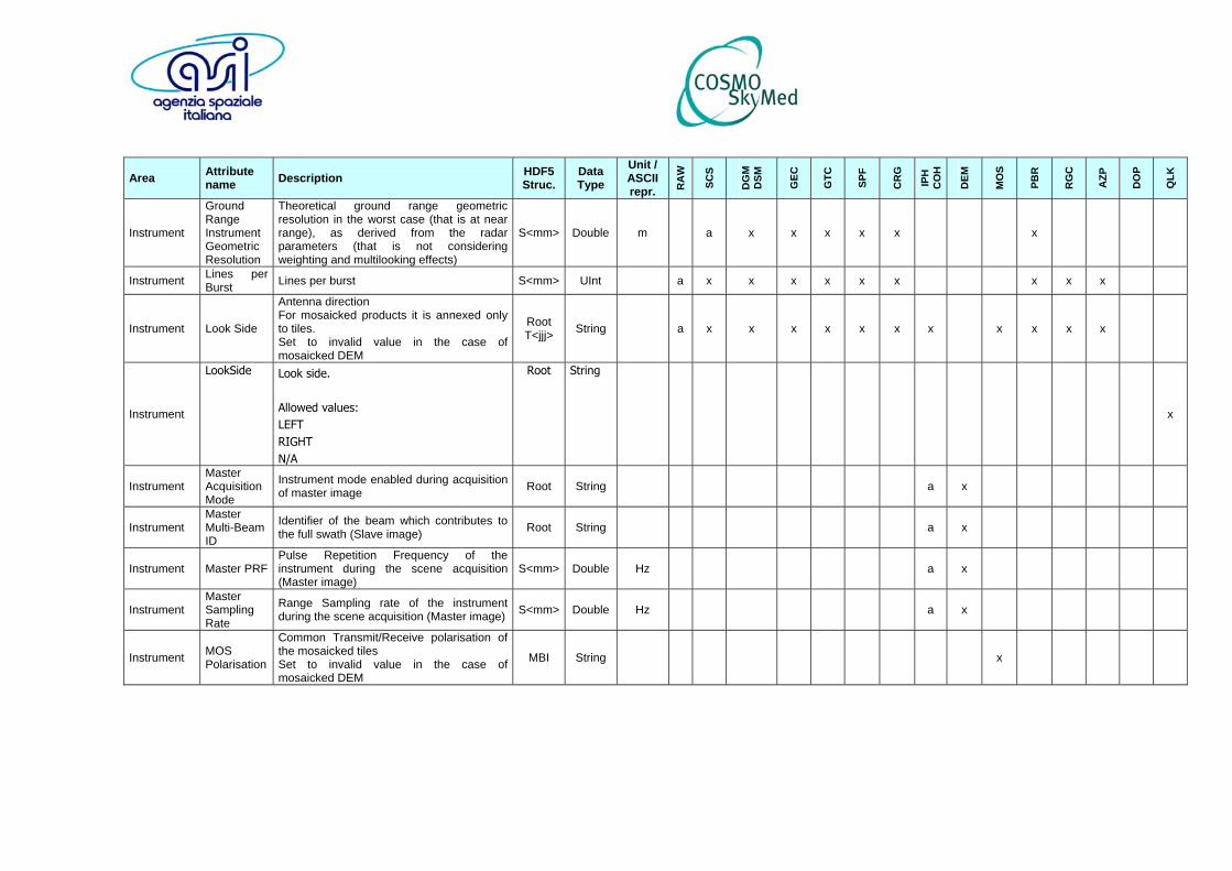
Area Attribute name Description HDF5
Struc. Data Type
Unit /ASCII repr. R
AW
SCS
DG
M
DSM
GEC
GTC
SPF
CR
G
IPH
C
OH
DEM
MO
S
PBR
RG
C
AZP
DO
P
QLK
Instrument
Ground Range Instrument Geometric Resolution
Theoretical ground range geometric resolution in the worst case (that is at near range), as derived from the radar parameters (that is not considering weighting and multilooking effects)
S<mm> Double m a x x x x x x
Instrument Lines per Burst Lines per burst S<mm> UInt a x x x x x x x x x
Instrument Look Side
Antenna direction For mosaicked products it is annexed only to tiles. Set to invalid value in the case of mosaicked DEM
Root T<jjj> String a x x x x x x x x x x x
Instrument
LookSide Look side. Allowed values: LEFT RIGHT N/A
Root String
x
Instrument Master Acquisition Mode
Instrument mode enabled during acquisition of master image Root String a x
Instrument Master Multi-Beam ID
Identifier of the beam which contributes to the full swath (Slave image) Root String a x
Instrument Master PRF Pulse Repetition Frequency of the instrument during the scene acquisition (Master image)
S<mm> Double Hz a x
Instrument Master Sampling Rate
Range Sampling rate of the instrument during the scene acquisition (Master image) S<mm> Double Hz a x
Instrument MOS Polarisation
Common Transmit/Receive polarisation of the mosaicked tiles Set to invalid value in the case of mosaicked DEM
MBI String x
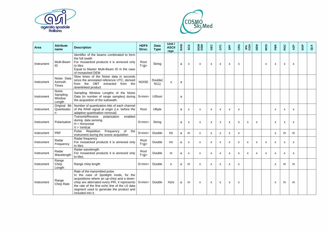
Area Attribute name Description HDF5
Struc. Data Type
Unit /ASCII repr. R
AW
SCS
DG
M
DSM
GEC
GTC
SPF
CR
G
IPH
C
OH
DEM
MO
S
PBR
RG
C
AZP
DO
P
QLK
Instrument Multi-Beam ID
Identifier of the beams combinated to form the full swath For mosaicked products it is annexed only to tiles. Equal to Master Multi-Beam ID in the case of mosaicked DEM
Root T<jjj> String a x x x x x x x x x x
Instrument Noise Data Azimuth Times
Slow times of the Noise data in seconds since the annotated reference UTC, derived from the OBT extracted from the downlinked product
NOISE Double(N11) s a
Instrument
Noise Sampling Window Length
Sampling Window Lengths of the Noise Data (in number of range samples) during the acquisition of the subswath.
S<mm> UShort a
Instrument Original Bit Quantisation
Number of quantization bits of each channel of the RAW signal at origin (i.e. before the adaptive quantisation removal)
Root UByte a x x x x x x x x x
Instrument Polarisation
Transmit/Receive polarisation enabled during data sensing. H = Horizontal V = Vertical
S<mm> String a x x x x x x x x x x x
Instrument PRF Pulse Repetition Frequency of the instrument during the scene acquisition S<mm> Double Hz a m x x x x x x m m
Instrument Radar Frequency
Radar frequency For mosaicked products it is annexed only to tiles.
Root T<jjj> Double Hz a x x x x x x x x x x x x
Instrument Radar Wavelength
Radar wavelength For mosaicked products it is annexed only to tiles.
Root T<jjj> Double m a x x x x x x x x x x x x
Instrument Range Chirp Length
Range chirp length S<mm> Double s a m x x x x x x m m
Instrument Range Chirp Rate
Rate of the transmitted pulse. In the case of Spotlight mode, for the acquisitions where an up-chirp and a down-chirp are alternated every PRI, it represents the rate of the first echo line of the L0 data segment used to generate the product and included into it.
S<mm> Double Hz/s a m x x x x x x m m
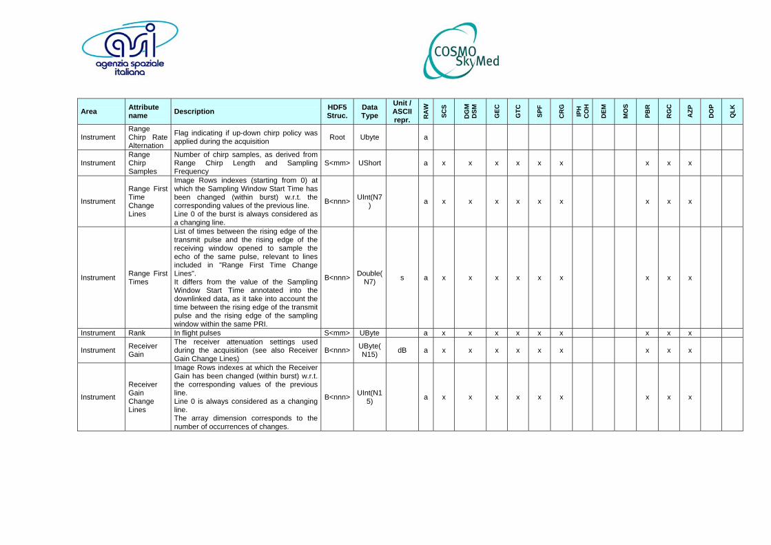
Area Attribute name Description HDF5
Struc. Data Type
Unit /ASCII repr. R
AW
SCS
DG
M
DSM
GEC
GTC
SPF
CR
G
IPH
C
OH
DEM
MO
S
PBR
RG
C
AZP
DO
P
QLK
Instrument Range Chirp Rate Alternation
Flag indicating if up-down chirp policy was applied during the acquisition Root Ubyte a
Instrument Range Chirp Samples
Number of chirp samples, as derived from Range Chirp Length and Sampling Frequency
S<mm> UShort a x x x x x x x x x
Instrument
Range First Time Change Lines
Image Rows indexes (starting from 0) at which the Sampling Window Start Time has been changed (within burst) w.r.t. the corresponding values of the previous line. Line 0 of the burst is always considered as a changing line.
B<nnn> UInt(N7) a x x x x x x x x x
Instrument Range First Times
List of times between the rising edge of the transmit pulse and the rising edge of the receiving window opened to sample the echo of the same pulse, relevant to lines included in "Range First Time Change Lines". It differs from the value of the Sampling Window Start Time annotated into the downlinked data, as it take into account the time between the rising edge of the transmit pulse and the rising edge of the sampling window within the same PRI.
B<nnn> Double(N7) s a x x x x x x x x x
Instrument Rank In flight pulses S<mm> UByte a x x x x x x x x x
Instrument Receiver Gain
The receiver attenuation settings used during the acquisition (see also Receiver Gain Change Lines)
B<nnn> UByte(N15) dB a x x x x x x x x x
Instrument
Receiver Gain Change Lines
Image Rows indexes at which the Receiver Gain has been changed (within burst) w.r.t. the corresponding values of the previous line. Line 0 is always considered as a changing line. The array dimension corresponds to the number of occurrences of changes.
B<nnn> UInt(N15) a x x x x x x x x x
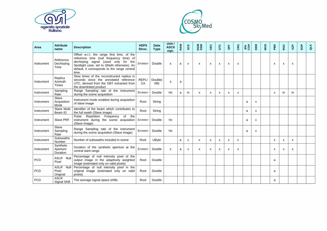
Area Attribute name Description HDF5
Struc. Data Type
Unit /ASCII repr. R
AW
SCS
DG
M
DSM
GEC
GTC
SPF
CR
G
IPH
C
OH
DEM
MO
S
PBR
RG
C
AZP
DO
P
QLK
Instrument Reference Dechirping Time
Offset w.r.t. the range first time, of the reference time (null frequency time) of dechirping signal (used only for the Spotlight case, set to QNaN otherwise). As default, it corresponds to the range central time.
S<mm> Double s a x x x x x x x x x
Instrument Replica Azimuth Times
Slow times of the reconstructed replica in seconds since the annotated reference UTC, derived from the OBT extracted from the downlinked product
REPLICA
Double(N8) s a
Instrument Sampling Rate
Range Sampling rate of the instrument during the scene acquisition S<mm> Double Hz a m x x x x x x m m
Instrument Slave Acquisition Mode
Instrument mode enabled during acquisition of slave image Root String a x
Instrument Slave Multi-Beam ID
Identifier of the beam which contributes to the full swath (Slave image) Root String a x
Instrument Slave PRF Pulse Repetition Frequency of the instrument during the scene acquisition (Slave Image)
S<mm> Double Hz a x
Instrument Slave Sampling Rate
Range Sampling rate of the instrument during the scene acquisition (Slave image) S<mm> Double Hz a x
Instrument Subswaths Number Number of subswaths included in scene Root UByte a x x x x x x x x x
Instrument Synthetic Aperture Duration
Duration of the synthetic aperture at the central slant range S<mm> Double s a x x x x x x x x x
PCD ASLR Null Pixel
Percentage of null intensity pixel of the output image in the adaptively weighted image (estimated only on valid pixels)
Root Double a
PCD ASLR Null Pixel Original
Percentage of null intensity pixel in the original Image (estimated only on valid pixels)
Root Double a
PCD ASLR Signal Shift The average signal space shifts Root Double a

Area Attribute name Description HDF5
Struc. Data Type
Unit /ASCII repr. R
AW
SCS
DG
M
DSM
GEC
GTC
SPF
CR
G
IPH
C
OH
DEM
MO
S
PBR
RG
C
AZP
DO
P
QLK
PCD
ASLR Signal to Clutter Ratio Mean
The average ratio of the weighted over the original Signal to Clutter Ratio Root Double a
PCD
ASLR Signal to Clutter Ratio Standard Deviation
The standard deviation of the ratio of the weighted over the original Signal to Clutter Ratio
Root Double a
PCD Attitude Product Category
Type of Attitude product used for processing. DOWNLINKED indicates the attitude data annexed to the Level 0 data as they are downlinked from the spacecraft RESTITUTED indicates the attitude data obtained by on-ground postprocessing. For mosaicked products it is annexed only to tiles.
Root T<jjj> String a x x m m x x x x x x
PCD
Central Range Frequency vs Azimuth Time Polynomial
Coefficients of the polynomial representing the variation (w.r.t. the relative azimuth times) of the central frequency of the range spectrum in the azimuth direction (from the lower to the higher degree). Annotated only in complex products. Not estimated (hence set to QNaN) in the case of intermediate products.
S<mm> Double(3) Hz/si a x x
PCD CRG Baseline
For each slave: Baseline orthogonal and parallel components w.r.t. the line of sight estimated at the image center Set to invalid value in Master Set to invalid valut in mosaiked products not representing a DEM
SBI MBI
T<jjj>
Double[2] m a x x x
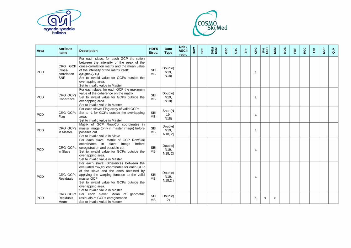
Area Attribute name Description HDF5
Struc. Data Type
Unit /ASCII repr. R
AW
SCS
DG
M
DSM
GEC
GTC
SPF
CR
G
IPH
C
OH
DEM
MO
S
PBR
RG
C
AZP
DO
P
QLK
PCD
CRG GCP Cross-correlation SNR
For each slave: for each GCP the ration between the intensity of the peak of the cross-correlation matrix and the mean value of the intensity of the matrix itself: qi=Ii(max)/<Ii>. Set to invalid value for GCPs outside the overlapping area. Set to invalid value in Master
SBI MBI
Double(N19, N18)
a
PCD CRG GCPs Coherence
For each slave: for each GCP the maximum value of the coherence on the matrix Set to invalid value for GCPs outside the overlapping area. Set to invalid value in Master
SBI MBI
Double(N19, N18)
a
PCD CRG GCPs Flag
For each slave: Flag array of valid GCPs Set to -1 for GCPs outside the overlapping area. Set to invalid value in Master
SBI MBI
Short(N19,
N18) a
PCD CRG GCPs in Master
Matrix of GCP Row/Col coordinates in master image (only in master image) before possible cut Set to invalid value in Slave
SBI MBI
Double[N19,
N18, 2] a
PCD CRG GCPs in Slave
For each slave: Matrix of GCP Row/Col coordinates in slave image before coregistration and possible cut Set to invalid value for GCPs outside the overlapping area. Set to invalid value in Master
SBI MBI
Double[N19,
N18, 2] a
PCD CRG GCPs Residuals
For each slave: Differences between the evaluated row,col coordinates for each GCP of the slave and the ones obtained by applying the warping function to the valid master GCP Set to invalid value for GCPs outside the overlapping area. Set to invalid value in Master
SBI MBI
Double(N19,
N18,2 ) a
PCD CRG GCPs Residuals Mean
For each slave: Mean of geometric residuals of GCPs coregistration Set to invalid value in Master
SBI MBI
Double(2) a x x

Area Attribute name Description HDF5
Struc. Data Type
Unit /ASCII repr. R
AW
SCS
DG
M
DSM
GEC
GTC
SPF
CR
G
IPH
C
OH
DEM
MO
S
PBR
RG
C
AZP
DO
P
QLK
PCD
CRG GCPs Residuals Standard Deviation
For each slave: Standard deviation of geometric residuals of GCPs coregistrationSet to invalid value in Master
SBI MBI
Double(2) a x x
PCD
CRG Master to Slave Warp Matrix
For each slave: Warp matrix converting master Row/Col indexes to the slave's ones in Coregistration process. Array is always dimensioned to represent a 3rd degree warp transformation; some field could be set to zero as function of the degree actually used. If R and C (resp. R' and C') represent Row-Col indexes in the master (resp. slave) reference, the first row of the matrix includes coefficients ai (i=0, ..., 9) such thatR' = a0 + a1*R + a2*C + a3*R^2 + a4*R*C + a5*C^2 + a6*R^3 + a7*R^2*C + a8*R*C^2 + a9*C^3 The second row of the matrix includes coefficients bi (i=0, ..., 9) such that C' = b0 + b1*R + b2*C + b3*R^2 + b4*R*C + b5*C^2 + b6*R^3 + b7*R^2*C + b8*R*C^2 + b9*C^3
SBI MBI
Double[2, 10] a
PCD
CRG Overlapping Percentage
For each slave: extension (as percentage of the master coverage) of the overlapping zone between the slave and the master Set to invalid value in Master
SBI MBI Double a
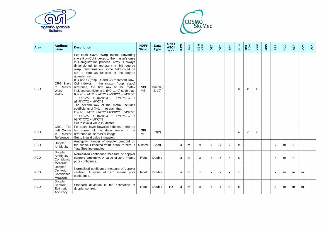
Area Attribute name Description HDF5
Struc. Data Type
Unit /ASCII repr. R
AW
SCS
DG
M
DSM
GEC
GTC
SPF
CR
G
IPH
C
OH
DEM
MO
S
PBR
RG
C
AZP
DO
P
QLK
PCD
CRG Slave to Master Warp Matrix
For each slave: Warp matrix converting slave Row/Col indexes to the master's ones in Coregistration process. Array is always dimensioned to represent a 3rd degree warp transformation; some field could be set to zero as function of the degree actually used. If R and C (resp. R' and C') represent Row-Col indexes in the master (resp. slave) reference, the first row of the matrix includes coefficients ai (i=0, ..., 9) such thatR = a0 + a1*R' + a2*C' + a3*R'^2 + a4*R'*C' + a5*C'^2 + a6*R'^3 + a7*R'^2*C' + a8*R'*C'^2 + a9*C'^3 The second row of the matrix includes coefficients bi (i=0, ..., 9) such that C = b0 + b1*R' + b2*C' + b3*R'^2 + b4*R'*C' + b5*C'^2 + b6*R'^3 + b7*R'^2*C' + b8*R'*C'^2 + b9*C'^3 Set to invalid value in Master
SBI MBI
Double[2, 10] a x x
PCD
CRG Top Left Corner in Master Reference
For each slave: Row/Col indexes of the top left corner of the slave image in the reference of the master image Set to invalid value in master.
SBI MBI Int(2) a x x
PCD Doppler Ambiguity
Ambiguity number of doppler centroid on the scene. Expected value equal to zero, if Yaw Steering enabled.
S<mm> Short a m x x x x x x m x
PCD
Doppler Ambiguity Confidence Measure
Normalized confidence measure of doppler centroid ambiguity. A value of zero means poor confidence.
Root Double a m x x x x x x m x
PCD
Doppler Centroid Confidence Measure
Normalized confidence measure of doppler centroid. A value of zero means poor confidence.
Root Double a m x x x x x x m m m
PCD
Doppler Centroid Estimation Accuracy
Standard deviation in the estimation of doppler centroid. Root Double Hz a m x x x x x x m m m
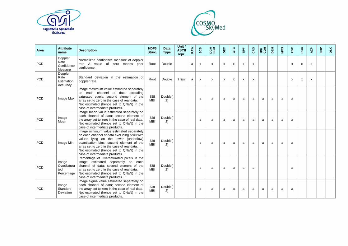
Area Attribute name Description HDF5
Struc. Data Type
Unit /ASCII repr. R
AW
SCS
DG
M
DSM
GEC
GTC
SPF
CR
G
IPH
C
OH
DEM
MO
S
PBR
RG
C
AZP
DO
P
QLK
PCD
Doppler Rate Confidence Measure
Normalized confidence measure of doppler rate A value of zero means poor confidence.
Root Double a x x x x x x x x x
PCD
Doppler Rate Estimation Accuracy
Standard deviation in the estimation of doppler rate. Root Double Hz/s a x x x x x x x x x
PCD Image Max
Image maximum value estimated separately on each channel of data excluding saturated pixels; second element of the array set to zero in the case of real data. Not estimated (hence set to QNaN) in the case of intermediate products.
SBI MBI
Double(2) a a a a a a a a a a
PCD Image Mean
Image mean value estimated separately on each channel of data; second element of the array set to zero in the case of real data.Not estimated (hence set to QNaN) in the case of intermediate products.
SBI MBI
Double(2) a a a a a a a a a a
PCD Image Min
Image minimum value estimated separately on each channel of data excluding pixel with values lying on the lower (underflow) quantisation bins; second element of the array set to zero in the case of real data. Not estimated (hence set to QNaN) in the case of intermediate products.
SBI MBI
Double(2) a a a a a a a a a a
PCD
Image OverSaturated Percentage
Percentage of Oversaturated pixels in the image estimated separately on each channel of data; second element of the array set to zero in the case of real data. Not estimated (hence set to QNaN) in the case of intermediate products.
SBI MBI
Double(2) a a a a a a a
PCD Image Standard Deviation
Image sigma value estimated separately on each channel of data; second element of the array set to zero in the case of real data.Not estimated (hence set to QNaN) in the case of intermediate products.
SBI MBI
Double(2) a a a a a a a a a a
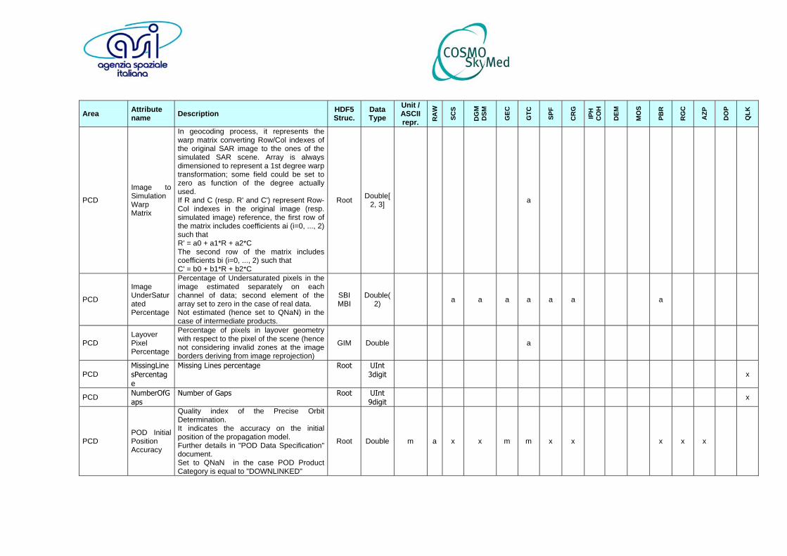
Area Attribute name Description HDF5
Struc. Data Type
Unit /ASCII repr. R
AW
SCS
DG
M
DSM
GEC
GTC
SPF
CR
G
IPH
C
OH
DEM
MO
S
PBR
RG
C
AZP
DO
P
QLK
PCD
Image to Simulation Warp Matrix
In geocoding process, it represents the warp matrix converting Row/Col indexes of the original SAR image to the ones of the simulated SAR scene. Array is always dimensioned to represent a 1st degree warp transformation; some field could be set to zero as function of the degree actually used. If R and C (resp. R' and C') represent Row-Col indexes in the original image (resp. simulated image) reference, the first row of the matrix includes coefficients ai (i=0, ..., 2) such that R' = a0 + a1*R + a2*C The second row of the matrix includes coefficients bi (i=0, ..., 2) such that C' = b0 + b1*R + b2*C
Root Double[2, 3] a
PCD
Image UnderSaturated Percentage
Percentage of Undersaturated pixels in the image estimated separately on each channel of data; second element of the array set to zero in the case of real data. Not estimated (hence set to QNaN) in the case of intermediate products.
SBI MBI
Double(2) a a a a a a a
PCD Layover Pixel Percentage
Percentage of pixels in layover geometry with respect to the pixel of the scene (hence not considering invalid zones at the image borders deriving from image reprojection)
GIM Double a
PCD MissingLinesPercentage
Missing Lines percentage Root UInt 3digit
x
PCD NumberOfGaps
Number of Gaps Root UInt 9digit
x
PCD POD Initial Position Accuracy
Quality index of the Precise Orbit Determination. It indicates the accuracy on the initial position of the propagation model. Further details in "POD Data Specification" document. Set to QNaN in the case POD Product Category is equal to "DOWNLINKED"
Root Double m a x x m m x x x x x

Area Attribute name Description HDF5
Struc. Data Type
Unit /ASCII repr. R
AW
SCS
DG
M
DSM
GEC
GTC
SPF
CR
G
IPH
C
OH
DEM
MO
S
PBR
RG
C
AZP
DO
P
QLK
PCD
POD Overlap Position Accuracy
Quality index of the Precise Orbit Determination. It indicates the accuracy of the platform position in the overlapping arcs. Further details in "POD Data Specification" document. Set to QNaN in the case POD Product Category is equal to "DOWNLINKED"
Root Double m a x x m m x x x x x
PCD POD Product Category
Quality index of the Precise Orbit Determination process. It indicates the level of accuracy of the orbital data annexed to the product. DOWNLINKED indicates the orbital data annexed to the Level 0 data as they are downlinked from the spacecraft PROPAGATED indicates the orbital data obtained by propagating restituted orbits after the end of the analyzed data arc FILTERED indicates the orbital data obtained by filtering the on board navigation solution RESTITUTED indicates the orbital data based on the GPS data acquired by on board GPS and the GPS ground network (CSK fiducial network and/or IGS network).Such attribute is strictly related to the product delivery mode (Fast Delivery rather than Standard Delivery). Fast Delivery mode implies usage of DOWNLINKED or PROPAGATED orbit Standard Delivery mode implies usage of FILTERED or RESTITUTED orbit For mosaicked products it is annexed only to tiles.
Root T<jjj> String a x x x x x x x x x x
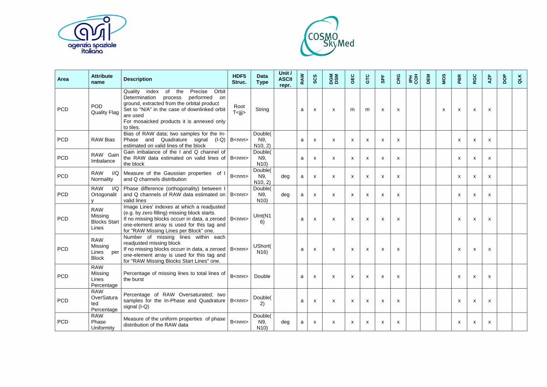
Area Attribute name Description HDF5
Struc. Data Type
Unit /ASCII repr. R
AW
SCS
DG
M
DSM
GEC
GTC
SPF
CR
G
IPH
C
OH
DEM
MO
S
PBR
RG
C
AZP
DO
P
QLK
PCD POD Quality Flag
Quality index of the Precise Orbit Determination process performed on ground, extracted from the orbital product Set to "N/A" in the case of downlinked orbit are used For mosaicked products it is annexed only to tiles.
Root T<jjj> String a x x m m x x x x x x
PCD RAW Bias Bias of RAW data; two samples for the In-Phase and Quadrature signal (I-Q) estimated on valid lines of the block
B<nnn>Double(
N9, N10, 2)
a x x x x x x x x x
PCD RAW Gain Imbalance
Gain imbalance of the I and Q channel of the RAW data estimated on valid lines of the block
B<nnn>Double(
N9, N10)
a x x x x x x x x x
PCD RAW I/Q Normality
Measure of the Gaussian properties of I and Q channels distribution B<nnn>
Double(N9,
N10, 2)deg a x x x x x x x x x
PCD RAW I/Q Ortogonality
Phase difference (orthogonality) between I and Q channels of RAW data estimated on valid lines
B<nnn>Double(
N9, N10)
deg a x x x x x x x x x
PCD
RAW Missing Blocks Start Lines
Image Lines' indexes at which a readjusted (e.g. by zero filling) missing block starts. If no missing blocks occurr in data, a zeroed one-element array is used for this tag and for "RAW Missing Lines per Block" one.
B<nnn> UInt(N16) a x x x x x x x x x
PCD
RAW Missing Lines per Block
Number of missing lines within each readjusted missing block If no missing blocks occurr in data, a zeroed one-element array is used for this tag and for "RAW Missing Blocks Start Lines" one.
B<nnn> UShort(N16) a x x x x x x x x x
PCD
RAW Missing Lines Percentage
Percentage of missing lines to total lines of the burst B<nnn> Double a x x x x x x x x x
PCD
RAW OverSaturated Percentage
Percentage of RAW Oversaturated; two samples for the In-Phase and Quadrature signal (I-Q)
B<nnn> Double(2) a x x x x x x x x x
PCD RAW Phase Uniformity
Measure of the uniform properties of phase distribution of the RAW data B<nnn>
Double(N9,
N10) deg a x x x x x x x x x
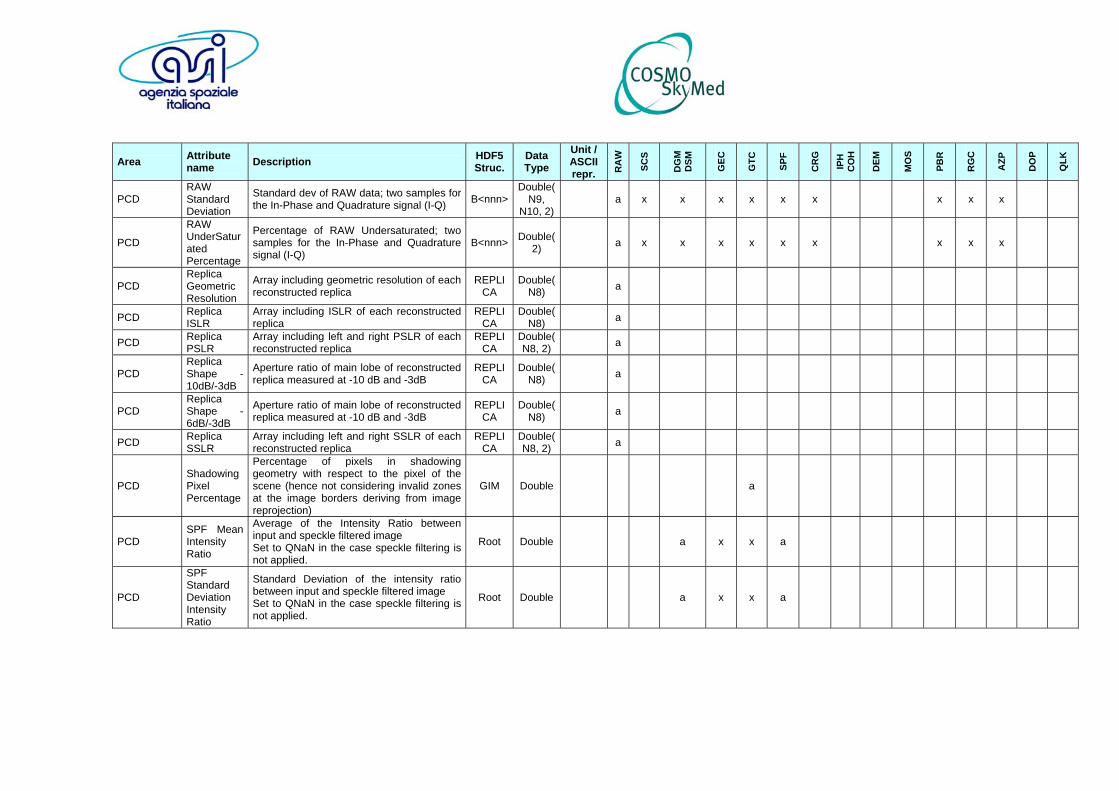
Area Attribute name Description HDF5
Struc. Data Type
Unit /ASCII repr. R
AW
SCS
DG
M
DSM
GEC
GTC
SPF
CR
G
IPH
C
OH
DEM
MO
S
PBR
RG
C
AZP
DO
P
QLK
PCD RAW Standard Deviation
Standard dev of RAW data; two samples for the In-Phase and Quadrature signal (I-Q) B<nnn>
Double(N9,
N10, 2) a x x x x x x x x x
PCD
RAW UnderSaturated Percentage
Percentage of RAW Undersaturated; two samples for the In-Phase and Quadrature signal (I-Q)
B<nnn> Double(2) a x x x x x x x x x
PCD Replica Geometric Resolution
Array including geometric resolution of each reconstructed replica
REPLICA
Double(N8) a
PCD Replica ISLR
Array including ISLR of each reconstructed replica
REPLICA
Double(N8) a
PCD Replica PSLR
Array including left and right PSLR of each reconstructed replica
REPLICA
Double(N8, 2) a
PCD Replica Shape -10dB/-3dB
Aperture ratio of main lobe of reconstructed replica measured at -10 dB and -3dB
REPLICA
Double(N8) a
PCD Replica Shape -6dB/-3dB
Aperture ratio of main lobe of reconstructed replica measured at -10 dB and -3dB
REPLICA
Double(N8) a
PCD Replica SSLR
Array including left and right SSLR of each reconstructed replica
REPLICA
Double(N8, 2) a
PCD Shadowing Pixel Percentage
Percentage of pixels in shadowing geometry with respect to the pixel of the scene (hence not considering invalid zones at the image borders deriving from image reprojection)
GIM Double a
PCD SPF Mean Intensity Ratio
Average of the Intensity Ratio between input and speckle filtered image Set to QNaN in the case speckle filtering is not applied.
Root Double a x x a
PCD
SPF Standard Deviation Intensity Ratio
Standard Deviation of the intensity ratio between input and speckle filtered image Set to QNaN in the case speckle filtering is not applied.
Root Double a x x a
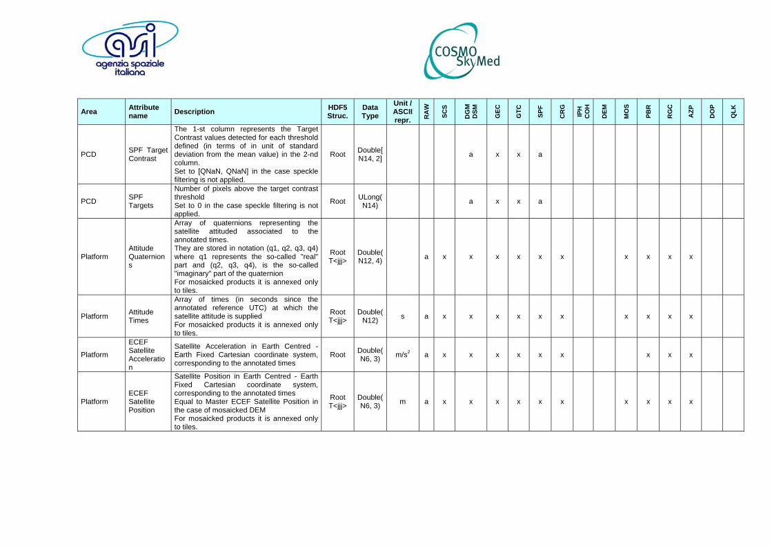
Area Attribute name Description HDF5
Struc. Data Type
Unit /ASCII repr. R
AW
SCS
DG
M
DSM
GEC
GTC
SPF
CR
G
IPH
C
OH
DEM
MO
S
PBR
RG
C
AZP
DO
P
QLK
PCD SPF Target Contrast
The 1-st column represents the Target Contrast values detected for each threshold defined (in terms of in unit of standard deviation from the mean value) in the 2-nd column. Set to [QNaN, QNaN] in the case speckle filtering is not applied.
Root Double[N14, 2] a x x a
PCD SPF Targets
Number of pixels above the target contrast threshold Set to 0 in the case speckle filtering is not applied.
Root ULong(N14) a x x a
Platform Attitude Quaternions
Array of quaternions representing the satellite attituded associated to the annotated times. They are stored in notation (q1, q2, q3, q4) where q1 represents the so-called "real" part and (q2, q3, q4), is the so-called "imaginary" part of the quaternion For mosaicked products it is annexed only to tiles.
Root T<jjj>
Double(N12, 4) a x x x x x x x x x x
Platform Attitude Times
Array of times (in seconds since the annotated reference UTC) at which the satellite attitude is supplied For mosaicked products it is annexed only to tiles.
Root T<jjj>
Double(N12) s a x x x x x x x x x x
Platform
ECEF Satellite Acceleration
Satellite Acceleration in Earth Centred - Earth Fixed Cartesian coordinate system, corresponding to the annotated times
Root Double(N6, 3) m/s2 a x x x x x x x x x
Platform ECEF Satellite Position
Satellite Position in Earth Centred - Earth Fixed Cartesian coordinate system, corresponding to the annotated times Equal to Master ECEF Satellite Position in the case of mosaicked DEM For mosaicked products it is annexed only to tiles.
Root T<jjj>
Double(N6, 3) m a x x x x x x x x x x
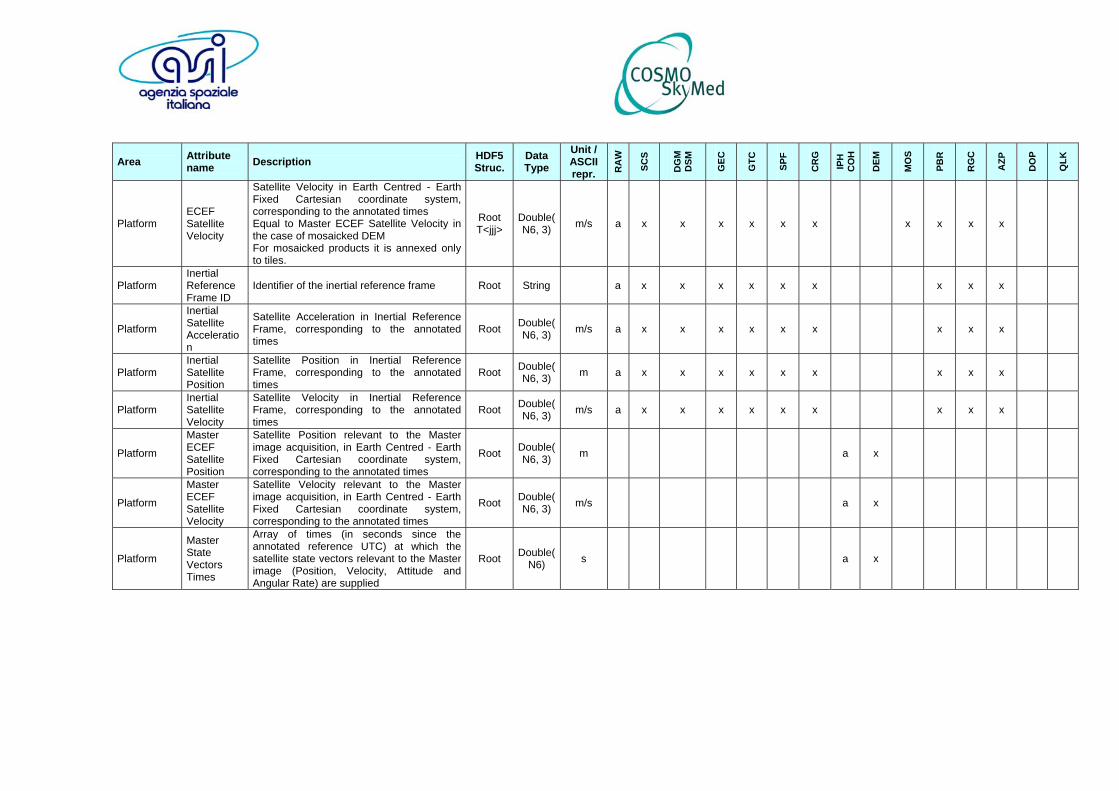
Area Attribute name Description HDF5
Struc. Data Type
Unit /ASCII repr. R
AW
SCS
DG
M
DSM
GEC
GTC
SPF
CR
G
IPH
C
OH
DEM
MO
S
PBR
RG
C
AZP
DO
P
QLK
Platform ECEF Satellite Velocity
Satellite Velocity in Earth Centred - Earth Fixed Cartesian coordinate system, corresponding to the annotated times Equal to Master ECEF Satellite Velocity in the case of mosaicked DEM For mosaicked products it is annexed only to tiles.
Root T<jjj>
Double(N6, 3) m/s a x x x x x x x x x x
Platform Inertial Reference Frame ID
Identifier of the inertial reference frame Root String a x x x x x x x x x
Platform
Inertial Satellite Acceleration
Satellite Acceleration in Inertial Reference Frame, corresponding to the annotated times
Root Double(N6, 3) m/s a x x x x x x x x x
Platform Inertial Satellite Position
Satellite Position in Inertial Reference Frame, corresponding to the annotated times
Root Double(N6, 3) m a x x x x x x x x x
Platform Inertial Satellite Velocity
Satellite Velocity in Inertial Reference Frame, corresponding to the annotated times
Root Double(N6, 3) m/s a x x x x x x x x x
Platform
Master ECEF Satellite Position
Satellite Position relevant to the Master image acquisition, in Earth Centred - Earth Fixed Cartesian coordinate system, corresponding to the annotated times
Root Double(N6, 3) m a x
Platform
Master ECEF Satellite Velocity
Satellite Velocity relevant to the Master image acquisition, in Earth Centred - Earth Fixed Cartesian coordinate system, corresponding to the annotated times
Root Double(N6, 3) m/s a x
Platform
Master State Vectors Times
Array of times (in seconds since the annotated reference UTC) at which the satellite state vectors relevant to the Master image (Position, Velocity, Attitude and Angular Rate) are supplied
Root Double(N6) s a x
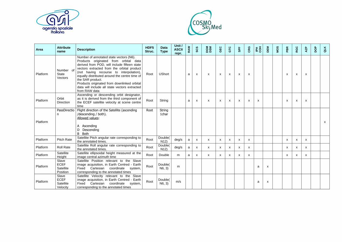
Area Attribute name Description HDF5
Struc. Data Type
Unit /ASCII repr. R
AW
SCS
DG
M
DSM
GEC
GTC
SPF
CR
G
IPH
C
OH
DEM
MO
S
PBR
RG
C
AZP
DO
P
QLK
Platform Number of State Vectors
Number of annotated state vectors (N6). Products originated from orbital data derived from POD, will include fifteen state vectors extracted from the orbital product (not having recourse to interpolation), equally distributed around the centre time of the SAR product. Products originated from downlinked orbital data will include all state vectors extracted from RAW data
Root UShort a x x x x x x x x x
Platform Orbit Direction
Ascending or descending orbit designator, as it is derived from the third component of the ECEF satellite velocity at scene centre time
Root String a x x x x x x x x x x
Platform
PassDirection
Flight direction of the Satellite (ascending /descending / both). Allowed values: A Ascending D Descending B Both
Root String 1char
x
Platform Pitch Rate Satellite Pitch angular rate corresponding to the annotated times. Root Double(
N12) deg/s a x x x x x x x x x
Platform Roll Rate Satellite Roll angular rate corresponding to the annotated times. Root Double(
N12) deg/s a x x x x x x x x x
Platform Satellite Height
Satellite ellipsoidal height measured at the image central azimuth time Root Double m a x x x x x x x x x
Platform
Slave ECEF Satellite Position
Satellite Position relevant to the Slave image acquisition, in Earth Centred - Earth Fixed Cartesian coordinate system, corresponding to the annotated times
Root Double(N6, 3) m a x
Platform
Slave ECEF Satellite Velocity
Satellite Velocity relevant to the Slave image acquisition, in Earth Centred - Earth Fixed Cartesian coordinate system, corresponding to the annotated times
Root Double(N6, 3) m/s a x
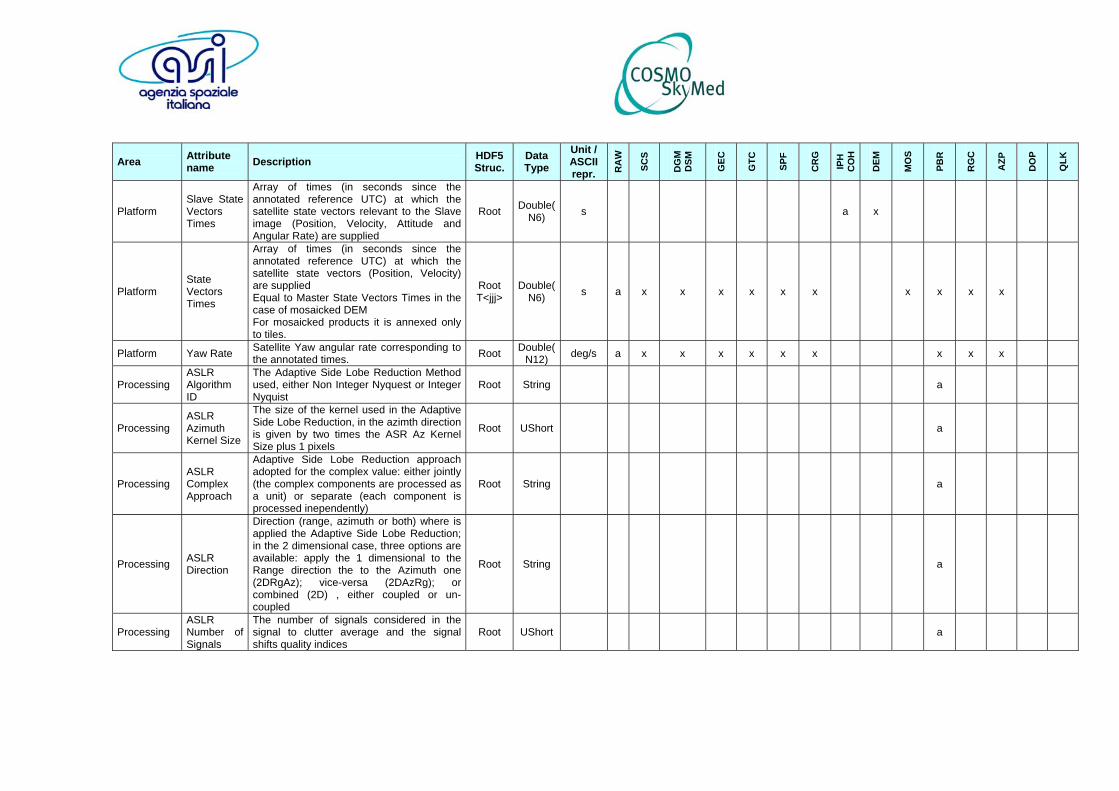
Area Attribute name Description HDF5
Struc. Data Type
Unit /ASCII repr. R
AW
SCS
DG
M
DSM
GEC
GTC
SPF
CR
G
IPH
C
OH
DEM
MO
S
PBR
RG
C
AZP
DO
P
QLK
Platform Slave State Vectors Times
Array of times (in seconds since the annotated reference UTC) at which the satellite state vectors relevant to the Slave image (Position, Velocity, Attitude and Angular Rate) are supplied
Root Double(N6) s a x
Platform State Vectors Times
Array of times (in seconds since the annotated reference UTC) at which the satellite state vectors (Position, Velocity) are supplied Equal to Master State Vectors Times in the case of mosaicked DEM For mosaicked products it is annexed only to tiles.
Root T<jjj>
Double(N6) s a x x x x x x x x x x
Platform Yaw Rate Satellite Yaw angular rate corresponding to the annotated times. Root Double(
N12) deg/s a x x x x x x x x x
Processing ASLR Algorithm ID
The Adaptive Side Lobe Reduction Method used, either Non Integer Nyquest or Integer Nyquist
Root String a
Processing ASLR Azimuth Kernel Size
The size of the kernel used in the Adaptive Side Lobe Reduction, in the azimth direction is given by two times the ASR Az Kernel Size plus 1 pixels
Root UShort a
Processing ASLR Complex Approach
Adaptive Side Lobe Reduction approach adopted for the complex value: either jointly (the complex components are processed as a unit) or separate (each component is processed inependently)
Root String a
Processing ASLR Direction
Direction (range, azimuth or both) where is applied the Adaptive Side Lobe Reduction; in the 2 dimensional case, three options are available: apply the 1 dimensional to the Range direction the to the Azimuth one (2DRgAz); vice-versa (2DAzRg); or combined (2D) , either coupled or un-coupled
Root String a
Processing ASLR Number of Signals
The number of signals considered in the signal to clutter average and the signal shifts quality indices
Root UShort a
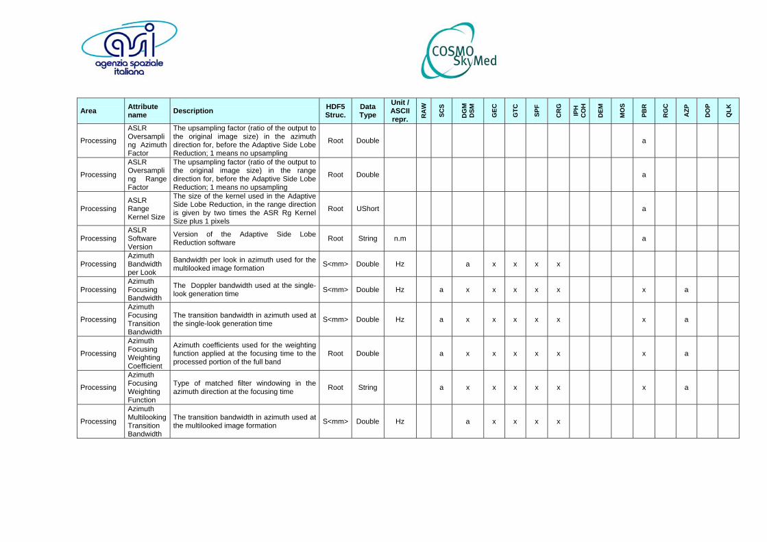
Area Attribute name Description HDF5
Struc. Data Type
Unit /ASCII repr. R
AW
SCS
DG
M
DSM
GEC
GTC
SPF
CR
G
IPH
C
OH
DEM
MO
S
PBR
RG
C
AZP
DO
P
QLK
Processing
ASLR Oversampling Azimuth Factor
The upsampling factor (ratio of the output to the original image size) in the azimuth direction for, before the Adaptive Side Lobe Reduction; 1 means no upsampling
Root Double a
Processing
ASLR Oversampling Range Factor
The upsampling factor (ratio of the output to the original image size) in the range direction for, before the Adaptive Side Lobe Reduction; 1 means no upsampling
Root Double a
Processing ASLR Range Kernel Size
The size of the kernel used in the Adaptive Side Lobe Reduction, in the range direction is given by two times the ASR Rg Kernel Size plus 1 pixels
Root UShort a
Processing ASLR Software Version
Version of the Adaptive Side Lobe Reduction software Root String n.m a
Processing Azimuth Bandwidth per Look
Bandwidth per look in azimuth used for the multilooked image formation S<mm> Double Hz a x x x x
Processing Azimuth Focusing Bandwidth
The Doppler bandwidth used at the single-look generation time S<mm> Double Hz a x x x x x x a
Processing
Azimuth Focusing Transition Bandwidth
The transition bandwidth in azimuth used at the single-look generation time S<mm> Double Hz a x x x x x x a
Processing
Azimuth Focusing Weighting Coefficient
Azimuth coefficients used for the weighting function applied at the focusing time to the processed portion of the full band
Root Double a x x x x x x a
Processing
Azimuth Focusing Weighting Function
Type of matched filter windowing in the azimuth direction at the focusing time Root String a x x x x x x a
Processing
Azimuth Multilooking Transition Bandwidth
The transition bandwidth in azimuth used at the multilooked image formation S<mm> Double Hz a x x x x

Area Attribute name Description HDF5
Struc. Data Type
Unit /ASCII repr. R
AW
SCS
DG
M
DSM
GEC
GTC
SPF
CR
G
IPH
C
OH
DEM
MO
S
PBR
RG
C
AZP
DO
P
QLK
Processing
Azimuth Multilooking Weighting Coefficient
Azimuth coefficients used for the weighting function applied at the multilooking time to each look
Root Double a x x x x
Processing
Azimuth Multilooking Weighting Function
Type of matched filter windowing in the azimuth direction at the multilooking time Root String a x x x x
Processing
Azimuth Processing Number of Looks
Number of processing azimuth looks Root UByte a m x x m x m x
Processing Baseline Calibration Flag
Flag indicating if the unwrapping has been applied (interferometric DEM) Root UByte a
Processing Beam Mosaicking Policy
Algorithm used for merging of overlapped beams (used only for ScanSAR mode, set to "N/A" otherwise)
Root String a x x x x x
Processing Column Spacing
Spacing among columns of the products. It is expressed in degrees in the case of GEODETIC projection, in meters otherwise.
SBI MBI Double m
deg a m m m x m m m m m
Processing Column Time Interval
Time spacing in the range direction between columns Set to invalid value in the case of ground projected products
SBI MBI Double s a x m m
Processing
CRG Coarse GCP Tolerance
Threshold for setting valid GCP after the coarse co-registration (both in master and slave images)
Root Double a
Processing
CRG Coarse Interpolation Factor
Coarse Registration Interpolation Factor in range and azimuth direction (both in master and slave images)
Root Double(2) a
Processing
CRG Coarse Window Size
Coarse Registration Window size in range and azimuth direction (both in master and slave images)
Root UShort(2) a
Processing CRG Coherence Tolerance
Threshold for setting valid GCP after the fine co-registration (both in master and slave images)
Root Double a

Area Attribute name Description HDF5
Struc. Data Type
Unit /ASCII repr. R
AW
SCS
DG
M
DSM
GEC
GTC
SPF
CR
G
IPH
C
OH
DEM
MO
S
PBR
RG
C
AZP
DO
P
QLK
Processing
CRG Coherence Window Size
Coherence Window size (both in master and slave images) Root Ushort(
2) a
Processing CRG Cubic Convolution Coefficient
Convolution Coefficient used in cubic interpolation performed on slave in the co-registration (both in master and slave images)
Root Double a
Processing CRG Fine Window Size
Fine Registration Window size in range and azimuth direction (both in master and slave images)
Root UShort(2) a
Processing CRG GCPs Selection Mode
Designator of the selection mode of GCPs for co-registration (both in master and slave images)
Root String a
Processing
CRG Interpolation Inverse Tolerance
The length of lookup tables used to speed up the sinc interpolation (both in master and slave images). High values give a good accuracy at the expense of an increased memory requirement. The accuracy that can be achieved is given by the reciprocal of this parameter, i.e. the default value (1000) gives an accuracy of 1/1000 of a pixel.
Root Double a
Processing CRG Interpolator ID
Designator of the type interpolation method performed on slave in the co-registration (both in master and slave images)
Root String a
Processing CRG Level ID
Designator of the type of performed co-registration (both in master and slave images)
Root String a
Processing CRG Number of GCPs
Number of GCPs in column (in the following N18) and row (in the following N19) directions
Root UInt(2) a
Processing CRG Overlap Type
Designator of the type of rectangular zone on which the co-registration is performed (both in master and slave images)
Root String a
Processing CRG Sinc Interpolator Length
Filter length used in sinc interpolation performed on slave in the co-registration: it is the filter size in row, col (both in master and slave images)
Root UShort(2) a
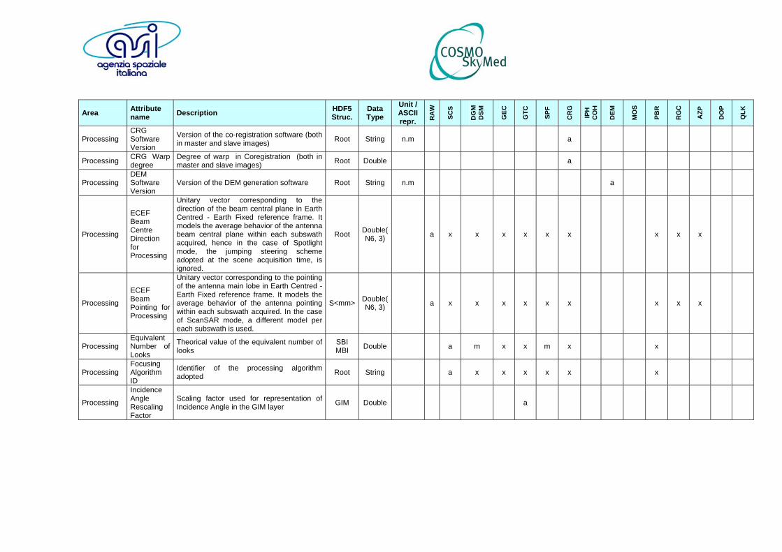
Area Attribute name Description HDF5
Struc. Data Type
Unit /ASCII repr. R
AW
SCS
DG
M
DSM
GEC
GTC
SPF
CR
G
IPH
C
OH
DEM
MO
S
PBR
RG
C
AZP
DO
P
QLK
Processing CRG Software Version
Version of the co-registration software (both in master and slave images) Root String n.m a
Processing CRG Warp degree
Degree of warp in Coregistration (both in master and slave images) Root Double a
Processing DEM Software Version
Version of the DEM generation software Root String n.m a
Processing
ECEF Beam Centre Direction for Processing
Unitary vector corresponding to the direction of the beam central plane in Earth Centred - Earth Fixed reference frame. It models the average behavior of the antenna beam central plane within each subswath acquired, hence in the case of Spotlight mode, the jumping steering scheme adopted at the scene acquisition time, is ignored.
Root Double(N6, 3) a x x x x x x x x x
Processing
ECEF Beam Pointing for Processing
Unitary vector corresponding to the pointing of the antenna main lobe in Earth Centred - Earth Fixed reference frame. It models the average behavior of the antenna pointing within each subswath acquired. In the case of ScanSAR mode, a different model per each subswath is used.
S<mm> Double(N6, 3) a x x x x x x x x x
Processing Equivalent Number of Looks
Theorical value of the equivalent number of looks
SBI MBI Double a m x x m x x
Processing Focusing Algorithm ID
Identifier of the processing algorithm adopted Root String a x x x x x x
Processing
Incidence Angle Rescaling Factor
Scaling factor used for representation of Incidence Angle in the GIM layer GIM Double a

Area Attribute name Description HDF5
Struc. Data Type
Unit /ASCII repr. R
AW
SCS
DG
M
DSM
GEC
GTC
SPF
CR
G
IPH
C
OH
DEM
MO
S
PBR
RG
C
AZP
DO
P
QLK
Processing Invalid Value
Value used to fill invalid pixels/lines. Are catalogued as invalid, the following categories of data: - compensated missing lines; - area of geocoded products outside the SAR sensed data limits. As far as portion of lines added by SWST readjustment, they are in any case filled by zero. In the case of complex dataset (hence represented by two samples per pixel), invalid pixels will be characterized by Invalid Value loaded in both of its channelsFor L0 product, invalid pixels are associated only to missing lines. Allowed values depend on the Product Type.
Root Float a a a a a a a a a a a a a a
Processing ITF Coherence Window
Coherence window estimation dimension (range, azimuth) Root UByte(
2) a
Processing
ITF Common Band Azimuth Filter Flag
Flag indicating if the azimuth filter has been applied Root UByte a
Processing
ITF Common Band Range Filter Flag
Flag indicating if the range filter has been applied Root UByte a
Processing
ITF Demodulation Phase Reference Surface
Designator of the surface used for the evaluation of the demodulation phase Root String a
Processing ITF Layover Filter Flag
Flag indicating if the layover filter has been applied Root UByte a
Processing ITF Software Version
Version of the interferometric software Root String n.m a
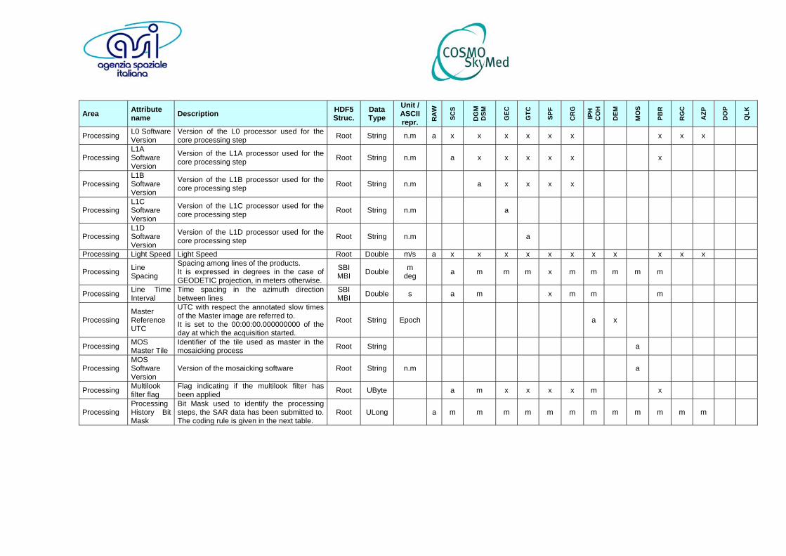
Area Attribute name Description HDF5
Struc. Data Type
Unit /ASCII repr. R
AW
SCS
DG
M
DSM
GEC
GTC
SPF
CR
G
IPH
C
OH
DEM
MO
S
PBR
RG
C
AZP
DO
P
QLK
Processing L0 Software Version
Version of the L0 processor used for the core processing step Root String n.m a x x x x x x x x x
Processing L1A Software Version
Version of the L1A processor used for the core processing step Root String n.m a x x x x x x
Processing L1B Software Version
Version of the L1B processor used for the core processing step Root String n.m a x x x x
Processing L1C Software Version
Version of the L1C processor used for the core processing step Root String n.m a
Processing L1D Software Version
Version of the L1D processor used for the core processing step Root String n.m a
Processing Light Speed Light Speed Root Double m/s a x x x x x x x x x x x
Processing Line Spacing
Spacing among lines of the products. It is expressed in degrees in the case of GEODETIC projection, in meters otherwise.
SBI MBI Double m
deg a m m m x m m m m m
Processing Line Time Interval
Time spacing in the azimuth direction between lines
SBI MBI Double s a m x m m m
Processing Master Reference UTC
UTC with respect the annotated slow times of the Master image are referred to. It is set to the 00:00:00.000000000 of the day at which the acquisition started.
Root String Epoch a x
Processing MOS Master Tile
Identifier of the tile used as master in the mosaicking process Root String a
Processing MOS Software Version
Version of the mosaicking software Root String n.m a
Processing Multilook filter flag
Flag indicating if the multilook filter has been applied Root UByte a m x x x x m x
Processing Processing History Bit Mask
Bit Mask used to identify the processing steps, the SAR data has been submitted to. The coding rule is given in the next table.
Root ULong a m m m m m m m m m m m m
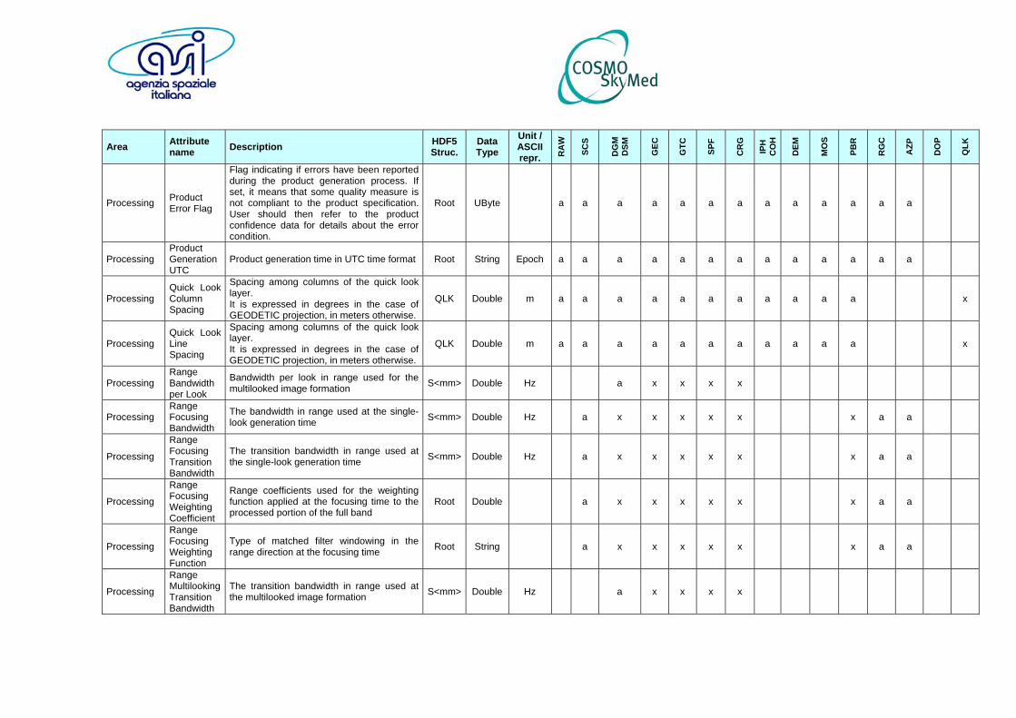
Area Attribute name Description HDF5
Struc. Data Type
Unit /ASCII repr. R
AW
SCS
DG
M
DSM
GEC
GTC
SPF
CR
G
IPH
C
OH
DEM
MO
S
PBR
RG
C
AZP
DO
P
QLK
Processing Product Error Flag
Flag indicating if errors have been reported during the product generation process. If set, it means that some quality measure is not compliant to the product specification. User should then refer to the product confidence data for details about the error condition.
Root UByte a a a a a a a a a a a a a
Processing Product Generation UTC
Product generation time in UTC time format Root String Epoch a a a a a a a a a a a a a
Processing Quick Look Column Spacing
Spacing among columns of the quick look layer. It is expressed in degrees in the case of GEODETIC projection, in meters otherwise.
QLK Double m a a a a a a a a a a a x
Processing Quick Look Line Spacing
Spacing among columns of the quick look layer. It is expressed in degrees in the case of GEODETIC projection, in meters otherwise.
QLK Double m a a a a a a a a a a a x
Processing Range Bandwidth per Look
Bandwidth per look in range used for the multilooked image formation S<mm> Double Hz a x x x x
Processing Range Focusing Bandwidth
The bandwidth in range used at the single-look generation time S<mm> Double Hz a x x x x x x a a
Processing
Range Focusing Transition Bandwidth
The transition bandwidth in range used at the single-look generation time S<mm> Double Hz a x x x x x x a a
Processing
Range Focusing Weighting Coefficient
Range coefficients used for the weighting function applied at the focusing time to the processed portion of the full band
Root Double a x x x x x x a a
Processing
Range Focusing Weighting Function
Type of matched filter windowing in the range direction at the focusing time Root String a x x x x x x a a
Processing
Range Multilooking Transition Bandwidth
The transition bandwidth in range used at the multilooked image formation S<mm> Double Hz a x x x x

Area Attribute name Description HDF5
Struc. Data Type
Unit /ASCII repr. R
AW
SCS
DG
M
DSM
GEC
GTC
SPF
CR
G
IPH
C
OH
DEM
MO
S
PBR
RG
C
AZP
DO
P
QLK
Processing
Range Multilooking Weighting Coefficient
Range coefficients used for the weighting function applied at the multilooking time to each look
Root Double a x x x x
Processing
Range Multilooking Weighting Function
Type of matched filter windowing in the range direction at the multilooking time Root String a x x x x
Processing
Range Processing Number of Looks
Number of nominal looks in the range direction Root UByte a m x x m x m x
Processing RAW Statistics Block Size
Size (in number of rows and number of columns) of the block where statistics on the RAW data are evaluated. In the following, N9 (resp. N10) will indicate the number of azimuth (resp. range) blocks (derived from the block size for statistics evaluation) in the burst over which statistics are evaluated. It is always assumed that: - first block for statistics evaluation is anchored to the first row/col of the burst - moving steps for other block determination is equal to the block size - block size is defined so that N9 <= 300 and N10 <= 3
S<mm> UInt(2) a x x x x x x x x x
Processing Reference UTC
UTC with respect the annotated slow times are referred to. It is set to the 00:00:00.000000000 of the day at which the acquisition started. For mosaicked products it is annexed only to tiles.
Root T<jjj> String Epoch a x x x x x x x x x x x
Processing Replica Reconstruction Method
Designator of method for reconstruction of chirp used for image processing. Set to invalid value in the Spotlight case.
Root String a x x x x x x
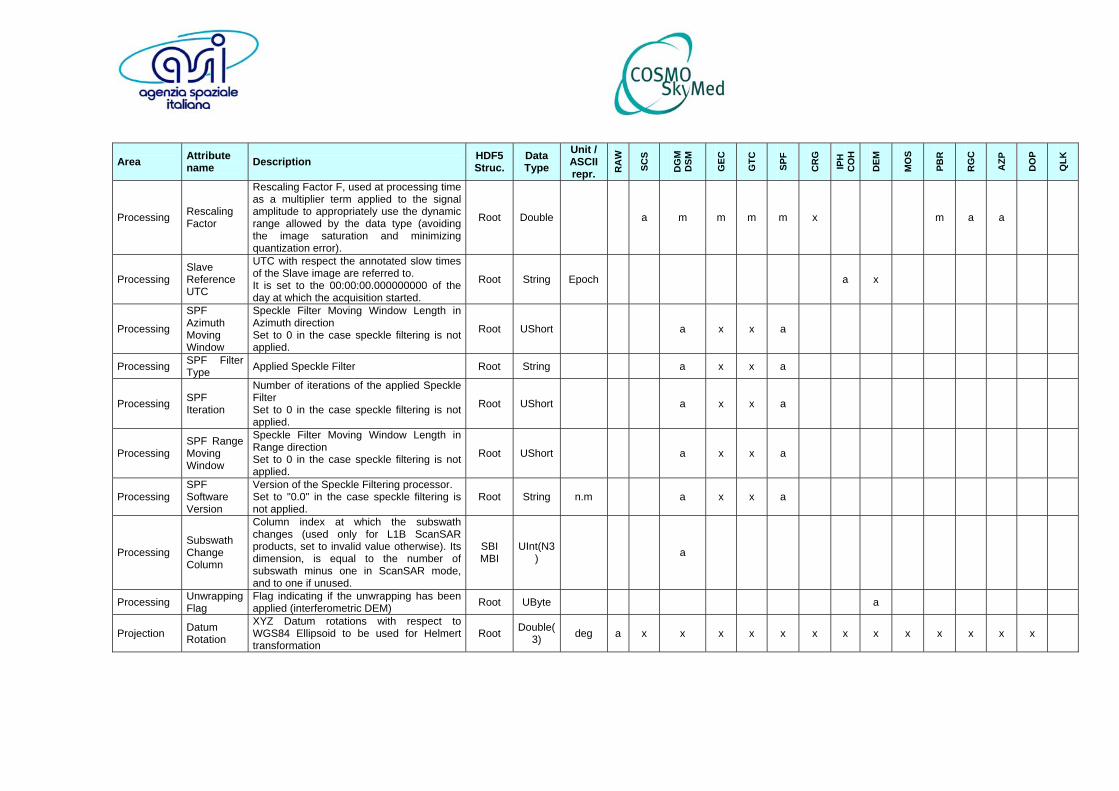
Area Attribute name Description HDF5
Struc. Data Type
Unit /ASCII repr. R
AW
SCS
DG
M
DSM
GEC
GTC
SPF
CR
G
IPH
C
OH
DEM
MO
S
PBR
RG
C
AZP
DO
P
QLK
Processing Rescaling Factor
Rescaling Factor F, used at processing time as a multiplier term applied to the signal amplitude to appropriately use the dynamic range allowed by the data type (avoiding the image saturation and minimizing quantization error).
Root Double a m m m m x m a a
Processing Slave Reference UTC
UTC with respect the annotated slow times of the Slave image are referred to. It is set to the 00:00:00.000000000 of the day at which the acquisition started.
Root String Epoch a x
Processing
SPF Azimuth Moving Window
Speckle Filter Moving Window Length in Azimuth direction Set to 0 in the case speckle filtering is not applied.
Root UShort a x x a
Processing SPF Filter Type Applied Speckle Filter Root String a x x a
Processing SPF Iteration
Number of iterations of the applied Speckle Filter Set to 0 in the case speckle filtering is not applied.
Root UShort a x x a
Processing SPF Range Moving Window
Speckle Filter Moving Window Length in Range direction Set to 0 in the case speckle filtering is not applied.
Root UShort a x x a
Processing SPF Software Version
Version of the Speckle Filtering processor. Set to "0.0" in the case speckle filtering is not applied.
Root String n.m a x x a
Processing Subswath Change Column
Column index at which the subswath changes (used only for L1B ScanSAR products, set to invalid value otherwise). Its dimension, is equal to the number of subswath minus one in ScanSAR mode, and to one if unused.
SBI MBI
UInt(N3) a
Processing Unwrapping Flag
Flag indicating if the unwrapping has been applied (interferometric DEM) Root UByte a
Projection Datum Rotation
XYZ Datum rotations with respect to WGS84 Ellipsoid to be used for Helmert transformation
Root Double(3) deg a x x x x x x x x x x x x x
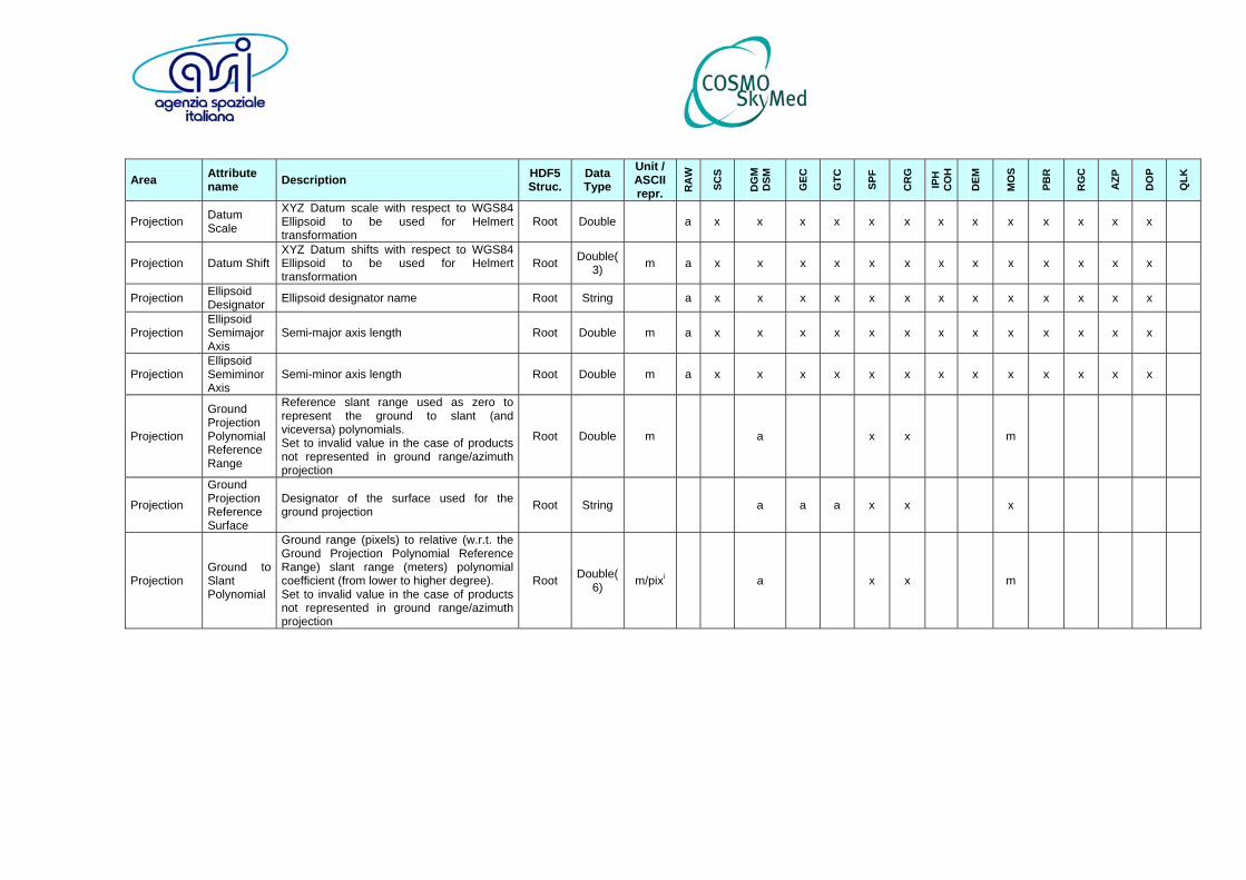
Area Attribute name Description HDF5
Struc. Data Type
Unit /ASCII repr. R
AW
SCS
DG
M
DSM
GEC
GTC
SPF
CR
G
IPH
C
OH
DEM
MO
S
PBR
RG
C
AZP
DO
P
QLK
Projection Datum Scale
XYZ Datum scale with respect to WGS84 Ellipsoid to be used for Helmert transformation
Root Double a x x x x x x x x x x x x x
Projection Datum Shift XYZ Datum shifts with respect to WGS84 Ellipsoid to be used for Helmert transformation
Root Double(3) m a x x x x x x x x x x x x x
Projection Ellipsoid Designator Ellipsoid designator name Root String a x x x x x x x x x x x x x
Projection Ellipsoid Semimajor Axis
Semi-major axis length Root Double m a x x x x x x x x x x x x x
Projection Ellipsoid Semiminor Axis
Semi-minor axis length Root Double m a x x x x x x x x x x x x x
Projection
Ground Projection Polynomial Reference Range
Reference slant range used as zero to represent the ground to slant (and viceversa) polynomials. Set to invalid value in the case of products not represented in ground range/azimuth projection
Root Double m a x x m
Projection
Ground Projection Reference Surface
Designator of the surface used for the ground projection Root String a a a x x x
Projection Ground to Slant Polynomial
Ground range (pixels) to relative (w.r.t. the Ground Projection Polynomial Reference Range) slant range (meters) polynomial coefficient (from lower to higher degree). Set to invalid value in the case of products not represented in ground range/azimuth projection
Root Double(6) m/pixi a x x m
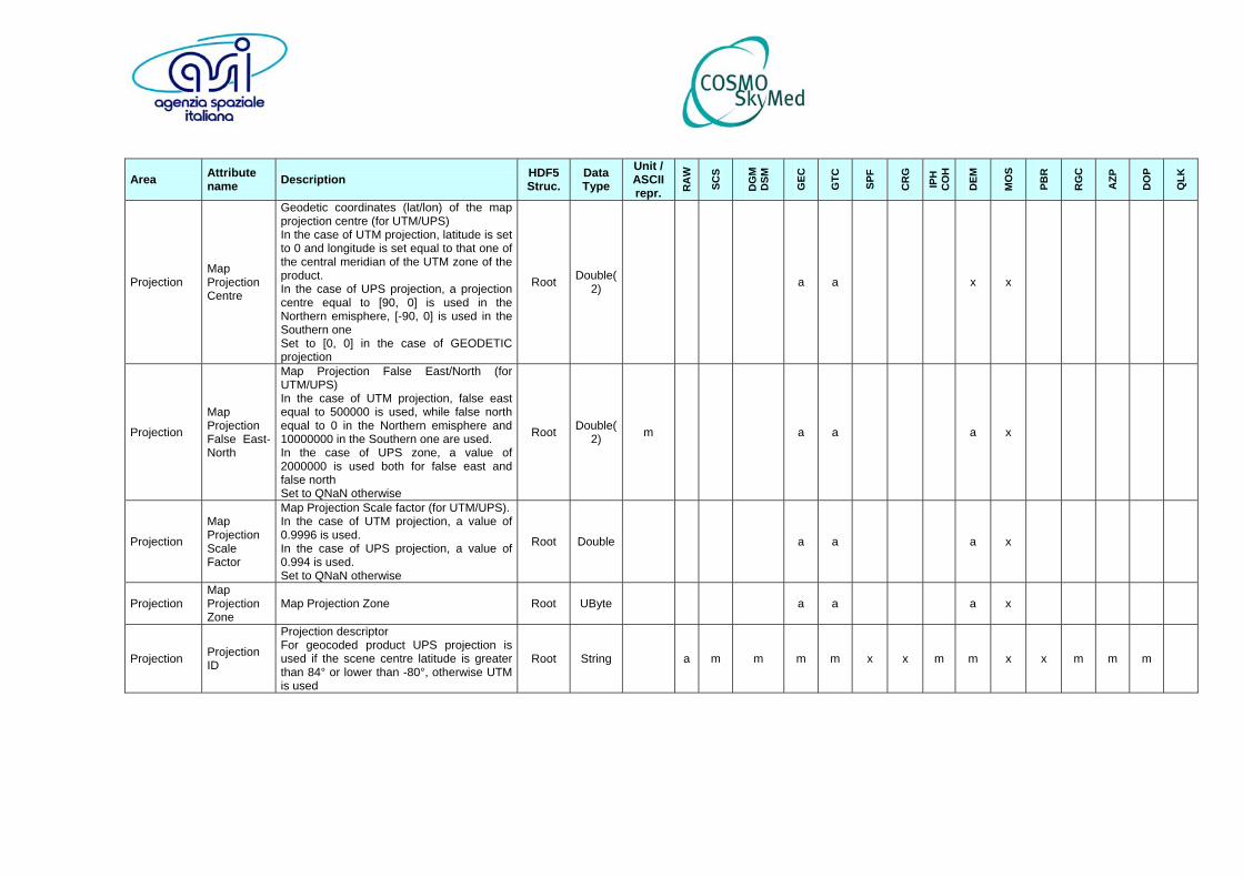
Area Attribute name Description HDF5
Struc. Data Type
Unit /ASCII repr. R
AW
SCS
DG
M
DSM
GEC
GTC
SPF
CR
G
IPH
C
OH
DEM
MO
S
PBR
RG
C
AZP
DO
P
QLK
Projection Map Projection Centre
Geodetic coordinates (lat/lon) of the map projection centre (for UTM/UPS) In the case of UTM projection, latitude is set to 0 and longitude is set equal to that one of the central meridian of the UTM zone of the product. In the case of UPS projection, a projection centre equal to [90, 0] is used in the Northern emisphere, [-90, 0] is used in the Southern one Set to [0, 0] in the case of GEODETIC projection
Root Double(2) a a x x
Projection
Map Projection False East-North
Map Projection False East/North (for UTM/UPS) In the case of UTM projection, false east equal to 500000 is used, while false north equal to 0 in the Northern emisphere and 10000000 in the Southern one are used. In the case of UPS zone, a value of 2000000 is used both for false east and false north Set to QNaN otherwise
Root Double(2) m a a a x
Projection
Map Projection Scale Factor
Map Projection Scale factor (for UTM/UPS).In the case of UTM projection, a value of 0.9996 is used. In the case of UPS projection, a value of 0.994 is used. Set to QNaN otherwise
Root Double a a a x
Projection Map Projection Zone
Map Projection Zone Root UByte a a a x
Projection Projection ID
Projection descriptor For geocoded product UPS projection is used if the scene centre latitude is greater than 84° or lower than -80°, otherwise UTM is used
Root String a m m m m x x m m x x m m m
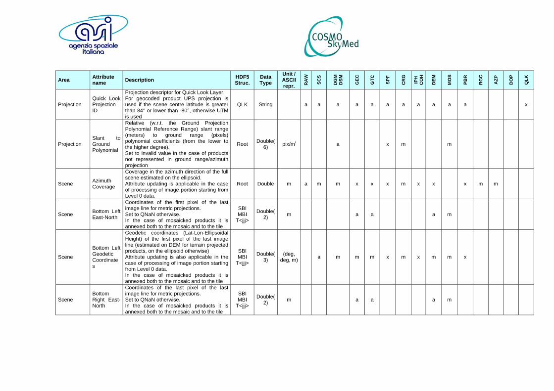
Area Attribute name Description HDF5
Struc. Data Type
Unit /ASCII repr. R
AW
SCS
DG
M
DSM
GEC
GTC
SPF
CR
G
IPH
C
OH
DEM
MO
S
PBR
RG
C
AZP
DO
P
QLK
Projection Quick Look Projection ID
Projection descriptor for Quick Look Layer For geocoded product UPS projection is used if the scene centre latitude is greater than 84° or lower than -80°, otherwise UTM is used
QLK String a a a a a a a a a a a x
Projection Slant to Ground Polynomial
Relative (w.r.t. the Ground Projection Polynomial Reference Range) slant range (meters) to ground range (pixels) polynomial coefficients (from the lower to the higher degree). Set to invalid value in the case of products not represented in ground range/azimuth projection
Root Double(6) pix/mi a x m m
Scene Azimuth Coverage
Coverage in the azimuth direction of the full scene estimated on the ellipsoid. Attribute updating is applicable in the case of processing of image portion starting from Level 0 data.
Root Double m a m m x x x m x x x m m
Scene Bottom Left East-North
Coordinates of the first pixel of the last image line for metric projections. Set to QNaN otherwise. In the case of mosaicked products it is annexed both to the mosaic and to the tile
SBI MBI
T<jjj>
Double(2) m a a a m
Scene
Bottom Left Geodetic Coordinates
Geodetic coordinates (Lat-Lon-Ellipsoidal Height) of the first pixel of the last image line (estimated on DEM for terrain projected products, on the ellipsoid otherwise) Attribute updating is also applicable in the case of processing of image portion starting from Level 0 data. In the case of mosaicked products it is annexed both to the mosaic and to the tile
SBI MBI
T<jjj>
Double(3)
(deg, deg, m) a m m m x m x m m x
Scene Bottom Right East-North
Coordinates of the last pixel of the last image line for metric projections. Set to QNaN otherwise. In the case of mosaicked products it is annexed both to the mosaic and to the tile
SBI MBI
T<jjj>
Double(2) m a a a m

Area Attribute name Description HDF5
Struc. Data Type
Unit /ASCII repr. R
AW
SCS
DG
M
DSM
GEC
GTC
SPF
CR
G
IPH
C
OH
DEM
MO
S
PBR
RG
C
AZP
DO
P
QLK
Scene
Bottom Right Geodetic Coordinates
Geodetic coordinates (Lat-Lon-Ellipsoidal Height) of the last pixel of the last image line (estimated on DEM for terrain projected products, on the ellipsoid otherwise) Attribute updating is also applicable in the case of processing of image portion starting from Level 0 data. In the case of mosaicked products it is annexed both to the mosaic and to the tile
SBI MBI
T<jjj>
Double(3)
(deg, deg, m) a m m m x m x m m x
Scene Centre Earth Radius
Earth radius at image centre Attribute updating is applicable in the case of processing of image portion starting from Level 0 data.
Root Double m a m m x x x x x x m x m m
Scene
Centre Geodetic Coordinates
Geodetic coordinates (lat-lon-height) of the central image point (estimated on DEM for terrain projected products, on the ellipsoid otherwise) of the swath. For RAW data it is estimated in acquisition geometry on the basis of the acquisition time of the central line discarding transients to be removed by range compression. Attribute updating is also applicable in the case of processing of image portion starting from Level 0 data.
S<mm> Double(3)
(deg, deg, m) a m m m m x m x x x m m
Scene
DeltaSideWardLookingAngle
Nominal look angle of the full observed swath (unsigned angle between nominal reference direction of the multi-beam and satellite nadir) expressed in millidegree
Root Uint 9digit
x
Scene
Estimated Bottom Left Geodetic Coordinates
Estimated geodetic coordinates (Lat-Lon-0) of the first pixel/last line of the correspendent focussed image
Root Double(3)
(deg, deg, m) a
Scene
Estimated Bottom Right Geodetic Coordinates
Estimated geodetic coordinates (Lat-Lon-0) of the last pixel/last line of the correspendent focussed image
Root Double(3)
(deg, deg, m) a
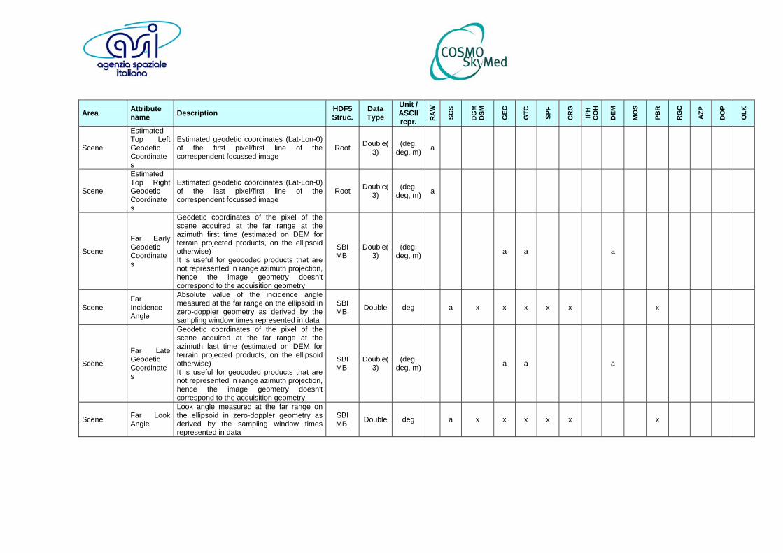
Area Attribute name Description HDF5
Struc. Data Type
Unit /ASCII repr. R
AW
SCS
DG
M
DSM
GEC
GTC
SPF
CR
G
IPH
C
OH
DEM
MO
S
PBR
RG
C
AZP
DO
P
QLK
Scene
Estimated Top Left Geodetic Coordinates
Estimated geodetic coordinates (Lat-Lon-0) of the first pixel/first line of the correspendent focussed image
Root Double(3)
(deg, deg, m) a
Scene
Estimated Top Right Geodetic Coordinates
Estimated geodetic coordinates (Lat-Lon-0) of the last pixel/first line of the correspendent focussed image
Root Double(3)
(deg, deg, m) a
Scene
Far Early Geodetic Coordinates
Geodetic coordinates of the pixel of the scene acquired at the far range at the azimuth first time (estimated on DEM for terrain projected products, on the ellipsoid otherwise) It is useful for geocoded products that are not represented in range azimuth projection, hence the image geometry doesn't correspond to the acquisition geometry
SBI MBI
Double(3)
(deg, deg, m) a a a
Scene Far Incidence Angle
Absolute value of the incidence angle measured at the far range on the ellipsoid in zero-doppler geometry as derived by the sampling window times represented in data
SBI MBI Double deg a x x x x x x
Scene
Far Late Geodetic Coordinates
Geodetic coordinates of the pixel of the scene acquired at the far range at the azimuth last time (estimated on DEM for terrain projected products, on the ellipsoid otherwise) It is useful for geocoded products that are not represented in range azimuth projection, hence the image geometry doesn't correspond to the acquisition geometry
SBI MBI
Double(3)
(deg, deg, m) a a a
Scene Far Look Angle
Look angle measured at the far range on the ellipsoid in zero-doppler geometry as derived by the sampling window times represented in data
SBI MBI Double deg a x x x x x x
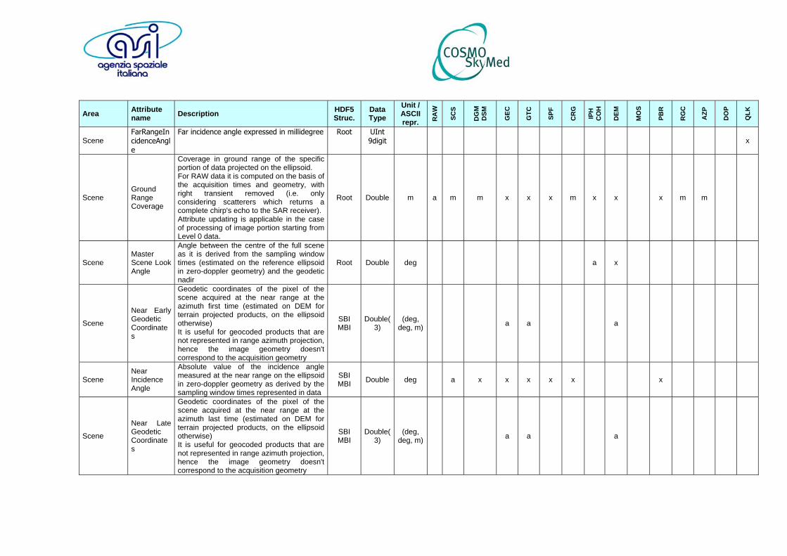
Area Attribute name Description HDF5
Struc. Data Type
Unit /ASCII repr. R
AW
SCS
DG
M
DSM
GEC
GTC
SPF
CR
G
IPH
C
OH
DEM
MO
S
PBR
RG
C
AZP
DO
P
QLK
Scene FarRangeIncidenceAngle
Far incidence angle expressed in millidegree Root UInt 9digit
x
Scene Ground Range Coverage
Coverage in ground range of the specific portion of data projected on the ellipsoid. For RAW data it is computed on the basis of the acquisition times and geometry, with right transient removed (i.e. only considering scatterers which returns a complete chirp's echo to the SAR receiver).Attribute updating is applicable in the case of processing of image portion starting from Level 0 data.
Root Double m a m m x x x m x x x m m
Scene Master Scene Look Angle
Angle between the centre of the full scene as it is derived from the sampling window times (estimated on the reference ellipsoid in zero-doppler geometry) and the geodetic nadir
Root Double deg a x
Scene
Near Early Geodetic Coordinates
Geodetic coordinates of the pixel of the scene acquired at the near range at the azimuth first time (estimated on DEM for terrain projected products, on the ellipsoid otherwise) It is useful for geocoded products that are not represented in range azimuth projection, hence the image geometry doesn't correspond to the acquisition geometry
SBI MBI
Double(3)
(deg, deg, m) a a a
Scene Near Incidence Angle
Absolute value of the incidence angle measured at the near range on the ellipsoid in zero-doppler geometry as derived by the sampling window times represented in data
SBI MBI Double deg a x x x x x x
Scene
Near Late Geodetic Coordinates
Geodetic coordinates of the pixel of the scene acquired at the near range at the azimuth last time (estimated on DEM for terrain projected products, on the ellipsoid otherwise) It is useful for geocoded products that are not represented in range azimuth projection, hence the image geometry doesn't correspond to the acquisition geometry
SBI MBI
Double(3)
(deg, deg, m) a a a

Area Attribute name Description HDF5
Struc. Data Type
Unit /ASCII repr. R
AW
SCS
DG
M
DSM
GEC
GTC
SPF
CR
G
IPH
C
OH
DEM
MO
S
PBR
RG
C
AZP
DO
P
QLK
Scene Near Look Angle
Look angle measured at the near range on the ellipsoid in zero-doppler geometry as derived by the sampling window times represented in data
SBI MBI Double deg a x x x x x x

Area Attribute name Description HDF5
Struc. Data Type
Unit /ASCII repr. R
AW
SCS
DG
M
DSM
GEC
GTC
SPF
CR
G
IPH
C
OH
DEM
MO
S
PBR
RG
C
AZP
DO
P
QLK
Scene NearRangeIncidenceAngle
Near incidence angle expressed in millidegree
Root UInt 9digit
x
Scene
Polygon List of vertex of the polygonal shape in term of Longitude and Latitude coordinates according to the following string format: [Point_1;Point_2;……. ;Point_x] where « Point_x » is defined as a couple Longitude:Latitude in the string format: FLOAT(010,5):FLOAT(010,6) with ranges, LONGITUDE: [-179.99999, 180.00000] ; LATITUDE: [-90.000000, 90.000000] . Vertex must be specified in a counter-clockwise direction. Closing point must not be included in the vertexes list Example: [-034.46557:067.684536;0156.37529:-63.760346;0156.16023:-63.741403;-034.21402:067.668000]
Root String
x

Area Attribute name Description HDF5
Struc. Data Type
Unit /ASCII repr. R
AW
SCS
DG
M
DSM
GEC
GTC
SPF
CR
G
IPH
C
OH
DEM
MO
S
PBR
RG
C
AZP
DO
P
QLK
Scene
Scene Centre Geodetic Coordinates
Geodetic coordinates (lat-lon-height) of the central image point (estimated on DEM for terrain projected products, on the ellipsoid otherwise) of the full scene For RAW data it is estimated in acquisition geometry on the basis of the acquisition time of the central line discarding transients (at the farthest subswath in the case of ScanSAR data) to be removed by range compression. Attribute updating is also applicable in the case of processing of image portion starting from Level 0 data.
Root Double(3)
(deg, deg, m) a m m x m x m x x m x m m
Scene Scene Orientation
Counter-clockwise measured angle between the local north at scene centre and the opposite of the azimuth oriented direction
Root Double deg a m m x x x m x x x m m
Scene
SceneCentre
Scene Centre Point Coordinates in the « Point_x » string format : FLOAT(6,2):FLOAT(6,2) as already detailed for Polygon attribute. Example: 60.96:1.96
Root String
x
Scene Slave Scene Look Angle
Angle between the centre of the full scene as it is derived from the sampling window times (estimated on the reference ellipsoid in zero-doppler geometry) and the geodetic nadir
Root Double deg a x
Scene
Terrain Elevation Standard Deviation
Standard deviation of the elevation of the observed scene Root Double m a
Scene Terrain Maximum Elevation
Maximum elevation of the observed scene Root Double m a
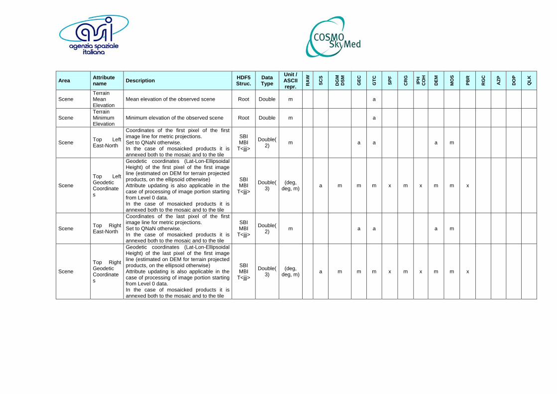
Area Attribute name Description HDF5
Struc. Data Type
Unit /ASCII repr. R
AW
SCS
DG
M
DSM
GEC
GTC
SPF
CR
G
IPH
C
OH
DEM
MO
S
PBR
RG
C
AZP
DO
P
QLK
Scene Terrain Mean Elevation
Mean elevation of the observed scene Root Double m a
Scene Terrain Minimum Elevation
Minimum elevation of the observed scene Root Double m a
Scene Top Left East-North
Coordinates of the first pixel of the first image line for metric projections. Set to QNaN otherwise. In the case of mosaicked products it is annexed both to the mosaic and to the tile
SBI MBI
T<jjj>
Double(2) m a a a m
Scene
Top Left Geodetic Coordinates
Geodetic coordinates (Lat-Lon-Ellipsoidal Height) of the first pixel of the first image line (estimated on DEM for terrain projected products, on the ellipsoid otherwise) Attribute updating is also applicable in the case of processing of image portion starting from Level 0 data. In the case of mosaicked products it is annexed both to the mosaic and to the tile
SBI MBI
T<jjj>
Double(3)
(deg, deg, m) a m m m x m x m m x
Scene Top Right East-North
Coordinates of the last pixel of the first image line for metric projections. Set to QNaN otherwise. In the case of mosaicked products it is annexed both to the mosaic and to the tile
SBI MBI
T<jjj>
Double(2) m a a a m
Scene
Top Right Geodetic Coordinates
Geodetic coordinates (Lat-Lon-Ellipsoidal Height) of the last pixel of the first image line (estimated on DEM for terrain projected products, on the ellipsoid otherwise) Attribute updating is also applicable in the case of processing of image portion starting from Level 0 data. In the case of mosaicked products it is annexed both to the mosaic and to the tile
SBI MBI
T<jjj>
Double(3)
(deg, deg, m) a m m m x m x m m x

Area Attribute name Description HDF5
Struc. Data Type
Unit /ASCII repr. R
AW
SCS
DG
M
DSM
GEC
GTC
SPF
CR
G
IPH
C
OH
DEM
MO
S
PBR
RG
C
AZP
DO
P
QLK
Sensor
SensingMethodActivePassiveType
Short Code for the active/passive type. Allowed values: A active sensor P passive sensor Set values: A active sensor
Root String 1char
x
Sensor
SensingMethodSensingType
Short Code for the sensing type. Allowed values: S earth surface sensing A atmospheric sounder L limb sounder atmospheric sensing V vertical altitude sensing Set values: S earth surface sensing
Root String 1char
x
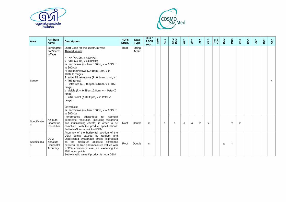
Area Attribute name Description HDF5
Struc. Data Type
Unit /ASCII repr. R
AW
SCS
DG
M
DSM
GEC
GTC
SPF
CR
G
IPH
C
OH
DEM
MO
S
PBR
RG
C
AZP
DO
P
QLK
Sensor
SensingMethodSpectrumType
Short Code for the spectrum type. Allowed values: h HF (λ>10m, v<50MHz) v VHF (λ>1m, v<300MHz) m microvawe (λ=1cm..100cm, v ~ 0.3GHz to 30GHz) M millimetrevawe (λ=1mm..1cm, v in 100GHz range) S sub-millimetrevawe (λ=0.1mm..1mm, v < THZ range) I infra-red (λ ~ 0.8μm..0.1mm, v > THZ range) V visible (λ ~ 0.39μm..0.8μm, v < PetaHZ range) U ultra-violet (λ<0.39μm, v in PetaHZ range) Set values: m microvawe (λ=1cm..100cm, v ~ 0.3GHz to 30GHz)
Root String 1char
x
Specification
Azimuth Geometric Resolution
Performance guaranteed for Azimuth geometric resolution (including weighting and multilooking effects) in order to be compliant with the product specifications. Set to NaN for mosaicked DEM.
Root Double m a a a a m x m m
Specification
DEM Absolute Horizontal Accuracy
Accuracy of the horizontal position of the DEM points caused by random and uncorrected systematic errors, expressed as the maximum absolute difference between the true and measured values with a 90% confidence level, i.e. excluding the 10% worst points. Set to invalid value if product is not a DEM
Root Double m a m
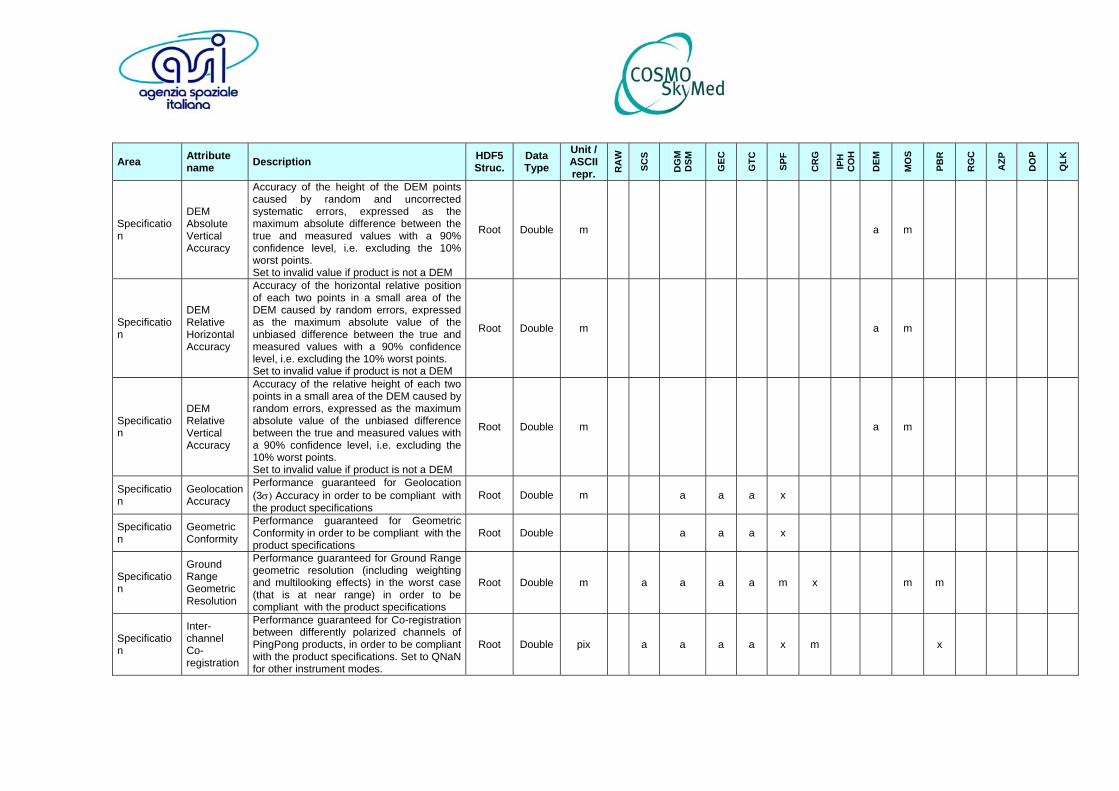
Area Attribute name Description HDF5
Struc. Data Type
Unit /ASCII repr. R
AW
SCS
DG
M
DSM
GEC
GTC
SPF
CR
G
IPH
C
OH
DEM
MO
S
PBR
RG
C
AZP
DO
P
QLK
Specification
DEM Absolute Vertical Accuracy
Accuracy of the height of the DEM points caused by random and uncorrected systematic errors, expressed as the maximum absolute difference between the true and measured values with a 90% confidence level, i.e. excluding the 10% worst points. Set to invalid value if product is not a DEM
Root Double m a m
Specification
DEM Relative Horizontal Accuracy
Accuracy of the horizontal relative position of each two points in a small area of the DEM caused by random errors, expressed as the maximum absolute value of the unbiased difference between the true and measured values with a 90% confidence level, i.e. excluding the 10% worst points. Set to invalid value if product is not a DEM
Root Double m a m
Specification
DEM Relative Vertical Accuracy
Accuracy of the relative height of each two points in a small area of the DEM caused by random errors, expressed as the maximum absolute value of the unbiased difference between the true and measured values with a 90% confidence level, i.e. excluding the 10% worst points. Set to invalid value if product is not a DEM
Root Double m a m
Specification
Geolocation Accuracy
Performance guaranteed for Geolocation (3σ) Accuracy in order to be compliant with the product specifications
Root Double m a a a x
Specification
Geometric Conformity
Performance guaranteed for Geometric Conformity in order to be compliant with the product specifications
Root Double a a a x
Specification
Ground Range Geometric Resolution
Performance guaranteed for Ground Range geometric resolution (including weighting and multilooking effects) in the worst case (that is at near range) in order to be compliant with the product specifications
Root Double m a a a a m x m m
Specification
Inter-channel Co-registration
Performance guaranteed for Co-registration between differently polarized channels of PingPong products, in order to be compliant with the product specifications. Set to QNaN for other instrument modes.
Root Double pix a a a a x m x
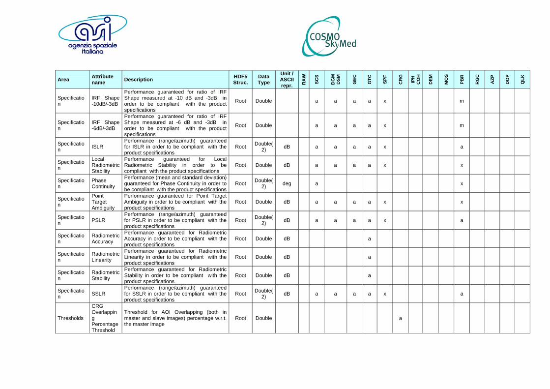
Area Attribute name Description HDF5
Struc. Data Type
Unit /ASCII repr. R
AW
SCS
DG
M
DSM
GEC
GTC
SPF
CR
G
IPH
C
OH
DEM
MO
S
PBR
RG
C
AZP
DO
P
QLK
Specification
IRF Shape -10dB/-3dB
Performance guaranteed for ratio of IRF Shape measured at -10 dB and -3dB in order to be compliant with the product specifications
Root Double a a a a x m
Specification
IRF Shape -6dB/-3dB
Performance guaranteed for ratio of IRF Shape measured at -6 dB and -3dB in order to be compliant with the product specifications
Root Double a a a a x m
Specification ISLR
Performance (range/azimuth) guaranteed for ISLR in order to be compliant with the product specifications
Root Double(2) dB a a a a x a
Specification
Local Radiometric Stability
Performance guaranteed for Local Radiometric Stability in order to be compliant with the product specifications
Root Double dB a a a a x x
Specification
Phase Continuity
Performance (mean and standard deviation) guaranteed for Phase Continuity in order to be compliant with the product specifications
Root Double(2) deg a x
Specification
Point Target Ambiguity
Performance guaranteed for Point Target Ambiguity in order to be compliant with the product specifications
Root Double dB a a a a x x
Specification PSLR
Performance (range/azimuth) guaranteed for PSLR in order to be compliant with the product specifications
Root Double(2) dB a a a a x a
Specification
Radiometric Accuracy
Performance guaranteed for Radiometric Accuracy in order to be compliant with the product specifications
Root Double dB a
Specification
Radiometric Linearity
Performance guaranteed for Radiometric Linearity in order to be compliant with the product specifications
Root Double dB a
Specification
Radiometric Stability
Performance guaranteed for Radiometric Stability in order to be compliant with the product specifications
Root Double dB a
Specification SSLR
Performance (range/azimuth) guaranteed for SSLR in order to be compliant with the product specifications
Root Double(2) dB a a a a x a
Thresholds
CRG Overlapping Percentage Threshold
Threshold for AOI Overlapping (both in master and slave images) percentage w.r.t. the master image
Root Double a

Area Attribute name Description HDF5
Struc. Data Type
Unit /ASCII repr. R
AW
SCS
DG
M
DSM
GEC
GTC
SPF
CR
G
IPH
C
OH
DEM
MO
S
PBR
RG
C
AZP
DO
P
QLK
Thresholds
Doppler Ambiguity Confidence Measure Threshold
Normalized confidence measure of doppler centroid ambiguity. A value of zero means poor confidence.
Root Double a x x x x x x x x x
Thresholds Doppler Ambiguity Threshold
Threshold for setting the Doppler Centroid ambiguity quality flag Root UShort a x x x x x x x x
Thresholds
Doppler Centroid Confidence Measure Threshold
Threshold for setting the Doppler Centroid confidence quality flag Root Double a x x x x x x x x x x
Thresholds
Doppler Centroid Estimation Accuracy Threshold
Threshold for setting the Doppler Centroid Accuracy quality flag Root Double Hz a x x x x x x x x x x
Thresholds
Doppler Rate Confidence Measure Threshold
Threshold for setting the Doppler Rate confidence quality flag Root Double a x x x x x x x x x
Thresholds
Doppler Rate Estimation Accuracy Threshold
Threshold for setting the Doppler Rate accuracy quality flag Root Double Hz/s a x x x x x x x x x
Thresholds
Image OverSaturated Percentage Threshold
Threshold for setting the OverSaturated Percentage quality flag Root Double a x x x x m x
Thresholds
Image UnderSaturated Percentage Threshold
Threshold for setting the UnderSaturated Percentage quality flag Root Double a x x x x m x
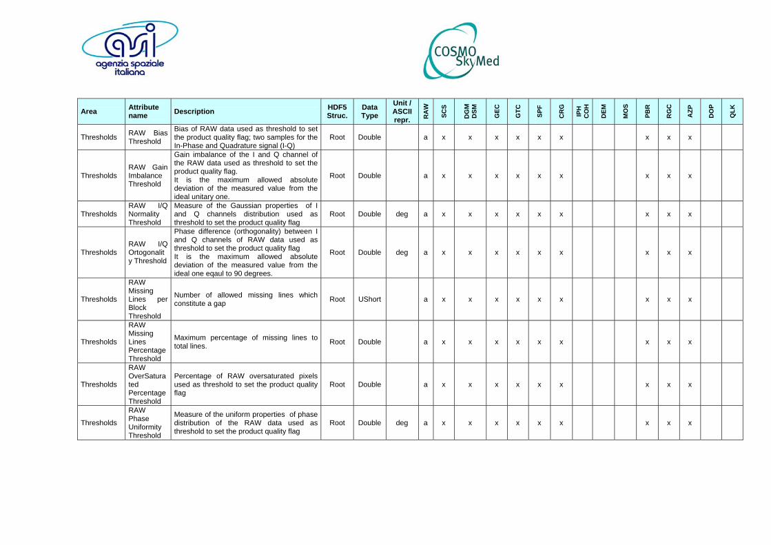
Area Attribute name Description HDF5
Struc. Data Type
Unit /ASCII repr. R
AW
SCS
DG
M
DSM
GEC
GTC
SPF
CR
G
IPH
C
OH
DEM
MO
S
PBR
RG
C
AZP
DO
P
QLK
Thresholds RAW Bias Threshold
Bias of RAW data used as threshold to set the product quality flag; two samples for the In-Phase and Quadrature signal (I-Q)
Root Double a x x x x x x x x x
Thresholds RAW Gain Imbalance Threshold
Gain imbalance of the I and Q channel of the RAW data used as threshold to set the product quality flag. It is the maximum allowed absolute deviation of the measured value from the ideal unitary one.
Root Double a x x x x x x x x x
Thresholds RAW I/Q Normality Threshold
Measure of the Gaussian properties of I and Q channels distribution used as threshold to set the product quality flag
Root Double deg a x x x x x x x x x
Thresholds RAW I/Q Ortogonality Threshold
Phase difference (orthogonality) between I and Q channels of RAW data used as threshold to set the product quality flag It is the maximum allowed absolute deviation of the measured value from the ideal one eqaul to 90 degrees.
Root Double deg a x x x x x x x x x
Thresholds
RAW Missing Lines per Block Threshold
Number of allowed missing lines which constitute a gap Root UShort a x x x x x x x x x
Thresholds
RAW Missing Lines Percentage Threshold
Maximum percentage of missing lines to total lines. Root Double a x x x x x x x x x
Thresholds
RAW OverSaturated Percentage Threshold
Percentage of RAW oversaturated pixels used as threshold to set the product quality flag
Root Double a x x x x x x x x x
Thresholds
RAW Phase Uniformity Threshold
Measure of the uniform properties of phase distribution of the RAW data used as threshold to set the product quality flag
Root Double deg a x x x x x x x x x

Area Attribute name Description HDF5
Struc. Data Type
Unit /ASCII repr. R
AW
SCS
DG
M
DSM
GEC
GTC
SPF
CR
G
IPH
C
OH
DEM
MO
S
PBR
RG
C
AZP
DO
P
QLK
Thresholds
RAW UnderSaturated Percentage Threshold
Percentage of RAW undersaturated pixels used as threshold to set the product quality flag
Root Double a x x x x x x x x x
Thresholds
Replica Geometric Resolution Threshold
Geometric resolution (meters in slant range) of the replica cross correlation function; it represents a threshold for setting the replica quality flag.
Root Double m a
Thresholds Replica ISLR Threshold
ISLR of the chirp cross correlation function; it represents a threshold for setting the chirp quality flag.
Root Double dB a
Thresholds Replica PSLR Threshold
PSLR of the chirp cross correlation function; it represents a threshold for setting the replica quality flag.
Root Double dB a
Thresholds
Replica Shape -10dB/-3dB Threshold
Aperture ratio of main lobe of reconstructed replica measured at -10 dB and -3dB; it represents a threshold for setting the replica quality flag.
Root Double dB a
Thresholds
Replica Shape -6dB/-3dB Threshold
Aperture ratio of main lobe of reconstructed replica measured at -10 dB and -3dB; it represents a threshold for setting the replica quality flag.
Root Double dB a
Thresholds Replica SSLR Threshold
SSLR of the chirp cross correlation function; it represents a threshold for setting the replica quality flag.
Root Double dB a

7 Acronyms and Glossary
7.1 Acronyms ASI Italian Space Agency
DEM Digital Elevation Model
DESS Digital Electronics SubSystem
ENL Equivalent Numbero of Looks
EO Earth Observation
GEC Geocoded Ellipsoid Corrected
GTC Geocoded Terrain Corrected
HDF Hierarchical Data Format
HK House Keeping
HW Hardware
I/F Interface
NE Noise Equivalent
PRI Precision Raw Image
SAR Synthetic Aperture Radar
SCS Single look, Complex, Slant Range products
SW Software
7.2 Glossary Acquisition Mode
One of the basic acquisition modes allowed by the SAR instrument
• Spotlight (Enhanced Spotlight, SMART) • ScanSAR (WideRegion, HugeRegion) • Stripmap (Himage, PingPong) DEM
Digital Elevation Model. Terrain height data given on a regular map grid.
DGM Product Synonymous with Level 1B Product GEC Product Synonymous with Level 1C Product GTC Product Synonymous with Level 1D Product Incidence angle
It is the angle measured between the slant range direction and the normal to the tangent plane to the Earth surface in the specified point on ground
Level 0 data L0 data (i.e. raw SAR telemetry) consists of time ordered echo data, obtained after decryption and before unpacking, and includes all UTC-dated auxiliary and ancillary data (e.g. orbit data, satellite’s position and velocity, geometric sensor model, payload status, calibration data) required to produce the other basic and intermediate products.
Level 0 Data File
One Image Segment File (ISF) formatted as a sequence of Source Packets or VCDU’s Data Zones (decrypted or not depending on decryption key availability).
The following standard processing levels are conceived for COSMO: Level 0 Product Level 0 product consists of time ordered echo data, obtained after decryption and decompression (i.e. conversion from BAQ encoded data to 8-bit uniformly quantised data) and after applying internal calibration and error compensation; this product shall include all the auxiliary data (e.g.: trajectography, accurately dated satellite’s co-ordinates and speed vector, geometric sensor model, payload status, calibration data,..) required to produce the other basic and intermediate products.
Level 1A Product Level 1A products (also indicated as Single-look Complex Slant (SCS)), consist of SAR focused data internally radiometric calibrated, in zero-doppler slant range-azimuth geometric projection, left at natural geometric spacing with associated ancillary data
Level 1B Product Level 1B products (also indicated as Detected Ground Multi-look (MDG)), consist of SAR focused data internally radiometric calibrated, de-speckled, amplitude detected, projected in zero-doppler ground
range-azimuth onto a reference ellipsoid or on a DEM, resampled at a regular spacing on ground with associated ancillary data.
Level 1C Product Level 1C class of products (also indicated as Geocoded Ellipsoid Corrected (GEC)) is constituted by input data projected onto a reference ellipsoid chosen among a predefined set, in a regular grid obtained from a cartographic reference system chosen among a predefined set with associated ancillary data
Level 1D Products Level 1D class of products (also indicated as Geocoded Terrain Corrected (GTC)) is constituted by input data projected onto a reference elevation surface in a regular grid obtained from a cartographic reference system chosen among a predefined set with associated ancillary data
Local incidence angle
The angle between the radar beam center and the normal to the local topography. The difference between the global incidence angle and the terrain slope.
Look angle
Of a SAR, the angle from the nadir at which the radar beam is pointed. Of a target, the angle between the SAR-nadir and SAR-target lines.
Raw Product
Synonymous of Level 0 Product
SAR Product
Generic term referring to the SAR data acquired in the different SAR modes and handled in the GS, at different level of processing (see also Level xxx Products).
The SAR products are catalogued in two classes:
- Standard products - Non-standard products
SCS Product
Synonymous of Level 1A Product