COSMO–SkyMed Synthetic Aperture Radar data to observe the

Article

COSMO–SkyMed Synthetic Aperture Radar data toobserve the Deepwater Horizon oil spill

Ferdinando Nunziata 1,∗ ID , Andrea Buono 1,∗ ID and Maurizio Migliaccio 1,∗ ID

1

2

3

4

5

6

7

8

9

10

11

1 Università degli Studi di Napoli Parthenope, Dipartimento di Ingegneria;nunziata,andrea.buono,[email protected]

* Correspondence: {nunziata,andrea.buono,migliaccio}@uniparthenope.it; Tel.: +39-081-547-6768

Abstract: Oil spills are adverse events that may be very harmful to ecosystems and food chain. In particular, large sea oil spills are very dramatic occurrence often affecting sea and coastal areas. Therefore the sustainability of oil rig infrastructures and oil transportation via oil tankers are linked to law enforcement based on proper monitoring techniques which are also fundamental to mitigate the impact of such pollution. Within this context, in this study a meaningful showcase is analyzed using remotely sensed measurements collected by by Synthetic Aperture Radar (SAR) satellites. The Deepwater Horizon (DWH) oil accident that occurred in the Gulf of Mexico in 2010 is here analyzed. It is one of the world’s largest accidental oil pollution event that affected a sea area larger than 10,000 km2. In this study we exploit SAR data collected by the Italian COSMO–SkyMed (CSK) X–band SAR constellation showing the key benefits of multi–polarization HH–VV SAR measurements in observing such a huge oil pollution event.

Keywords: Sea, remote sensing, oil pollution12

1. Introduction13

Oceans, seas and all the marine resources are essential to human well–being and social and14

economic development [1]. Oceans provide livelihoods, subsistence and benefits from fisheries,15

tourism and many other sectors, also helping in regulating the global ecosystem by absorbing heat16

and carbon dioxide from the atmosphere. However, oceans and coastal areas are severely susceptible17

to environmental degradation, overfishing, climate change, biodiversity loss and pollution [2]. In18

particular, pollutants significantly threat coastal regions and, since river basins, marine ecosystems19

and the atmosphere belong all together to the same hydrological systems, its effects are often found20

at far distance by the polluting source. According to the 2015 “Transboundary Waters Assessment21

Programme” global comparative assessment, the Gulf of Mexico is one of the five largest marine22

ecosystems mostly at risk of pollution and eutrophication. Hence, its preservation and sustainable23

management are key points to be achieved in the 2030 Agenda [3]. One of the goals mentioned in the24

sustainable development report of 2016 explicitly states “conserve and sustainably use the oceans, seas25

and marine resources for sustainable development” is of primary importance [4].26

Sea oil spills are the most noticeable forms of damage to the marine environment. Oil at sea comes27

from oil tanker or oil rig disasters, but also — and primarily — from diffuse sources, such as leaks28

during oil extraction, illegal tank–cleaning operations at sea, or discharges into the rivers which are29

then carried into the sea. Generally speaking, two classes of sea oil spill may occur, large oil spills and30

small oil spills. In the first case, we are dealing with macro oil spills; while in the second case we have31

micro oil spills. The size and duration of the spill, its chemical makeup and the marine environment32

are key factors to evaluate the short– and long–term ecological consequences of the spillage. While33

macro oil spills are well–known in general terms, the correct monitoring of the time evolving processes34

Preprints (www.preprints.org) | NOT PEER-REVIEWED | Posted: 30 May 2018 doi:10.20944/preprints201805.0442.v1

© 2018 by the author(s). Distributed under a Creative Commons CC BY license.

http://www.mdpi.com

https://orcid.org/0000-0000-000-000X

https://orcid.org/0000-0000-000-000X

https://orcid.org/0000-0000-000-000X

http://dx.doi.org/10.20944/preprints201805.0442.v1

http://creativecommons.org/licenses/by/4.0/

2 of 13

and the precise knowledge of the marine and coastal area affected is crucial. Micro oil spills are usually35

much more difficult to be monitored by patrol coast guard ships and airplanes, since they represent36

small–size events that may occurr in a large areas.37

Although proper monitoring is only the first part of a challenging scientific and operational processing38

chain it is important to be properly made [5]. In fact, although any macro oil spill has its unique39

characteristics, the logic processing chain is based on some key functional tools: monitoring, forecasting40

and vulnerability assessment. It must be noted that many uncertainties still remain especially in41

forecasting of an oil spill because of meteo–marine conditions and aging that make oil forecasting a42

complex process that cannot be standardized in a simple way. Hence, it is important to provide to43

the forecast modeler the best available information in terms of sea oil coverage and possibly sea oil44

type. Sea oil type has a direct impact on forecasting since when oil has a predominant component45

that is volatile the polluting contamination process is very different with respect to the case where46

heavy damping oil is predominant. Generally speaking, in order to mitigate the adverse effects of a47

sea oil spill, it is a paramount importance to monitor the event and to provide the best information to48

the operational people to support remediation actions and dispatch proper bulletin to fishermen and49

population [6].50

With reference to oil tanker security, especially after the Prestige accident in 2002, the use of double–hull51

tankers was meant as the primary source to limit the risk of accidents. Unfortunately, the recent Sanchi52

accident in 2018 demonstrated that this ship construction technology does not lead to zero risk. On the53

other side, oil rigs are more and more environmental risky as they move to deep and ultra–deep sea.54

The reference accident is the Deepwater Horizon (DWH) accident that occurred in 2010 in the Gulf of55

Mexico [7,8]. The oil spill industry sustainability is based on the increasing and increasing sea oil spill56

remediation capability and this is also based on the quality of the monitoring capability.57

In this framework, this study focuses on the benefit of satellite day–and–night high–resolution Synthetic58

Aperture Radar (SAR) monitoring during the DWH accident. In fact, among the various remote sensing59

tools, SAR could effectively address the user needs in case of such huge accidental polluting events in60

terms of:61

• area covered;62

63

• continuous and almost near real–time operability.64

SAR imaging characteristics provide several extra–benefits if compared to optical remote sensing, even65

though the latter is extensively used to retrieve rough estimations of oil thickness and chemical66

properties. However, optical measurements are severely affected by weather conditions and,67

furthermore, response efforts as the use of chemical dispersants, may alter oil slicks’ appearance68

by dispersing it in subsurfaces making the interpretation of optical data non–trivial at all [5,6].69

It is internationally recognized that oil spill response operational services obtain great benefits by70

utilizing airborne/satellite-based remote sensing for oil spill surveillance [9,10]. In fact, several71

countries and governmental agencies, e.g. the European Maritime Safety Agency, assist their72

operational services by providing remotely sensed measurements, especially by SAR imagery. The73

latter is an active, coherent, band–limited microwave high–resolution sensor that can make day– and74

night–time measurements almost independently of atmospheric conditions. Among the currently75

available SAR systems, the Italian COSMO–SkyMed (CSK) one is attractive from an operational point76

of view since it is a constellation of four X–band SARs, characterized by a very short revisit time, i. e.,77

≈ 12 hours, and it is able to operate in an incoherent dual–polarization mode (Ping Pong, PP, mode).78

The capability of CSK to support an operational monitoring of the oceans have been demonstrated in79

[11,12,13].80

SAR oil slick observation is physically possible because an oil slick damps the short gravity and81

capillary waves which are responsible for the backscattering to the SAR antenna and therefore a low82

backscattering return occurs. As a result, in the SAR image plane, a dark area is associated to an oil slick83

[14]. SAR oil spill detection is not an easy task, since SAR images are affected by multiplicative noise,84



3 of 13

known as speckle, which hampers the interpretability of such images. Furthermore, there are other85

physical phenomena, known as look–alikes, which can generate dark areas in SAR images not related to86

oil spills, such as biogenic films, low–wind areas, rain cells, internal waves and oceanic or atmospheric87

fronts [15]. Accordingly, tailored filtering techniques must be developed in order to minimize the88

number of false alarms. They are generally based on the use of single–polarization SAR data together89

with ancillary data [5,14,16]. In some cases, the distinction between oil slicks and biogenic films is based90

on optical data [5]. The importance of dual–polarization SAR measurements has been demonstrated in91

literature for oil slicks observation purposes [17,18,19]. Nevertheless, although it has been physically92

demonstrated by theoretical modelling and experiments that polarimetric SAR measurements are the93

most adequate source to monitor oil slicks at sea [10,20], it is important to analyze, especially in the94

occurrence of large oil spill accidents, how all the available SAR measurements can be exploited at95

best.96

In this study a multi–polarization analysis of the capabilities of dual–polarization PP mode X–band97

CSK SAR data is first undertaken focusing on the DWH oil spill. The latter was extensively monitored98

by means of L–, C– and X–band SAR systems but, to the best of our knowledge, no study exploited99

the incoherent CSK PP mode to consider such a huge oil spill event [21,22,23,24]. Oil spill detection100

and estimation of the polluted area is undertaken using a textural–based image processing approach,101

while a multi–polarization analysis is undertaken in order to characterize the contrast, i. e., the ratio102

between the Normalized Radar Cross Section (NRCS) relevant to the slick–free and oil–covered sea103

surface, both in the HH and VV channels.104

Experiments, accomplished over X–band HH–VV PP mode Single–look Complex Slant (SCS) Level 1A105

CSK SAR data collected in the Gulf of Mexico over the polluted area, demonstrate the importance of106

the Italian constellation of CSK SAR satellites for an effective observation of sea oil slicks.107

2. The Deepwater Horizon accidental oil spill: a case study108

On 20 April 2010, a fire broke out on the Transocean DWH oil rig under lease to British Petroleum109

(BP), with 126 people on board (see Figure 1 (a)). After a large explosion, all but 11 of the crew managed110

to escape as the rig was overwhelmed by fire. On 22 April 2010, the rig sank. Safeguards set in place to111

automatically cap the oil well in case of catastrophe did not work as expected. According to a first112

conservative Minerals Management Service formula, BP estimated at worst a spill of 162,000 barrels113

per day and a standard technology recovery capacity of about 500,000 barrels per day. Only after 12114

weeks did BP succeed in placing a tight cap on the well. A first estimate of about 5 million barrels115

[25,26] already makes this accident the world’s largest accidental oil spill and, by far, the worst oil116

disaster in United States history. It is surpassed only by the intentional 1991 Gulf War spill in Kuwait.117

Oil spilled from the DWH wellhead was a Mississippi Canyon Block 252 (MS252) South Louisiana118

sweet, i. e., low in sulfur concentration, crude oil and, as far as for all the crude oils, it consists of119

thousands of chemical compounds [25,26]. The vast and persistent DWH spill challenged response120

capabilities which called for quantitative oil assessment at synoptic and operational scales. Although121

nowadays oil spill response still mainly relies on experienced observers, few trained observers and122

confounding factors, including weather, oil emulsification and scene illumination geometry presented123

very non-trivial challenges [7,27]. Moreover, the DWH spill was characterised by some key peculiarities124

that made its observation very challenging:125

• the spill originated from a water–depth of 1500 m. This has confounded many problems on126

understanding the behaviour of the oil [28,29]. In general, oil at sea is influenced by a number of127

advective processes, e.g. wind and wave advection, spreading, etc., and weathering. The latter is128

a non–advective process that alters the oil’s chemical and physical properties. In addition to the129

conventional weathering process on the surface, the DWH oil was subjected to weathering as it130

ascended from the well. In fact, DWH oil appeared to be incorporating water as it emerged on131

the surface [28,29];132

133



4 of 13

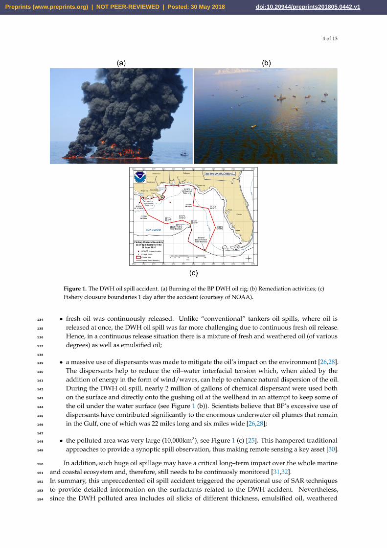
Figure 1. The DWH oil spill accident. (a) Burning of the BP DWH oil rig; (b) Remediation activities; (c)Fishery clousure boundaries 1 day after the accident (courtesy of NOAA).

• fresh oil was continuously released. Unlike “conventional” tankers oil spills, where oil is134

released at once, the DWH oil spill was far more challenging due to continuous fresh oil release.135

Hence, in a continuous release situation there is a mixture of fresh and weathered oil (of various136

degrees) as well as emulsified oil;137

138

• a massive use of dispersants was made to mitigate the oil’s impact on the environment [26,28].139

The dispersants help to reduce the oil–water interfacial tension which, when aided by the140

addition of energy in the form of wind/waves, can help to enhance natural dispersion of the oil.141

During the DWH oil spill, nearly 2 million of gallons of chemical dispersant were used both142

on the surface and directly onto the gushing oil at the wellhead in an attempt to keep some of143

the oil under the water surface (see Figure 1 (b)). Scientists believe that BP’s excessive use of144

dispersants have contributed significantly to the enormous underwater oil plumes that remain145

in the Gulf, one of which was 22 miles long and six miles wide [26,28];146

147

• the polluted area was very large (10,000km2), see Figure 1 (c) [25]. This hampered traditional148

approaches to provide a synoptic spill observation, thus making remote sensing a key asset [30].149

In addition, such huge oil spillage may have a critical long–term impact over the whole marine150

and coastal ecosystem and, therefore, still needs to be continuosly monitored [31,32].151

In summary, this unprecedented oil spill accident triggered the operational use of SAR techniques152

to provide detailed information on the surfactants related to the DWH accident. Nevertheless,153

since the DWH polluted area includes oil slicks of different thickness, emulsified oil, weathered154



5 of 13

oil, oil/dispersant mixture, fresh oil, etc., the surface slick is very heterogeneous, including different155

kind of surfactants. This implies that a synergistic use of different SAR operating modes is needed. In156

fact, large–swath imaging modes, i. e., ScanSAR, allow obtaining information on the extent of the oil157

spill, while narrower swath polarimetric modes, i. e., PP, allow extracting deeper information on the158

oil’s backscattering.159

3. Experiments and discussion160

In this section experiments undertaken on multi–polarization SCS CSK SAR data collected over161

the Gulf of Mexico area affected by the DWH accident are presented and discussed to demonstrate162

their potential in detecting the oil spill and to analyze the slick–free and oil–covered sea surface163

backscattering under different polarizations.164

The CSK SAR data set consists of two SAR scenes collected in right–looking ascending orbit over the165

DWH accidental oil spill site in the very next days after the accident, see Figure 2. The first SAR scene166

(product ID: 2006020) was acquired from the satellite “3” of the constellation on April 23, 2010, i. e.,167

only 3 days after the oil spillage just after the BP oil rig sank, in dual–polarization HH–VV PingPong168

mode under an incidence angle of 40◦ at mid–range. The SAR image consists of a 4123 × 18042 pixels169

covering an area of 30 km × 30 km with about 5 m × 2 m (range × azimuth) spatial resolution.170

A key parameter when observing sea oil slicks by SAR imagery is wind speed. In fact, it is unanimously171

recognized that SAR oil slick observation is possible when moderate wind conditions, i. e., wind172

speed ranges from about 2 m/s up to approximately 13 m/s [9,33]. When higher wind conditions173

apply, mixing phenomena dominate making the detectability of oil with respect to the surrounding174

sea impossible. At lower wind speeds, sea surface backscattering is comparable to the scattering from175

the oil slick; hence, even in this case oil–sea separability is not possible. Typically wind information is176

provided by ancillary remotely sensed data, e. g., scatterometer/radiometer or buoy measurements.177

Unfortunately, very often the information coming from other remotely sensed sources is not co–located178

in time and/or space with the available SAR data set. In addition, buoys co–located to the accident179

point are not always available.180

Hence, in this study a different approach is proposed that consists of providing a wind map by181

processing the SAR image. Different methods are available in literature that are mainly based on182

the exploitation of a scatterometer–like Geophsyical Model Function (GMF) to extract wind speed183

information once a priori wind direction information is available [34,35,36]. In this study, a spectral184

approach is considered that does not require any a priori wind direction information to provide the185

wind speed map. This approach is based on the inherent SAR peculiarities, i. e., the low–pass filtering186

in the azimuth direction due to the orbital motion of the sea surface waves that distorts the Doppler187

history of the backscattered waves [37,38]. The wind map, generated using the azimuth cut–off method,188

is shown in Figure 3 where the oil–covered area is masked out. It can be noted that low–to–moderate189

wind regime applies that is characterized by a mean wind speed of 7 m/s at the SAR acquisition time.190

Hence, SAR sea oil slick detection can be effectively undertaken.191

3.1. Oil spill detection192

In this subsection a texture–based oil spill detection procedure is undertaken to assess the potential193

of CSK SAR data to detect the DWH oil spill and to estimate its surface extent.194

In order to extract suitable intensity–based features that allow obtaining the oil spill detection binary195

mask, a textural–based feature extraction algorithm is adopted using the Gray–Level Co–occurrence196

Matrix (GLCM). The latter is one of the most popular statistical method to extract second–order texture197

features from remotely sensed images. The technique has been already successfully exploited in a198

broad range of SAR applications, e. g., ice–cover classification [39] and oil detection [40]. Basically,199

GLCM is a mathematical formalism that takes into account how often different pixel intensity value200

combinations occur in a remotely sensed image within given distances and directions. Among the basic201

GLCM parameters that can be extracted from a SAR image, which include mean, variance, correlation,202



6 of 13

Figure 2. Multi–polarization CSK SAR imagery relevant to the acquisition collected on 23 April 2010.(a) HH– and (b) VV–polarized NRCS graytone images (dB scale).

Figure 3. Azimuth cut–off based wind speed map derived from the CSK SAR scene collected on 23April 2010.



7 of 13

Figure 4. ASM–based oil detection maps relevant to the CSK SAR scene collected on 23 April 2010. (a)HH and (b) VV channel.

entropy, homogeneity, energy, contrast, dissimilarity, etc., the Angular Second Moment (ASM) was203

found to be the most effective in separating the oiled area from the surrounding sea. ASM is defined204

as ∑Ni,j=0[I(i, j)]2, where P is the original intensity SAR image and N is the number of gray levels [41].205

ASM can be seen as a measure of homogeneity of the intensity SAR image. Since the oiled area is206

expected to be more homogeneous than the sea surface, i. e., few gray levels are present, it will be207

characterized by few and relatively high intensity values I(i, j) that result in ASM values larger than208

the ones characterizing sea surface. In this study, quantization in N = 32 gray levels and a 9 × 9 sliding209

window are used to estimate ASM.210

Oil spill detection results are shown in Figure 4, where the binary masks obtained thresholding the211

ASM images are obtained from HH and VV channel (see Figure 4 (a) and (b), respectively). A threshold212

ASM = 1 is empirically set. Post–processing techniques, i. e., a morphological filter, is then applied to213

derive the oil detection maps of Figure 4. It can be noted that the oil detection mask obtained from214

the VV NRCS clearly separates the polluted area, that calls for ASM values larger than 1 due to its215

homogeneity, from the surrounding sea, that represents a more heterogeneous scenarios resulting in216

a lower ASM values (see Figure 4 (b)). Please note also that the few isolated black spots related to217

metallic targets at sea involved in cleaning–up operations (see bright spots in Figure 2) are visible in the218

oil spill detection map. This is likely due to the fact that they behave as very homogeneous scatterers.219

The oil spill can be detected even from the HH NRCS, although a very slightly larger number of false220

alarms and missed oil pixels within the slick are observed, see Figure 4 (a).221

Hence, according to the detection map of Figure 4 (b), the extent of the DWH oil spill can be estimated222

to be approximately 100 km2 at the SAR acquisition time, i. e., 3 days after the accident.223

3.2. Multi–polarization analysis224

In this subsection a multi–polarization analysis is undertaken to discuss the sensitivity of HH–225

and VV–polarized NRCS, σ0HH and σ0

VV , respectively, to slick–free and oil–covered backscattering.226

The two intensity channels are jointly used to generate the Pauli false–color RGB images of Figure 5227

where the following color–coding is adopted: R (σ0VV); G (σ0

HH) and B (σ0HH - σ0

VV). It can be noted228

that the joint use of VV and HH channels provides further information that can be exploited to gain229

a better understanding of the scattering processes. The backscattering from metallic targets (mostly230

due to ships and oil/gas drilling platforms), see brighter spots in Figure 2, is significantly larger than231

the sea one at both HH and VV polarizations. Sea surface backscattering results in VV–polarized232

backscattering larger tha the oil–covered area, as expected from the Bragg/tilted–Bragg theory. The233



8 of 13

Table 1. Multi–polarization analysis results.

Transect ROI σ0VV (dB) σ0

HH (dB) ∆VV (dB) ∆HH (dB)

Azimuth Sea -24.13 -27.34 12.43 10.53

DirectionOil -36.59 -37.86

Range Sea -22.62 -25.85 14.40 12.11

DirectionOil -37.00 -37.96

Table 2. Statistical oil–sea separability.

Parameter HH VVOil–sea JM 0.8232 1.0763

Overlapped area (%) 50 40

smallest difference between VV– and HH–polarized backscattering is achieved within the oil–covered234

areas. From a physical viewpoint, this can be explained considering that oil layer reduces significantly235

Bragg scattering waves leading to a noise–like backscattering which results in practically no difference236

between HH and VV channels.237

To provide a quantitative analysis of VV and HH backscattering over slick–free and oil–covered sea238

surface, σ0VV and σ0

HH values related to the azimuth– and range–oriented transects, see white dashed239

lines in Figure 2, are depicted in Figure 6. Values related to the along–range transect are depicted in240

Figure 6 (a), where one can not that: over slick–free sea surface σ0VV > σ0

HH (the difference is about 3241

dB) since Bragg scattering applies; within the oiled area, the backscattering is significantly lower than242

the sea one and there is negligible difference between HH and VV channels (the difference is less than243

1 dB). Same comments apply for the azimuth–oriented transect, see Figure 6 (b). The mean values244

related to slick–free and oil–covered σ0 values evaluated along with this transect are listed in Table 1245

where the contrast ∆, i. e., the slick–free to oil–covered σ0 ratio, is also listed for both the channels. As246

expected, the VV–polarized contrast is larger than the HH one (of about 2 dB) due to the larger sea247

surface backscattering in VV channel.248

To further discuss sea–oil backscattering separability, two equal–size Region of Interest (ROIs) kept249

within the oiled area and the slick–free sea surface are considered and the empirical probability density250

function (pdf) related to σ0 values are shown for both the VV and HH channels, see Figure 7. It can251

be noted that there is a good oil–sea separability at both HH and VV polarization according to the252

Jeffries–Matusita (JM) distance, see Table 2. The JM distance is defined as JM = 2(1-e−B), where B =253

-ln(∑x∈X

√(p(x)q(x)

)is the Bhattacharyya distance between the distribution pixel x belonging to254

slick–free (p) and oil–covered (q) ROIs [42]. In fact, the minimum JM value, i. e., 0, means that the two255

distribution are completely overlapped while the maximum JM value, i. e., 2, means totally separated256

distributions.257

Results listed in Table 2 clearly show that the largest oil–sea separation is provided by VV channel258

(JM = 1.0763) with a 40% overlapping between oil and sea pdfs. However, even when the HH channel259

performs fine in oil–sea separation (JM = 0.8232) with an overlapping equal to 50%. It can be also260

observed that the largest separation is provided by the combination of σ0HH evaluated over oil and σ0

VV261

evaluated over slick–free sea surface.262



9 of 13

Figure 5. False–color RGB image relevant to the CSK SAR scene collected on 23 April 2010, where thefollowing color–coding is adopted: R ≡ σ0

VV , G ≡ σ0HH and B ≡ σ0

HH – σ0VV .

Figure 6. HH– and VV–polarized NRCS values (in dB) evaluated along with the range– (a) andazimuth–oriented (b) transects shown in Figure 2.



10 of 13

Figure 7. Empirical pdfs related to σ0 values evaluated over the slick–free and oil–covered sea surfaceROIs for both the VV and HH channels.

4. Conclusions263

In this study, the capability of multi–polarization CSK SAR data, gathered in dual–polarization PP264

mode over the Gulf of Mexico, to observe the DWH accidental oil spill is investigated. Experimental265

results showed that:266

• CSK SAR data can be successfully employed to support local authorities in remediation and267

mitigation activity plans and the sustainability of coastal areas in case of offshore environmental268

disasters;269

270

• The observation of the DWH oil spill can take full benefits of the fine–resolution, dense revisit271

time and wide area coverage offered by the CSK satellites constellation;272

273

• The net extent of the DWH oil spill within 3 days of first oil release was about 100 km2;274

275

• The mean σ0VV sea–oil contrast is always larger than the σ0

HH one;276

277

• The largest separation is provided by the combination of σ0HH evaluated over oil and σ0

VV278

evaluated over slick–free sea surface.279

Acknowledgments: This study is partly funded by the Università degli Studi di Napoli Parthenope, project ID280

DING202. We thank the Italian Space Agency (ASI) that has provided the CSK SAR data under the project ID281

1221. Authors would also acknowledge ASI and E–Geos for useful discussions.282

Author Contributions: Ferdinando Nunziata and Maurizio Migliaccio conceived and designed the experiments;283

Andrea Buono and Ferdinando Nunziata performed the experiments and analyzed the data; Ferdinando Nunziata,284

Andrea Buono and Maurizio Migliaccio wrote the paper.285

Conflicts of Interest: The authors declare no conflict of interest. The founding sponsors had no role in the design286

of the study; in the collection, analyses, or interpretation of data; in the writing of the manuscript, and in the287

decision to publish the results.288

Abbreviations289

The following abbreviations are used in this manuscript:290

291



11 of 13

SAR Synthetic Aperture RadarDWH DeepWater HorizonCSK COSMO–SkyMedH HorizontalV VerticalPP PingPongNRCS Normalized Radar Cross–SectionSCS Single–look Complex SlantBP British PetroleumNOAA National Oceanic and Atmospheric AgencyGMF Geophsyical Model FunctiondB DecibelGLCM Gray–Level Co–occurrence MatrixASM Angular Second MomentRGB Red Green BlueROI Region Of Interestpdf Probability Density FunctionJM Jeffries–MatusitaASI Italian Space Agency

292

References293

[1] Costanza, R. The ecological, economic, and social importance of the oceans. Ecol. Enon. 1999, 31, 199-213.294

[2] Visbeck, M. Ocean science research is key for a sustainable future. Nat. Comm. 2018, 9, 1-4.295

[3] Fanning, L.; Mahon, R.; Baldwin, K.; Douglas, S. Transboundary Large Marine Ecosystems. In Transboundary296

Waters Assessment Programme (TWAP) Assessment of Governance Arrangements for the Ocean; Intergovernmental297

Oceanographic Commission Technical Series 119, United Nations Educational, Scientific and Cultural298

Organization; Paris, France, 2015.299

[4] United Nations. The Sustainable Development Goals Report 2016. United Nations; New York, USA, 2016.300

[5] Fingas, M.; Brown, C. E. Review of Oil Spill Remote Sensing. Spill Sci. Technol. Bull. 1997, 4, 199-208.301

[6] Fingas, M.; Brown, C. E. Oil Spill Remote Sensing. In Handbook of Oil Spill Science and Technology; Fingas, M.,302

Eds.; Wiley, 2015; pp. 313-356, 978-0-470-45551-7.303

[7] Leifer, I.; Lehr, W. J.; Simecek–Beatty, D.; Bradley, E.; Clark, R.; Dennison, P.; Hu, Y.; Matheson, S.; Jones, C.304

E.; Holt, B.; Reif, M.; Roberts, D. A.; Svejkovsky, J.; Swayze, G.; Wozencraft, J. State of the art satellite and305

airborne marine oil spill remote sensing: Application to the BP oil spill. Remote Sens. Environ. 2012, 124,306

185-209.307

[8] Beyer, J., Trannum, H. C.; Bakke, T.; Hodson, P. V.; Collier, T. K. Environmental effects of the Deepwater308

Horizon oil spill: A review. Mar. Poll. Bullet. 2016, 110, 28-51.309

[9] Solberg, A. H. S. Remote Sensing of Ocean Oil Spill Pollution. Proc. IEEE 2012, 10, 2931-2945.310

[10] Migliaccio, M.; Nunziata, F.; Buono, A. SAR polarimetry for sea oil slick observation. Int. J. Remote Sens.311

2015, 36, 3243-3273.312

[11] Dietrich, J. C.; Trahan, C. J.; Howard, M. T.; Fleming, J. G.; Weaver, R. J.; Tanaka S.; Yu, L.; Luettich Jr., R. A.;313

Dawson, C. N.; Westerink, J. J.; Wells, G.; Lu, A.; Vega, K.; Kubach, A.; Dresback, K. M.; Kolar, R. L.; Kaiser,314

C.; Twilley, R. R. Surface trajectories of oil transport along the Northern Coastline of the Gulf of Mexico.315

Cont. Shelf. Res. 2012, 41, 17-47.316

[12] Cheng, Y.; Liu, B.; Li, X.; Nunziata, F.; Xue, Q.; Ding, X.; Migliaccio, M.; Pichel, W. G. Monitoring of oil spill317

trajectories with COSMO–SkyMed X–band SAR images and model simulation. IEEE J. Sel. Topics in Appl.318

Earth Obs. Remote Sens. 2014, 7, 2895-2901.319

[13] Montuori, A.; Nunziata, F.; Migliaccio, M.; Sobieski, P. X–band two–scale sea surface scattering model to320

predict the contrast due to an oil slick. IEEE J. Sel. Topics in Appl. Earth Obs. Remote Sens. 2016, 13, 4970-4978.321

[14] Brekke, C.; Solberg, A. H. S. Oil spill detection by satellite remote sensing. Remote Sens. Environ. 2005, 95,322

1-13.323



12 of 13

[15] Gade, M.; Alpers, W.; Huhnerfuss, H.; Masuko, H.; Kobayashi, T. Imaging of Biogenic and Anthropogenic324

Ocean Surface Films by the Multifrequency/Multipolarization SIR–C/X–SAR. J. Geophys. Res. 1998, 103,325

18851-18866.326

[16] Gade, M.; Alpers, W.; Huhnerfuss, H.; Masuko, H.; Kobayashi, T. Radar signatures of marine mineral oil327

spills measured by an airborne multi–frequency radar. Int. J. Remote Sens. 1998, 19, 3607-3623.328

[17] Nunziata, F.; Gambardella, A.; Migliaccio, M. On the Mueller Scattering Matrix for SAR Sea Oil Slick329

Observation. IEEE Geosci. Remote Sens. Lett. 2008, 5, 691-965.330

[18] Migliaccio, M.; Nunziata, F.; Gambardella, A. On the Co–polarised Phase Difference for Oil Spill Observation.331

Int. J. Remote Sens. 2009, 30, 1587-1602.332

[19] Velotto, D.; Migliaccio, M.; Nunziata, F.; Lehner, S. Dual–polarized TerraSAR–X Data for Oil Spill Observation.333

IEEE Trans. Geosci. Remote Sens. 2011, 30, 1587-1602.334

[20] Gambardella, A.; Giacinto, G.; Migliaccio, M.; Montali, A. One–class classification for oil spill detection.335

Pattern Anal. Applic. 2010, 13, 349-366.336

[21] Jones, C. E.; Minchew, B.; Holt, B.; Hensley, S. Studies of the Deepwater Horizon Oil Spill with the UAVSAR337

Radar. In Monitoring and Modeling the Deepwater Horizon Oil Spill: A Record-Breaking Enterprise, Geophysical338

Monograph Series 195; American Geophysical Union, Washington D.C., 2011; pp. 33-50.339

[22] Minchew, B.; Jones, C. E.; Holt, B. Polarimetric Analysis of Backscatter from Deepwater Horizon Oil Spill340

Using L–band Synthetic Aperture Radar. IEEE Trans. Geosci. Remote Sens. 2012, 50, 1-19.341

[23] Migliaccio, M.; Nunziata, F. On the Exploitation of Polarimetric SAR Data to Map Damping Properties of the342

Deepwater Horizon Oil Spill. Int. J. Remote Sens. 2014, 35, 3499-3519.343

[24] Garcia–Pineda, O.; Holmes, J.; Rissing, M.; Jones, R.; Wobus, C.; Svejkovsky, J.; Hess, M. Detection of Oil344

near Shorelines during the Deepwater Horizon Oil Spill Using Synthetic Aperture Radar (SAR). Remote Sens.345

2017, 9, 567-586.346

[25] National Oceanographic and Atmospheric Administration Office of Response and347

Restoration. Deepwater Horizon Oil: Characteristics and Concerns. Available online:348

http://docs.lib.noaa.gov/noaa_documents/DWH_IR/reports/OilCharacteristics.pdf349

[26] National Commission on the BP Deepwater Horizon Oil Spill and Offshore Drilling. Final Report to350

the President: The Gulf Oil Disaster and the Future of Offshore Drilling. Available online: http://351

www.oilspillcommission.gov/final-report.352

[27] Nunziata, F.; Migliaccio, M. International Oil Spill Response Technical Seminar: Oil Spill Monitoring353

and Damage Assessment via PolSAR Measurements. Aquat. Procedia 2014, 1-8. Available online:354

www.sciencedirect.com.355

[28] National Oceanic and Atmospheric Administration. Natural Resource Damage Assessment: Status Update356

for the Deepwater Horizon Oil Spill. Available online: http://www.gulfspillrestoration.noaa.gov.357

[29] Yapa, P. D.; Wimalaratne, M. R.; Dissanayake, A. L.; DeGraff Jr., A. How Does Oil and Gas Behave When358

Released in Deepwater?. J. Hydro–Environ. Res. 2012, 6, 275-285.359

[30] Ivshina, I. B.; Kuyukina, M. S.; Krivoruchko, A. V.; Elkin, A. A.; Makarov, S. O.; Cunningham, C. J.; Peshkur, T.360

A.; Atlas, R. M.; Philp, J. C. Oil spill problems and sustainable response strategies through new technologies.361

Environ. Sci.–Proc. Imp. 2015, 17, 1211-1209.362

[31] Vilcaez, J.; Li, L.; Hubbard, S. S. A new model for the biodegradation kinetics of oil droplets: application to363

the Deepwater Horizon oil spill in the Gulf of Mexico. Geochem. Trans. 2013, 14, 1-14.364

[32] Valentine, D. L.; Fisher, G. B.; Bagby, S. C.; Nelson, R. K.; Reddy, C. M.; Sylva, S. P.; Woo, M. A. Fallout Plume365

of Submerged Oil from Deepwater Horizon. P. Natl. Acad. Sci. USA 2014, 111, 15906-15911.366

[33] Alpers, W.; Holt, B.; Zeng, K. Oil spill problems and sustainable response strategies through new technologies.367

Remote Sens. Environ.. 2017, 201, 133-147.368

[34] Zhang, B.; Perrie, W.; Vachon, P. W.; Li, X.; Pichel, W. G.; Guo, J.; He, Y. Ocean Vector Winds Retrieval From369

C–Band Fully Polarimetric SAR Measurements. IEEE Trans. Geosci. Remote Sens. 2012, 50, 4252-4261.370

[35] Li, X.-M.; Lehner, S. Algorithm for Sea Surface Wind Retrieval From TerraSAR–X and TanDEM–X Data. IEEE371

Trans. Geosci. Remote Sens. 2014, 52, 2928-2939.372

[36] Ren, Y.; Li, X.-M.; Zhou, G. Sea Surface Wind Retrievals from SIR–C/X–SAR Data: A Revisit. Remote Sens.373

2015, 7, 3548-3564.374

[37] Stopa, J. E.; Ardhuin, F.; Chapron, B.; Collard, F. Estimating wave orbital velocity through the azimuth cutoff375

from space–borne satellites. J. Geophys. Res. 2015, 120, 7616-7634.376



13 of 13

[38] Grieco, G.; Lin, W.; Migliaccio, M.; Nirchio, F.; Portabella, M. Dependency of the Sentinel–1 azimuth377

wavelength cut–off on significant wave height and wind speed. Int. J. Remote Sens. 2016, 37, 5086-5104.378

[39] Ressel, R.; Frost, A.; Lenher, S. A Neural Network–Based Classification for Sea Ice Types on X–Band SAR379

Images. IEEE J. Sel. Topics in Appl. Earth Obs. Remote Sens. 2015, 8, 3672-3680.380

[40] Singha, S.; Vespe, M.; Trieschmann, O.; Automatic Synthetic Aperture Radar based oil spill detection and381

performance estimation via a semi–automatic operational service benchmark. Mar. Poll. Bullet. 2013, 73,382

199-209.383

[41] Haralick, R. M.; Shanmugam, K.; Dinstein, I. Textural Features for Image Classification. IEEE Trans. Syst.,384

Man, Cybern. 1973, 6, 610-621.385

[42] Swain, P. H.; Davis, S. M. Remote Sensing. The Quantitative Approach. McGraw–Hill, New York, USA, 1978.386



Documents

COSMO–SkyMed Synthetic Aperture Radar data to observe the