Issues in the Estimation and Application of Latent Structure

Marketing Letters 5:4, (1994): 323-334© 1994 Kluwer Academic Publishers, Manufactured in the Netherlands.

Issues in the Estimation and Application of LatentStructure Models of Choice

WILLIAM R. DILLONWorkshop Chair, Southern Methodist University

ULF B O C K E N H O L TUniversity of Illinois

MELINDA SMITH DE BORREROLehigh University

HAM BOZDOGANUniversity of Tennessee

WAYNE DE SARBOUniversity of Michigan

SUNIL GUPTAColumbia University

WAGNER KAMAKURAUniversity of Pittsburg

AJITH KUMARArizona State University

BENKATRAM RAMASWAMYUniversity of Michigan

MICHAEL ZENORUniversity of Texas

Key words: latent structure models, discrete choice, finite mixture models

Abstract

Our paper provides a brief review and summary of issues and advances in the use of latent structureand other finite mixture models in the analysis of choice data. Focus is directed to three primaryareas: (I) estimation and computational issues, (2) specification and interpretation issues, and (3)future research issues. We comment on what latent structure models have promised, what hasbeen, to date, delivered, and what we should look forward to in the future.

1. Background

Though originally motivated in terms of latent variable models, latent structuremodels fall under the umbrella of what are referred to as finite mixture models (cf.

324 WILLIAM R. DILLON ET AL.

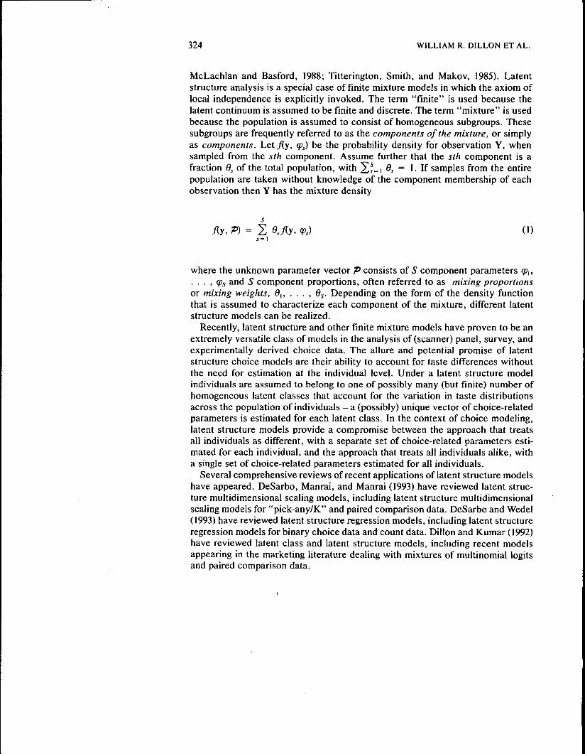
McLachlan and Basford, 1988; Titterington, Smith, and Makov, 1985). Latentstructure analysis is a special case of finite mixture models in which the axiom oflocal independence is explicitly invoked. The term "finite" is used because thelatent continuum is assumed to be finite and discrete. The term "mixture" is usedbecause the population is assumed to consist of homogeneous subgroups. Thesesubgroups are frequently referred to as the components of the mixture, or simplyas components. Let f{y, cp^) be the probability density for observation Y, whensampled from the sth component. Assume further that the sth component is afraction 6, of the total population, with 2]f = i ^̂ = 1 • If samples from the entirepopulation are taken without knowledge of the component membership of eachobservation then Y has the mixture density

Ay, P) = i e,f{y, (p,) (1)

where the unknown parameter vector P consists of S component parameters cp,,. . . , q)s and 5 component proportions, often referred to as mixing proportionsor mixing weights, 6,, . . . , dg. Depending on the form of the density functionthat is assumed to characterize each component of the mixture, different latentstructure models can be realized.

Recently, latent structure and other finite mixture models have proven to be anextremely versatile class of models in the analysis of (scanner) panel, survey, andexperimentally derived choice data. The allure and potential promise of latentstructure choice models are their ability to account for taste differences withoutthe need for estimation at the individual level. Under a latent structure modelindividuals are assumed to belong to one of possibly many (but finite) number ofhomogeneous latent classes that account for the variation in taste distributionsacross the population of individuals - a (possibly) unique vector of choice-relatedparameters is estimated for each latent class. In the context of choice modeling,latent structure models provide a compromise between the approach that treatsall individuals as different, with a separate set of choice-related parameters esti-mated for each individual, and the approach that treats all individuals alike, witha single set of choice-related parameters estimated for all individuals.

Several comprehensive reviews of recent applications of latent structure modelshave appeared. DeSarbo, Manrai, and Manrai (1993) have reviewed latent struc-ture multidimensional scaling models, including latent structure multidimensionalscaling models for "pick-any/K" and paired comparison data. DeSarbo and Wedel(1993) have reviewed latent structure regression models, including latent structureregression models for binary choice data and count data. Dillon and Kumar (1992)have reviewed latent class and latent structure models, including recent modelsappearing in the marketing literature dealing with mixtures of multinomial logitsand paired comparison data.

ISSUES IN THE APPLICATION OF LATENT STRUCTURE MODELS OF CHOICE 325

2. Estimation and computational issues

2.1. ML estimation

A variety of algorithms can be used to find maximum likelihood solutions. Oneapproach is to apply standard numerical optimization methods to the appropriateset of normal equations that define the within-segment conditional densities. Nu-merical methods for obtaining ML estimates primarily involve the use of gradientmethods. Newton-Raphson, quasi-Newton, simplex, and Fisher's scoring aresome of the gradient methods that can be used. Another approach relies on theso-called EM algorithm. In 1977 Dempster, Laird, and Rubin published a seminalpaper describing an algorithm that could be used to obtain ML estimates in avariety of situations. The EM algorithm derives its name from the two basic stepsin the algorithm. In the E-step (expectation step) new provisional estimates of thecomponent membership probabilities (i.e., the posterior probabilities) are ob-tained based upon provisional estimates of 6, and qp,. In the M-step (maximizationstep) new estimates of 6, and % are obtained on the basis of these provisionalestimates of the component membership probabilities. These two steps are re-peated iteratively.

The primary advantages of numerical optimization procedures are their speed,relative to the EM algorithm, and the ability to easily obtain standard errors forparameter estimates - the usual EM algorithm does not directly provide standarderrors. The primary advantages of the EM algorithm are that (1) at each stage inthe iterative process the likelihood is monotonically increasing and (2) under cer-tain regularity conditions, the sequence of likelihoods will converge to at least alocal maximum. Because of its strong convergence properties we favor use of theEM algorithm.

2.2 Identifiability

Problems of identifiability relate to whether unique solutions can be obtained.There are three aspects relating to identifiability that warrant discussion. The firstconcerns whether a distribution or a family of distributions, parameterized interms of one or more natural parameters, is generally identifiable. The secondconcerns the estimation procedure used - whether ML estimation yields identifi-able solutions. And the third concerns the particular response model being fit andthe class of indeterminacies that are relevant.

The evidence suggests that a large number of distributions are identifiable. Al-Hussaini and Ahmad (1981), for example, have shown that the following familiesof multivariate distributions yield identifiable mixtures: negative binomial, loga-rithmic series, Poisson, normal, inverse Gaussian, and random walk. Two excep-tions are the general multivariate normal in which the covariances are treated as


unknown parameters (cf. Hathaway, 1983) and mixed-product multinomials (cf.Haberman, 1977, p. 1135).

An arresting feature of latent structure models is that the likelihood functionneed not be concave. This has two immediate consequences for ML estimation:First, the ML normal equations may fail to maximize the likelihood. Second, mul-tiple maxima of the likelihood may exist: more than one set of ML estimates maymaximize the likelihood. The situation is troubling since the EM algorithm guar-antees convergence only to a local maximum. This means that alternative startingvalues may yield strikingly disparate parameter values. Generally, it will be dif-ficult to prove that a particular latent structure model is identifiable. One heuristicis to investigate whether the matrix of second-order partial derivatives of the log-likelihood is negative definite for the parameter estimates obtained at the maxi-mum. If this condition holds, then the solution corresponds to a local maximumof the likelihood.

Because starting values play a role in the evaluation of whether a solution is aglobal one, how to choose "good" starting values is a question of some concern.The most popular approach to finding starting values is to use the available data.One suggestion is to fit the aggregate model and then use the resulting parameterestimates and associated standard errors to obtain starting values. Another sug-gestion, implemented in much of the work of DeSarbo (see DeSarbo, Manrai, andManrai, 1993, and DeSarbo and Wedel, 1993, for relevant references), is to definestarting values via quick clustering methods using the available data. In manyapplications, such methods have proven to render initial solutions quite close tothe globally optimum solution. Of course, random starting values can always beused. In situations where lack of convergence may be problematic, the use ofrandom start values may be too ambitious, stretching the limits of the algorithmbeyond what is reasonable to expect.

In many latent structure models the natural parameters that define the distri-butional and model form are themselves reparameterized with respect to a set ofcovariates. Depending on the form of the reparameterization, identifiability mayor may not hold. Proper restrictions must be imposed on parameters for identifi-ability to hold for each latent segment. In certain instances, latent structuremodels can help when fitting response models that have known indeterminacies- e.g. unfolding models - by providing a more parsimonious description of thedata that thereby allows both internal and external unfolding models to be fit (cf.Bockenholt and Bockenholt, 1991).

2.3 Determining the number of latent classes/segments

The overwhelming temptation in deciding how many components to retain is tocompute the likelihood ratio statistic between models having S and 5 + 1 com-ponents. Unfortunately, in the case of mixtures the likelihood ratio statistic is not


asymptotically ^^-distributed with known degrees of freedom given by the differ-ence in the number of parameters estimated under the null and alternative hy-potheses. Because of the limitations of the likelihood ratio statistic other alter-natives have been suggested. The following five alternatives have gained somepopularity.

1. One alternative is to use parametric bootstrapping (Hope, 1968). The procedureinvolves drawing T — 1 random Monte Carlo samples of size N from a popu-lation having 5-components and prespecified density, and fitting 5 and 5 + 1component models to each of the generated samples. Anyone that has used thismethod knows all too well that it is extremely costly in terms of machine time.

2. A second alternative is to use information-theoretic-hased model selection cri-teria to assess goodness-of-fit. With this approach the decision on the numberof components to retain proceeds by minimizing a particular information-the-oretic criterion. The oldest of these information criteria measures is AIC(Akaike, 1974). Other criteria include BIC (Schwarz, 1978) and CAIC (Boz-dogan, 1987), which attempt to penalize overparameterization more severelythan does AIC. Though the AIC, BIC, and CAIC have a long history of use,recent simulation studies suggest that they tend to systematically underfit oroverfit depending on sample size and component separation (cf. de Borrero,1993).

3. Bozdogan (1993) developed a new entropic complexity criterion called ICOMP.Similar to AIC, BIC, and CAIC, ICOMP is a penalized information-based va-lidity functional. It can be viewed in terms of two distinct components. Thefirst component measures the lack of fit of the model, and the second compo-nent measures the complexity of the estimated inverse-Fisher information ma-trix. The preliminary evidence on the performance of the ICOMP measure isquite encouraging. More comprehensive and intense simulations are, however,needed before definitive and generalizable conclusions can be drawn.

4. The fourth alternative, introduced by Windham and Cutler (1992), is called theminimum information ratio (MIR). The MIR is the smallest eigenvalue of thematrix F^ ' F, where F is the Fisher information matrix, and F,. is the Fisherinformation matrix for the classified sample. The MIR can be viewed as a mea-sure of the proportion of information about the parameters available withoutknowledge of the subpopulation membership of the sample. The MIR may notat all perform well: see de Borrero (1993) and Cutler and Windham (1993).

5. The fifth alternative represents a very different approach. It involves what iscalled nonparametric ML estimation (NPMLE) (cf. Bohning, Schlattmann, andLindsay, 1992), or what is also is called the flexible support size method since5 itself is treated as an unknown parameter and P is viewed as completelyunknown varying in the set of all probability measures. In essence, withNPMLE a grid of parameter values is specified over which the correspondingpopulation proportions that maximizes the likelihood function are found. Thereare several troubling issues related to the NPMLE approach. First, this ap-


proach is based upon saturating the likelihood with possibly as many points assample observations, which runs contrary to the basic tenet of latent structuremodeling. Second, and perhaps more serious, the algorithms available to dateare for univariate distributions only. Adaptive grid search procedures areneeded in order to extend this approach to multivariate problem settings.

3. Specification and interpretation issues

3.1. Perspectives on heterogeneity

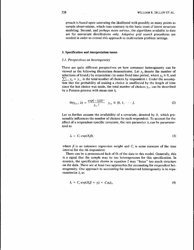
There are quite different perspectives on how consumer heterogeneity can beviewed as the following illustration demonstrates. Let yy denote the number ofselections of brandy by respondent / in some fixed time period, where yy > 0, and2/= I yy = yj+ is the total number of choices by respondent /. Under the assump-tion that the probability of making a choice is unaffected by the length of timesince the last choice was made, the total number of choices yi+ can be describedby a Poisson process with mean rate A,

{ 0 , 1 , • • • , } . ( 2 )3'/

Let us further assume the availability of a covariate, denoted by X, which pre-sumably influences the number of choices by each respondent. To account for theeffect of a respondent-specific covariate, the rate parameter A, can be parameter-ized as

A, = Q exp(;5f,/3), (3)

where /3 is an unknown regression weight and C, is some measure of the timeinterval for the /th respondent.

There can be a pronounced lack of fit of the data to this model. Generally, thisis a signal that the sample may be too heterogeneous for this specification. Inessence, the specification shown in equation 2 may "force" too much structureon the data. There are at least two approaches for accounting for respondent het-erogeneity. One approach to accounting for unobserved heterogeneity is to repa-rameterize A, as

A, = Q txp^Xfi + 7,) = Claiki, (4)


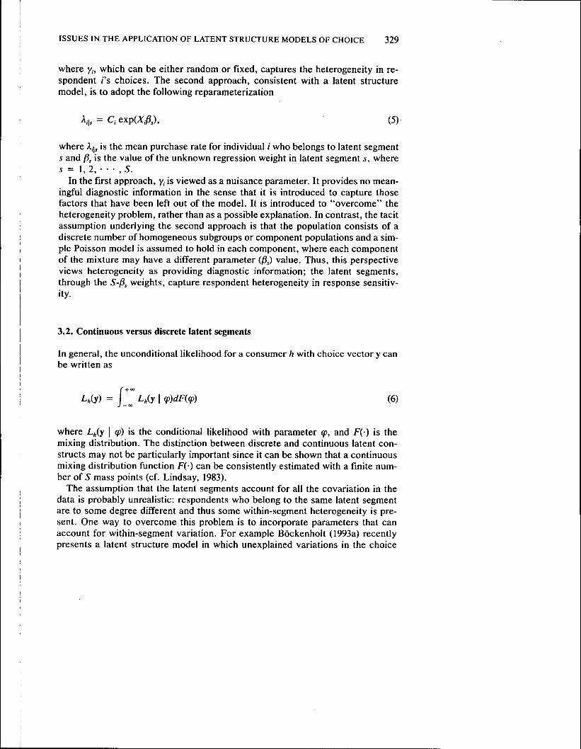
where y,, which can be either random or fixed, captures the heterogeneity in re-spondent /'s choices. The second approach, consistent with a latent structuremodel, is to adopt the following reparameterization

A,|, = C, exp(Z^,), (5)

where A,̂ , is the mean purchase rate for individual / who belongs to latent segments and P, is the value of the unknown regression weight in latent segment s, where5 = 1, 2 , • • • , 5 .

In the first approach, y, is viewed as a nuisance parameter. It provides no mean-ingful diagnostic information in the sense that it is introduced to capture thosefactors that have been left out of the model. It is introduced to "overcome" theheterogeneity problem, rather than as a possible explanation. In contrast, the tacitassumption underlying the second approach is that the population consists of adiscrete number of homogeneous subgroups or component populations and a sim-ple Poisson model is assumed to hold in each component, where each componentof the mixture may have a different parameter (/3j) value. Thus, this perspectiveviews heterogeneity as providing diagnostic information; the latent segments,through the 5-/3̂ weights, capture respondent heterogeneity in response sensitiv-ity.

3.2. Continuous versus discrete latent segments

In general, the unconditional likelihood for a consumer h with choice vector y canbe written as

= f"J - t

(6)

where L^{y \ cp) is the conditional likelihood with parameter (p, and f ( ) is themixing distribution. The distinction between discrete and continuous latent con-structs may not be particularly important since it can be shown that a continuousmixing distribution function F() can be consistently estimated with a finite num-ber of 5 mass points (cf. Lindsay, 1983).

The assumption that the latent segments account for all the covariation in thedata is probably unrealistic: respondents who belong to the same latent segmentare to some degree different and thus some within-segment heterogeneity is pre-sent. One way to overcome this problem is to incorporate parameters that canaccount for within-segment variation. For example Bockenholt (1993a) recentlypresents a latent structure model in which unexplained variations in the choice


probabilities within each latent segment are (potentially) captured by compound-ing the multinomial distribution with the Dirichlet distribution (Johnson and Kotz,1969). Under this specification the choice probabilities vary according to the Dir-ichlet distribution from consumer to consumer within each latent segment and theeffects of covariates are modeled by reparameterizing the Dirichlet parameters.Ramaswamy, Anderson, and DeSarbo (1993) present a mixed NBD model thatcan also account for otherwise unexplained within-segment variation.

4.3. State dependence

When scanner panel data are used to calibrate probabilistic choice models it isgenerally assumed that successive purchases for a household are independent.Latent structure probabilistic choice models are typically parameterized to beconsistent with the proposition that, conditional on latent segment membership,consumers follow a zero-order brand switching pattern. When there is feedback,choice on one occasion affects probabilities of choice on future occasions; somesort of state dependence is operating. State dependence conceivably can manifestseveral different types of behavior. Brand loyalty, as evinced in large repeat pur-chase probabilities, for example, could reflect state dependence: the choice ofalternative A increases the probability of choosing alternative A on the next oc-casion. Similarly, variety seeking could reflect state dependence as well: thechoice of alternative A decreases the probability of choosing alternative A on thenext occasion.

Brand loyalty and brand switching can be distinguished in latent structurechoice models. For example, both Grover and Srinivasan (1987) and Dillon andGupta (1994) advance parametric representations that distinguish between brandloyalty and brand switching. A way of relaxing the zero-order, no feedback as-sumption is to adopt a mixed Markov chain model. Mixed Markov models comeabout by conditioning the choice probabilities by the outcomes of the previouschoice - i.e., outcomes of the previous choices influence the probability distri-bution of the next choice. Thus, in a three-wave problem setting we parameterizethe probability of purchasing brand / on the flrst occasion, brandy on the secondoccasion, and brand k on the third occasion. Mixed Markov models were flrstintroduced by Poulsen (1982). Recently Van de Pol and Langeheine (1989) havemade further advances and provide software for fltting this class of models. Note,however, these models do not consider covariates, so they are somewhat limitedin the amount of diagnostic information provided.

Another example of a latent structure model with state dependence is the flnite-mixture of hazard function models recently suggested by Wedel, Kamakura, andDeSarbo (1993). State dependence is explicitly modeled through a flexible Box-Cox baseline hazard and nonproportional effects of marketing variables, whichare estimated through a flnite-mixture of Poisson regressions.


4.4. Nonstationarity

Stationarity refers to the assumption that consumers do not change their latentsegment membership over time. The assumption of stationarity seems overly re-strictive in at least two ways. First, if consumers are inextricably fixed to a latentsegment, then segments are, by definition, presumed not to grow or diminish overtime. Second, this assumption implies that underlying preference structures mustbe constant and thus are not influenced by marketing mix activity (advertising,promotion), changes in demographics or environmental factors (aging population,weather), politics (changing tax code), etc.

The only nonstationary latent structure probabilistic choice models that haveappeared are due to the work of Poulsen (1982) and extensions by Van de Pol andLangeheine (1989). These models fall under the umbrella of latent Markovmodels. The driving premise underlying these models is that the observed choicesare imperfect indicators, reflecting some measurement or uncertainty, and thatchanges are indeed taking place which cause shifts between the latent states.Thus, at any purchase occasion each consumer is in a particular state; however,over a number of purchase occasions, consumers are allowed to change their la-tent state position. The movement between latent states is governed by a station-ary transition matrix that is conditioned on the present state the consumer is in.Similar to mixed Markov models, latent Markov models have not, to date, beenextended to allow covariates to be included in the parameterization. Finally, alatent structure probabilistic choice model that can account for nonstationarityand state dependence has recently been presented by Bockenholt (1993b).

4.5. Joint versus concomitant specifications

In the context of latent structure probabilistic choice models, there have been twoapproaches to incorporating covariates. One approach includes all covariates inthe specification of the within-segment (conditional) density. Thus, a (possibly)unique within-segment coefficient is estimated for each covariate. The other ap-proach, which has been recently suggested (cf. Dayton and MacReady, 1988; Dil-lon, Kumar, and de Borrero, 1993; Kamakura, Wedel, and Agrawal, 1992), fallsunder the umbrella of concomitant variable modeling. Concomitant variablemodels establish a functional linkage between specific covariates and the priorprobabilities of latent segment membership - the mixing weights.

The rationale behind concomitant variable modeling is that the covariates avail-able are qualitatively different. For example, in the context of choice modeling,one set of covariates typically includes brand-specific variables (price, brand at-tribute ratings), and another set might pertain to respondent-based variables (in-come, family size). The former set of covariates may be thought to influencechoice directly in the sense that they establish the defining character of the latentsegment (a price-sensitive segment, a health-conscious segment, etc.), whereas


the latter set conceivably can be viewed as concomitant variables since they areconceptualized to influence the latent segment membership of a respondent, butare not brand-specific.

5. Future research agenda

We hope the reader will come away with an appreciation of what latent structureprobabilistic models have to offer as well as with heightened sensibilities con-cerning future research issues. Thus, a fitting close to our discussion is to focuson future research priorities:

1. Develop adaptive grid search procedures to implement nonparametric maxi-mum likelihood estimation with multivariate distributions.

2. Identify estimation algorithms that provide high statistical efficiency and lowsearch.

3. Provide comprehensive simulations comparing various methods for determin-ing the number of latent components to retain with particular focus on ICOMPand different methods for computing the Fisher information matrix.

4. Initiate comparative simulation studies focusing on alternative methods forgenerating starting values.

5. Develop latent structure models that can account for consumer heterogeneitycaused by hierarchical data structures.

6. Understand the estimation costs and diagnostic benefits of explicitly specifyinglatent loyalty segments.

7. Develop latent structure models that can incorporate prior information in aBayesian framework.

8. Provide more flexible and comprehensive latent structure probabilistic choicemodels in which consumers are allowed to change latent segment membershipover time as a function of covariates.

9. Develop latent structure probabilistic choice models that relax the zero-orderassumption and parameterize state dependence in terms of a set of covariates.

References

Akaike, H. (1974). "A New Look at Statistical Model Identification," IEEE Transactions on Au-tomatic Control, AC-19, 716-723.

Al-Hussani, E. K., and K. E. Ahmad. (1981). "On the Identifiability of Finite Mixtures of Distri-butions," IEEE Transactions on Information Theory, 27, 664-668.

Bockenholt, U. (1993a). "Estimating Latent Distributions in Recurrent Choice Data," Psycho-metrika, 58. 489-509.

. (1993b). "Latent Change in Recurrent Choice Data," Unpublished manuscript. Depart-ment of Psychology, University of Illinois.


Bockenholt, U., and I. Bockenholt. (1991). "Constrained Latent Class Analysis: SimultaneousClassification and Scaling of Discrete Choice Data," Psychometrika, 56, 699-716.

Bohning, D., P. Schlattmann, and B. G. Lindsay. (1992). "Computer Assisted Analysis of Mixtures(C.A.MAN): Statistical Algorithms," Biometrics, 48, 283-303.

Bozdogan, Hamparsum. (1987). "Model Selection and Akaike's Information Criterion (AIC): TheGeneral Theory and Its Analytical Extensions," Psychometrika, 52, 345-370.

. (1993). "Mixture-Model Cluster Analysis Using Model Selection Criteria and a New In-formational Measure of Complexity." In H. Bozdogan (ed.). Proceedings of the First U.S./JapanConference on the Frontiers of Statistical Modeling, Vol. 2: Multivariate Statistical Modeling.Dordrecht, the Netherlands: Kluwer Academic Publishers.

Cutler, Adele, and Michael P. Windham. (1993). "Information-Based Validity Functional for Mix-ture Analysis." In H. Bozdogan (ed.). Proceedings of the First U.S. Japan Conference on theFrontiers of Statistical Modeling, Vol. 2: Multivariate Statistical Modeling. Dordrecht, theNetherlands: Kluwer Academic Publishers.

Dayton, C. Mitchell, and George B. MacReady. (1988). "Concomitant-Variable Latent-ClassModels," Journal of the American Statistical Association, vol. 83, no. 401, Theory and Meth-ods.

de Borrero, Melinda. (1993). "Determining the Number of Mixture Components and a Poisson-Multinomial Logit Mixture Model Application," Unpublished dissertation. University of SouthCarolina.

Dempster, A. P., N. M. Laird, and D. B. Rubin. (1977). "Maximum Likelihood from IncompleteData via the EM Algorithm," Journal of Royal Statistical Society, B39, 1-38.

DeSarbo, Wayne S., Ajay K. Manrai, and Lalita A. Manrai. (1993). "Latent Class Multidimen-sional Scaling: A Review of Recent Developments in the Marketing and Psychometric Litera-ture," In R. Bagozzi (ed.). The Handbook of Marketing Research. London: Blackwell Publish-ers.

DeSarbo, Wayne S., and Michel Wedel. (1993). "A Review of Recent Developments in LatentClass Regression Models." In Rick P. Bogozzi (ed.). Handbook of Marketing Research, forth-coming.

Dillon. William R., and A. Kumar. (1992). "Latent Structure and Other Mixture Models in Mar-keting: An Integrative Survey and Overview." In Rick A. Bagozzi (ed.). Handbook of MarketingResearch, London: Blackwell Publishers.

Dillon, William R., A. Kumar, and M. Smith de Borrero. (1993). "Capturing Individual Differencesin Paired Comparisons: An Extended BTL Model Incorporating Descriptor Variables," Journalof Marketing Research, 30, 42—51.

Dillon, William R., and Sunil Gupta. (1994). "A Segment-Level Model of Category Volume andBrand Choice," Unpublished manuscript. Southern Methodist University.

Grover, Rajiv, and V. Srinivasan. (1987). "A Simultaneous Approach to Market Segmentation andMarket Structuring," Journal of Marketing Research, 24, 139-153.

Haberman, Shelby J. (1977). "Product Models for Frequency Tables Involving Indirect Observa-tion," Annals of Statistics, 5(6), 1124-1147.

Hathaway, R. J. (1983). "Constrained Maximum Likelihood Estimation fora Mixture of Multivar-iate Normal Densities," Tech. Rep. 92, Deptartment of Mathematics Statistics, University ofSouth Carolina, Columbia, SC.

Hope, A. C. A. (1968). "A Simplified Monte Carlo Significance Test Procedure," Journal of theRoyal Statistical Society, Series B, 30, 582-598.

Johnson, N. L., and S. Kotz. (1969). Distributions in Statistics: Discrete Distributions. New York:Wiley.

Kamakura, Wagner A., Michel Wedel, and Jagdish Agrawal. (1992). "Concomitant Variable LatentClass Models for the External Analysis of Choice Data," Research Memorandum 486, Facultyof Economics, University of Groningen.

Langeheine, R. (1988). New Developments in Latent Class Theory, Latent Trait and Latent ClassModels. New York: Plenum.


Lindsay, B. G. (1983). "The Geometry of Mixture Likelihoods, II: The Exponential Family," An-nals of Statistics, 11,783-792.

McLachlan, G. J., and K. E. Basford. (1988). Mixture Models: Inference and Application to Clus-tering. New York: Marcel Dekker.

Poulsen, C. A. (1982). "Latent Structure Analysis with Choice Modelling Applications." Aarhus:Aarhus School of Business Administration and Economics.

Ramaswamy, V., E. W. Anderson, and W. S. DeSarbo. (1993). "A New Latent Class Methodologyfor Modeling Brand Purchase Frequencies and Deriving Response-Bases Market Segments,"Management Science, 40, 405—417.

Schwarz, G. (1978). "Estimating the Dimension of a Model," Ann Statist, 6, 461-461.Titterington, D. M., A. F. M. Smith, and U. E. Makov. (1985). Statistical Analysis of Finite Mix-

ture Distributions. New York: Wiley.Van de Pol, F., and R. Langeheine. (1989). "Mixed Markov Latent Class Models," Sociological

Methods and Research, 15, 118-141.Wedel, Michel, Wagner A. Kamakura, and Wayne S. DeSarbo. (1993). "Heterogeneous and Non-

proportional Effects of Marketing Variables on Brand Switching: An Application of a DiscreteTime Duration Model," Research Note 541, Faculty of Economics, University of Groningen.

Windham, M. P., and A. Cutler. (1992). "Information Ratios for Validating Mixture Analyses,"Journal of the American Statistical Association, 87(420), 1188-1192.

Documents

Issues in the Estimation and Application of Latent Structure