Embed Size (px)
Citation preview


ISSN 1816-112X
EDITORS-IN-CHIEF Asian Pacific, African and organizing Editor S.L. Chan The Hong Kong Poly. Univ., Hong Kong American Editor W.F. Chen Univ. of Hawaii at Manoa, USA European Editor R. Zandonini Trento Univ., Italy INTERNATIONAL EDITORIAL BOARD F.G. Albermani The Univ. of Queensland, Australia F.S.K. Bijlaard Delft Univ. of Technology, The Netherlands R. Bjorhovde The Bjorhovde Group, USA M.A. Bradford The Univ. of New South Wales, Australia D. Camotim Technical Univ. of Lisbon, Portugal C.M. Chan Hong Kong Uni v. of Science & Technolog y, Hong Kong S.P. Chiew Nanyang Technological Univ., Singapore K.F. Chung The Hong Kong Polyt. Univ., Hong Kong G.G. Deierlein Stanford Univ., California, USA L. Dezi Univ. of Ancona, Italy D. Dubina The Politehnica Univ. of Timosoara, Romania
R. Greiner Technical Univ. of Graz, Austria G.W.M. Ho Ove Arup & Pa rtners Hong Kon g Ltd., Hong Kong B.A. Izzuddin Imperial College of Science, Technology and Medicine, UK J.P. Jaspart Univ. of Liege, Belgium S. A. Jayachandran SERC, CSIR, Chennai, India S. Kitipornchai City Univ. of Hong Kong, Hong Kong D. Lam Univ. of Leeds, UK G.Q. L i Tongji Univ., China J.Y.R. Liew National Univ. of Singapore, Singapore X. Liu Tsinghua Univ., China E.M. Lui Syracuse Univ., USA Y.L. Mo Univ. of Houston, USA J.P. Muzeau CUST, Clermont Ferrand, France D.A. Nethercot Imperial College of Science, Technology and Medicine, UK D.J. Oehlers The Univ. of Adelaide, Australia K. Rasmussen The Univ. of Sydney, Australia T.M. Roberts Cardiff Univ., UK J.M. Rotter The Univ. of Edinburgh, UK C. Scawthorn Scawthorn Porter Associates, USA P. Schaumann Univ. of Hannover, Germany
G.P. Shu Southeast Univ. China J.G. Teng The Hong Kong Polyt. Univ., Hong Kong G.S. Tong Zhejiang Univ., China K.C. Tsai National Taiwan Univ., Taiwan C.M. Uang Univ. of California, USA B. Uy The Univ. of Wollongong, Australia M. Veljkovic Univ. of Lulea, Sweden F. Wald Czech Technical Univ. in Prague, Czech Y.C. Wang The Univ. of Manchester, UK D. White Georgia Institute of Technology, USA E. Yamaguchi Kyushu Institute of Technology, Japan Y.B. Yang National Taiwan Univ., Taiwan B. Young The Univ. of Hong Kong, Hong Kong X.L. Zhao Monash Univ., Australia
Cover: Full scale test for a pre-tensioned truss system under wind pressure. Courtesy of RED Consultant Limited

General Information Advanced Steel Construction, an international journal
Aims and scope The International Journal of Advanced Steel Construction provides a platform for the publication and rapid dissemination of ori ginal and up-to -date research and tec hnological developments in steel c onstruction, design and anal ysis. Scope of research p apers published in this journal includes but is not limite d to theor etical and expe rimental research on elements, assemblages, sy stems, material, design philosophy and codification, standards, fabrication, projects of innov ative nature an d computer tech niques. The journal is specifically t ailored to channel the e xchange of tec hnological know-ho w bet ween r esearchers an d practitioners. Contributions from all aspects related to the recent developments of advanced steel construction are welcome. Instructions to authors Submission of the manuscript. Authors may submit three double-spaced hard copies of manuscripts together with an electronic copy on a diskette or cd-rom in an editable format (MS Word is preferred). Manuscripts should be submitted to the regional editors as follows for arrangement of review.
Asian Pacific , African and organizing editor : Professor S.L. Chan American editor : Professor W.F. Chen European editor : Professor R. Zandonini
All manuscripts submitted to the journal are highl y recommended to accompany with a list of four potential reviewers suggested by the author(s). This list should include the complete name, address, telephone and fax numbers, e mail address, and at least f ive keywords that identify the expertise of each reviewer. This scheme will improve the process of review. Style of manuscript General. Author(s) should provide full postal and email addresses and fax number for correspondence. The manuscript including abstract, keywords, references, figures and tables should be in English with pages numbered and typed with double line spacing on single side of A4 or letter-sized paper. The front page of the article should contain:
a) a short title (reflecting the content of the paper); b) all the name(s) and postal and email addresses of author (s) specifying the author to whom correspondence and proofs
should be sent; c) an abstract of 100-200 words; and d) 5 to 8 keywords.
The paper must contain an introduction and a conclusion. The length of paper should not exceed 25 journal pages (approximately 15,000 words equivalents). Tables and figures. Tables and figures including photographs should be t yped, numbered consecutively in Arabic numerals and with short titles. They should be referred in the text as Figure 1, Table 2, etc. Originally drawn figures and photographs should be provided in a form suitable for photographic reproduction and reduction in the journal. Mathematical expressions and units. The Systeme Internationale (SI) should be followed whenever possible. The numbers identifying the displayed mathematical expression should be referred to in the text as Eq. (1), Eq. (2). References. References to published literature should be referred in the text, in the order of citation with Arabic numerals, by the last name(s) of t he author(s) (e.g. Zandonini an d Zanon [3]) or if more than three authors (e.g. Zandonini et al. [4]) . References should be in English w ith occasional allow ance of 1-2 e xceptional referenc es in local lang uages and r eflect the curren t state-of-technology. Journal titles should be abbreviated in the style of the Word List of Scientific Periodicals. References should be cited in the following style [1, 2, 3]. Journal: [1] Chen, W.F. and Kishi, N., “Semi- rigid Steel Beam-to-column Connections, Data Base and Modellin g”, Journal of
Structural Engineering, ASCE, 1989, Vol. 115, No. 1, pp. 105-119. Book: [2] Chan, S.L. and Chui, P.P.T., “Non-linear Static and Cyclic Analysis of Semi-rigid Steel Frames”, Elsevier Science,
2000. Proceedings: [3] Zandonini, R. a nd Zanon, P ., “Experimental Analy sis of S teel Beams with Semi -rigid Joint s”, Proceedings of
International Conference on Advances in Steel Structures, Hong Kong, 1996, Vol. 1, pp. 356-364. Proofs. Proof will be sent to the c orresponding author to correct an y typesetting errors. Alternations to the original manuscript at this stage will not be accepted. Proofs should be returned within 48 hours of receipt by Express Mail, Fax or Email. Copyright. Submission of an article to “Advanced Steel Construction” implies that it presents the original and unpublished work, and not under consideration for publication nor published elsewhere. On acceptance of a manuscript submitted, the copyright thereof is transferred to th e publisher b y the Transfer of C opyright Agreement and upon t he acceptance of publication for the p apers, the corresponding author must sign the form for Transfer of Copyright. Permission. Quoting from this journal is granted provided that the customary acknowledgement is given to the source. Page charge and Reprints. There will be no page charges if the length of paper is within the limit of 25 journal pages. A total of 30 free offprints will be supplied free of charge to the corresponding author. Purchasing orders for additional offprints can be made on order forms which will be sent to the authors. These instructions can be obtained at the Hong Kong Institute of Steel Construction, Journal website: http://www.hkisc.org The International Journal of Advanced Steel Construction is published quarterly by non-profit making learnt society, The Hong Kong Institute of Steel Construction, c/o Department of Civil & Structural Engineering, The Hong Kong Polytechnic University, Hung Hom, Kowloon, Hong Kong.
Disclaimer. No responsibility is assumed for a ny injury and / or damage to per sons or property as a matter of products liabili ty, negligence or otherwise, or from any use or operation of any methods, products, instructions or ideas contained in the material herein. Subscription inquiries and change of address. Address all subscription inquiries and correspondence to Member Records, IJASC. Notify an address change as soon as possible. All communications should include both old and new addresses with zip codes and be accompanied by a mailing label from a recent issue. Allow six weeks for all changes to become effective. The Hong Kong Institute of Steel Construction HKISC c/o Department of Civil and Structural Engineering, The Hong Kong Polytechnic University, Hunghom, Kowloon, Hong Kong, China. Tel: 852- 2766 6047 Fax: 852- 2334 6389 Email: [email protected] Website: http://www.hkisc.org/ ISSN 1816-112X Copyright © 2006 by: The Hong Kong Institute of Steel Construction.

ISSN 1816-112X
EDITORS-IN-CHIEF Asian Pacific, African and organizing Editor S.L. Chan The Hong Kong Polyt. Univ., Hong Kong American Editor W.F. Chen Univ. of Hawaii at Manoa, USA European Editor R. Zandonini Trento Univ., Italy
VOLUME 3 NUMBER 2 JUNE 2007
Technical Papers Prediction of Top and Seat & Web Angle Connections Cyclic Moment-Rotation Behaviour by a Mechanical Model
530
R. Pucinotti Bases of Design of Overhead Electrical Lines According to General Requirements of European Standard EN 50341-1: 2001
553
Z.K. Mendera Modeling and Analysis of Lattice Towers with More Accurate Models
565
Wenjiang Kang, F. Albermani, S. Kitipornchai and Heung-Fai Lam
Experimental Study of Vrattayata Shape Steel Silo Models 583 N.V. Deshpande and L.M. Gupta Designing Composite Beams with Precast Hollowcore Slabs to Eurocode 4
594
D. Lam Experimental and Theoretical Investigations of Pallet Racks Connections
607
Lucjan Ślęczka and Aleksander Kozłowski

R. Pucinotti 530
PREDICTION OF CYCLIC MOMENT-ROTATION BEHAVIOUR FOR TOP AND SEAT & WEB ANGLE
CONNECTIONS BY MECHANICAL MODEL
R. Pucinotti
Professor, Department of Mechanic and Materials, University of Reggio Calabria, Italy (Corresponding author: E-mail: [email protected])
Received: 13 July 2005; Revised: 19 November 2006; Accepted: 24 November 2006
ABSTRACT: In this paper, a simplified mechanical model of the joint with relative moment-rotation characteristics for use in analytical modelling of MRSF systems is presented. The experimental moment-rotation behaviour of full- scale connections is first considered followed by the development of a finite element model for them. The inelastic moment-rotation predictions of the finite element model are compared with available experimental data. Experimental results of full-scale connections are also compared with the mechanical model proposed by the Eurocode 3. Based on the results of this comparison, a simplified mechanical model of the connection is developed. This proposed simplified mechanical model still adopts the same "component method" approach of the Eurocode 3, but introduces a more refined criteria for the modelling of the unilateral contact between the cleat and the column flange, and a different expression for the evaluation of the joint capacity. An extensive parametric analysis is then conducted to assess the inelastic moment-rotation behaviour and the results are compared with finite element analyses and with available experimental data. The moment-rotation predictions of the simplified mechanical model are in good agreement with experimental tests and with finite element analyses. The simplified mechanical model also gives more consistent initial stiffness and nonlinear relative moment-rotation estimates if compared to the model proposed by the Eurocode 3. The results of the conducted analyses show that the simplified mechanical model gives results that are in reasonable agreement with experimental data and are more accurate than the results of the Eurocode 3-Annex J model.
Keywords: Semi-rigid joints, steel structures, bolted connections, mechanical model, Eurocode 3, Annex J, finite element model, partial strength
1. INTRODUCTION Conventional analysis of frames is usually performed under the assumption that a connection joining beam to column is either infinitely rigid or perfectly pinned. However, experimental test results on full scale joint sub-assemblages (Bernuzzi et al. [1], Calado and Pucinotti [2]) clearly show that the actual response of joints is far from the above idealisation. All connections transmit some moments and exhibit certain degree of flexibility. The unintended modelling error introduces flexibility in the frames and may considerably influence their static and dynamic responses. The concept of semi-rigid connections has been acknowledged by researches several years already. Nowadays, it is well known that all connections are semi-rigid. The concept of semi-rigid or flexible connections is recognized by the Eurocode 3 as well by several national codes for steel structures (for example the U.S.A. codes). But the theoretical knowledge did not actually have an immediate impact on practice. In this paper, the prediction of the cyclic moment-rotation behaviour of top and seat & web angle connections through a simplified mechanical model is presented. Many mechanical models were proposed in the past by the researchers to simulate both monotonic and cyclic behaviour (Kishi and Chen [3], De Stefano et al. [4], Pucinotti [5], Pucinotti [6], Ballio et al. [7] - De Stefano, A. and De Luca [8], De Stefano et al. [4], Bernuzzi et al. [1], Bernuzzi [9], Bernuzzi et al. [10]). The proposed simplified mechanical model is based on the same “component approach” introduced by the Eurocode 3 with an introduction of a more refined modelling of the cleat-to-column interface and a different expression for the evaluation of the moment capacity of the joint, which takes into account for the effect of the d/ta (“d” is the diameter of the bolt connecting the angle to the column
Advanced Steel Construction Vol. 3, No. 2, pp. 530-552 (2007)

Prediction of Top and Seat & Web Angle Connections Cyclic Moment-Rotation Behaviour by a Mechanical Model 531
flange, “ta” is the angle thickness) and ra/ta (“ra” is the groove fillet radius). Finally, the comparison among the experimental curves (Exp.), the Mechanical model (MecMod), the Eurocode 3 Annex J and the “modified” Eurocode 3 Annex J is considered to put in evidence based on their degree of accuracy. 2. THE EUROCODE 3-ANNEX J MODEL The moment-rotation relationships of the connection are non-linear over the entire range of loading for almost all types of joints (Pucinotti, [11]). Different mathematical models have been proposed for the analysis of the inelastic connections behaviour under monotonic loading and under fully reversed cyclic loading (De Stefano and De Luca [8], De Stefano et al. [12], Bernuzzi [13], Bernuzzi et al. [1], Pucinotti [5]). The Annex J of the Eurocode 3 addresses the issue of the analysis and design of beam-to-column joints in building frames subjected to predominantly static loading by the introduction of a mechanical model that simulates the connection behaviour by a series of different components. Each component is being modelled as an elastic spring with a specific stiffness and strength (De Luca et al. [14]). The appropriate coupling of these springs in a parallel-series fashion gives the global stiffness and strength of the connection. Figure 1 shows an example of Annex J model for Top and Seat angle connections. For each type of joint, the component model requires the preliminary identification of the basic components of the joint. Components stiffness coefficients, Ki, and resistant design forces (Frd,i) are then evaluated. Finally, the joint initial rotational stiffness (Sj,ini) and its design moment capacity (Mj,Rd) can be computed. In the case of top and seat angle connections, the EC3 model considers the following components (figure 1b): the stiffness coefficients of the column web panel in: shear (k1), compression (k2) and tension (k3); the column flange flexural stiffness (k4) and the flange cleat flexural stiffness (k6); The bolts tensile stiffness (k10), and, for non-preloaded bolts, their shear stiffness (k11) and their bearing stiffness (k12).
K 1 K 2
K 3 K 6 K 11
K 4 K 10 K 12
a) b)
Figure 1. Example of Annex J model for Top and Seat Angle Connections The initial stiffness of the connection is given by the formula:
∑=
= n
ii
inij
K
EzS
1
2
,
/1 (1)

R. Pucinotti 532
where: E is the Young’s modules, Ki is the stiffness coefficient of the i-th component; n is the number of basic joint components; z is the distance from the mid-thickness of the leg of the angle cleat on the compression flange and
the bolt-row in tension (figure 1b). In the EC3 model, the joint resistance coincides with the resistance of the most weakest component; the flexural joint resistance, Mj,Rd is computed as:
zFM RdRdj =, (2) where:
],...,,min[ 21 RdnRdRdRd FFFF = (3) In EC3-Annex J, the moment-rotation response is described by a linear elastic relationship, Eqn. 4, if the moment Mj,Sd is lower than the elastic one, Me (Me=2/3Mj,Rd ), followed by a non linear part, Eqn. 5, up to the attainment of Mj,Rd, which provides the plateau of the M-F curve up to the ultimate rotation ΦCd (figure 2).
inij
Sdj
SM
,
,=ϕ if RdjSdj MM ,, 3/2< (4)
inij
RdjSdj
SMM
,
,, )/5.1( Ψ
=ϕ if RdjSdjRdj MMM ,,,3/2 << (5)
where: Mj,Rd is the design moment resistance of the connection; Mj,Sd is that applied; Ψ is the shape factor; Sj,ini is the initial stiffens of the connection. The parameter y depends on the joint type (it assumes the value of 3.1 in the case of bolted angle cleats). The Annex J does not include a mechanical model for top-and-seat with web angle connections. An extension of Annex J at this type of connections was presented in ([Pucinotti [5]) (see the curve indicate with EC3 –web in figure 3), where the limitation on the resistance moment was neglected and the validity of Eqn. 5 was extended also to the cases of M>Mj,Rd (indicate with EC3-web+Hr in figure 3):
inij
Sdj
SM
,
,=ϕ if RdjSdj MM ,, 3/2< (6)
inij
RdjSdj
SMM
,
,, )/5.1( Ψ
=ϕ if RdjSdj MM ,, 3/2> (7)

Prediction of Top and Seat & Web Angle Connections Cyclic Moment-Rotation Behaviour by a Mechanical Model 533
ΦEd ΦXd ΦCd Φ
Mj
Mj,Rd
Mj,Sd
Sj,ini
Me
Sh=0
Figure 2. EC3-Annex J Model: Curve M-Φ
EC3 (no web)
EC3 (web)
EC3 (web+Hr)
φ
M
Sj,ini
Sh
Figure 3. Extension of EC3-Annex J Model: Curves M-Φ
3. THE FINITE ELEMENT MODEL To understand the actual behaviour of the available experimental results of this type of connections under monotonic and cyclic loading (Bernuzzi et al. [1]), a finite element model of the test setup has been developed (figure 4). The most relevant parameters influencing the nonlinear response of the joint have been considered in the finite element model. The unilateral contact between the column flange and the angular cleat was modelled with a set of discrete gap elements whose initial stiffness, Kt, was estimated by the following expression (Wales & Rossow [15]) :
ac
wct B
HEtK
)1ln( += (8)
where
twc is column flange thickness; E is Young modulus; Hc is column height; Ba is angle base size.

R. Pucinotti 534
Figure 4. Finite Element Model In figure 5, the finite element model and the Eurocode 3 Annex J model results have been compared with the experimental curves. The same figure 5 shows this comparison with reference to experimental “Bernuzzi” data (Bernuzzi [13]). The results of this comparison (figure 5) show that the finite element moment-rotational predictions are in good agreement with experimental data. The Eurocode 3 model, instead, gives a reasonable estimate of the initial stiffness, but largely underestimates the joint capacity (even including the strain hardening effect). Afterwards, a parametric analysis was developed to understand the influence of most important parameters, in which moment-rotation curves were derived for various values of the varying parameter “d/ta” (where “d” is the diameter of the bolt connecting the angle to the column flange and “ta” is the angle thickness). In figure 6, the results of the finite element model were compared with the inelastic moment-rotation predictions obtained by applying the Eurocode 3-Annex J model. The results of this comparison confirm that the Eurocode 3 underestimates the joint capacity predicted by the finite element model over the entire range of variation of the investigated parameter d/ta. It is possible to see that the EC3, which does not take into account for the effect of the d/ta ratio on the joint capacity, gives inaccurate and conservative results. They confirm that the EC3 model is not accurate enough to assess the inelastic rotation demand of actual connections.

Prediction of Top and Seat & Web Angle Connections Cyclic Moment-Rotation Behaviour by a Mechanical Model 535
TSC-A t=12 d/t=1.7
-100
-50
0
50
100
-30 -15 0 15 30
φ [mrad]
M [kNm]
EC3
TSC-AFEM
TSC-C t=12 d/t=1.7
-100
-50
0
50
100
-30 -15 0 15 30
φ [mrad]
M [kNm]
EC3
TSC-CFEM
TSC-B t=12 d/t=1.7
-100
-50
0
50
100
-30 -15 0 15 30
φ [mrad]
M [kNm]
C
EC3
TSC-BFEM
TSC-D t=12 d/t=1.7
-100
-50
0
50
100
-30 -15 0 15 30
φ [mrad]
M [kNm]
EC3
TSC-DFEM
Figure 5. Comparison among EC3-Annex J model, F.E.M. Model and Experimental “Bernuzzi” Data
d/ta =4
0
10
20
30
0 10 20 30rot [mrad]
M [kNm]
EC3FEM
d/ta =2
0
10
20
30
40
50
60
70
0 10 20 30rot [mrad]
M [kNm]
EC3FEM
d/ta =1.7
0
20
40
60
80
100
0 10 20 30rot [mrad]
M [kNm]
EC3FEM
d/t a =0.8
0
50
100
150
200
250
300
0 10 20 30rot [mrad]
M [kNm]
EC3FEM
Figure 6. Parametric Analysis and Comparison Among F.E.M. Model and EC3-Annex J Model

R. Pucinotti 536
4. THE PROPOSED MECHANICAL MODEL A modified model is proposed in order to improve the inelastic relative moment-rotation predictions of the Eurocode 3. It is still based on the same “component” approach adopted by the Eurocode 3. Using the experimental data and the results of the previous parametric analyses, the model was modified with the introduction of a different expression for the evaluation of the lever arm that modifies the joint capacity. This model is an extension of a previously model (Pucinotti [5]) where the effect of the unilateral contact between the angle cleat and the column flange was already included. The joint is modelled by two rigid bars connected by two non-linear springs (figures 7, 8) that represent the axial response of the angles. The rigid bars AB and CD (figure 7), respectively represent the column and the beam.
A
M
F
F
C
Dδ1
δ2
H
ratfc
L1a
L2ata
dL1
L2
Figure 7. Top and Seat Angle Connections: Mechanical Model
The AC beam, as shown in figure 8, simulates the flexural response of the outstanding leg of angle and the spring BE (figure 8) is introduced to model the bolt behaviour. The AB part of the beam is modelled as an elastic beam supported by a discrete set of independent springs representing the stiffness, Kt , of the column web, Eqn. 8. The segment BC of the beam is modelled as an inelastic beam with linear strain hardening, while the BE segment is modelled as an elastic-perfectly-plastic spring. The end C of the outstanding leg is free to translate vertically, but its rotation is constrained to the value: ϕC= δC Hb , were δC is the vertical translation and Hb is the height of the connected beam. To obtain δC , it is possible to apply the principle of virtual forces (figure 9), considering a virtual unit load condition applied in C and orthogonal to the beam, which gives the moment distribution M’(z):
φ
χδKMM
KNNdzzzM B
Bb
BEL
BEC
a'
0
''2
)()( ++= ∫ (9)
where:
χ = curvature of the part BC of the beam; N’BE =axial load;

Prediction of Top and Seat & Web Angle Connections Cyclic Moment-Rotation Behaviour by a Mechanical Model 537
Kb = axial stiffness of the bolts = fca tt
dE+
4/2π
ta = thickness of the angle; tfc = thickness of the flange column.
C
BA
D
δC
φC
L1
L2
H b
E
Lb
L1
L2
H b
L1a
L2a
Figure 8. Top and Seat Angle Connections: Mechanical Model
A modified expression for the evaluation of “L=L2a” is hereby proposed (figure 8) in order to take into account for the effect of the investigated d/ta ratio and ra/ta ratio (ra=root fillet radius) on the joint capacity:
2/11 dLL a −= (10)
drtLL aaa βα −−−= 22 (11) where: L2, ta ra and d, are shown in figure 7,
⎟⎟⎠
⎞⎜⎜⎝
⎛ +−⎟⎟
⎠
⎞⎜⎜⎝
⎛ ++⎟⎟
⎠
⎞⎜⎜⎝
⎛ +−=
a
aa
a
aa
a
aa
ttr
ttr
ttr 837.10574.9019.2
23
α (12)
and
2/1
4/8)/(3)/(
0
2
=
−+−=
=
β
β
β
aa tdtd
if 1/ <atd if 5.1/1 ≤≤ atd if 5.1/ ≥atd
(13)
The solution of the following fourth order differential equation applied at the part AB of the outstanding leg (figure 8) agrees with the valuation of the rotational stiffness Kφ ?of the spring B:
)()([2 4322112 SACAESACAEEIK −−−= αφ (14)

R. Pucinotti 538
where:
12/3aatBI = ,
)4/1(
4⎟⎠⎞
⎜⎝⎛=
EIKtα , )exp( 11 aLE α= , (15)
)exp( 12 aLE α−= , )cos( 1aLC α= , )sin( 1aLS α= , (16)
in which, A1, A2, A3 and A4, have been carried out by means the boundary conditions:
- bending moment,M(A)=0; - shear, V(A)=0; - horizontal displacement of B, v(B) = −V(B)/Kb; - rotation of B, ϕ (B) = 1
still:
)/(1
31 bdacAA
−== , 412 2 AAA += , baAA /14 −= , (17)
where:
SECESEa 211 2 ++= CECEb 21 += (18)
)(2)(3 21 SCESCEc −+−= αα )(2)( 21 SCESCEd +−−= αα (19) In figure 10, the monotonic non-linear F-δC relationship is reported. On the basis of previous experimental study (Bernuzzi [1,9,10,13]), the response of the outstanding leg in the cyclic case could be defined by the following phases (figure 11):
• unloading phase BC: linear elastic relationship of breadth 2Fe and stiffness Si; CD: post-elastic behaviour with stiffness Sh; DE: contact between the outstanding leg and the column flange;
• reloading phase ED: reloading with contact between the outstanding leg and the column flange; DG: elastic linear relationship of breadth 2Fe and stiffness Si; GH: post-elastic behaviour with stiffness Sh;
The mechanical model in the case of top and seat with web angle connections, presents a number of additional components equal to bolt-rows of the web cleat (figure 12). The stiffness Ktai of the column web (Wales and Rossow [16]) in correspondence of the i-th bolt row is given by the formula:
awic
wctwi B
HEtK
)1ln( += (21)

Prediction of Top and Seat & Web Angle Connections Cyclic Moment-Rotation Behaviour by a Mechanical Model 539
in which:
twc = thickness of the web column; E = Young’s modulus; Hc = height of the beam; Bawi = width of the portion of outstanding leg of web angles (figure 12).
D
B
C
E
φC
Lb δC
H b
L2a
K φ
EK φ
B
C F=1
L.S.D.S.
ABE L1a
K φ
φB=1
Figure 9. Application of the Principle of Virtual Forces
In this case, the extreme C of portion of the outstanding leg of web angle is free to translate horizontally but its rotation ϕCwi = 0.
F
Fe
δe
Fu
δu
Si
Sh
Figure 10. Elasto-plastic Relationship with Linear Strain Hardening

R. Pucinotti 540
F
Fe
2Fe
2Fe
A
B
C
D
E
G
H
Figure 11. Extension at the Cyclic Case
δCwi is obtained by the application of the principle of virtual forces:
wi
BB
bwi
BEL
BECwi KMM
KNNdzzzM
awi
φ
χδ '2
0
''2
)()( ++= ∫ (22)
where:
χ = curvature of the part BC of the beam; N’BE = axial load;
Kbwi = axial stiffness of the bolts = fcaw tt
dE+
4/2π
taw = thickness of the web angle; tfc = thickness of the flange column. Kφwi = rotational stiffness
and:
2/11 dwLL wiawi −= (23)
wwawawwiai dwrtLL βα −−−= 22 (24) where: L1wi and L2wi are depicted in figure 12, while raw is the root fillet radius of web angle and dw is the diameter of web bolts.
⎟⎟⎠
⎞⎜⎜⎝
⎛ +−⎟⎟
⎠
⎞⎜⎜⎝
⎛ ++⎟⎟
⎠
⎞⎜⎜⎝
⎛ +−=
aw
awaw
aw
awaw
aw
awaww t
trt
trt
tr 837.10574.9019.223
α (25)
2/1
4/8)/(3)/(
0
2
=
−+−=
=
w
awwawww
w
tdtd
β
β
β
if 1/ <aww td
if 5.1/1 ≤≤ aww td
if 5.1/ ≥aww td
(26)

Prediction of Top and Seat & Web Angle Connections Cyclic Moment-Rotation Behaviour by a Mechanical Model 541
Baw1
Bawi
Lbw
iδC
wi
A B C
L1w
i
L2w
i
E
Figure 12. Mechanical Model with the Addition of the Web Angles
5. COMPARISON Figures 13 and 14 show the moment-rotation curves obtained by the application of the proposed model, the finite element model and the EC3 model (with and without hardening). The results show that the inelastic rotational predictions of the proposed model are really close to the finite element model. The predictions of the proposed model are more consistent, over the entire range of variation of the investigated parameter “d/t”(0.8÷4), while the results of the Eurocode 3, which do not take into account the effect of the d/ta and r/ta ratios in the evaluation of the lever arm, represent an error. Here, the proposed model is applied to the experimental curves content in the Sericon data bank (Weynand [16]) and to the Bernuzzi experimental tests (Bernuzzi et al. [1]). Figure 15 shows the schemes of the different types of top and seat connections being considered (type A, B and C). Joint type A does not include web angles while joint type B and type C include single web angle connection. The geometric characteristics and the mechanical property of the studied connections are shown in the tables 1, 2 and 3.
Table 1. Bernuzzi: Geometrical and Mechanical Characteristics of the Joints TEST Type of joint Beam Column Flange Angle Type of fya [MPa] fyfc[MPa] fyfb[MPa]
Web Angle Bolt fua[MPa] fufc[MPa] fufb[MPa] TSC-A Type A HE600B IPE300 L120X120X12 M20 313.20 / /
/ 8.8 459.20 / / TSC-B Type A HE600B IPE300 L120X120X12 M20 313.20 / /
/ 8.8 459.20 / / TSC-C Type A HE600B IPE300 L120X120X12 M20 313.20 / /
/ 8.8 459.20 / / TSC-B Type A HE600B IPE300 L120X120X12 M20 313.20 / /
/ 8.8 459.20 / / fya = Yield stress of flange Cleats fyfc = Yield stress of Column flange fyfb = Yield stress of Beam flange fua = Ultimate stress of flange Cleats fufc = Ultimate stress of Column flange fufb = Ultimate stress of Beam flange

R. Pucinotti 542
Table 2. “Sericon” Data Bank: Geometrical and Mechanical Characteristics of the Joints TEST Type of joint Beam Column Flange Angle Type of fya [MPa] fyfc[MPa] fyfb[MPa]
Web Angle Bolt fua[MPa] fufc[MPa] fufb[MPa] 101003 Type A IPE 200 HE160B L150x90x15 M16 / 280.0 351.0
/ - / 422.3 456.0 101006 Type A IPE 200 HE160B L150x90x15 M16 / 280.0 351.0
/ 10.9 / 422.3 456.0 101012 Type A IPE 300 HE160B L150x90x15 M16 / 280.0 303.0
/ 10.9 / 422.3 447.0
Table 3. “Sericon” Data Bank: Geometrical and Mechanical Characteristics of the Joints TEST Type of Beam Column Flange Angle Type of fya[MPa] fyfc[MPa] fyfb[MPa]
joint Web Angle Bolt fua[MPa] fufc[MPa] fufb[MPa]
103001 Type B HE200B IPE 240 L150x90x10 M16 298.0 274.0 291.0 L150x90x10 8.8 478.5 419.0 420.0
103002 Type B HE200B IPE 240 L150x90x10 M16 240.5 274.0 291.0 L150x90x10 8.8 392.0 419.0 420.0
103003 Type B HE200B IPE 300 L150x90x10 M20 298.0 274.0 279.0 L150x90x10 8.8 478.5 419.0 419.0
103004 Type B HE200B IPE 300 L150x90x13 M20 240.5 274.0 279.0 L150x90x13 8.8 392.0 419.0 419.0
103005 Type B HE200B IPE 360 L150x90x10 M24 298.0 274.0 279.5 L150x90x10 8.8 478.5 419.0 418.0
103006 Type B HE200B IPE 360 L150x90x13 M24 240.5 274.0 279.5 L150x90x13 8.8 392.0 419.0 418.0
103045 Type C HE200B IPE 240 L150x90x10 M16 298.0 274.0 291.0 L150x90x10 8.8 478.5 419.0 420.0
103046 Type C HE200B IPE 240 L150x90x13 M16 240.5 274.0 291.0 L150x90x13 8.8 392.0 419.0 420.0
103047 Type C HE200B IPE 300 L150x90x10 M20 298.0 274.0 279.0 L150x90x10 8.8 478.5 419.0 419.5
103048 Type C HE200B IPE 300 L150x90x13 M20 240.5 274.0 279.0 L150x90x13 8.8 392.0 419.0 419.5
103049 Type C HE200B IPE 360 L150x90x10 M24 298.0 274.0 279.5 L150x90x10 8.8 478.5 419.0 418.0
103050 Type C HE200B IPE 360 L150x90x13 M24 240.0 274.0 279.5 L150x90x13 8.8 392.0 419.0 418.0
d/ta =4
0
5
10
15
20
25
30
0 10 20 30rot [mrad]
M [k
Nm
]
F.E.M.EC3MecModEC3 (Hr)
d/ta =2
0
10
20
30
40
50
60
70
0 10 20 30rot [mrad]
M [k
Nm
]
F.E.M.EC3MecModEC3 (Hr)
Figure 13. Comparison among F.E.M. Model, EC3-Annex J Model, Modified EC3- Annex J Model and Mechanical Model
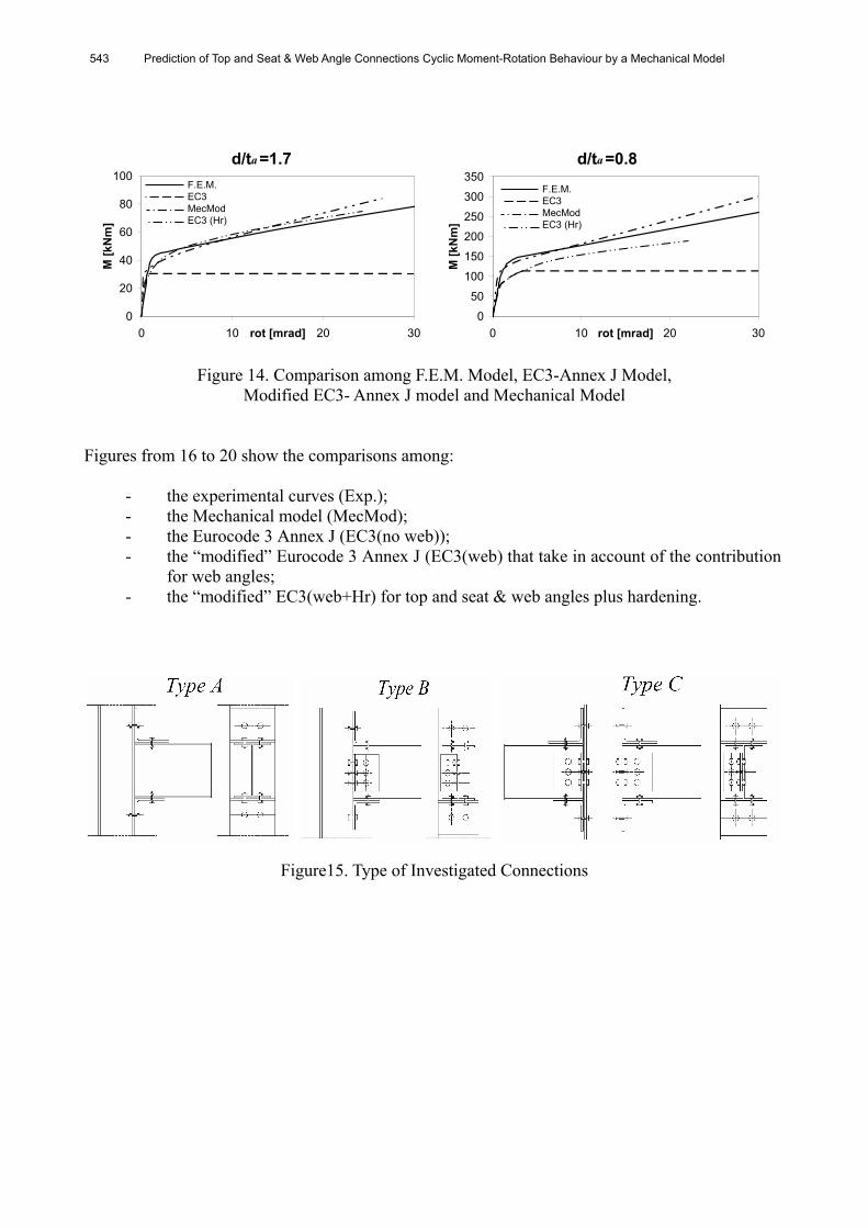
Prediction of Top and Seat & Web Angle Connections Cyclic Moment-Rotation Behaviour by a Mechanical Model 543
d/ta =1.7
0
20
40
60
80
100
0 10 20 30rot [mrad]
M [k
Nm
]
F.E.M.EC3MecModEC3 (Hr)
d/ta =0.8
0
50
100
150
200
250
300
350
0 10 20 30rot [mrad]
M [k
Nm
]
F.E.M.EC3MecModEC3 (Hr)
Figure 14. Comparison among F.E.M. Model, EC3-Annex J Model, Modified EC3- Annex J model and Mechanical Model
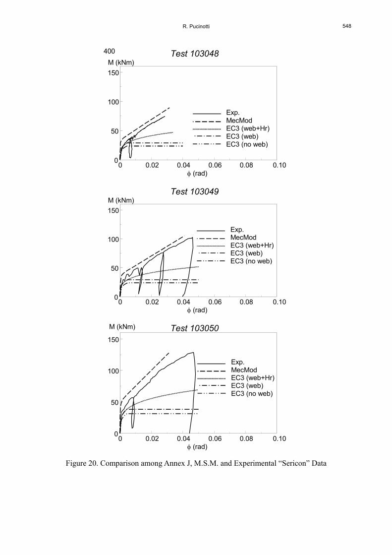
Figures from 16 to 20 show the comparisons among:
- the experimental curves (Exp.); - the Mechanical model (MecMod); - the Eurocode 3 Annex J (EC3(no web)); - the “modified” Eurocode 3 Annex J (EC3(web) that take in account of the contribution
for web angles; - the “modified” EC3(web+Hr) for top and seat & web angles plus hardening.
Figure15. Type of Investigated Connections

R. Pucinotti 544
Test 101003
0 0.02 0.04 0.06 0.08 0.1 0.12 0
40
80
120
φ (rad)
M (kNm)
Exp. MecMod EC3 (Hr) EC3
Test 101006
0 0.02 0.04 0.06 0.08 0.1 0.12 0
40
80
120
φ (rad)
M (kNm)
Exp. MecMod EC3 (Hr) EC3
Test 101012
0 0.02 0.04 0.06 0.08 0.1 0.12 0
40
80
120
φ (rad)
M (kNm)
Exp. MecMod EC3 (Hr) EC3
Figure 16. Comparison among Annex J, M.S.M. and Experimental “Sericon” Data

Prediction of Top and Seat & Web Angle Connections Cyclic Moment-Rotation Behaviour by a Mechanical Model 545
Test 103001
0 0.02 0.04 0.06 0.08 0.10 0
50
100
150
φ (rad)
M (kNm)
Exp. MecMod EC3 (web+Hr)EC3 (web) EC3 (no web)
Test 103002
0 0.02 0.04 0.06 0.08 0.10 0
50
100
150M (kNm)
Exp. MecMod EC3 (web+Hr)EC3 (web) EC3 (no web)
Test 103003
0 0.02 0.04 0.06 0.08 0.10 0
50
100
150
φ (rad)
M (kNm) Exp. MecMod EC3 (web+Hr)EC3 (web) EC3 (no web)
Figure 17. Comparison among Annex J, M.S.M. and Experimental “Sericon” Data

R. Pucinotti 546
Test 103004
0 0.02 0.04 0.06 0.08 0.10 0
50
100
150
φ (rad)
M (kNm)
Exp. MecMod EC3 (web+Hr) EC3 (web) EC3 (no web)
Test 103005
0 0.02 0.04 0.06 0.08 0.10 0
50
100
150
φ (rad)
M (kNm) Exp. MecMod EC3(web+Hr) EC3 (web) EC3 (no web)
Test 103006
0 0.02 0.04 0.06 0.08 0.10 0
50
100
150
φ (rad)
M (kNm)
Exp. MecMod EC3 (web+Hr)EC3 (web) EC3 (no web)
Figure 18. Comparison among Annex J, M.S.M. and Experimental “Sericon” Data

Prediction of Top and Seat & Web Angle Connections Cyclic Moment-Rotation Behaviour by a Mechanical Model 547
Test 103045
0 0.02 0.04 0.06 0.08 0.10 0
50
100
150
φ (rad)
M (kNm) Exp. MecMod EC3 (web+Hr)EC3 (web) EC3 (no web)
Test 103046
0 0.02 0.04 0.06 0.08 0.10 0
50
100
150
φ (rad)
M (kNm) Exp. MecMod EC3 (web+Hr)EC3 (web) EC3 (no web)
Test 103047
0 0.02 0.04 0.06 0.08 0.10 0
50
100
150
φ (rad)
M (kNm) Exp. MecMod EC3 (web+Hr)EC3 (web) EC3 (no web)
Figure 19. Comparison among Annex J, M.S.M. and Experimental “Sericon” Data
R. Pucinotti 548
400
Exp. MecMod EC3 (web+Hr)EC3 (web) EC3 (no web)
Test 103048
0 0.02 0.04 0.06 0.08 0.10 0
50
100
150
φ (rad)
M (kNm)
Test 103049
0 0.02 0.04 0.06 0.08 0.10 0
50
100
150
φ (rad)
M (kNm)
Exp. MecMod EC3 (web+Hr)EC3 (web) EC3 (no web)
Test 103050
0 0.02 0.04 0.06 0.08 0.10 0
50
100
150
φ (rad)
M (kNm)
Exp. MecMod EC3 (web+Hr)EC3 (web) EC3 (no web)
Figure 20. Comparison among Annex J, M.S.M. and Experimental “Sericon” Data

Prediction of Top and Seat & Web Angle Connections Cyclic Moment-Rotation Behaviour by a Mechanical Model 549
The “modified” Eurocode 3 application (top and seat & web cleats, top and seat & web cleats plus hardening) has shown a better accuracy, but it underestimates the resistance and sometimes it overestimates the stiffness. The web cleat’s contribution, in the EC3, produces an increment of the strength about of 10 to 20%. The application of the Eurocode 3, by considering the web cleat plus hardening, shows a better assessment of the actual behaviour of the connections. The mechanical model (MecMod) shows a better evaluation of actual behaviour of the connections, especially on what concerns the prediction of the design moment resistance. The MecMod is able to predict the actual behaviour of different type of connections. The comparison between the moment-rotation curves of mechanical model and the Bernuzzi experimental curves (figures 21, 22, 23 and 24) show a good capability of MecMod on simulating the actual cyclic behaviour of this type of connection. The MecMod, in this first stage, does not take into account the phenomena of stiffness and resistance degradation.
Test TSC-A
-100
-50
0
50
100
-30 -15 0 15 30
φ [mrad]
M [kNm]
Test TSC-A
-100
-50
0
50
100
-30 -15 0 15 30
φ [mrad]
M [kNm]
Figure 21. Comparison among Annex J, MecMod. and Experimental “Bernuzzi” Curve In the same figures, a cycle of mechanical model is compared with an experimental one. It is possible to see the capacity of the model predicting the actual design moment resistance of the investigated connections.

R. Pucinotti 550
Test TSC-B
-100
-50
0
50
100
-30 -15 0 15 30φ [mrad]
M [kNm]
Test TSC-B
-100
-50
0
50
100
-30 -15 0 15 30φ [mrad]
M [kNm]
Figure 22. Comparison among Annex J, MecMod. and Experimental “Bernuzzi” Curve
Test TSC-C
-100
-50
0
50
100
-30 -15 0 15 30
φ [mrad]
M [kNm]
Test TSC-C
-100
-50
0
50
100
-30 -15 0 15 30
φ [mrad]
M [kNm]
Figure 23. Comparison among Annex J, MecMod. and Experimental “Bernuzzi” Curve

Prediction of Top and Seat & Web Angle Connections Cyclic Moment-Rotation Behaviour by a Mechanical Model 551
TSC-D
-100
-50
0
50
100
-30 -15 0 15 30
φ [mrad]
M [kNm]
TSC-D
-100
-50
0
50
100
-30 -15 0 15 30
φ [mrad]
M [kNm]
Figure 24. Comparison among Annex J, MecMod. and Experimental “Bernuzzi” Curve 6. CONCLUSIONS The mechanical model for the inelastic analysis of semi-rigid and partial-strength top and seat angle bolted connections presented was based on the same “component approach” introduced by the Eurocode 3. The Eurocode 3 approach is still maintained, but has been introduced a more refined modelling of the cleat-to-column interface and a different expression for the evaluation of the moment capacity of the joint. It takes into account the effect of d/ta and d/ta ratios. The proposed mechanical model can be included into existing code for the analysis of MRSF, which includes joint types. These conducted analyses yield results in agreement to the experimental data and they are more accurate than the results obtained by the Eurocode 3-Annex J model. REFERENCES [1] Bernuzzi, C., Zandonini, R., Zanon, P., “Experimental Analysis and Modelling of Semi-rigid
Steel Joints under Cyclic Reversal Loading”, Journal of Constructional Steel Research, 1996, Vol. 38, No. 2, pp. 95-123.
[2] Calado, L., Pucinotti, R., “Prove Sperimentali Su Collegamenti Trave-colonna in Acciaio Con Saldatura a Completa Penetrazione”, Departamento de Engenharia Civil, Lisboa Relatorio IC-IST, AI 4, 1996, pp. 251.
[3] Kishi, N. and Chen, W.F., “Moment-rotations of Semi-rigid Connections with Angles”, Journal of Structures Engineering, ASCE, 1990, 116, No. 7, pp. 1813-1834.

R. Pucinotti 552
[4] De Stefano, M.; Bernuzzi, C.; D’Amore, E.; De Luca, A.; Zandonini, R., “Semi-rigid Top and Seat Cleated Connection: a Comparison between Eurocode 3 Approach and Other Formulation”, Proceedings of International Workshop and Seminar on Behaviour of Steel Structures in Seismic Areas, eds. F.M. Mazzolani and V. Goincu (Chapman & Hall, London), 1994b, pp. 568-579.
[5] Pucinotti, R.; “Top and Seat & Web Angle Connections: Prediction via Mechanical Model”, Journal of Constructional Steel Research, 2001a, Vol. 57, No. 6, pp. 663-696.
[6] Pucinotti, R., “Cyclic Mechanical Model for Top and Seat Angle Connections”, XVIII Congresso C.T.A. Venezia, 2001b, Vol. 2, pp. 93-102.
[7] Ballio, G., Calado, L., De Martino, A., Faella, C. and Mazzolani, F.M., “Cyclic Behaviour of Steel Beam-to-column Joints Experimental Research”, Costruzioni Metalliche, 1987, Vol. 2, pp. 69-88.
[8] De Stefano, M. and De Luca, A., “Mechanical Models for Semi-rigid Connections”, Proceedings, First World Conference on Constructional Steel Design, 1992, pp. 276-279.
[9] Bernuzzi, C., “Prediction of the Behaviour of Top-and-seat Cleated Steel Beam-to-column Connections under Cyclic Reversal Loading”, Journal of Earthquake Engineering, 1997, Vol. 2, No. 1, pp. 25-58.
[10] Bernuzzi, C., Calado, L. and Castiglioni, C.A., “Ductility and Load Carrying Capacity Prediction of Steel Beam-to-column Connections under Cyclic Reversal Loading”, Journal of Earthquake Engineering, 1997, Vol. 1, No. 2, pp. 401-432.
[11] Pucinotti, R., “I Collegamenti Nelle Strutture in Acciaio: Analisi Teoriche e Sperimentali”, Thesis for Ph.D. in Structures Engineering of the University of Catania and Reggio Calabria Italy, 1998.
[12] De Stefano M., De Luca A., Astaneh-Asl A, “Modelling of Cyclic Moment-rotation Response of Double-angle Connections”, Journal of Structural Engineering, 1994a, ASCE, Vol. 120, No. 1, pp. 212-229
[13] Bernuzzi, C., Cazzani A. M., Maglitto, M., “Cyclic Response of Components of Steel Connections”, Proceedings of XV Congresso C.T.A., Riva del Garda, 1995, Vol. 2, pp. 108-119.
[14] De Luca, A., De Martino, A., Pucinotti, R. and Puma, G., “(Semi-rigid) Top and Seat Angle Connections: Review of Experimental Data and Comparison with Eurocode 3”, Proceedings of XV Congresso C.T.A., Riva del Garda, 1995, Vol. 2, pp. 315-336.
[15] Wales, M.W.; Rossow, E.C., “Coupled Moment-axial Force Behaviour in Bolted Joints”, Journal of Structural Engineering, ASCE, 1983, Vol. 109, No. 5, pp. 1250-1266.
[16] Weynand, K., “Sericon - Databank on Joints Building Frames”, Proceedings of the 1st COST C1 Workshop, Strasburg, 1992.
[17] Calado, L. and Ferriera, J., “Cyclic Behaviour of Steel Beam-to-column Connections – An Experimental Research”, Proceeding. of Behaviour of Steel Structures in Seismic Areas (STESSA’94) Eds. F.M Mazzolani and V. Gioncu, E & FN Spon, 1994, pp. 381-389.
[18] Commission of the European Communities. Eurocode 3: Design of Steel Structures,1993. [19] Commission of the European Communities. Eurocode 3, Annex j: ENV 1993 – 1 – 1:
1992/A2, 1998. [20] De Stefano, M. and Astaneh, A., “Axial Force-displacement Behaviour of Steel Double
Angles”, Journal of Constructional Steel Research, 1991, Vol. 20, pp. 161-181. [21] Faella, C., Piluso, V. and Rizzano, G., “Structural Steel Semi-rigid Connections – Theory,
Design and Software”. 2000, CRC Press, Boca Raton, Florida, pp. 505. [22] Kishi, N., Chen, W.F., “Database of Steel Beam-to-column Connections”, Structural
Engineering Report, N° CE-STR-86-26, School of Civil Engrg., Purdue University, 1986. [23] Mele, E., Calado, L. and Pucinotti, R., “Indagini Sperimentali Sul Comportamento Ciclico di
Alcuni Collegamenti in Acciaio”, Proceedings of 8th National Conference Earthquake Engineering. ANIDIS, Taormina, 1997, Vol. 2, pp. 1031-1040.

Advanced Steel Construction Vol. 3, No. 2, pp. 553-564 (2007) 553
BASES OF DESIGN OF OVERHEAD ELECTRICAL LINES ACCORDING TO GENERAL REQUIREMENTS OF EUROPEAN
STANDARD EN 50341-1: 2001
Z. K. Mendera
Professor, Department of Civil Engineering, Silesian University of Technology, Gliwice, Poland
(Corresponding author: E-mail: [email protected])
Received: 12 October 2006; Revised: 9 January 2007; Accepted: 18 January 2007 ABSTRACT: Basic requirements about reliability, security and safety conditions of the overhead electrical lines are presented in accordance with European Code EN 50341-1:2001. Actions on overhead lines and load cases on supports have been classified. Basic design assumptions used in analysis of lattice steel towers are announced and limit state method has been consistently introduced to structural design of overhead electrical lines.
Keywords: Overhead electrical line, structural design, limit states, actions on structures, steel supports
1. INTRODUCTION AND ESSENTIAL DEFINITIONS The new European standard EN 50341-1 [1] provides a basis and general principles for the structural, geotechnical and mechanical design of overhead electrical lines in conjunction, in the case of steel structures, with Eurocode 3: EN 1993-1-1 [2] and EN 1993-3-1 [3]. The general principles of structural design are based on the limit state concept used jointly with the partial factor method. The values of the partial factors for actions and material properties depend on the type of structures and the type of limit state. Partial factors also depend on the coordination of strength envisaged for the lines. In principle, there are two approaches used to determine the numerical values for actions, material properties and partial factors of safety. The first one, General approach, is based on the statistical evaluation of meteorological and experimental data and field observations. The second one, Empirical approach, is based on the calibration by a long and successful history of overhead lines construction. In practice, the two above approaches are used in combination. In Poland, according to the National Normative Aspect: EN 50341-3-XX [4], the statistical approach is considered as giving additional, accessible numerical values for actions and material properties to the Empirical approach. In order to achieve a better understanding of the definition of certain terms (by mechanical and electrical engineers), some essential definitions, according to International Electrical Vocabulary – Chapter 466 – Overhead lines: IEC 60050, are presented, as follows:
• Electrical system – all items of equipment, which are used in combination for the generation, transmission and distribution of electricity;
• Mechanical system – set of components connected together to form an overhead electrical line, e.g. conductors, supports, foundations, insulator strings and hardware;
• Electrical reliability – ability of a system to meet its supply function under stated conditions for a given time interval;

554 Bases of Design of Overhead Electrical Lines According to General Requirements of European Standard EN 50341-1: 2001
• Structural reliability – probability that a system performs a given purpose under a set of conditions over a reference period. Reliability is thus a measure of the success of a system in accomplishing its purpose;
• Design working life – assumed period for which a structure is to be used for its intended purpose with anticipated maintenance but without substantial repair being necessary;
• Action – force (load) applied to the mechanical system (direct action) or an imposed deformation caused by temperature changes, uneven settlement, etc. (indirect action);
• Load cases – compatible load arrangements, sets of deformations and imperfections considered simultaneously with defined variable actions and permanent actions for a particular verification;
• Reference period – period taking into account the design working life of the system or of one of its elements and/or of the characteristic value of an action;
• Return period – mean interval between successive recurrences of a climatic action of at least defined magnitude. The inverse of the return period gives the probability of exceeding the action in one year;
• Safety – ability of a system not to cause human injuries or loss of lives during its construction, operation and maintenance;
• Security – ability of a system to be protected from a major collapse (cascading effect) if a failure is triggered in a given component. This may be caused by electrical or structural factors;
• Design situation - set of physical conditions representing a reference period for which the design will demonstrate that the relevant limit states are not exceeded;
• Clearances – distance between two conductive parts along a string stretched the shortest way between these conductive parts; internal clearances – are between phase conductors and earthed parts such as steel structural elements and earth wires and also those between phase conductors; external clearances – are between phase conductors to ground plane, roads, buildings and installations;
• Support – general term for different types of structure that support the conductors of the overhead electrical lines;
• Suspension support – support equipped with suspension insulator sets; • Tension support – support equipped with tension insulator sets; • Tangent support – suspension or tension support used in straight line; • Angle support – suspension or tension support used at angle point of a line; • Section (anchorage) support – tension support with or without a line angle serving
additionally as rigid point in a line to limit cascading; • Terminal (dead-end) support – tension support capable of carrying the total conductor
tensile forces in one direction; • Span length – the horizontal distance between two adjacent supports; • Wind span (of a support) – the arithmetic mean value of the lengths of adjacent spans; • Weight span (of a support) – the horizontal distance between lowest points of conductors on
either side of a support. 2. BASIC REQUIREMENTS An overhead electrical line should be designed and constructed in such a way that during its intended life, it shall perform reliability, security and safety requirements. Moreover, the conditions of the public safety, durability, robustness, maintainability, environmental requirements and appearance of the structure should be considered and found satisfactory.

Z. K. Mendera 555
Reliability requirements are achieved by design according to: EN 50341-1 [1], EN 1990 [6], EN 1991 [7] and EN 1993 [2]. In accordance with the Polish National Aspects EN 50341-3-XX [4], it is decided to apply the reliability level 1 for overhead lines, i.e., the return period T of climatic actions is 50 years. Security requirements correspond to special loads and measures intended to prevent uncontrollable progressive or cascading failures. It is essential that the failure is contained within or very close to the section where overloads occur. In order to prevent cascading failures, some simulated actions and loading conditions are provided. Safety requirements are intended to ensure that construction and maintenance operations do not pose safety hazards to people. The safety requirements consist of all special construction and maintenance loads, taking into consideration the working procedures, temporary guying, lifting arrangement, etc. When designing an overhead line using statistical approach, three different reliability levels may generally be considered, each corresponding to a given return period T of the characteristic value of the variable (climatic) actions:
• level 1 - T = 50 years, • level 2 - T = 150 years, • level 3 - T = 500 years.
Deviations from these levels may be made in accordance with the specific requirements for the project in question. However, the level selected shall at least correspond to a reliability of level 1 (T = 50 years), except for temporary constructions and for components installed temporarily (for example T = 3 or 10 years). The yearly reliability of an overhead line (a structure) is roughly related to the return period T of the climatic actions and is between (1 – 1/T) and (1 – 1/2T), that for reliability level 1 is of 0.98 to 0.99, which can be considered as a minimum value. An absolute reliability of an overhead line (as of each structure) will generally be difficult to determine. Therefore, reliability level 1 can be regarded as the reference reliability whereas the higher reliability levels are to be understood as relative to the reference one. Besides, the reliability of a structure depends on determination of resistance level of the structure. In order to provide an overhead line corresponding to the requirements and to the assumptions made in the design, appropriate quality assurance measures during design and construction should be adopted. Quality assurance is described in EN ISO 9001. The general principles of structural design of overhead line are based on the limit state concept used in conjunction with the partial factor method.
Limit state design shall be carried out by: • setting up structural and load models relevant to ultimate or serviceability limit states,
which are to be considered in various situations and load cases, • verifying that the limit states are not exceeded when design values for actions, material
properties and geometrical data are used in the model.

556 Bases of Design of Overhead Electrical Lines According to General Requirements of European Standard EN 50341-1: 2001
Design values are generally obtained by using characteristic or combination values in conjunction with partial factors, as defined in EN 50341-1 [1], EN-50341-3-XX [4] and in Eurocodes: 0, 1 and 3, i.e. in: EN-1990 [8], EN-1991 [7] and EN-1993-1-1 [2]. Ultimate limit states are those associated with collapse or with other similar forms of structural failure due to loss of stability, overturning, rupture, buckling, etc. Ultimate limit states concern the reliability and security of supports, foundations, conductors and equipment, as well as the public safety. Serviceability limit states correspond to certain defined conditions, beyond which specified service requirements for an overhead line are no longer met. The serviceability requirements concern the mechanical functioning of supports, foundations, conductors and equipment, as well as the electrical clearances. Serviceability limit states include deformations and displacements that affect the appearance of effective use of the support including a reduction of electrical clearances, vibrations which cause damage to conductors, supports or equipment or which limit their functional effectiveness, and the damage which is likely to affect the durability of overhead line. 3. ACTIONS ON OVERHEAD LINES 3.1 Classification of Actions An action, (F), is a direct action, i.e. force (load) applied to the conductors, insulators, supports and foundations or an indirect action, i.e. an imposed or constrained deformation caused, for example, by temperature changes, ground water, variation or uneven settlement, if applicable. Actions may have static or dynamic nature. Usually, with the exception of seismic area, actions on overhead lines are considered as static or quasi-static action, such as wind load, etc. In the design of overhead line supports and foundations, special attention should be paid to the extraordinary span length and slender supports. In view of variation in time, actions on support of overhead lines are classified, as follows: • permanent actions (G), i.e. self-weight of conductors and the effects of the applicable conductor
tension at the reference temperature, self-weight of support foundations, fittings and fixed equipment, as well as uneven settlements of support;
• variable actions (Q), i.e. wind loads, ice loads, conductor tension effects due to wind and ice and temperature and other imposed loads; wind and ice loads as well as applicable temperatures are climatic conditions, which can be assessed by probabilistic methods (general approach) or on a deterministic basis (empirical approach); the vertical reaction from self-weight of the conductor at the support (the weight span) is affected by deviations from the reference state of the conductor tension due to conductor creep and temperature variations and is a variable action. Construction and maintenance loads including working procedures, temporary guying, lifting arrangement, etc., are variable actions with reduced reference period of these actions. Imposed loads arising from conductor stringing, climbing on the towers, etc., are assessed on a deterministic basis and refer to the safety aspect;
• accidental actions,(A), i.e. failure containment loads (at rupture of a conductor); avalanches, exceptional ice loads including unbalanced ice loads, etc. These relate to the security aspect.

Z. K. Mendera 557
Characteristic value of an action, Fk , it is main representative value used for limit state verifications. The characteristic value of permanent action is its mean value, Gk = Gmean . For variable actions, the characteristic value, Qk , corresponds to: either a nominal value used for deterministic based actions and in empirical approach, or an upper value with an intended probability of not being exceeded, e.g. wind and ice loads, during a reference period of one year. In the standard EN 50341-1 (2001), a value of probability 0.02 per year is assumed, i.e. the return period of climatic actions is 50 years for structures of probability level 1 . For accidental actions, representative value is generally a characteristic value, Ak , corresponding to a specified value. Design value of an action, Fd , is expressed in general terms as: Fd = Fk γF , where γF is the partial factor for actions. Combination value of a variable action Q is generally represented as a product of a combination factor and a characteristic value, (ΨQ Qk), or directly by an action with a reduced return period. This combination value is considered to be the design value, to take account of a reduced probability of simultaneous occurrence of the most unfavorable values of several independent actions. Where the occurrence of actions is correlated with each other, this is reflected in the combination factor. In the standard EN 50341-1 [1], the combination factor for a variable action, ΨQ , is principally derived on the basis of a reduced return period and, therefore, includes the partial factor used in the Eurocode format as well as any other reduction factors. Basic design condition of the ultimate limit state is: Ed / Rd ≤ 1 or Ed ≤ Rd, (1) where:
Ed – the total design value of the effect of actions, such as internal force or moment or a representative vector of several internal forces or moments,
Rd – the corresponding structural design resistance associating all structural properties with the respective of structural design values.
3.2 Load Cases The standard load cases are presented in Table 1. For the design of conductors, equipment and supports including foundations in the ultimate limit state load case giving the maximum loading effect in structure and each individual member (and connection) should be considered. Conductor tensions should be determined according to the loads acting on the conductor in the defined load case. The components of the conductor tension at attachment points of the support, including the effects of vertical and horizontal angles, should be taken into account. If, initially, the circuits on a multi circuit support or the sub-conductors of bundles will only be partially installed, this condition shall be considered in the design. Calculations shall be based on the real components of the vertical, transverse and longitudinal loads in various load cases. Weight of towers, conductors and accessories shall be taken into account in all load cases.

558 Bases of Design of Overhead Electrical Lines According to General Requirements of European Standard EN 50341-1: 2001
Table 1. Standard Load Cases Design situation No. Description of a load case (conditions) Temp.
[°C] Apply to
0
Permanent actions of conductors, insulators and supports and foundations
+10 -5 -25 +40
all elements
1 Extreme wind load normal to the line and at all other angles which may be critical to design
+10 -5
all elements
normal
2a Uniform ice load on all spans -5 all elements
2b
Ice loads unbalanced transversely (transverse bending): ice load equal to the characteristic value multiplied by the reduction factor α = 0.5 on all the conductors on all cross-arms on one side only of the support but from other side without a reduction
2c
Ice loads unbalanced longitudinally (longitudinal bending): ice load equal to the characteristic value on all the conductor in one direction only from all cross-arms of the support multiplied by the reduction factor α1 = 0.35 and in the other direction by the reduction factor α2 = 0.7
exceptional (accidental)
2d
Ice loads unbalanced torsionally (torsional bending): ice load equal to the characteristic value on all the conductors on all cross-arms on one side only on the support and in one direction of the line multiplied by the reduction factor α3 = 0.35 but for all remaining conductors multiplied by the reduction factor α4 = 0.7
-5 all supports
normal 3
Combined ice and wind loads, where joined effect Ed should to be determined in two main combinations:
I. Ed = Ed(1,0QIk, 0,4QWk), II. Ed = Ed(0,35QIk, 0,7QWk)
-5 all supports (elements)
4a Actions equal of 2/3 value of one side release of tension in the conductors with uniform ice loads on all spans
tension (anchorage) supports
4b Action of full one-sided release of tension in the conductors with uniform ice load (at the attachment points)
cross-arms and other elements of support on which less than three conductors are tension supported
normal (construction and maintenance)
4c
Construction and maintenance loads appropriately to the method of erection and concentrated loads related to the weight of linesmen, working platform, etc.
-5
all supports
exceptional (accidental) 5
Action equals of full one-sided release of tension in any one earth wires or phase conductors at the attachment point (torsional load)
-5 tension (anchorage) supports
Note: In each load case, it should take into account the permanent actions (No.0), e.g., self-weight of the tower, conductors, insulators, fittings as well as the effect of the applicable conductor tension at the reference temperature. Moreover, in suitable load cases, the conductor tension effect due to wind and ice and temperature deviations from the reference temperature should be taken into consideration.

Z. K. Mendera 559
The main variable actions on conductors, insulators and supports are: wind or icing applied in adequate temperature, as well as combination of wind and ice loads. Wind and ice actions directly on supports (towers) shall also be considered. The following types of supports are distinguished in accordance with their function: • suspension supports and angle suspension supports, ( S and SA), • tension ( anchorage) supports and angle tension(anchorage) supports, ( T and TA), • dead-end (terminal) supports and angle dead-end (terminal) supports, ( D and DA). Security loads are specified to give minimum requirements on the longitudinal and torque resistance of the supports by defining failure containment loads. The loads considered are one-sided release of tension in a conductor and conventional unbalanced overloads (icing), respectively. For control of adequate reliability and functions under service conditions of the overhead line, load cases ought to be defined in the National Normative Aspects (NNA for each European country) to reflect national practices (special national conditions and national complements). In Poland, the NNA: EN 50341-3-XX [4] introduces in formal Empirical approach to define actions on overhead electrical lines, but with the use of statistical data of self-weight of structure components, wind speed and ice loads and limit state format for the design of structures. In practice, the two above approaches are used, i.e. Empirical and General approaches in combination. 3.3 Partial Factors for Actions γF and for Resistance (Material) γM Partial factors for actions, γF, and for resistance, γM, according to EN 50341 -3-XX (2006) are presented in Table 2 and Table 3, respectively.
Table 2. Partial Factors (γF) and Combination Factors (ψF) for Actions Design situation Symbol Factors Normal, construction and maintenance load cases: • Permanent loads • Variable actions (climatic
loads) • Combination of wind and ice
actions
γG γQ, γW, γI ψI and ψW, properly
1.1; (0.9 when favorable) 1.3 1.0 and 0.4 or 0.35 and 0.7
Exceptional load cases: • Permanent loads • Variable actions • Accidental action
γG γQ γA
1.0 1.0 1.0

560 Bases of Design of Overhead Electrical Lines According to General Requirements of European Standard EN 50341-1: 2001
Table 3. Partial Factors for Resistance (γM) Part of structure
Reference limit Kind of resistance of an element Symbol Factor
γM fy Resistance of cross-section γM0 1.0 fy , E Resistance of members to buckling γM1 1.10 fu, fy Resistance of net-section at bolt holes γM2 1.25
Steel supports
fu Resistance of bolted or welded connections γMj 1.25
Resistance with full icing γMCI 1.25 1.40*
Resistance with 50% of icing γMC2 1.90 Resistance in case of III tightening degree γMC3 1.80
Metal conductors
Characteristic resistance Rk Resistance with 50% of icing and in case of
III tightening degree, simultaneously γMC4 2.80
Insulators Guarantee resistance Resistance of insulator γMins 2.00
Fittings Characteristic resistance Resistance of fittings γMf 1.60
Note: (*) if conductor included optical fibres 4. STEEL SUPPORTS (TOWERS) 4.1 Basic Design Assumptions Supports of overhead electrical lines exceeding AC 45 kV are usually designed as lattice steel towers. Exemplary silhouettes of steel towers for high-voltage overhead lines are shown in Figure 1 and pictures of suspension, tension angle and tension transposition supports are shown in Figures 2, 3 and 4, suitably.
Figure 1. Exemplary Silhouettes of Steel Towers for One or Multi-circuit towers of High- and Extra-high Voltage Lines

Z. K. Mendera 561
Figure 2. View of Suspension Support Figure 3. View of Angle Support with Tension Insulator Sets Main assumptions used in global analysis of lattice steel towers are, as follows: • The internal forces and moments in a statically indeterminate structure shall be determined
using elastic global analysis. Lattice steel towers are normally considered as pin jointed truss structures. If the continuity of a member is considered (in a joint point), the consequent secondary bending stresses may generally be neglected. Approximate calculation of member loads by considering tower panels as two-dimensional trusses is acceptable, providing the equilibrium conditions are satisfied. It shall be verified that bracing systems have adequate stiffness to prevent local instability of any parts.
• The internal forces and moments may generally be determined using either first order theory (initial geometry of a structure) or second order theory (actual geometry with the influence of the deformation of the structure). Normally, first order theory is used for the global analysis of self-supporting lattice towers.
• Elastic global analysis shall be based on the assumption that the stress-strain behaviour of the material is linear, whatever the stress level. The assumption may be maintained for both first-order and second-order elastic analyses.
• Three types of lattice steel tower members are considered: main legs and chords, bracings and secondary members (often referred to as redundant members). The secondary members are considered not to be loaded directly by external actions, and the local stability of members carrying loads should be ensured. In the global analysis network, the redundant members can normally be neglected.
• Bending moments due to normal eccentricities are treated in the selection of buckling cases. Bending moments caused by wind loads on individual member are generally negligible, but they need to be considered in the design of slender bracings or horizontal edge members of towers.

562 Bases of Design of Overhead Electrical Lines According to General Requirements of European Standard EN 50341-1: 2001
Figure 4. View of Transposition Support with Tension Insulator Sets
4.2 Design Resistance of Lattice Tower Members Most of lattice tower members are designed by checking their buckling resistance and the proper confession of their effective length (buckling length) and their slenderness is a key question. Until the process of harmonization of the National and European standards is completed, it is possible to use either Polish standard PN-B-03205 [12] with NNA for Poland, EN 50341-3-XX [4], or Annex J of EN 50341-1 [1] for the design of overhead line steel structures in Poland. There are several different configurations of tower members, which are commonly used in lattice towers, and each requires separate consideration about their carrying capacities (resistance). The buckling length, le, and hence the capacity of compression member depends on the type of bracing used to stabilize the member. Generally, according to Eurocode 3 and EN 50341-1-1 [1], checking of buckling resistance of a member is shown below:
ye il=λ or minile=λ - slenderness of the member, (2) where: le = ly or le = lmin – distance between points of the lattice net,
AA
Ef effy
iπλλ = - relative slenderness (slenderness ratio) for flexural buckling;
for angle profiles with equal legs, the relative slenderness for flexural torsional buckling may be calculated approximately using the formula:

Z. K. Mendera 563
AA
Ef
tb effy
pπ
λ 5= ,
Aeff – effective cross-section of the member taking into account the local instability of cross- section.
For members in axial compression, the design value of the compression force, Nd , divided by design value of the buckling resistance, NR,b , shall satisfy the condition: Nd /NR,b ≤ 1, (3) where:
1,
M
yeffbR
fAN
γχ= , (4)
22
1
iλφφχ
−+= - reduction factor (buckling factor) but 1≤χ ,
( ) ]2,01[5,02ii λλαφ +−+= - parameter of buckling curve,
α – imperfection factor depends on accepted buckling curve: a, b, c or d, equal approximately: 0.21; 0.34; 0.49 and 0.76.
Design of the support should be done by calculation only or by calculation validated by a full-scale loading test. If the design is done by calculation only, the appropriate buckling curve to be used shall be the curve c, that is α = 0.49; if design is done by calculation and validated by documented full-scale test , the appropriate buckling curve to be used should be the curve b, that is α = 0.34. Connections should be capable of resisting their applied loads. The resistance of a connection shall be determined on the basis of the resistances of the individual fasteners or welds. Connections are generally considered as nominally pinned. 4.3 Required Electrical Clearances The height of tower, its silhouette and overall dimensions depend on required electrical clearances in detail presented in electrical part of the EN 50341-1 [1]. Guiding information in this range, for the use of steel structures designers, is presented in Table 4.
Table 4. Minimum Air Clearances
Highest system voltage [kV]
Del [m]
Dpp [m]
Clearance to ground [m]
Clearance to trees [m] Clearance to buildings [m]
45/52 0,60 0,70 110/123 1,00 1,15 220/245 1,70 2,00 400/420 2,80 3,20
5 + Del 2,5 + Del Depending on kind of building 2,5 + Del ÷ 10 + Del
Remarks: Del – minimum air clearance required to prevent a disruptive discharge between phase conductors and objects at
earth potential, Dpp – minimum air clearance required to prevent a disruptive discharge between phase conductors. It is not permitted to cross over the apartment buildings, factory buildings, office buildings, etc. by overhead lines exceeding AC 110 kV.
564 Bases of Design of Overhead Electrical Lines According to General Requirements of European Standard EN 50341-1: 2001
5. CONCLUSIONS The new European standard (EN 50341-1 [1]) consistently introduced the limit state concept to structural design (mechanical aspect) of overhead electrical line elements, i.e. conductors, insulators, supports and foundations. The electrical aspect is also taken into consideration, first of all in serviceability limit state, through the requirements of minimum electrical clearances within the span, at the support and to the ground, which have fundamental influence on tower height and cross-arms dimensions. The possibility of combined wind and ice load are considered respective of load cases, as well as unbalanced ice loads on conductors: longitudinally, transversely and torsionally in relation to the tower. These complex requirements based on probabilistic approach (characteristic and design values of the actions and resistances of structures) and empirical approach (realistic load cases and failure cases) increase the reliability of overhead electrical lines. REFERENCES Standards and codes: [1] EN 50341-1, Overhead Electrical Lines Exceeding AC 45 kV – Part 1: General
Requirements - Common Specifications, CENELEC, Brussels, 2001. [2] EN 1993-1-1, Design of Steel Structures, Part 1-1: General Rules and Rules for Buildings,
CEN, Brussels, 2005. [3] EN 1993-3-1, Design of Steel Structures, Part 3-1: Towers, Masts and Chimneys – Tower
and Masts, CEN, Brussels, 2005. [4] EN 50341-3-XX, Overhead Electrical Lines, Part 3-XX: National Normative Aspects for
Poland, PKN, Warszawa, 2006. [5] PN-E-05100-1, Overhead Electrical Lines - Design and Construction, PKN, Warszawa, [in
Polish], 1998. [6] EN 1990, Basis of Structural Design, CEN, Brussels, 2002. [7] EN 1991, Actions on Structures, Parts : 1-1 to 1-6, CEN, Brussels, 2005. [8] EN ISO 9001, Quality Systems, Model for Quality Assurance in Design, Development,
Production, Installation and Servicing, ISO, 2001. [9] IEC 60050 - 466, International Electrical Vocabulary – Chapter 466 – Overhead Lines, IEC. [10] EN 60652, Loading Tests on Overhead Line Structures, CENELEC, Brussels, 2004. [11] PN-90/B-03200, Steel Structures – Design Rules, PKN, Warszawa, [in Polish], 1990. [12] PN-B-03205, Steel Structures, Supports of Overhead Electrical Lines - Design and
Execution, PKN, Warszawa, [in Polish], 1995.

Advanced Steel Construction Vol. 3, No. 2, pp. 565-582 (2007) 565
MODELING AND ANALYSIS OF LATTICE TOWERS WITH MORE ACCURATE MODELS
Wenjiang Kang1 , F. Albermani2 , S. Kitipornchai1 and Heung-Fai Lam1,*
1Department of Building & Construction, City University of Hong Kong,
Hong Kong Special Administrative Region, China *(Corresponding author: E-mail: [email protected])
2Department of Civil Engineering, University of Queensland, Brisbane, Australia
Received: 26 May 2005; Revised: 3 February 2007; Accepted: 14 February 2007
ABSTRACT: In traditional design, transmission towers are assumed to be trusses in the calculation of member axial forces, and secondary braces are usually neglected. However, this assumption does not accurately reflect the structural characteristics of transmission towers. This paper proposes a finite element model (FEM) in which member continuity, the asymmetrical sectional properties of members, the eccentricity of connections, and geometrical and material nonlinearities are considered. The proposed FEM is first verified using experimental results, and is then employed in the analysis of several lattice towers to investigate some of their practical aspects. Recommendations on the design of transmission tower systems are made according to the results of the analysis and given in the conclusion.
Keywords: Transmission towers, secondary bracing, nonlinear analysis, buckling, eccentric connections
1. INTRODUCTION In conventional design, transmission towers are assumed to be trusses [1], and secondary braces are omitted from the analysis. The effects of secondary bracing, eccentric connections, member continuity, and asymmetric member section properties are indirectly considered by modifying a member’s slenderness ratio. With the calculated axial force of the truss model, the member capacity is checked against the relevant column curves that are recommended in the design code, such as the BS standard [2] and the ASCE manual [3]. However, this practice makes the results of the analysis very uncertain. Cannon [4] invited a number of power companies and tower designers to predict the member axial forces and capacities for a typical transmission tower. The coefficients of variation (COVs) in the predicted axial forces of the braces and the main members by different participants were 18.0% and 9.3%, respectively. Even for engineers, who followed the ASCE manual [3], the COV of the predicted capacities was 17.4%. Cannon’s statistics indicate that the predicted capacities of a given transmission tower by the traditional analysis and design method can vary significantly. Many researchers have studied the factors that affect the accuracy of the truss model in the analysis [5-12]. In 1984, Roy et al. [7] investigated the effects of the secondary stresses that arise from joint rigidity and member continuity in the results of analysis. In 1986, Korol et al. [8] reviewed the importance of secondary stresses on the strength of trusses through experiments and parametric analysis. With the full-scale quadrant of a transmission tower panel, Knight and Santhakumar [10] found in 1993 that the effect of joints on the behavior of transmission towers is very great and that the secondary stresses are so significant that they may cause the failure of the leg members. This clearly indicates that the pin-connected truss model is inadequate to represent the real behavior of transmission towers. Robert et al. [12] showed in 2002 that the predicted ultimate strength of a transmission tower is more precise with the continuous beam model than it is with a truss model that was calibrated with full-scale test results.

566 Modeling and Analysis of Lattice Towers with More Accurate Models
To design the load sequence of the full-scale transmission tower test and to find an alternative to the costly full-scale test, Kitipornchai et al. [5] and Albermani and Kitipornchai [6] developed a compact and practical nonlinear method to simulate the global structural response of transmission towers. The program that was developed, the AK-Tower [5, 6], has been employed to predict the behavior of many transmission towers, and its predicted results are in good agreement with the full-scale test results [6]. There is a strong need in the industry to study the behavior of lattice towers intensively. However, research has been directed toward the independent study of structural characteristics. This paper focuses on the development of a finite element model (FEM) that incorporates all of the structural characteristics of lattice towers, such as member continuity, asymmetric section properties, geometric and material nonlinearity, and eccentric connections. Experimental results from the work of Kitipornchai et al. [5] are employed to verify the proposed FEM, which is used with a typical transmission tower panel to study comprehensively the effects of several practical aspects of transmission towers. Design recommendations for these aspects are provided in the conclusion. 2. THE FEM AND ITS VERIFICATION ANSYS, one of the most popular finite element analysis programs, was employed in the study that is reported herein. The BEAM189 element [13] was used to model the angle section. The BEAM189 element automatically provides section-relevant quantities at a number of sections along the structural member. To capture the nonlinearity of the section material, each section is assumed to be an assembly of a predetermined number of nine-node cells. Every angle member is divided into many elements along the longitudinal direction to capture precisely the deformation and to simulate the member’s geometrical nonlinearity. The material nonlinearity of the steel angle section is simulated by the bi-linear model. The nodal degrees of freedom of the connecting members were coupled in specified directions to simulate the connection situations [13]. Furthermore, the connection eccentricity was modeled through the section offset command of ANSYS [13]. Note that the initial geometric imperfection was not included in the FEM. To verify the proposed FEM, the experimentally measured ultimate loads of two angle trusses with different dimensions and member sections (trusses 1 and 2) in Kitipornchai et al. [5], as shown in Figure 1, were employed. Four configurations, which are denoted as 1-OS, 2-OS, 1-SS, and 2-SS, were considered, where 1 and 2 are the truss numbers, and OS (SS) indicates that the free edges of the angle web members are connected on the opposite (same) sides. The dimension L for trusses 1 and 2 is 1000 mm and 750 mm, respectively. As all of the joints are fully welded, all of the connections are assumed to be rigid. Figure 1 shows the FEM of the original and failed trusses. As predicted by the FEM, the failure mode of these trusses was induced by the excessive bending of member 2, primarily in the plane that is perpendicular to the plane of the truss (as in Figure 2(b)), which agrees well with the experimental results in reference 5. TABLE 1 summarizes the calculated results of the proposed FEM and the experimental results [5]. The ultimate load results that were obtained with the proposed FEM were in reasonable agreement with the experimental results. The load-displacement curves of truss 2-OS are shown in Figure 3. The results in TABLE 1 and Figure 3 verify the capability of the proposed FEM. Because the practical yield stress is generally higher than the value that is prescribed by the steel grade, the ultimate load of the practical experiments is consistently higher than that which is predicted by the proposed FEM. The difference is relatively larger for the SS configuration, for which the ultimate loads are larger, than it is for the OS configuration. The small difference between the test and the FEM-predicted results, as shown in Figure 3, may also have been caused by such factors as material strength variance, residual stress, and imperfections, which were not considered in the proposed model.

Wenjiang Kang, F. Albermani, S. Kitipornchai and Heung-Fai Lam 567
Figure 1. The Truss Experiment in Kitipornchai et al. [5]
a) Original FEM
b) Failure Mode of the Truss (Predicted by the FEM)
Figure 2. Failure Mode of the Truss in the 2-OS Configuration, as Predicted by the FEM

568 Modeling and Analysis of Lattice Towers with More Accurate Models
Table 1. Comparison of Test Results: Former and Current Analysis Results
Truss No. 1-OS 2-OS 1-SS 2-SS
Tests [5] 84.4 134.1 139.5 167.2 Ultimate loads, P (kN) Proposed
FEM 71.2 123.5 96.4 152.1
0 2 4 6 8 100
20
40
60
80
100
120
140
160
Truss 2-OS member 2 mid-height out-of-plane deflections
Load
(kN
)
Displacement (mm)
Fiber model [1] Proposed FEM Test results [1]
Figure 3. Comparison of Experimental and Theoretical Load-deflection Curves
3. ANALYSIS RESULTS, COMPARISON AND DISCUSSION Figure 4 shows a typical transmission tower, which is employed as an example for analysis in this study. A typical leg of transmission towers is joined by a heavy splice to another large angle section (stub) that is embedded in the concrete foundation. As a result, the main leg can be modeled as a rigid support in the analysis. Figure 5 shows the physical and analytical models of a typical tower leg.

Wenjiang Kang, F. Albermani, S. Kitipornchai and Heung-Fai Lam 569
(A)
(B)
(C)(D)
(E)
(F)
(G)
(H)
7.42
Leg body
Lower body
Common body
Super structureCross
arm
Cross arm
Figure 4. Full Geometric Model of a Transmission Tower
Horizontals
Secondary bracing elements (redundant)
Main bracing elements (diagonal)
Main leg
Stub
Ground Concrete footing
Panel plane
Bolt
a) Physical Model b) Analytical Model
Figure 5. Physical and Analytical Models for a Typical Transmission Tower Leg

570 Modeling and Analysis of Lattice Towers with More Accurate Models
In general, each plane of a transmission tower is mainly employed to resist in-plane forces and moments. To make the comparison clear without sacrificing its representativeness, the current study focuses on the panel of a transmission tower, as shown in Figure 6. Furthermore, it is assumed that all of the structural members of the transmission tower are formed by angle sections. In the present model, L150 × 150 × 16 mm, L130 × 130 × 10 mm, and L100 × 100 × 6 mm sections are employed for the leg, horizontal, and diagonal members, respectively, and an L70 × 70 × 5 mm section is used for the secondary braces.
H H
V V
Node 1
Node 2
YX
ZY
X
Z
Main bracing elements (diagonal)
Secondary bracing elements (redundant)
Horizontals
Main leg
Node 3
Figure 6. A Panel Model of the Body and Leg for Analysis
3.1 Connection Details To incorporate the eccentric connection details in the model, all of the section properties of the connected angles are transformed to the connection axes. The connection axes for sections 1 and 2 are shown in Figures 7(a) and 7(c). The external loads are assumed to be applied along the corresponding contacting surfaces, as shown in Figure 7(b). Figure 7(d) shows the 3D view of the connection in the proposed FEM.
Section 1
Section 2
Connecting axisY
Updated sectional axis of section 2
Z
C2
Updated sectional axis of section 2 S2S1
Updated sectional axis of section 1
C1
Y
Z Z Z
External Load
a) Offset of Section 1 b) Connection Details c) Offset of Section 2
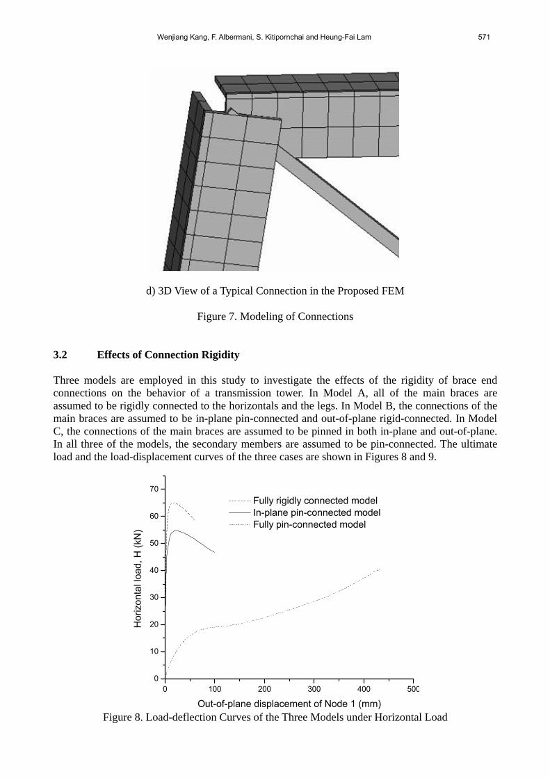
Wenjiang Kang, F. Albermani, S. Kitipornchai and Heung-Fai Lam 571
d) 3D View of a Typical Connection in the Proposed FEM
Figure 7. Modeling of Connections 3.2 Effects of Connection Rigidity Three models are employed in this study to investigate the effects of the rigidity of brace end connections on the behavior of a transmission tower. In Model A, all of the main braces are assumed to be rigidly connected to the horizontals and the legs. In Model B, the connections of the main braces are assumed to be in-plane pin-connected and out-of-plane rigid-connected. In Model C, the connections of the main braces are assumed to be pinned in both in-plane and out-of-plane. In all three of the models, the secondary members are assumed to be pin-connected. The ultimate load and the load-displacement curves of the three cases are shown in Figures 8 and 9.
0 100 200 300 400 5000
10
20
30
40
50
60
70
Hor
izon
tal l
oad,
H (k
N)
Out-of-plane displacement of Node 1 (mm)
Fully rigidly connected model In-plane pin-connected model Fully pin-connected model
Figure 8. Load-deflection Curves of the Three Models under Horizontal Load

572 Modeling and Analysis of Lattice Towers with More Accurate Models
0 50 100 150 200 2500
100
200
300
400
500
600
700
800
Verti
cal l
oad,
V (k
N)
Out-of-plane displacement of Node 2 (mm)
Fully rigidly connected model In-plane pin-connected model Fully pin-connected model
Figure 9. Load-deflection Curves of the Three Models under Vertical Load Figure 8 shows that the connection rigidity has a considerable effect on the ultimate horizontal load capacity. Under the horizontal load, the ultimate load capacities of Models A, B, and C are 65.03 kN, 54.67 kN, and 40.67 kN, respectively. The ultimate load capacity of Model A (in which all of the main braces are rigidly connected) is 19% higher than that of Model B (which is in-plane pin-connected). Furthermore, the ultimate load capacity of Model A is 59.9% higher than that of Model C (which is all pin connected). A similar trend can be observed in the vertical load case, as shown in Figure 9. The failure mode of Model A under horizontal load is shown in Figure 10. Model A fails due to the excessive bending of the main bracing member in the leg, primarily in the plane that is perpendicular to the plane of the truss. Model C also fails for the same reason, but at a much lower ultimate load. Model B has the intermediate ultimate load with a similar failure mode. The failure modes of the three models under vertical load are similar, and one example is shown in Figure 11. Due to the difference in connection rigidity, the displacement curves and ultimate loads are different.

Wenjiang Kang, F. Albermani, S. Kitipornchai and Heung-Fai Lam 573
Figure 10. Failure Mode of Model A under Horizontal Load
Figure 11. Failure Mode of Model A under Vertical Load The above comparison shows that a rigid connection increases the buckling capacity, as was expected. In practice, the assumption of connection rigidity must be realistic; otherwise, we may either overestimate or underestimate the buckling capacity of the structure. The effect of simultaneously applied horizontal and vertical load is also investigated. In the combined load case, the horizontal load (H) and the vertical load (V) are 30kN and 100kN, respectively. The load factor versus the displacement curves is given in Figure 12. The failure mode of the tower under the combined load is illustrated in Figure 13. Under the combined load, the failure modes of the three models vary. However, the effect of the connection rigidity, which can be illustrated by a comparison of the corresponding ultimate loads in Figure 12, is the same as that which is indicated in Figure 8 and Figure 9, and therefore, only the vertical and horizontal load cases are considered in the following sub-sections.

574 Modeling and Analysis of Lattice Towers with More Accurate Models
0 50 100 150 200 250 3000.0
0.2
0.4
0.6
0.8
1.0
1.2
1.4
1.6
1.8
2.0
Load
ing
fact
or
Displacement (mm)
Out-of-plane displacement of Node 3 for fully rigidly connected model
Out-of-plane displacement of Node 1 for in-plane pin-connected model
Out-of-plane displacement of Node 1 for pin-connected model
Figure 12. Load-deflection Curves of the Three Models under the Combined Load
a) Failure Mode of Model A under the Combined Load

Wenjiang Kang, F. Albermani, S. Kitipornchai and Heung-Fai Lam 575
b) Failure Mode of Model C under the Combined Load
c) Failure Mode of Model B under the Combined Load
Figure 13. Failure Modes of the Three Models under the Combined Load
3.3 Effect of Secondary Bracing and its Stress To study the effect of secondary braces, the two models that are shown in Figure 14 are employed. Secondary braces are considered in one model, but are neglected in the other. It turns out that the failure mode for the two models is the same. The load-displacement curves for the two models under horizontal and vertical loads are shown in Figures 15 and 16, respectively.

576 Modeling and Analysis of Lattice Towers with More Accurate Models
XX
ZY
ZY
a) Model with Secondary Bracing b) Model without Secondary Bracing
Figure 14. Analysis Models with and without Secondary Bracing
Figure 15 shows that the ultimate horizontal load capacity of the tower panel with secondary bracing is 65.03 kN, which is much larger than that of the tower panel without secondary bracing (37.32 kN). A similar trend is observed in the vertical load case, which is shown in Figure 16, with an almost 50% increase in ultimate load capacity.
0 50 100 150 200 250 3000
10
20
30
40
50
60
70
Hor
izon
tal l
oad,
H (k
N)
Out-of-plane displacement of Node 1 (mm)
Model without secondary bracing Model with secondary bracing
Figure 15. Load-deflection Curves of Rigid-connected Models under Horizontal Load
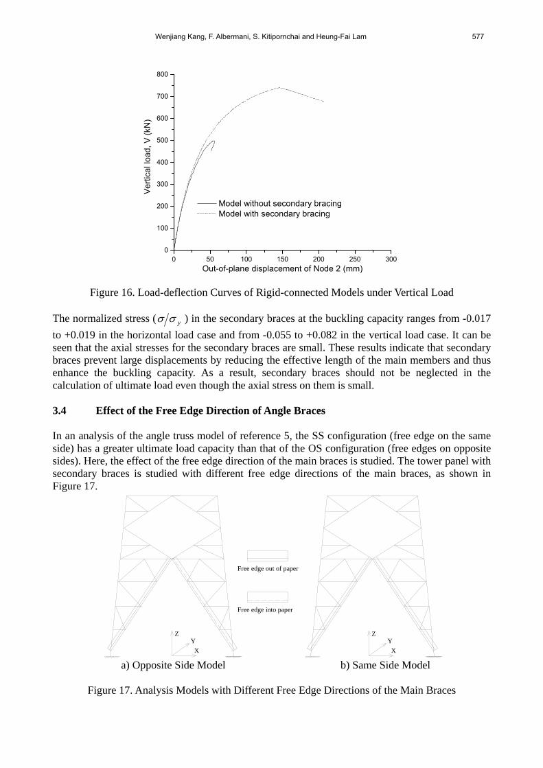
Wenjiang Kang, F. Albermani, S. Kitipornchai and Heung-Fai Lam 577
0 50 100 150 200 250 3000
100
200
300
400
500
600
700
800
Verti
cal l
oad,
V (k
N)
Out-of-plane displacement of Node 2 (mm)
Model without secondary bracing Model with secondary bracing
Figure 16. Load-deflection Curves of Rigid-connected Models under Vertical Load The normalized stress ( yσσ ) in the secondary braces at the buckling capacity ranges from -0.017 to +0.019 in the horizontal load case and from -0.055 to +0.082 in the vertical load case. It can be seen that the axial stresses for the secondary braces are small. These results indicate that secondary braces prevent large displacements by reducing the effective length of the main members and thus enhance the buckling capacity. As a result, secondary braces should not be neglected in the calculation of ultimate load even though the axial stress on them is small. 3.4 Effect of the Free Edge Direction of Angle Braces In an analysis of the angle truss model of reference 5, the SS configuration (free edge on the same side) has a greater ultimate load capacity than that of the OS configuration (free edges on opposite sides). Here, the effect of the free edge direction of the main braces is studied. The tower panel with secondary braces is studied with different free edge directions of the main braces, as shown in Figure 17.
X
Z
Free edge out of paper
Free edge into paper
Y YZ
X a) Opposite Side Model b) Same Side Model
Figure 17. Analysis Models with Different Free Edge Directions of the Main Braces

578 Modeling and Analysis of Lattice Towers with More Accurate Models
Due to the difference in angle directions, the failure mode is caused by the excessive bending of the leg member, as shown in Figure 18. When this failure mode is compared to the one in Figure 10 (for SS configuration), the bending directions of the failed member in the two models are different. The calculated out-of-plane displacement of node 2 (as indicated in Figure 6) for both the OS and SS configurations under horizontal and vertical loads are shown in Figures 19 and 20, respectively. As shown in the two figures, the leg free edge direction has significant effects under horizontal load, but has a very small effect under vertical load. Furthermore, the SS configuration performs better than the OS configuration, which happens to be very popular in transmission tower construction.
Figure 18. Failure Mode of Rigid Model with OS Configuration under Horizontal Load
0 50 100 150 200 250 3000
10
20
30
40
50
60
70
Hor
izon
tal l
oad,
H (k
N)
Out-of-plane displacement of Node 1 (mm)
OS model with secondary bracing SS model with secondary bracing
Figure 19. Load-deflection Curves of Node 2 with Secondary Bracing under Horizontal Load

Wenjiang Kang, F. Albermani, S. Kitipornchai and Heung-Fai Lam 579
0 50 100 150 200 250 3000
100
200
300
400
500
600
700
800
Ver
tical
load
, V (k
N)
Out-of-plane displacement of Node 2 (mm)
OS model with secondary bracing SS model with secondary bracing
Figure 20. Load-deflection Curves of Node 2 with Secondary Bracing under Vertical Load
3.5 Effects of Secondary Bracing Configurations Here, the effects of various secondary bracing configurations on buckling capacity are studied. Five secondary bracing configurations, as shown in Figure 21, are considered in this study. The SS configuration with rigid connections is employed in all of the models in Figure 21.
(A) (B) (C) (D) (E)
Figure 21. Secondary Bracing Configurations
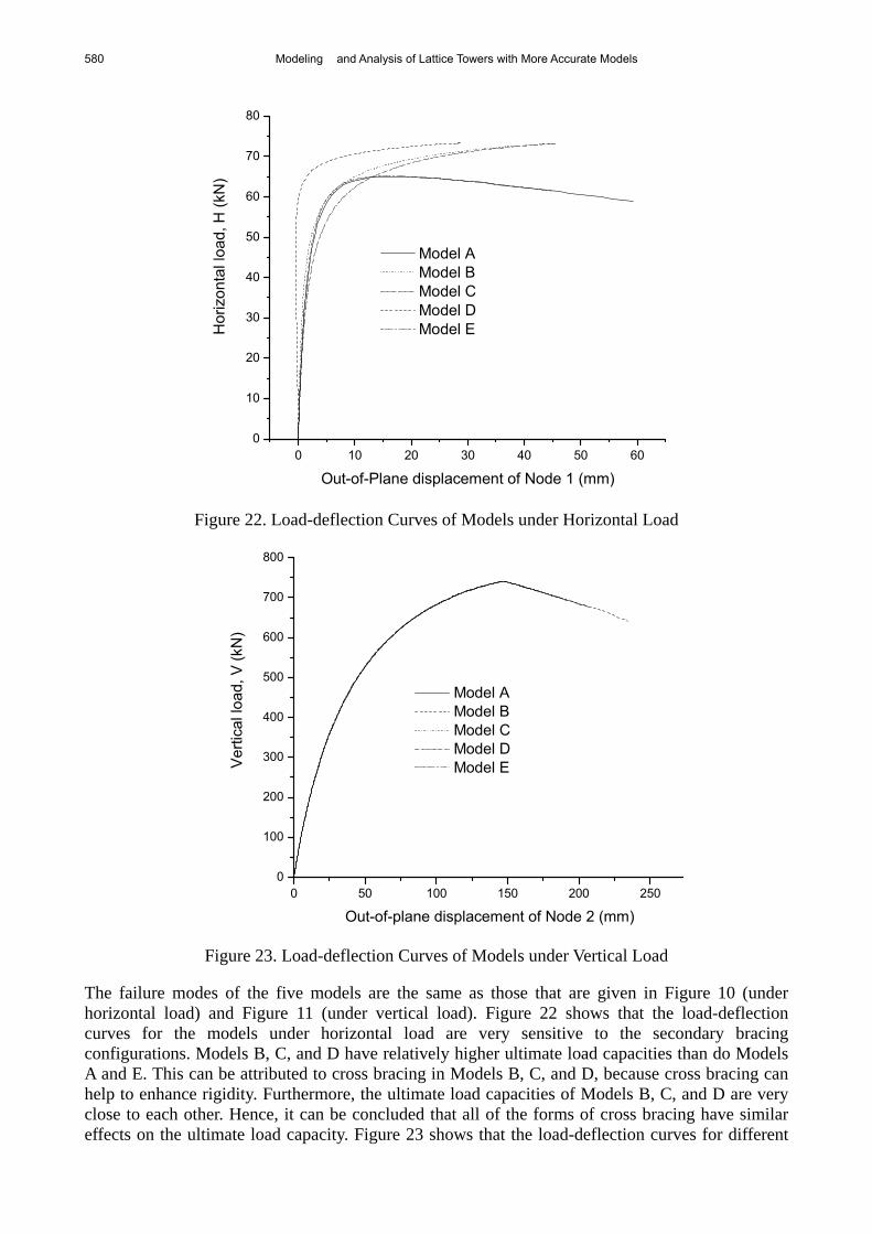
580 Modeling and Analysis of Lattice Towers with More Accurate Models
0 10 20 30 40 50 600
10
20
30
40
50
60
70
80
Hor
izon
tal l
oad,
H (k
N)
Out-of-Plane displacement of Node 1 (mm)
Model A Model B Model C Model D Model E
Figure 22. Load-deflection Curves of Models under Horizontal Load
0 50 100 150 200 2500
100
200
300
400
500
600
700
800
Ver
tical
load
, V (k
N)
Out-of-plane displacement of Node 2 (mm)
Model A Model B Model C Model D Model E
Figure 23. Load-deflection Curves of Models under Vertical Load
The failure modes of the five models are the same as those that are given in Figure 10 (under horizontal load) and Figure 11 (under vertical load). Figure 22 shows that the load-deflection curves for the models under horizontal load are very sensitive to the secondary bracing configurations. Models B, C, and D have relatively higher ultimate load capacities than do Models A and E. This can be attributed to cross bracing in Models B, C, and D, because cross bracing can help to enhance rigidity. Furthermore, the ultimate load capacities of Models B, C, and D are very close to each other. Hence, it can be concluded that all of the forms of cross bracing have similar effects on the ultimate load capacity. Figure 23 shows that the load-deflection curves for different

Wenjiang Kang, F. Albermani, S. Kitipornchai and Heung-Fai Lam 581
models under vertical load are almost the same. This is because buckling under vertical load is induced by the horizontal members, whereas buckling under horizontal load is induced by the leg members, for which the secondary braces make a significant contribution to the behavior of the system. 4. CONCLUDING REMARKS A finite element model (FEM), which considers member continuity, asymmetrical sectional properties, the eccentricity of connections, and geometrical and material nonlinearities, is proposed and was verified by experimental data from the literature [5]. A series of comprehensive parametric studies were then carried out with the proposed FEM. Referring to the results of the analysis, the following conclusions are made.
1. The connection rigidity of the main braces should be considered when calculating the ultimate load capacity of a tower, as it has significant effects on the buckling capacity of the overall structural system. Inappropriate modeling of the connection rigidity may overestimate or underestimate buckling capacity.
2. Although secondary braces are usually subjected to very small axial loads, the results show that their existence greatly enhances the buckling capacity of the structure by reducing the effective length of the leg members. Nonlinear analysis without consideration of secondary braces may lead to an unreliable prediction of the ultimate load capacity of the system.
3. The free edge direction of the main braces has significant effects on the buckling capacity of transmission towers in certain cases. The SS configuration performed better than the OS configuration did in the example that was used in this paper. In a calculation of the ultimate load capacity of transmission towers, a consideration of the effect of free edge directions in the FEM is strongly recommended.
4. The results of the analysis also show that cross bracing in the secondary bracing configuration can enhance the ultimate load capacity of the structure. Furthermore, the case study also shows that different types of cross bracing configurations provide a similar enhancement of buckling capacity.
REFERENCES [1] Marjerrison, M., “Electric Transmission Tower Design,” Journal of the Power Division,
ASCE, 1968, Vol. 94(PO1), pp. 1-23. [2] British Standards Institution, “BS8100: Part 3. Lattice Towers and Masts: Code of Practice
for Strength Assessment of Members of Lattice Towers and Masts,” 1999, London, UK. [3] American Society of Civil Engineers, “ASCE 10-97: Design of Latticed Steel Transmission
Structures,” 1998, New York, USA. [4] Cannon, D.D.J., “Variation in Design Practice for Lattice Towers,” Proceedings of the
Sessions related to Steel Structures at Structures Congress of ASCE, San Francisco, CA, USA, 1989, pp. 268-277.
[5] Kitipornchai, S., Albermani, F.G.A. and Chan, S.L., “Elasto-plastic Finite Element Models for Angle Steel Frames,” Journal of Structural Engineering, ASCE, 1990, Vol. 116, No. 10, pp. 2567-2581.
[6] Albermani, F.G.A. and Kitipornchai, S., “Non-linear Analysis of Transmission Towers”, Engineering Structures, 1992, Vol. 14, No. 3, pp. 139-151.
[7] Roy, S., Fang, S.J. and Rossow, E.C., “Secondary Stresses on Transmission Tower Structures,” Journal of Energy Engineering, 1984, Vol. 110, No. 2, pp. 157-174.

582 Modeling and Analysis of Lattice Towers with More Accurate Models
[8] Korol, R.M., Rutenberg, A. and Bagnariol, D., “On Primary and Secondary Stresses in Triangulated Trusses,” Journal of Constructional Steel Research, 1986, Vol. 6, No. 2, pp. 123-142.
[9] Rao, N.P. and Kalyanaraman, V., “Non-linear Behaviour of Lattice Panel of Angle Towers”, Journal of Constructional Steel Research, 2001, Vol. 57, No. 12, pp. 1337-1357.
[10] Knight, G.M.S. and Santhakumar, A.R., “Joint Effects on Behavior of Transmission Towers,” Journal of Structural Engineering, ASCE, 1993, Vol. 119, No. 3, pp. 698-712.
[11] Kemp, A.R. and Behncke, R.H., “Behavior of Cross-bracing in Latticed Towers,” Journal of Structural Engineering, ASCE, 1998, Vol. 124, No. 4, pp. 360-367.
[12] Robert, V. and Lemelin, D.R., “Flexural Considerations in Steel Transmission Tower Design,” Proceedings of the “Electrical Transmission in a New Age” Conference of ASCE, Omaha, Nebraska, USA, 2002, pp. 148-155.
[13] ANSYS Inc., ANSYS Structural Analysis Guide.

Advanced Steel Construction Vol. 3, No. 2, pp. 583-593 (2007) 583
EXPERIMENTAL STUDY OF VRATTAYATA SHAPE STEEL SILO MODELS
N.V. Deshpande1,* and L.M. Gupta2
1Assistant Professor, Department of Civil Engineering,
K.I.T.S., Ramtek - 441106 (M.S.), INDIA *(corresponding author: E-mail : [email protected])
2Professor, Department of Applied Mechanics, VNIT, Nagpur (M.S.), INDIA E-mail : [email protected]
Received: 26 May 2006; Revised: 27 October 2006; Accepted: 7 November 2006
ABSTRACT: Silos are the tall containers used to store bulk solids. The circular and rectangular shapes of silo containers are common in use. The vrattayata shape for silo containers resembles like an elongated circle. It is formed by connecting two semicircular walls of same radius with straight walls. The length of straight walls is kept as less as possible to minimize the effect of bending stresses. The behaviour of vertical walls of three such vrattayata silo models and that of one circular silo model are experimentally investigated. The volume enclosed within vertical walls of all silo models is kept unchanged to have the same capacity. The inferred static horizontal pressures from measured strains are compared with predictions by Reimbert’s theory and by the method recommended in Euro Code 1 Part 4. The results obtained are discussed and conclusions are drawn.
Keywords: Silo; circular; vrattayata; reimbert’s theory; stress; strain
1. INTRODUCTION Many investigators all around the globe have conducted experiments to measure silo pressures and frictional wall loads to examine the validity of generally accepted design assumptions as incorporated into silo-design codes and procedures. These experiments have been carried out on circular and rectangular shapes of model silos as well as full size silos. Lenczner [1] conducted experiments on model silo and found that the ratio of lateral pressure to vertical pressure instead of being constant as assumed in Janssen’s theory, varied almost linearly with depth. Garg and Gopalkrishnan [2] in their experimentation on square silo model found that the lateral and frictional wall loads during filling and during emptying were higher than those predicted by IS4995-1968. Blight [3] found that horizontal pressures due to stored coarse material were not necessarily radially uniform as assumed in theory. Blight [3] reported about the interpretation of strain measurements on steel silos for computing inferred horizontal pressures and inferred frictional wall loads. Reimbert’s theory for silo loads is a result of mathematical interpretation of the law of hyperbolic distribution of pressures that is closely possible to the reality and includes various parameters appertaining both to the ensiled material and to the dimensional characteristics of silos. Janssen’s theory accepts the hypothesis of constant value of ratio of horizontal thrust to vertical pressure in the interior of silos. Variation of this ratio is taken into account by Reimbert’s Theory.

584 Experimental Study of Vrattayata Shape Steel Silo Models
2. DEVELOPMENT OF CONCEPT 2.1 Vrattayata Shape The wall of circular silo is subjected to hoop tension due to lateral pressure exerted by the stored material in silo leading to the development of uniform axial tensile stresses in wall cross-section at a particular depth. The walls of square or rectangular silos are subjected to horizontal bending stresses predominantly due to lateral pressure exerted by stored material in silo at a particular depth requiring more wall thickness. Vrattayata shape, resembling like an elongated circle, is a combination of semicircular walls and straight walls. Due to the lateral pressure exerted by stored material, semicircular walls are predominantly subjected to hoop tension and straight walls are subjected to bending moments. When the length of straight wall is reduced to a feasible level, the bending moments will also reduce.
Figure 1. Circular and Vrayattayata Shapes 2.2 Geometrical Properties The Geometrical properties of storage container used in the silo theory are the cross-sectional area, the perimeter, the hydraulic radius, the height of wall, the volume of storage. The expressions for these properties are shown in Table 1 for circular and Vrattayata shapes.
Table 1. Expressions for Geometrical Properties of Circular and Vrattayata Shapes Shapes S.
No. Property Circular Vrattayata
1 Straight wall length (L) - xrv 2 Cross sectional Area (A) 2
cc rA π= ( )x2rA 2vv +π=
3 Perimeter (U) Uc = 2 π rc Uv = 2 rv (π+x)
4 Hydraulic Radius (R) Rc = 0.5 rc ( )( )x
x2r5.0R vv +π+π
×=
5 Height of wall (H) 2c
c rVHπ
= ( )x2rVH 2
vv +π=
CIRCULAR
cr
VRAYATTAYATA
vrv r
L
rvL = x

N.V. Deshpande and L.M. Gupta 585
3. EXPERIMENTAL INVESTIGATION 3.1 Models – Dimensions and Geometrical Properties The internal volume enclosed within vertical walls of all models is kept unchanged. The height to diameter ratio of basic circular silo model ‘C’ is Two. The dimensions of vrattayata silo models are calculated for x = 0.2 and based upon the approaches as shown in Table 2.
Table 2. Vrattayata Silo Models Selected for Experimental Study Sl. No. Model Referred Approach Property
1 V12 I Uv = Uc 2 V22 II Av = Ac 3 V32 III Rv = Rc
24 Gauge B.P. sheets having average thickness of 0.6 mm are used in fabrication of all models. Table 3 shows dimensions of all models.
Table 3. Dimensions of Models Sl. No. Model rc (mm) rv (mm) L (mm) Hc (mm) Hv (mm)
1 C 250.0 - - 1000 - 2 V12 - 235.0 47.0 - 1004 3 V22 - 235.4 47.0 - 1000 4 V32 - 236.0 47.2 - 997
3.2 Properties The modulus of elasticity of wall material is found to be 1.1 x 10⁸ kN/m2 while the Poisson’s Ratio is 0.38. The river bed dry sand passing through 4.75 mm IS sieve and retained on 1.18 mm IS sieve is used as stored material in all the models for the present experimental work. This sand has bulk density of 17 kN/m3, mean angle of internal friction as 42.720 and mean angle of friction against wall plates as 28.280. 3.3 Instrumentation The instrumentation consists of electrical resistance strain-gauges, dummy strain gauge, digital strain meter and 20 channel box. A pair of strain-gauge consisting of one horizontal and one vertical strain-gauge is pasted in all model walls at pre-determined locations. These locations of strain-gauges measured from top are the same for all models. On vrattayata silo models, the strain-gauges are pasted on curved and straight surfaces of walls. The strain gauges used are of Type BKCT 20 with gauge length 20 mm and have resistance 119.2 ± 0.2 ohms. 3.4 Recording of Strains The strains in all models are recorded when the sand is fully filled in the models. Tables 4 to 7 show the strains observed on curved and straight surfaces of walls of all models. Experimental set up is shown from Figures 2 to 4.
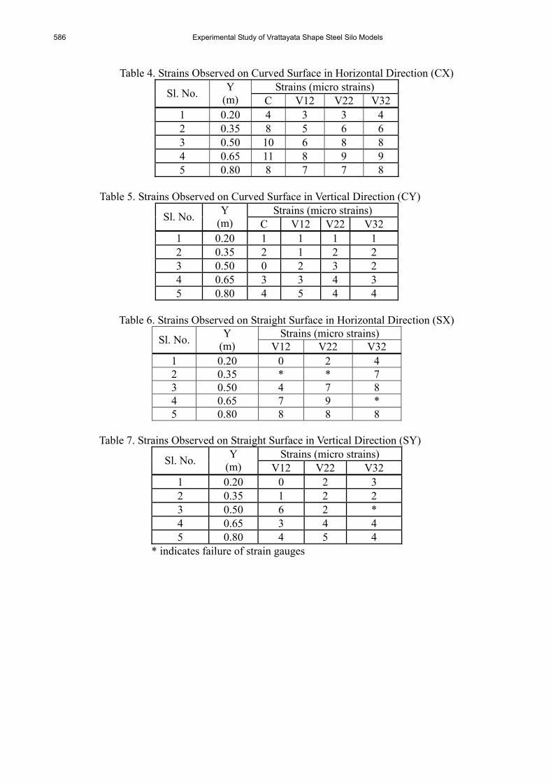
586 Experimental Study of Vrattayata Shape Steel Silo Models
Table 4. Strains Observed on Curved Surface in Horizontal Direction (CX) Strains (micro strains) Sl. No. Y
(m) C V12 V22 V32 1 0.20 4 3 3 4 2 0.35 8 5 6 6 3 0.50 10 6 8 8 4 0.65 11 8 9 9 5 0.80 8 7 7 8
Table 5. Strains Observed on Curved Surface in Vertical Direction (CY)
Strains (micro strains) Sl. No. Y (m) C V12 V22 V32
1 0.20 1 1 1 1 2 0.35 2 1 2 2 3 0.50 0 2 3 2 4 0.65 3 3 4 3 5 0.80 4 5 4 4
Table 6. Strains Observed on Straight Surface in Horizontal Direction (SX)
Strains (micro strains) Sl. No. Y (m) V12 V22 V32
1 0.20 0 2 4 2 0.35 * * 7 3 0.50 4 7 8 4 0.65 7 9 * 5 0.80 8 8 8
Table 7. Strains Observed on Straight Surface in Vertical Direction (SY)
Strains (micro strains) Sl. No. Y (m) V12 V22 V32
1 0.20 0 2 3 2 0.35 1 2 2 3 0.50 6 2 * 4 0.65 3 4 4 5 0.80 4 5 4
* indicates failure of strain gauges

N.V. Deshpande and L.M. Gupta 587
Figure 2. Marking of Strain-gauges
Figure 3. Silo Model Filled with Sand
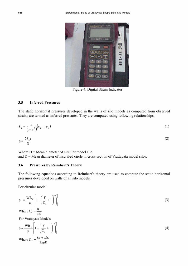
588 Experimental Study of Vrattayata Shape Steel Silo Models
Figure 4. Digital Strain Indicator
3.5 Inferred Pressures The static horizontal pressures developed in the walls of silo models as computed from observed strains are termed as inferred pressures. They are computed using following relationships.
( )( ) 1
ES yx2x νεεν
+−
= (1)
Dt2Sp
x= (2)
Where D = Mean diameter of circular model silo and D = Mean diameter of inscribed circle in cross-section of Vrattayata model silos. 3.6 Pressures by Reimbert’s Theory The following equations according to Reimbert’s theory are used to compute the static horizontal pressures developed on walls of all silo models. For circular model
⎥⎥⎦
⎤
⎢⎢⎣
⎡⎟⎟⎠
⎞⎜⎜⎝
⎛+−=
−2
c
c 1C
1μ
WRp Y (3)
μKRCWhere c
c =
μK2x)r(CWhere
1C
1μ
WRp
ModelsVrattayataFor
vv
2v
ππ
ν
+=
⎥⎥⎦
⎤
⎢⎢⎣
⎡⎟⎟⎠
⎞⎜⎜⎝
⎛+−=
−Y (4)

N.V. Deshpande and L.M. Gupta 589
3.7 Euro Code The expressions for computing the horizontal pressure exerted on vertical walls of silo under fully filled condition as per Euro Code 1 part 4 are as follows :
⎥⎥⎦
⎤
⎢⎢⎣
⎡−=
−R
Ykμ
e1μ
WRp (5)
The code also suggests that for computing p, μ = 0.9 μm and k = 1.15 Km. The value of Km is considered as 1.1 ( 1 - sinφ ). 4. RESULTS The strains recorded during conduction of experiments on all Silo models are used to determine inferred horizontal pressures on walls at predetermined positions of strain-gauges. The horizontal pressures at strain-gauge positions are computed using Reimbert’s theory and by applying Euro code method. The comparison is shown in Table 8 and 9 for models C, V12, V22, V32.
Table 8. Comparison of p for Model ‘C’ & ‘V12’
FOR C FOR V12 p (kN/m2) p (kN/m2) Sl.
No. Y
(m) EURO Reim MC EURO Reim MC MS
1 0.20 1.305 1.071 1.35 1.304 1.066 1.1 0
2 0.35 2.047 1.615 2.7 2.044 1.608 1.76 *
3 0.50 2.632 2.02 3.08 2.682 2.011 2.21 2.06
4 0.65 3.094 2.33 3.74 3.089 2.32 2.99 2.67
5 0.80 3.459 2.57 2.93 3.45 2.562 2.92 3.12
MC indicates inferred pressures on curved wall and MS indicates inferred pressures on straight wall.
Table 9. Comparison of p for Model ‘V22’ & ‘V32’ FOR V22 FOR V32
p (kN/m2) p (kN/m2) Sl. No. Y (m) EURO Reim MC MS EURO Reim MC MS 1 0.20 1.304 1.066 1.107 0.9 1.305 1.066 1.43 1.68 2 0.35 2.045 1.608 2.214 * 2.047 1.609 2.206 2.53 3 0.50 2.683 2.013 2.995 2.54 2.632 2.014 2.86 * 4 0.65 3.091 2.322 3.44 3.44 3.094 2.324 3.31 * 5 0.80 3.455 2.564 2.79 3.24 3.459 2.566 3.1 3.1
Figures 5 to 8 show variation of static horizontal pressures along depth of vertical wall of model C, V12, V22, V32 respectively.

590 Experimental Study of Vrattayata Shape Steel Silo Models
0
0.5 1
1.5 2
2.5 3
3.5 4
0 0.2 0.4 0.6 0.8 1
Depth From Top
Stat
ic H
oriz
onta
l Pre
ssur
e
EURO Reim MC
Figure 5. Variation of Horizontal Pressure Model - C
0
0.5
1
1.5
2
2.5
3
3.5
4
0 0.2 0.4 0.6 0.8 1
Depth From Top
EUROReimMCMS
Figure 6. Variation of Horizontal Pressure Model – V12
0
0.51
1.52
2.5
33.5
4
0 0.2 0.4 0.6 0.8 1
Depth From Top
EUROReimMCMS
Figure 7. Variation of Static Horizontal Pressure Model – V22
00.5
11.5
22.5
33.5
4
0 0.2 0.4 0.6 0.8 1
Depth From Top
Stat
ic H
ori.
Pres
sure
EURO Reim MC MS
Figure 8. Variation of Static Horizontal Pressure Model – V32
(m)
(kN
/m2 )
(m)
(kN
/m2 )
(m)
Stat
ic H
ori.
Pres
sure
(kN
/m2 )
Stat
ic H
ori.
Pres
sure
(kN
/m2 )
(m)

N.V. Deshpande and L.M. Gupta 591
5. DISCUSSION • The ratio of length of straight portion to radius of semicircular portion in Vrattayata shape
models is selected as 0.2 so that some feasible dimension from fabrication point of view is possible.
• The internal volume enclosed within vertical walls of all silo models is kept unchanged so that the same quantity of material in all models can be filled.
• Moisture free dry sand is used as stored material as dampness in sand affects its characteristics.
• The thickness of sheet used in model silos being very small, it is susceptible for melting in arc welding. Hence, spot welding is used with specific current rating.
• The principal characteristics (W, φ, δ) of stored material are determined in the laboratory to have their appropriate values rather than selecting them from standard books or codes.
• The static horizontal pressures on walls of model silos are computed using two dimensional stress–strain relationship in which measured horizontal and vertical strains are assumed to be principal strains.
• The static horizontal pressures computed from measured strains on wall of Model C and curved walls of Model V12, V22, V32 show similar trend as obtained by Euro Code Method and Reimbert’s theory. But the curve is closer to curve as obtained by Euro Code Method than Reimbert’s theory. Generally, these pressures on curved surfaces are more than those predicted by Reimbert’s theory predictions at corresponding depths.
• The assumption that the inferred pressures at a particular depth would be the same at curved wall and at straight wall of Vrattayata models does not appear to be correct as differences are seen between the inferred pressures at a particular depth on curved wall and on straight wall. In the models V22, V32, the trend observed for inferred pressures on straight wall is the same as that for curved wall. But in the Model V12, such trend is seen only in lower half of the wall. This may be due to disturbances in stresses caused at the joints between the straight wall and curved wall and the development of small magnitude bending stresses. The trend of increase in inferred pressures along the depth of straight wall is seen generally in most of the models. These curves are closer to curves predicted by Euro Code Method than by Reimbert’s theory.
• The main reasons for observed differences at many points are as follows. o Material used for wall does not possess the same properties everywhere. o Creation of imperfections in model walls during process of fabrication. o The stiffener plates provided at top and bottom of model walls affect the strains. Such plates
are not envisaged from the predictions by Euro Code Method and Reimbert’s theory. o The bulk density of sand, which is used as stored material, varies along the depth.
• The ratio of lateral pressure to vertical pressure actually varies along the depth of silo wall. This variation of pressure ratio is appropriately considered in Reimbert’s theory by considering suitably the characteristic abscissa in its formulation.
• When static horizontal pressures are calculated following guidelines of Euro code 1 part 4 (1996) for all four models at 0.5 m depth, it is observed that the variation between these pressures and corresponding inferred pressures is not more than 27%.

592 Experimental Study of Vrattayata Shape Steel Silo Models
6. CONCLUSIONS 1. For Vrattayata shape, three dimensions, its radius of semi-circular portion, its length of straight
portion and its height can decide its volume content, but in circular shape only two dimensions, its radius and height can decide its volume content.
2. Reimbert’s theory for silo takes into account the effect of shape by considering the characteristic abscissa in predicting the wall pressures.
3. Slight imperfection in silo geometry causes increase in pressure. 4. The measured strains in a particular vrattayata silo model at the same depth are not the same on
curved walls and straight walls. REFERENCES [1] Lenczner, D., “An Investigation into the Behavior of Sand in a Model Silo”, The Structural
Engineer, December 1963, Vol. 41, pp. 389 – 398. [2] Garg, R.M. and Gopalkrishnan, S., “An Experimental Investigation of Wall Loads in Wheat
Silos”, Indian Concrete Journal, October 1974, pp. 308–313. [3] Blight, G.E., “Pressures Exerted by Materials Stored in Silos : Part I, Coarse Materials”,
Journal of Geotechnique, Vol. 36, No. 1, 1986, pp. 33–46. [4] Blight, G.E., “Pressures Exerted by Materials Stored in Silos : Part II, Fine Powders”,
Journal of Geotechnique, Vol. 36, No. 1, 1986, pp. 47 – 56. [5] Eurocode 1 : DD ENV 1991 – 4 : 1996, “Basis of Design and Actions on Structures”, Part 4.
Actions in Silos and Tanks, British Standards Institutions. [6] Reimbert, M.L. and Reimbert, A.M., “Silos Theory and Practice”, Trans Tech Publications,
1976, Vol. 1, No. 3. [7] Safarian, S.S., Harris, E.C., “Design and Construction of Silos and Bunkers”, Publishers
Van Nostrand Reinhold Company, New York, U.S.A., 1985.

N.V. Deshpande and L.M. Gupta 593
NOTATIONS A Area of horizontal cross–section through silo (m2) Ac, Av Area of horizontal cross – section through circular and Vrattayata silos respectively. (m2) Cc, Cv Reimbert’s characteristic abscissa for circular and Vrattayata silos respectively E Modulus of Elasticity (kN/m2) H Height of vertical wall of silo (m) Hc, Hv Height of vertical wall for circular and Vrattayata silos respectively (m) L Length of Straight portion of the wall of Vrattayata silo (m) R Hydraulic Radius ( A / U ) (m) Rc, Rv The hydraulic radius for circular and Vrattayata shape silos respectively (m) Sx Stress in X direction (kN/m2) U Perimeter of horizontal cross – section (m) Uc, Uv Perimeter of horizontal cross – section of circular and Vrattayata silos respectively (m) V Internal volume of container enclosed by vertical wall of silo (m3) W Bulk Density of stored material (kN/m3) Y Depth of stored material above the point in question (m) k Ratio of horizontal to vertical pressure by stored material Km Mean value of ratio of horizontal to vertical pressure by stored material p Static horizontal pressure on silo walls due to stored material (kN/m2) rc Internal radius of circular silo (m) rv Internal radius of semi - circular portion of Vrattayata silo (m) t Thickness of wall (mm) x The ratio of length of straight portion to radius of semi – circular portion of Vrattayata silo
(L/rv) μ The coefficient of wall friction ( tan δ ) μm Mean coefficient of wall friction φ The angle of internal friction of stored material δ The angle of wall friction ν Poisson's ratio for wall material εx, εy Measured strains in X and Y directions respectively

Advanced Steel Construction Vol. 3, No. 2, pp. 594-606 (2007) 594
DESIGNING COMPOSITE BEAMS WITH PRECAST HOLLOWCORE SLABS TO EUROCODE 4
D. Lam
Senior Lecturer, School of Civil Engineering, University of Leeds, Leeds, LS29JT, UK
(Corresponding author: E-mail: [email protected])
Received: 15 November 2005; Revised: 26 January 2007; Accepted: 1 February 2007
ABSTRACT: The design of multi-storey buildings in the UK, in the past, considered steel and concrete structures in isolation. Today, designers utilize the combined properties of steel and concrete in the form of composite or hybrid structures as a more attractive efficient alternative. Designers of steel structures acknowledge that the presence of concrete slabs may be designed compositely with steel beams in order to increase both flexural strength and stiffness at virtually no extra cost, except for the headed shear studs. The use of composite construction with precast hollowcore slabs has become one of the most popular construction methods in the UK. Currently, design of composite construction is covered by BS5950, Part 3, but will soon be replaced by the new European Standard, Eurocode 4. However, design of composite construction with precast hollowcore slabs is currently outside the provisions of this new code. In this paper, an overview of the Eurocode 4 structure and its contents are first presented and some of the particular issues that affect this new form of construction will be given. Design guidance using the Eurocode methodology will also be presented.
Keywords: Eurocode 4; composite design; precast; hollowcore; steel; connection design; moment capacity; effective length
1. INTRODUCTION The environmental impacts of human activities have risen to the forefront of international concern in recent years. A mixture of legislation, public opinion and social responsibility has driven construction industries throughout the world to reduce pollution and waste. Among all sectors of economic activity, the buildings and construction sector has by far the greatest environmental impact in terms of resource consumption and offers enormous scope for improvement. As the construction industry demands for rapid construction with reduction in cost and environmental impacts, composite construction, especially those without major onsite concreting, has become very popular among the designers and engineers in the UK. Use of composite elements in the form of beams, and slabs are already common in the UK. The application is currently supported by the British Standard, BS5950, Part 3 [1] but will soon be replaced by a new standard harmonized across Europe, EN1994 – Eurocode 4 [2]. This code formed part of a complete set of design codes developed in the Eurocode programme by the European Standards Organization (CEN) initiated by the Commission of the European Communities. The programme aims to harmonize all the code of practices across the whole European communities, it also aims to harmonize between different construction materials, e.g. steel, concrete, masonry etc, and construction methods to achieve full consistency and compatibility in terms of loading, safety factors so that a comparable safety levels can be obtained. In 1975, the Commission of the European Community decided on an action programme in the field of construction, based on article 95 of the Treaty. The objective of the programme was the elimination of technical obstacles to trade and the harmonization of technical specifications. Within the programme, the Commission took the initiative to establish a set of harmonized technical rules for the design of construction works which, in a first stage, would serve as an alternative to the national rules in force in the Member States and, ultimately, would replace them.

595 D. Lam
The National Standards implementing Eurocodes will comprise the full text of the Eurocode (including any annexes), as published by CEN, which may be preceded by a National title page and National foreword, and may be followed by a National annex. The National annex may only contain information on those parameters, which are left open in the Eurocode for national choice, known as Nationally Determined Parameters, to be used for the design of buildings and civil engineering works to be constructed in the country concerned, i.e.: - values and/or classes where alternatives are given in the Eurocode, - values to be used where a symbol only is given in the Eurocode, - country specific data (geographical, climatic, etc.), e.g. snow map, - the procedure to be used where alternative procedures are given in the Eurocode. It may also contain - decisions on the use of informative annexes, and - references to non-contradictory complementary information to assist the user to apply the
Eurocode. 1.1 Eurocode 4 – EN1994 Eurocode 4 was first drafted in 1985 and published in 1992 as ENV1994 and accompanied by the National Application Documents (NAD’s). It is intended that the Eurocode together with its NAD may be used optional to the National Standard. The difficulty associated with the Eurocode 4 document is that the code must be consistent on one hand with the material independent parts of EN1990 [3] & EN1991 [4] and on the other hand, consistent with the Eurocode 2 [5] for concrete structures and Eurocode 3 [6] for the steel structures. For this consistency, CEN insisted that information is not repeated in each code but referring across the codes. Therefore, EN1994 must be used in conjunction with all the related Eurocodes. For this reason, it is difficult to design using the Eurocode 4 until all the other Eurocodes are ready. Figure 1 shows the relationship of the EN1994 with the other Eurocodes.
Figure 1. Designing Composite Structures Using the Eurocodes
EN1994 Composite Structures
EN1993 Steel
Structures
EN1992 Concrete
Structures
EN1991 Actions
Dead Imposed Wind
EN1990 Basis of Design

Designing Composite Beams with Precast Hollowcore Slabs to Eurocode 4 596
As shown in Figure 1, for the design of the composite structures, material properties related to concrete part of the structures must be referred to the EN1992, i.e. grade, modulus of elasticity and strength of the concrete, while the material properties related to the steel part of the composite structures must be referred to the EN1993, for example, steel grade, yield strength and modulus of elasticity. In addition, design rules such as effective width, classification of cross sections, etc. will need to be consistent across all the related codes. Part 1-1 of Eurocode 4 gives a general basis for the design of composite structures together with specific rules for buildings. The following subjects are dealt with in Part 1-1: Section 1: General Section 2: Basis of design Section 3: Materials Section 4: Durability Section 5: Structural analysis Section 6: Ultimate limit states Section 7: Serviceability limit states Section 8: Composite joints in frames for buildings Section 9: Composite slabs with profiled steel sheeting for buildings Annex A: Stiffness of joint components in buildings. Annex B: Standard tests. Annex C: Shrinkage of concrete for composite structures for buildings. As discussed earlier on, composite construction with precast hollowcore slabs is currently outside the provisions of the current EN1994. This paper discusses some of the particular issues that affect this form of construction, and presents a design guidance using the Eurocode methodology. 2. COMPOSITE CONSTRUCTION WITH PRECAST HOLLOWCORE SLABS In composite construction, the most important piece of information relevant to composite beam design is the shear connectors load – slip capacity. This load-slip characteristic of the shear connectors have mainly been obtained from the push off tests. Although the push off test cannot exactly simulate the actual conditions occurring in a composite beam, it does enable the behaviour of different types and sizes of shear connectors to be compared provided the test is standardized. The standard push off test for shear connectors is currently covered by Annex B in the EN1994-1-1and as shown in Figure 2. 2.1 A. Basis of Design for the Shear Connectors The basis principles for the design of shear connector are as follow: (1) Shear connectors and transverse reinforcement shall be provided to transmit the longitudinal
shear force between the concrete and the structural steel element, ignoring the effect of natural bond between the two.
(2) Shear connectors shall have sufficient deformation capacity to justify any inelastic redistribution of shear assumed in design.
(3) Ductile connectors are those with sufficient deformation capacity to justify the assumption of ideal plastic behaviour of the shear connection in the structure considered.
(4) A connector may be taken as ductile if the characteristic slip capacity δuk is at least 6mm. An evaluation of δuk is given in Annex B of the EN1994-1-1.
(5) Shear connectors shall be capable of preventing separation of the concrete element from the steel element, except where separation is prevented by other means.

597 D. Lam
(6) To prevent separation of the slab, shear connectors should be designed to resist a nominal ultimate tensile force, perpendicular to the plane of the steel flange, of at least 0.1 times the design ultimate shear resistance of the connectors. If found necessary, they should be supplemented by anchoring devices.
(7) Headed stud shear connectors may be assumed to provide sufficient resistance to uplift, unless the shear connection is subjected to direct tension.
(8) Longitudinal shear failure and splitting of the concrete slab due to concentrated forces applied by the connectors shall be prevented.
As the current standard push off test is not suitable for composite precast hollowcore construction, a new standardize push off test is needed to fill the gap in the Eurocode 4. Key 1 Cover 15 mm 2 Bedded in mortar or gypsum 3 Recess optional 4 Reinforcement: ribbed bars φ10 mm resulting in a high bond with 450 ≤ fsk ≤ 550 N/mm2 Steel section: HE 260B or 254 × 254 × 89 kg/m UC
Figure 2. Test Specimen for Standard Push Off Test
2.1.1 New push off test for hollowcore slabs A new horizontal push off test arrangement is proposed by Lam [7] as shown in Figure 3. The test specimens each consisted of four 600mm wide x 800mm long prestressed hollowcore units connected to a 254 x 254 x 73 UC with a single row of 6 pre-welded headed studs at 150mm centres. Cores of 500mm long were left open to allow placement of the transverse reinforcement.
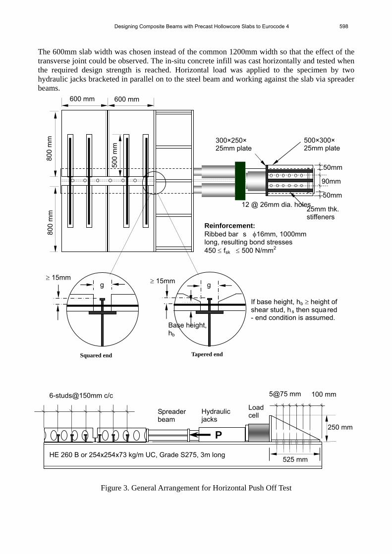
Designing Composite Beams with Precast Hollowcore Slabs to Eurocode 4 598
The 600mm slab width was chosen instead of the common 1200mm width so that the effect of the transverse joint could be observed. The in-situ concrete infill was cast horizontally and tested when the required design strength is reached. Horizontal load was applied to the specimen by two hydraulic jacks bracketed in parallel on to the steel beam and working against the slab via spreader beams.
Figure 3. General Arrangement for Horizontal Push Off Test
50mm
50mm
90mm
12 @ 26mm dia. holes
500×300× 25mm plate
300×250× 25mm plate
25mm thk. stiffeners
Reinforcement: Ribbed bar s φ16mm, 1000mm long, resulting bond stresses 450 ≤ fsk ≤ 500 N/mm2
Squared end
≥ 15mm
800
mm
80
0 m
m
Base height, hb
If base height, hb ≥ height of shear stud, h s then squared - end condition is assumed.
Tapered end
≥ 15mm
500
mm
g g
600 mm 600 mm
6-studs@150mm c/c 5@75 mm 100 mm
HE 260 B or 254x254x73 kg/m UC, Grade S275, 3m long
Spreader beam
Hydraulic jacks
Load cell
525 mm
P 250 mm
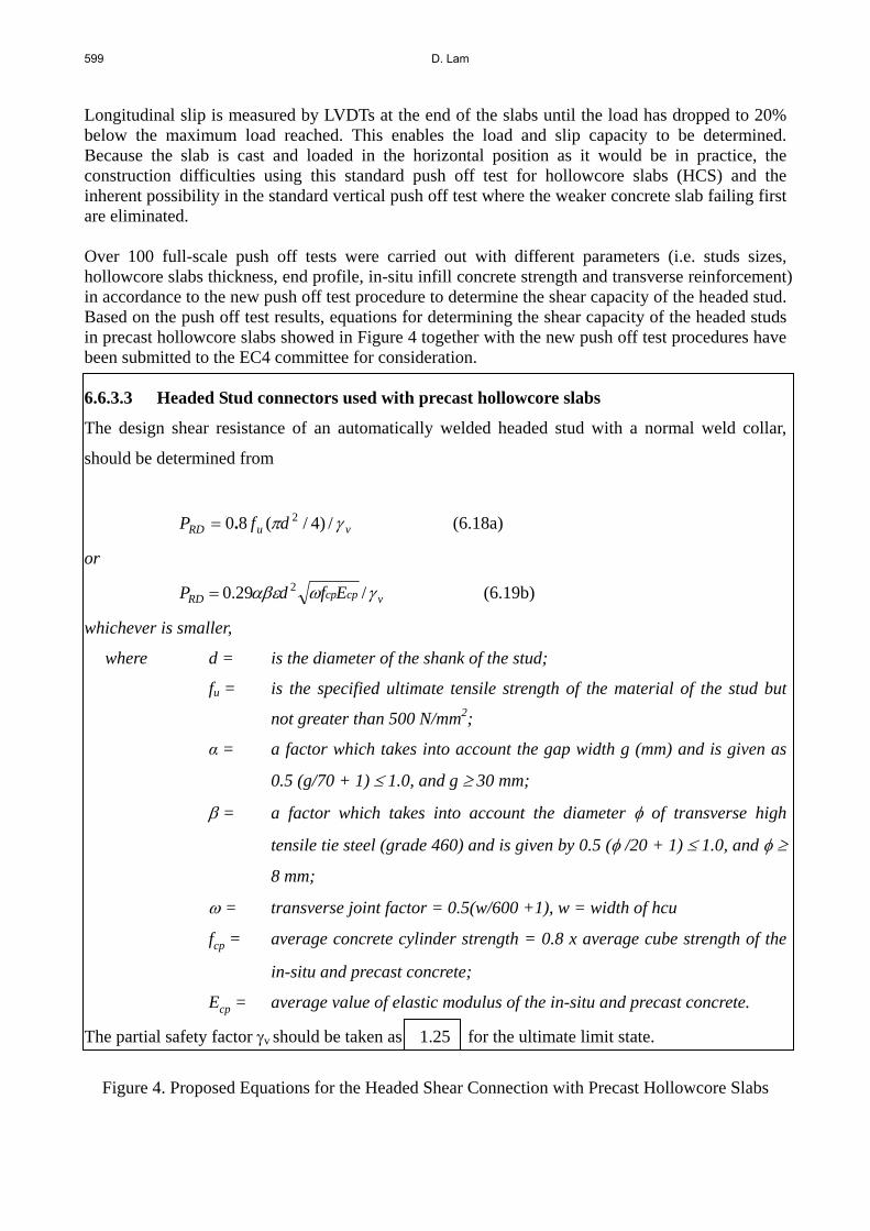
599 D. Lam
Longitudinal slip is measured by LVDTs at the end of the slabs until the load has dropped to 20% below the maximum load reached. This enables the load and slip capacity to be determined. Because the slab is cast and loaded in the horizontal position as it would be in practice, the construction difficulties using this standard push off test for hollowcore slabs (HCS) and the inherent possibility in the standard vertical push off test where the weaker concrete slab failing first are eliminated. Over 100 full-scale push off tests were carried out with different parameters (i.e. studs sizes, hollowcore slabs thickness, end profile, in-situ infill concrete strength and transverse reinforcement) in accordance to the new push off test procedure to determine the shear capacity of the headed stud. Based on the push off test results, equations for determining the shear capacity of the headed studs in precast hollowcore slabs showed in Figure 4 together with the new push off test procedures have been submitted to the EC4 committee for consideration. 6.6.3.3 Headed Stud connectors used with precast hollowcore slabs
The design shear resistance of an automatically welded headed stud with a normal weld collar,
should be determined from
vuRD dfP γπ /)4/(80 2.= (6.18a)
or
vcpcpRD EfdP γωαβε /29.0 2= (6.19b)
whichever is smaller,
where d = is the diameter of the shank of the stud;
fu = is the specified ultimate tensile strength of the material of the stud but
not greater than 500 N/mm2;
α = a factor which takes into account the gap width g (mm) and is given as
0.5 (g/70 + 1) ≤ 1.0, and g ≥ 30 mm;
β = a factor which takes into account the diameter φ of transverse high
tensile tie steel (grade 460) and is given by 0.5 (φ /20 + 1) ≤ 1.0, and φ ≥
8 mm;
ω = transverse joint factor = 0.5(w/600 +1), w = width of hcu
fcp = average concrete cylinder strength = 0.8 x average cube strength of the
in-situ and precast concrete;
Ecp = average value of elastic modulus of the in-situ and precast concrete.
The partial safety factor γv should be taken as 1.25 for the ultimate limit state.
Figure 4. Proposed Equations for the Headed Shear Connection with Precast Hollowcore Slabs

Designing Composite Beams with Precast Hollowcore Slabs to Eurocode 4 600
2.1.2 Effective width of flanges for shear lag In composite design, allowance need to be made for the flexibility of the concrete flanges affected by in-plane shear (shear lag), it can be done either by means of rigorous analysis, or by using an effective width of the concrete flange. In EC4, the effective width of concrete flanges is determined in accordance with Figure 5. When elastic global analysis is used, a constant effective width may be assumed over the whole of each span. This value may be taken as the value beff,1 at mid-span for a span supported at both ends, or the value beff,2 at the support for a cantilever. At mid-span or an internal support, the total effective width beff, see Figure 5, may be determined as:
beff = b0 + ∑bei (1)
where: b0 is the distance between the centres of the outstand shear connectors; bei is the value of the effective width of the concrete flange on each side of the web and taken
as Le/8 but not greater than the geometric width bi . The value bi should be taken as the distance from the outstand shear connector to a point mid-way between adjacent webs, measured at mid-depth of the concrete flange, except that at a free edge bi is the distance to the free edge.
The effective width at an end support may be determined as:
beff = b0 + ∑ βi bei (2)
with
βi = (0,55 + 0,025 Le / bei) ≤ 1,0 (3)
where: bei is the effective width of the end span at mid-span and Le is the equivalent span of the end
span according to Figure 5. 2.1.3 Effective width of hollowcore slabs The calculation for the effective width of the hollowcore slabs is more complicated than the Eurocode method due to the presence of the hollow cores (voids) within the concrete slabs. Figure 6 shows the section of the composite beam with precast hollowcore slabs. From the results of the experimental work and FE analyses carried out by Lam et al. [8, 9] and Murad & Lam [10], it showed that the effective width for this form of construction is affected by the in-situ concrete infill, the precast hollowcore slabs and the transverse reinforcement. Based on the research work, an empirical equation for calculating effective width for the hollowcore slabs is proposed:
gff
b sdrickeff 5.21000
46050032
35, +×××=
φ (4)

601 D. Lam
Figure 5. Equivalent Spans for Effective Width of Concrete Flange
where fck,i is the in-situ infill concrete strength in N/mm2. φr is the diameter of the transverse reinforcement in mm. fsd is the characteristic strength of the transverse reinforcement in N/mm2. g is the gap between the precast units
Figure 6. Effective Width of Hollowcore Slabs
beff

Designing Composite Beams with Precast Hollowcore Slabs to Eurocode 4 602
2.2 Moment Resistance of the Composite Beams The bending resistance of the composite beams can be determined by rigid-plastic theory only where the effective composite cross-section is in Class 1 or Class 2. Otherwise, elastic analysis and non-linear theory for bending resistance may be applied to cross-sections of any class. It is assumed that the composite cross-section remains plane if the shear connection and the transverse reinforcement are designed in accordance with Cl.6.6, to distribute the design longitudinal shear force. The tensile strength of concrete shall be neglected. The following assumptions should be made in the calculation of Mpl,Rd : a) there is full interaction between structural steel, reinforcement, and concrete; b) the effective area of the structural steel member is stressed to its design yield strength fyd in
tension or compression; c) the effective areas of longitudinal reinforcement in tension and in compression are stressed to
their design yield strength fsd in tension or compression. Alternatively, reinforcement in compression in a concrete slab may be neglected;
d) the effective area of concrete in compression resists a stress of 0.85fcd constant over the whole depth between the plastic neutral axis and the most compressed fibre of the concrete, where fcd is the design cylinder compressive strength of concrete.
Typical plastic stress distributions are shown in Figure 7.
Figure 7. Plastic Stress Distributions under Sagging Bending for Partial Shear Connection
2.2.1 Moment resistance of composite beams with precast hollowcore slabs For composite beams with precast hollowcore slabs, similar rigid plastic theory is applied. The only limitation applied for this form of construction is that the plastic neutral axis is below the steel – concrete interface. Figure 8 shows the plastic stress distributions under sagging bending with full shear connection.

603 D. Lam
Figure 8. Plastic Stress Distributions under Sagging Bending for Full Shear Connection
The moment resistance of the composite sections where neutral axis is within the web is given below:
⎟⎟⎠
⎞⎜⎜⎝
⎛−
++=
wa
fcslabfcaplRdpl N
NDDDNMM
,
2,
,,, 42)(
(5)
where Mpl,a is the moment resistance of the steel section D is the steel section depth Dslab is the concrete slab depth Nc,f is the compressive resistance of the concrete flange Na,w is the resistance of the web of the steel section 2.3 D. Composite Joints In steel braced frame structures, the most economical solution is to use nominal pinned joints. However, since longitudinal reinforcement is required over the supports; in order to limit cracking in providing additional tying against disproportional collapse, it will be technically and economically advantages to design the joints as composite joints in which the longitudinal reinforcement will contribute to the resistance and the stiffness of the joint. Composite joints in building are covered in section 8 of Eurocode 4 and the section is consistent with the EN1993-1-8 [11]. The design of moment capacity of these joints are based on the so-called ‘component method’. Figure 9 shows the example of the composite joints. With regard to the rotation capacity of these joints, the influence of cracking of concrete, tension stiffening and deformation of the shear connection should be considered in determining the rotation capacity. The rotation capacity of a composite joint may be demonstrated by experimental evidence. Alternatively, calculation methods may be used, provided that they are supported by tests. In general, composite joints with rotation capacity in excess of 30 mRad are acceptable for design purposes.
0.85 fcd × beff × Dslab
fyd
fyd

Designing Composite Beams with Precast Hollowcore Slabs to Eurocode 4 604
Figure 9. Composite Joint
2.3.1 Composite joints with precast hollowcore slabs Figure 10 shows the force diagram and component of the composite joints. Equation (6) based on the component method are proposed to predict the rotation capacity, φu for this form of composite joints. From the strain profile of the longitudinal reinforcing bar taken from the tests data by Lam & Fu [12], it shows that the steel bar yielded only in the region between the column centre line and the second shear stud, the strain in the other part of the steel bar is small and remained elastic. Therefore, the elongation zone of the longitudinal reinforcement, ΔL can be taken as between the centre line of the column and the position of the second stud. Hence, it can assumed that the length for calculating the elongation to be p1+p2+D/2, where p1 is the distance between the column face and the centre line of the first stud; p2 is the distance between the centre line of the first stud and the second stud and D is the depth of the column.
Figure 10. Force Diagram and the Components of the Composite Joint
p1 p2
ΔL
Dr
Db
r1 Fb,t
Na,f
Fr,t
D

605 D. Lam
brbu D
SlipDD
L+
+=
Δφ (6)
where )2
( 21DppL sh ++= εΔ
For full shear connection, reinforcement strain, εsh is taken as the ultimate strain developed in the longitudinal reinforcement. It is because that for full shear connection, the longitudinal reinforcing bars can be developed into the strain hardening whereas for the partial shear connection, εsh is taken as the maximum strain developed in the longitudinal bar. For simplicity, it can be taken as the yield strain of the steel bars if enough shear studs are provided to enable yielding of the longitudinal bars. The moment resistance of the composite joint, MRd For trtbfa FFN ,,, +≥ where, Na,f = compressive resistance of the bottom flange of the steel beam, Fr,t = tensile strength of the longitudinal reinforcement, Fb,t= effective tensile resistance of the bolt group.
)5.0()5.0( 1,, fbtbfrbtrRd trDFtDDFM −−+−+= (7) where, Db = the depth of the beam, r1 = the distance of the first row of bolts below the top of the beam, Dr = the distance of the reinforcement above the top of the beam, tf = the flange thickness of the steel beam. For trtbfa FFN ,,, +< ,
The neutral axis, ydw
fatbtrc ft
NFFy
)( ,,, −+=
where, tw = the web thickness and fyd = the design strength of steel section. The moment resistance of the composite connection, MRD
2)5.0()5.0( ,1,,
ctwfbtbfrbtrRD
yFtrDFtDDFM −−−+−+= (8)
where ydwcw ftyR = 3. CONCLUSIONS In this paper, an overview of the Eurocode structures and the contents of the Eurocode for composite construction, EN1994 are presented. In particular, technical details especially related to the design of the composite beams are discussed and compared with the treatment to the composite construction with precast hollowcore slabs. Design guidance for this form of construction using the

Designing Composite Beams with Precast Hollowcore Slabs to Eurocode 4 606
Eurocode methodology is discussed and new equations and design method are proposed. ACKNOWLEDGEMENT The author would like to acknowledge the financial support from the International Precast Hollowcore Association (IPHA) and Overseas Research Scholarship (ORS), the support provided by Severfield – Revee Structures Ltd. for supplying the steel specimens and Bison Concrete Products Ltd. for supplying the precast hollowcore slabs. The skilled assistance provided by the technical staff in the School of Civil Engineering at University of Leeds is also appreciated. REFERENCES [1] BS5950, Part 3, Structural Use of Steelwork in Building – Design in Composite
Construction, British Standards Institution, London, 1990. [2] EN1994-1-1, Eurocode 4: Design of Composite Steel and Concrete Structures: Part 1.1:
General rules and rules for buildings, British Standards Institution, London, 2004. [3] EN1990, Eurocode – Basis of Structural Design, British Standards Institution, London,
2002. [4] EN1991, Eurocode 1 – Actions on Structures, British Standards Institution, London, 2002. [5] EN1992-1-1, Eurocode 2 – Design of Concrete Structures, British Standards Institution,
London, 2004. [6] EN1993-1-1, Eurocode 3 – Design of Steel Structures, British Standards Institution, London,
2005. [7] Lam, D., “New Test for Shear Connectors in Composite Construction”, United Engineering
Foundation Conference, Composite Construction in Steel and Concrete IV, Banff, Alberta, Canada, 2000, pp. 404-414.
[8] Lam, D., Elliott, K.S. and Nethercot, D.A., “Experiments on Composite Steel Beams with Precast Concrete Hollow Core Floor Slabs”, Proceedings of the Institution of Civil Engineers: Structures and Buildings, 2000a, Vol. 140, pp. 127-138.
[9] Lam, D., Elliott, K.S. and Nethercot, D.A., “Parametric Study on Composite Steel Beams with Precast Concrete Hollow Core Floor Slabs”, Journal of Constructional Steel Research, 2000b, Vol. 54, No. 2, pp. 283-304.
[10] Murad, A. and Lam, D., “Experimental Study of Long Span Composite Beams with Precast Hollow-Core Slabs”, Eurosteel, 4th European Conference on Steel and Composite Construction, Maastricht, 2005.
[11] EN1993-1-8, Eurocode 3 – Design of Steel Structures, Part 8: Design of Joints, British Standards Institution, London, 2005.
[12] Lam, D and Fu, F., “Behaviour of Composite Steel Beams with Precast Hollow Core Slabs in Hogging Moment Regions”, 4th International Conference on Advances in Steel Structures, Shanghai, China, 2005.

Advanced Steel Construction Vol. 3, No. 2, pp. 607-627 (2007) 607
EXPERIMENTAL AND THEORETICAL INVESTIGATIONS OF PALLET RACKS CONNECTIONS
Lucjan Ślęczka and Aleksander Kozłowski
Rzeszów University of Technology, Department of Building Structures, W. Pola 2, 35-959 Rzeszów, Poland
Fax.: +48-17-8542974 (Corresponding author: E-mail: [email protected])
Received: 16 November 2006; Revised: 24 January 2007; Accepted: 5 February 2007
ABSTRACT: Steel storage pallet racks are three-dimensional framed structures, similar to multi-storey building structures. They are widely used for the storage of different types of materials. To provide the easy accessibility to stored products, pallet racks are not braced in down-aisle direction. The only source of the stiffness required for down-aisle stability is the stiffness of the connections between columns and beams, and the stiffness of the column bases. Connections between columns and beams are realized by means of different types of mechanical devices (tabs, hooks etc) without the need of using bolts and welds. Such joints have non-linear φ−M characteristic. Most of the recent design codes and papers recommend experimental tests of beam-to-column connections to obtain semi-rigid joint characteristics that can be applied in the global analysis. The aim of this paper is to present application of the component method to assess main joint properties, i.e. the moment resistance and initial stiffness of storage rack joints. Results obtained using developed model are compared with the test results.
Keywords: Storage pallet racks, component method, semi-rigid connection, experimental tests
1. INTRODUCTION Steel pallet racks are regular, 3D multi-storey, multi-bay structures, used in industry and warehouses for the storage of palletised goods (Fig. 1). They are realized by using cold-formed steel profiles. Design analysis of such structures is carried out on 2D sub-assemblies, separately in the cross- and down-aisle directions. Stability in the cross-aisle direction is provided by bracings. To provide the easy accessibility to stored products, pallet racks are not braced in down-aisle direction. Because of lack of bracings in the down-aisle direction, structural analysis is carried out by adopting a semi-continuous sway frame model, i.e. unbraced frame with semi-rigid joints. Analysis of such structures were described in a few papers (Abdel-Jaber et al [1], Beale and Godley [2], Bernuzzi and Castiglioni [3], Freitas et al [4], Godley et al. [5], Peköz and Rao [6], The et al. [7]) Connections between columns and beams are realized in such structures by means of different types of mechanical devices such tabs, hooks etc, without the need of using bolts and welds. These joints have non-linear φ−M characteristic (Baldassino and Zandonini [8], Baldassino and Bernuzzi [9], Markazi et al. [10], Markazi et al. [11]. Most of the recent design codes and papers, recommend an experimental-theoretical design approach and require experimental tests of beam-to-column connections to obtain semi-rigid joint characteristics that can be applied in the global analysis. Such experimental tests were conducted for one of the commercially available steel racks system in Poland. Observation of joint behaviour during tests suggests the possibility of using the component method to evaluate the main joint properties i.e. moment resistance and initial stiffness. The aims of the paper are to present model of the component method for the investigated rack joints and compare results between the tests and the component modelling.

608 Ex perimental and Theoretical Investigations of Pallet Racks Connections
Figure 1. Typical Pallet Racks Configuration
2. EXPERIMENTAL PROCEDURE AND THE TEST RESULTS A sketch of tested beam-to-column connection with its dimensions is shown in Figure 2. The joint consists of a beam-end connector with tabs, made of a 4-mm thick cold-formed angle, welded to each end of the beam. The leg of the angle with tabs is in contact with column web after assembly, while there is a 2-mm gap between the second leg, perpendicular to the column web.
A
Beam-end- connector
RHS Beam
Column
Slots
A-A2 mm gap
90
75
2
Cantilevered tabs
250
Beam-end-connector
A
RHS Beam
4
37
19
50
4 x
50
After the assembly
Before the assembly
Figure 2. Dimensions of Tested Joint

Lucjan Ślęczka and Aleksander Kozłowski 609
Recommendations (Institute of Logistics and Warehousing [12]) suggest two possible ways of testing to evaluate the joint behaviour. One is bending test on isolated beam-column connection, second is portal test, where the frame, composed of two columns and one beam, is loaded by vertical and horizontal forces. Bending tests on isolated connections were conducted for analysed connections. Research program is summarized in Table 1. The main aim of experimental tests was to obtain moment-rotation characteristics of tested joints and also the observation of behaviour of joint components under loading and finally failure modes. Figure 3 shows the general layout of the tests. Tests were carried out on five full-scale joint groups. Two groups (“D” and “F”) consisted of single-sided joints of external columns. Other three groups (group “B”, “C” and “E”) were double- sided connections of beams to internal columns. Every tested group had the same connector and column section, while the size of the beam was different in each group. To prevent lateral movements whilst loading, both column and beams elements were doubled and connected to each other. Distance 21 ee = was established so, as the force F equal to %25 of shear capacity of connection could produce ultimate bending moment value with tolerance %30± (Institute of Logistics and Warehousing [12]). In order to assess end rotations of the beams, two dial gauges were used at each beam. End rotations of beam were obtained as the relative gauges displacements divided by the separation between them. Because of large stiffness of beam, no correction factor was used for the calculation of the joint rotation (with regard to deflection of the cantilevered beam). In one sided-tests, rotations of the connection was obtained by subtracting the rotation of the column from the rotation of the beam. Testing procedures, instrumentation and detailed test results of analysed joints can be found in (Kozłowski and Ślęczka [13]).
Table 1. Research Program
Symbol Number of specimens Type of tests Type of
beam (RHS) Group “B” 6 Bending tests, internal column 350100 xx Group “C” 6 Bending tests, internal column 34080 xx Group “D” 5 Bending tests, external column 350100 xx Group “E” 6 Bending tests, internal column 360120 xx Group “F” 6 Bending tests, external column 360120 xx
F
e1
Dial gauges
e2
F
Column
Beam-end connector
100 mm
40 mmBeam
e1
F
Column
Beam-end connector
100 mm
40 mm Beam
155 mm
200 mm
Support
Figure 3. General Layout of Double-sided (Internal Column) and
One-sided (External Column) Tests The main test results are summarized in Table 2 and Table 3. Every tested group has consisted of six specimens. Values presented in Tables 2 and 3 are arithmetic mean values. The plastic flexural resistance pexplM , was obtained as a point of intersection of a straight line representing initial

610 Ex perimental and Theoretical Investigations of Pallet Racks Connections
stiffness inijS , , with the line of slope inijS ,1,0 , which is tangent to the non-linear part of the curve obtained in test (Fig. 4).
Table 2. Material Properties Part of the joint Yield stress, [MPa] Ultimate stress, [MPa] Elongation, [%]
Column Connector Beam
384.2 346.6 404.7
431.4 403.3 433.3
30.7 37.2 36.9
Table 3. Main Test Results of Joints
Initial rotational stiffness inijS ,
[kNm/rad]
Plastic flexural resistance exp,plM
[kNm]
Ultimate flexural resistance exp,uM
[kNm] Group “B” Group “C” Group “D” Group “E” Group “F”
139,40 116,70
71,35 123,06
96,15
3,19 2,36 3,10 3,20 3,37
3,90 3,27 3,58 3,73 3,86
0.0
1.0
2.0
3.0
4.0
0 0.02 0.04 0.06 0.08 0.1
φ [rad]
M [kNm]
0.1Sj,ini
experimental
1
Sj,ini
Mpl,exMu,exp
Figure 4. Experimental φ−M Curve, Specimen B5
3. APPLICATION OF COMPONENT METHOD TO MODELLING OF PALLET
RACK CONNECTIONS The component method is now one of the most effective methods to analyze and predict the rotational behaviour of different types and different configurations of connections. It is mainly used in case of steel joints made from hot rolled sections (EN 1993-1-8 [14]) and composite joints (EN 1994-1-1 [15]), but recently has also found other applications (Fink et al. [16]). The application of the component method is usually performed in three stages. The first stage is the identification of components in the analyzed joint, where the complex joint is subdivided into parts. The second stage is the prediction, for each identified component, of its individual initial stiffness, strength and often deformation capacity. The behaviour of each component is described by a bilinear relationship between displacement and force. Components that do not affect the stiffness of the joint are modelled as rigid-plastic, while other components are modelled as elasto-plastic

Lucjan Ślęczka and Aleksander Kozłowski 611
elements. The third stage is the evaluation of flexural strength and rotational stiffness of the whole joint. In this stage, the lever arms should also be predicted for every group of components. Behaviour of connection is then predicted by analysing group of springs with axial stiffness, joined in series or in parallel. 3.1 Identification of Components In the case of analyzed storage rack joint, the following components can be identified: 3.1.1 Column web in tearing A part of the column web situated between the slot and the flange of the column is subjected to a distributed load transmitted by the tabs in the connector. Fixed-ended beam of a span equal to the height of the slot, loaded by contact stresses can be used to model the behaviour of this component (Fig. 5). The resistance of the component depends mainly on shear stresses. This component is active only in a tensioned part of the joint.
519
0.94 F
0.06
F V
A
AV 2.0
F
12
Tension zone
Compression zone
A
A-A
Figure 5. Model to Determine the Resistance and Stiffness of Column Web in Tearing
According to Figure 5, the resistance tearcwF , can be obtained considering the relationship:
cwuvtearcw fAF ., 3194.0 = (1)
where Fcw, tear - resistance of column web in tearing; VA - shear area of part of column web, as indicated in Figure 5 and Fu, cw - ultimate tensile stress of column web. From Equation 1 the resistance of column web in tearing can be calculated as Fcw, tear = 6,36⋅103N. The initial stiffness of spring element modelling column web in tearing tearcwk , is given by general rule:
δFk tearcw =, (2)
where δ - deflection of the beam caused by bending and shear deformation under load F . Using
deflection equations for beam shown in Figure 5, it can be found that mmNk tearcw
2, 105599 ⋅= .
The effect of tearing of the column web observed during the tests is shown in Figure 6.

612 Ex perimental and Theoretical Investigations of Pallet Racks Connections
Figure 6. Tearing of the Column Web Observed during the Tests
3.1.2 Column web in bearing This component is active both in the tension and compression zones of the joint (Fig. 7). The resistance of the column web in bearing Fcw, b can be evaluated using analogy to bolted connections, according to (EN 1993-1-8 [14]):
cwcwubcw tdfF ,, 5.2 α= (3)
where cwt - thickness of column web; d - bolt diameter (here replaced by the thickness of the tab mmtd tab 0,4== ); cwuf , - ultimate tensile stress of column web; and α - reduction factor. In the
case of joint with tabs, 935.0/ ,, == cwucou ffα . Finally, the resistance of the column web in
bearing can be predicted as NF bcw3
, 1007,8 ⋅= . Tab
In compression zone In tension zone
19
4
Tension zone
Compression zone
Figure 7. Local Stresses due to the Pressure Acting on the Hole Walls
The stiffness of the component bcwk , can be also estimated, as suggested by (EN 1993-1-8 [14]), for snug tightened bolts:
cwutbbcw fdkkk ,, 12= (4)

Lucjan Ślęczka and Aleksander Kozłowski 613
where d - bolt diameter (here replaced by the thickness of the tab mmtd tab 0,4== ); cwuf , - as above; tb kk , - coefficients ( 25,1=bk ; 5,2/5,1 16 ≤= Mcwt dtk ). In Eq. (4) coefficient “12” was used instead of “24”, according to one row of the “bolts”. Using the above equation, it can be found
that mmNk bcw
2, 105,48 ⋅= . The effect of local bearing stresses in compression zone is shown in
Figure 8.
Figure 8. Effect of Bearing in Column Web Observed during the Tests
3.1.3 Column web in tension (compression) A part of the column web is subjected to tension or compression (Fig. 9). The buckling resistance of the column web in compression can be computed according to (Chen and Newlin [17]) as:
Nfdt
F cwywc
cwccw
3,
3
, 102.421.10766 ⋅== (5)
where tcw = thickness of column web, dwc = clear depth of column web, fy, cw = yield stress of column web. The resistance of the tensioned part of the column web t,cwF can be determined according to (EN 1993-1-8 [14]) as:
cwycwefftcw ftbF ,, ω= (6)
where ω - factor accounting for the interaction with shear, beff - effective width of the web, tcw, fy, cw - as above. Assuming the tangent of the spreading angle 5.2:1 (Fig. 9), effb = 25 + 7.5 = 32.5 mm and
NF tcw3
, 1025 ⋅= . The axial stiffness of the column web in tension and compression cwk can be evaluated by the relationship:
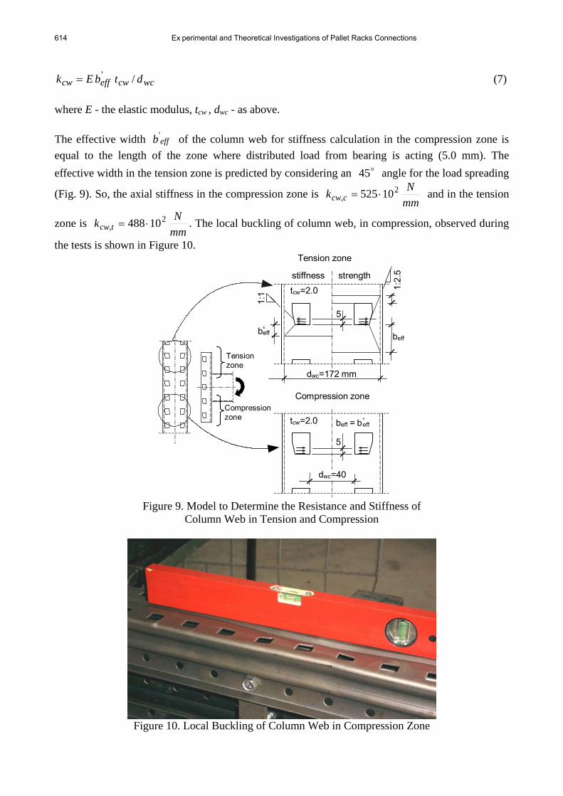
614 Ex perimental and Theoretical Investigations of Pallet Racks Connections
wccweffcw dtbEk /'= (7)
where E - the elastic modulus, tcw , dwc - as above. The effective width effb' of the column web for stiffness calculation in the compression zone is equal to the length of the zone where distributed load from bearing is acting (5.0 mm). The effective width in the tension zone is predicted by considering an o45 angle for the load spreading
(Fig. 9). So, the axial stiffness in the compression zone is mmNk ccw
2, 10525 ⋅= and in the tension
zone is mmNk tcw
2, 10488 ⋅= . The local buckling of column web, in compression, observed during
the tests is shown in Figure 10.
Compression zone
Tension zone
dwc=40
tcw=2.0
5
1:1
1:2.
5
beff beeffff ‘
dwc=172 mm
5
tcw=2.0
Tension zone
Compression zone
stiffness strength
beff = beff ‘
Figure 9. Model to Determine the Resistance and Stiffness of
Column Web in Tension and Compression
Figure 10. Local Buckling of Column Web in Compression Zone

Lucjan Ślęczka and Aleksander Kozłowski 615
3.1.4 Column web in shear Shear deformation of panel zone occurs only in case of external joints, when one-sided bending moment is acting from the beam. Shear force in panel zone is not uniformly distributed. Its values change in the levels of connector’s tabs (or levels of perforations in columns), see Figure 11. The highest value of shear force is reached at the center of the panel zone, while a small reductions occurs at its ends. For the sake of simplicity, it can be assumed that the shear force is uniformly distributed in the entire panel zone. Transformation parameter β accounting distribution of shear force at column length can in this case be calculated as (Faella et al. [18]):
c
p
hh
−= 1β (8)
where ph is the height of panel zone and ch is column height.
h1=19
h2=32
Tension zone
Compression zone
V
h p=2
00 m
m
V
V
hp hc
δ
Panel zone
Figure 11. Panel Zone in Shear
The resistance of panel zone in shear including the effect of the distribution of shear force is given by:
βscw
scwV
F ,, = (9)
where scwV , - resistance of column web in shear:
3,
,vccwy
scwAf
V = (10)
netvcA , is the shear area of column web, with accounting perforations of web. So the resistance of panel zone can be calculated as:
3,
, βvccwy
scwAf
F = (11)

616 Ex perimental and Theoretical Investigations of Pallet Racks Connections
The height of panel zone is equal to mmhp 200= , the column height in tested connections is
equal to mmhc 570= and 2, 106mmA netvc = , so 649.0=β and NF scw
3, 103,36 ⋅= .
The stiffness of panel zone is affected by the presence of perforations at regular intervals at column height. The axial stiffness of spring modeling behavior of this component has to be predicted from general rule, (Fig. 11):
δFk scw =, (12)
Deflection of panel zone under shear deformation δ can be predicted as the sum of deformation of areas with net shear area netvcA , and with gross shear area vcA :
vcnetvc AGhF
AGhF 2
,
1 ∑∑ +=δ (13)
where 1∑h and 2∑h are the total height of net shear area and gross shear area respectively. Taking into account that EG 38.0= and transformation parameter β accounting distribution of shear force at column length, equation (12) can be written as follow:
⎟⎟⎠
⎞⎜⎜⎝
⎛+
=∑∑
vcnetvc
scw
Ah
Ah
Ek2
,
1,
38.0
β
(14)
which gives value of axial stiffness mmNk scw /108,829 2, ⋅= .
Deformation of panel zone observed during the tests is shown in Figure 12.
Figure 12. Deformation of Panel Zone

Lucjan Ślęczka and Aleksander Kozłowski 617
3.1.5 Tabs in shear Another component affecting the rotational behaviour of the rack joint is the tab of the connector, subjected to bending and shear from local bearing stresses. To predict the resistance and stiffness of this component, the model of a cantilever beam subjected to a concentrated load can be used (Fig. 13). The distance between the load and fixed end of beam, measured by the developed length of tabs is equal mml 0,7= . The resistance of the tab stF , can be evaluated as shear resistance:
)3/( ,, couvst fAF = (15) where VA - effective shear area of tab; couf , - ultimate tensile stress of connector.
13
Area of bearing
Fl
ttab
Tension zone
Compr. zone
Figure 13. Tab in Shear and Bending
Because of the existence of undercuts in tabs, made during punching in time of production, effective thickness of tabs is equal mmt efftab 0,3, = , instead the nominal value mmt nomtab 0,4, = . The resistance is based on the ultimate tensile strength of the connector couf , rather than the yield
stress, so resistance of the component can be calculated as NF st3
, 101,9 ⋅= . The initial stiffness of this component stk , can be calculated using equation (2), where δ is the deflection of the beam (at the point where the concentrated load F is acting) from bending and shear:
FAG
lIE
l
V ⎟⎟⎠
⎞⎜⎜⎝
⎛+=
2.13
3δ (16)
Both moment of inertia I and shear area VA should be calculated taking into account the
effective thickness of the tabs. Using above equations, it can be predicted that mmNk st
2, 102714 ⋅= .
This component is active both in the tension and compression zones of the joint.

618 Ex perimental and Theoretical Investigations of Pallet Racks Connections
Deformations of tabs, due to shear and bending, observed during the tests are depicted in Figure 14.
Figure 14. Deformation of Tabs due to Shear and Bending
3.1.6 Connector in bending and shear Behaviour of the connector can be modelled taking into account a cantilevered part of the connector, protruding over the flange surface of the beam, as shown in Figure 15.
A A
A-A
δ
F
x
X
6 1337
70
4
Ext.
Int.
Figure 15. Connector in Bending and Shear

Lucjan Ślęczka and Aleksander Kozłowski 619
Resistance of the component can be found as plastic resistance of an element subjected to bending and shear:
NfAV coyVsco3
,, 102,193/ ⋅== (17)
mmNfWM coyplbco4
,, 1022,42 ⋅== . (18) where VA - effective shear area of connector; coyf , - yield stress of connector; plW - plastic section modulus of connector. The initial stiffness cok of this component is calculated as the ratio of the force to the deflection of the component under this force, equation (2). Because of the openings (slots) in connector, the deflection of the component was evaluated as for shear-wall structures containing openings under lateral loads according to (Benjamin [19]), including the effects of bending and shear. Every tested group of joints has different beam heights, so the initial stiffness of the component is different for each group. In every group, two values of initial stiffness have been calculated: for external slot (force is acting in tab more distant to the beam), and for internal slot (force is acting in tab closer to the beam). Predicted values of the initial stiffness for each group are listed below.
Group “B”: mmNk extco
2, 10540 ⋅= ,
mmNk tinco
2, 105664 ⋅= ;
Group “C”: mmNk extco
2, 10368 ⋅= ,
mmNk tinco
2, 102689 ⋅= ;
Group “E”: mmNk extco
2, 10662 ⋅= , ∞=tincok , .
For group “D” the values of initial stiffness of connector in bending and shear are the same as in group “B”, and for group “F” as in group “E”. This component is active both in the tension and compression zones of the joint. Observed deformations of connector during the test are shown in Figure 16.
Figure 16. Deformation of Connector Observed during the Tests

620 Ex perimental and Theoretical Investigations of Pallet Racks Connections
3.1.7 Connector web in tension (compression) Regarding the tension and compression zones of the connector web, the resistance cowF can be estimated according to (EN 1993-1-8 [14]) as:
coycoeffcow ftbF ,ω= (19) where ω - factor accounting for the interaction with shear; cot - thickness of the connector’s web,
cwyf , - yield stress of connector. The effective width of the connector web effb accounts for the spreading of the stresses transmitted by the beam flange (Figure 17). Assuming the tangent of the spreading angle 5.2:1 , effb =27 mm can be adopted and the resistance in compression and tension zones can be calculated as
NFF ccowtcow3
,, 104,37 ⋅== .
dwc=33
tco=4.0
b eff
33
Figure 17. Connector Web in Tension or in Compression
The axial stiffness of the connector web in tension and compression can be evaluated from the relationship:
wccoeffcow dtbEk /'= (20) Assuming an angle of o45 for the load spreading, the value of the initial stiffness
mmNkk ccowtcow
2,, 105760 ⋅== can be calculated.
3.1.8 Beam flange in tension (compression) The last component, beam flange in tension and compression, has to be considered only in the evaluation of the joint resistance. Its resistance can be computed as:
bfybfefftbfcbf ftbFF ,,, == (21)

Lucjan Ślęczka and Aleksander Kozłowski 621
where bft - thickness of the beam flange, bfyf , - yield stress of beam flange. The spreading of stresses to calculate the effective width of the beam effb is depicted in Figure 18. The value of
resistance in tension and compression zone can be predicted as NFF tbfcbf3
,, 109,29 ⋅== .
Weld toe
beff
Figure 18. Stress Distribution in the Beam Flange
3.2 Evaluation of the Rotational Stiffness The mechanical model adopted to predict the initial rotational stiffness is shown in Figure 19a. The springs representing the behaviour of the components are located at the level of the tabs of connector and at the level of beams flange. Only the lever arm of spring representing behaviour of panel zone is different. According to (EN 1993-1-8 [14]), it can conservatively be taken as the distance from centre of compression to a point midway between two rows of tabs in tension zone. In the calculation, it is also assumed that the contribution of the springs situated in the centre part of the joint is small and so their influence has been neglected.
a)
50
50
50
50
b)
c) d) e)
Sj,ini S1 S2
h b-t f
b
ht
hc h b-t f
b
kcw,tear
kcw,b
kcw,t
kcow,t
kcow,c
kco,ext
kco,int
kt,s
kcw,c
h b-t f
b
z p
kcw,s
50
50
50
50 z p
z p
S3
Figure 19. Mechanical Model and Procedure for Evaluating the Rotational Stiffness

622 Ex perimental and Theoretical Investigations of Pallet Racks Connections
The procedure to evaluate the rotational stiffness is depicted in Figures 19b - 19e. The first step is the computation of effective stiffness of each row (Fig. 19b), followed by the prediction of the equivalent overall stiffness in the compression and tension zones and of the lever arms (Fig. 19c). Third step is the change of two springs with axial stiffness into one spring with rotational stiffness (Fig. 19d); and finally the prediction of the initial stiffness of the whole model, (Fig. 19e). Adequate relationships to make conversion of mechanical model from Figure 19a to model depicted in Figure 19e can be found in mechanics handbooks or in (Faella et al. [18]). Presented model is general, spring representing panel behaviour is only active in external connections. In internal connections, panel zone is not affected by shear force and ∞=scwk , . The most influencing component on the rotational stiffness in tested connections is the column web in bearing. 3.3. Evaluation of the Flexural Resistance Behaviour of such joints can be considered in two stages: before direct contact of connector with column flange (elastic stage) and after this contact occurred (plastic stage). Mechanical model adopted to predict the elastic flexural resistance and lever arms for each group of components are presented in Figure 20a. Because the weakest component governs the resistance of each row, model depicted in Figure 20a can be easily simplified into model presented in Figure 20b.
50
50
50
50
a) b)
c)
h1
h2 hi
h b-t f
b
h b-t f
b
h b-t f
b
“1”
Mco,b ”3”
“2”
Fcw,tear
Fcw,b
Fcw,t
Fcw,c
Ft,s
Mco,b
Fcow,t
Fbf,c
Fcow,c
“1”
“2”
Mco,b
Fbf,t
z1
Z
Fcw,s
z p
50
50
50
50
z p
Fcw,s ”4”
Figure 20. Mechanical Models for the Elastic and Plastic Flexural Resistance Evaluation
The resistance of components marked “1” in Figure 20b is equal to NFF tearcw
3, 1036,6 ⋅==
when component is in tension (column web in tearing), or NFF bcw3
, 1007,8 ⋅== when component is in compression (column web in bearing). The resistance of components marked “2” (beam flange) is equal NFFF tbfcbf
3,, 109,29 ⋅=== and the resistance of the connector in

Lucjan Ślęczka and Aleksander Kozłowski 623
bending (modelled as rotational spring “3”) is equal to mmNM bco4
, 1022,42 ⋅= . The resistance of
column web in shear (“4”) is equal to NF scw3
, 103,36 ⋅= , but this component should be considered only in case of external connections. In internal connections, panel zone is not affected by shear force and ∞=scwF , . Model presented in Figure 20b represents only the initial behaviour of joint when the gap between the column flange and connector (Fig. 2) still exists. To describe ultimate behaviour of connection, it can be assumed that the rotation of the connector increases, the gap disappears and contact stresses start acting between column flange and connector directly, (Fig. 20c), what change the lever arm. Also, it is assumed that plastic distribution of internal forces can be obtained – the tests (Kozłowski and Ślęczka [13]) showed that all components have proper ductility. All forces acting in each row of components “1” in tension zone reach plastic capacity: minimum value between the resistance of their basic components -
NFF tearcw3
, 1036,6 ⋅== (column web in tearing). From condition of equilibrium, the reaction in compression zone Z is equal to the sum of forces in each tension rows. When the gap has disappeared, bearing stresses between connector and column are non-uniformly distributed. Because the flexural resistance of connector protruding over the flange surface of the beam cannot be exceeded, the centre of compression can be determined from equation:
ZM
z bco,1 = (22)
where Z = reaction force in compression zone, bcoM , = flexural resistance of connector and 1z = distance of centre of compression from bottom flange of beam, see Figure 20c. When the centre of compression is found, plastic flexural resistance can be predicted using equation:
bcoi
itearcwpl MhFM ,3
1, +∑=
= (23)
where ih = the distance of −i th component from the centre of compression, tearcwF , = minimum value of the resistance in each row (in this case column web in tearing) and bcoM , = flexural resistance of connector. In addition, the flexural resistance of upper part of connector should be checked. When the bending moment generated by two forces acting in upper rows is greater than the value of force acting in upper row, then the flexural resistance of connector bcoM , should be reduced to a value of tearcwF ,ψ in order to satisfy moment equilibrium. In case of external connections, plastic flexural resistance of connection could not be greater than the resistance of column web in shear: pscwpl zFM ,≤ . Figure 20c shows configurations of components only in internal connections. Component method shows that plastic flexural resistance of most joints (group “B”, “D”, “E” and “F”) is governed by the resistance of column web in tearing tearcwF , in tension zone and connector in bending and shear bcoM , in compression zone (Figure 21). Only in case of group “C”, the moment resistance is influenced by flexural resistance of connector bcoM , in tension zone, giving reduction of the force acting in the first row to tearcwF ,ψ (Figure 21).

624 Ex perimental and Theoretical Investigations of Pallet Racks Connections
Group “E” and “F”
70 12
0 170
120 65
22
Fcw,tear
Mco,b
60 100
110 16
0 75
22
Group “B” and “D”
Mco,b
Fcw,tear
80
150
100
60
25
85
Fcw,tear
ψ Fcw,tearGroup “C”
Mco,b
Plastic hinge
Figure 21. Plastic Resistance Model of Each Tested Joint Group 4. COMPARISON OF RESULTS Deformations of internal connectors observed during the tests are depicted in Figure 22 to compare with these from the proposed models, as shown in Figure 21. Collection of the resistances and stiffness of basic components, obtained using component method, is presented in Table 4. It can be seen that the weakest component in tension zone is column web in tearing, which the resistance is only NF tearcw
3, 1036,6 ⋅= . In compression zone, the weakest is
column web in bearing: NF bcw3
, 1007,8 ⋅= . The biggest influence on the joint global stiffness is the bearing of the tab to column web. These findings were confirmed during experimental tests and by the failure modes of joints, see Figures 6 and 8.
Figure 22. Typical Deformation of Internal Joints Observed in Each Joint Group

Lucjan Ślęczka and Aleksander Kozłowski 625
Table 4. Stiffness and Resistance of Analysed Joint Components
Component Axial stiffness ⎥⎦⎤
⎢⎣⎡mmN Resistance ][],[ NmmN
Column web in tearing 2, 105599 ⋅=tearcwk 3
, 1036,6 ⋅=tearcwF
Column web in bearing 2, 105,48 ⋅=bcwk 3
, 1007,8 ⋅=bcwF
Column web in tension 2, 10488 ⋅=tcwk 3
, 1025 ⋅=tcwF Column web in compression
2, 10525 ⋅=ccwk 3
, 102,42 ⋅=ccwF
Column web in shear 2, 108,829 ⋅=scwk 3
, 103,36 ⋅=scwF
Tabs in shear 2, 102714 ⋅=stk 3
, 101,9 ⋅=stF 2
, 10540 ⋅=extcok Group “B” and “D” 2
, 105664 ⋅=tincok 2
, 10368 ⋅=extcok Group “C” 2
, 102689 ⋅=tincok 2
, 10662 ⋅=extcok
Connector in
bending and shear
Group “E” and “F” ∞=tincok ,
3, 102,19 ⋅=scoV
4, 1022,42 ⋅=bcoM
Connector web in tension (compression)
2,, 105760 ⋅== ccowtcow kk 3
,, 104,37 ⋅== ccowtcow FF
Beam flange in tension (compression) -
3,, 109,29 ⋅== tbfcbf FF
Comparison of predicted by component method values of initial rotational stiffness with values from tests is shown in Table 5. Analytical values of plastic flexural resistance plM for all analysed groups and their comparison to values obtained during experimental tests are presented in Table 6.
Table 5. Prediction of the Initial Stiffness and Comparison with Experimental Data Test results
[kNm/rad] Component method
[kNm/rad]
Difference: (component-test)/test
[%] Group “B” Group “C” Group “D” Group “E” Group “F”
139,40 116,70 71,35
123,06 96,15
98,2 93,6 93,3
100,4 95,3
-29,6 -19,8 30,7
-18,4 -0,8

626 Ex perimental and Theoretical Investigations of Pallet Racks Connections
Table 6. Prediction of the Plastic Flexural Resistance and Comparison with Experimental Data Test results
[kNm] Component method
[kNm]
Difference: (component-test)/test
[%] Group “B” Group “C” Group “D” Group “E” Group “F”
3,19 2,36 3,10 3,20 3,37
2,95 2,49 2,95 3,13 3,13
-7,5 5,5
-4,8 -2,2 -7,1
Comparisons of predicted by means of the component method results with those obtained from tests shows the high level of accuracy, both for the stiffness and for the flexural resistance, in case of analysed joints. 5. CONCLUSIONS Behaviour of pallet rack joints is governed by a few components. Some of them are very similar to the components in structural connections of hot rolled I and H sections: column web in shear, column web in tension or in compression, beam flange in tension or in compression. Others are the result of using cold-formed perforated columns, special connectors and tabs in beam-column connection: tabs in shear, connector in bending and shear and column web in tearing. Analysis of behaviour of particular basic parts of the joints, like in component method, enable designers to understand joint performance and safety design. Next advantage of the component method is the possibility to predict mechanical characteristics of joints without expensive experimental work. Traditionally, the behaviour of such complex joints as steel pallet rack joints is predicted by testing. The component approach presented in the paper can be used as complementary method. Next important advantage of the component method is the possibility to provide clear and precise specification of the influence of each component on the resistance and stiffness of the joint. The weakest component can be easily identified and improved. It makes easier to conduct the optimisation of joints, especially in the systems, which are produced in long series, as steel storage pallet racks. Level of accuracy attained from component method shows the possibility of using this method in practical application.

Lucjan Ślęczka and Aleksander Kozłowski 627
REFERENCES [1] Abdel-Jaber, M., Beale, R.G., Godley, M.H.R, “Numerical Study on Semi-rigid Racking
Frames under Sway”, Computers and Structures, 2005, Vol. 83, pp. 2463–2475. [2] Beale, R.G., Godley, M.H.R., “Sway Analysis of Spliced Pallet Rack Structures”,
Computers and Structures, 2004, Vol. 82, pp. 2145–2156. [3] Bernuzzi, C., Castiglioni, C.A., “Experimental Analysis on the Cyclic Behaviour of
Beam-to-column Joints in Steel Storage Pallet Racks”, Thin-Walled Structures, 2001, Vol. 39, pp. 841–859.
[4] Freitas, A.M.S., Freitas, M.S.R., Souza, F.T., “Analysis of Steel Storage Rack Columns”, Journal of Constructional Steel Research, 2005, Vol. 61, No. 1135–1146.
[5] Godley, M.H.R., Beale, R.G., Feng, X., “Analysis and Design of Down-aisle Pallet Rack Structures”, Computers and Structures, 2000, Vol. 77, pp. 391-401.
[6] Peköz, T., Rao, K., “Design of Industrial Storage Racks”, Progress in Structural Engineering and Materials, 2001, Vol. 3, pp. 28-35.
[7] The, L.H., Hancock, G.J., Clarke, M.J., “Analysis and Design of Double-Sided High-Rise Steel Pallet Rack Frames”, Journal of Structural Engineering, July 1 2004, Vol. 130, No. 7, pp. 1011-1021.
[8] Baldassino, N., Zandonini, R., “Design by Testing of Steel Storage Pallet Racks”, Proceedings of the 3rd European Conference on Steel Structures, Coimbra, 2002, Vol. 1, pp. 689-698.
[9] Baldassino, N., Bernuzzi, C., “Analysis and Behaviour of Steel Storage Pallet Racks”, Thin-Walled Structures, 2000, Vol. 37, pp. 277–304.
[10] Markazi, F.D., Beale, R.G., Godley, M.H.R., “Experimental Analysis of Semi-Rigid Boltless Connectors”, Thin-Walled Structures, 1997, Vol. 28, No.1, pp. 57-87.
[11] Markazi, F.D., Beale, R.G., Godley, M.H.R., “Numerical Modelling of Semi-rigid Boltless Connectors”, Computers and Structures, 2001, Vol. 79, pp. 2391-2402.
[12] Institute of Logistics and Warehousing, “Safety of Storage Systems. Freestanding Racks. Basic requirements”, IL-B-001:1998 (in Polish).
[13] Kozłowski, A., Ślęczka, L., “Experimental Analysis of Beam-to-column Joints in Steel Storage Pallet Racks”, Proceedings of the 3rd European Conference on Steel Structures, Coimbra, 2002, Vol. II, pp. 897-906.
[14] EN 1993-1-8, Eurocode 3: Design of Steel Structures - Part 1.8: Design of Joints. CEN, Brussels, 2005.
[15] EN 1994-1-1. Eurocode 4: Design of Composite Steel and Concrete Structures. Part 1.1: General Rules and Rules for Buildings. CEN, Brussels, 2002.
[16] Fink, J., Rubin, D., Hollmann, K., “Anwendung des Innsbrucker Komponentenmodells bei der Optimierung eines modernen Deckenschaltischs“, Stahlbau 72, 2003, Heft 1.
[17] Chen, W.F., Newlin, D.E., “Column Web Strength of Beam-to-Column Connections”, Journal of the Structural Division, ASCE, 1973, Vol. 99, No. ST9.
[18] Faella, C., Piluso, V., Rizzano, G., “Structural Steel Semi rigid Connections, Theory, Design and Software”, CRC Press, 2000.
[19] Benjamin, J. R., “Statically Indeterminate Structures”, McGRAW-HILL, 1959.


![[Eng]Advanced Training Steel Connections 2008.0.1](https://img.pdfslide.us/doc/110x75/55cf9dca550346d033af34e4/engadvanced-training-steel-connections-200801.jpg)