Embed Size (px)
Citation preview
EUROPEAN ECONOMY
Economic Papers 471 | November 2012
Energy Inflation and House Price Corrections
Andreas Breitenfellner,Jesús CrespoCuaresma and Philipp Mayer
Economic and Financial Affairs
ISSN 1725-3187

Economic Papers are written by the Staff of the Directorate-General for Economic and Financial Affairs, or by experts working in association with them. The Papers are intended to increase awareness of the technical work being done by staff and to seek comments and suggestions for further analysis. The views expressed are the author’s alone and do not necessarily correspond to those of the European Commission. Comments and enquiries should be addressed to: European Commission Directorate-General for Economic and Financial Affairs Publications B-1049 Brussels Belgium E-mail: [email protected] This paper exists in English only and can be downloaded from the website ec.europa.eu/economy_finance/publications A great deal of additional information is available on the Internet. It can be accessed through the Europa server (ec.europa.eu) KC-AI-12-471-EN-N ISBN 978-92-79-22992-3 doi: 10.2765/27743 © European Union, 2012
European Commission
Directorate-General for Economic and Financial Affairs
Energy Inflation and House Price Corrections
By Andreas Breitenfellner 1, Jesús Crespo Cuaresma 2 and Philipp Mayer 3
EUROPEAN ECONOMY Economic Papers 471
1 European Commission, Brussels, Belgium (National Expert of Oesterreichische Nationalbank); Corresponding author ([email protected],eu).
2 Vienna University of Economics and Business, Vienna, Austria, Wittgenstein Centre for Demography and Global Human Capital, Vienna, Austria, International Institute for Applied Systems Analysis, Laxenburg, Austria, Austrian Institute of Economic Research, Vienna, Austria.
3 Erste Group, Vienna, Austria
Abstract We analyse empirically the role played by energy inflation as a determinant of downward corrections in
house prices. Using a dataset for 18 OECD economies spanning the last four decades, we identify periods of
downward house price adjustment and estimate conditional logit models to measure the effect of energy
inflation on the probability of these house price corrections after controlling for other relevant
macroeconomic variables. Our results give strong evidence that increases in energy price inflation raise the
probability of such corrective periods taking place. This phenomenon could be explained by various channels:
through the adverse effects of energy prices on economic activity and income reducing the demand for
housing; through the particular impact on construction and operation costs and their effects on the supply
and demand of housing; through the reaction of monetary policy on inflation withdrawing liquidity and
further reducing demand; through improving attractiveness of commodity versus housing investment on
asset markets; or through a lagging impact of common factors on both variables, such as economic growth.
Our results contribute to the understanding of the pass-through of oil price shocks to financial markets and
imply that energy price inflation should serve as an early warning indicator for the analysis of macro-
financial risks.
JEL classification: C33, G01, Q43, R21, R31
Keywords: Energy Prices, Housing Market, Financial Crisis, Conditional Logit Model
The authors thank Ismael A. Boudiaf for research assistance, as well as Christian Buelens, Björn Döring, Robert K. Kaufmann, Paul Kutos, Paul Pichler, Burkhard Raunig and Eric Ruscher for valuable suggestions. The views expressed in this paper are those of the authors and should not be attributed to the European Commission.
2
1. INTRODUCTION
Was it mere coincidence that the global financial crisis 2007-2009 occurred in proximity to
an oil shock? Between 2000 and mid-2008, the price of crude oil surged fivefold to an all-
time high of around USD 145 per barrel. Already one year before this peak the US subprime
mortgage crisis emerged, which led to the most severe financial crisis since the Great
Depression (Bernanke, 2010) and a truly global recession. Kaufmann et al. (2011) postulate a
direct role for energy prices in the 2008 financial crisis. Using cointegration methods, they
identify a significant long-run relationship between household expenditures on energy and
US mortgage delinquency rates. 1 Earlier research has already acknowledged that both
housing price corrections and energy price volatility are important determinants of recessions.
Leamer (2007) calculates that eight out of ten post-war recessions in the USA followed
shocks in the housing sector.2 According to Hamilton (2005), nine of these ten US recessions
were preceded by oil price shocks. With the recent Great Recession the relation to housing
price corrections gets augmented to 11 : 9 and to oil price shocks to 11 : 10 (Hamilton, 2010).
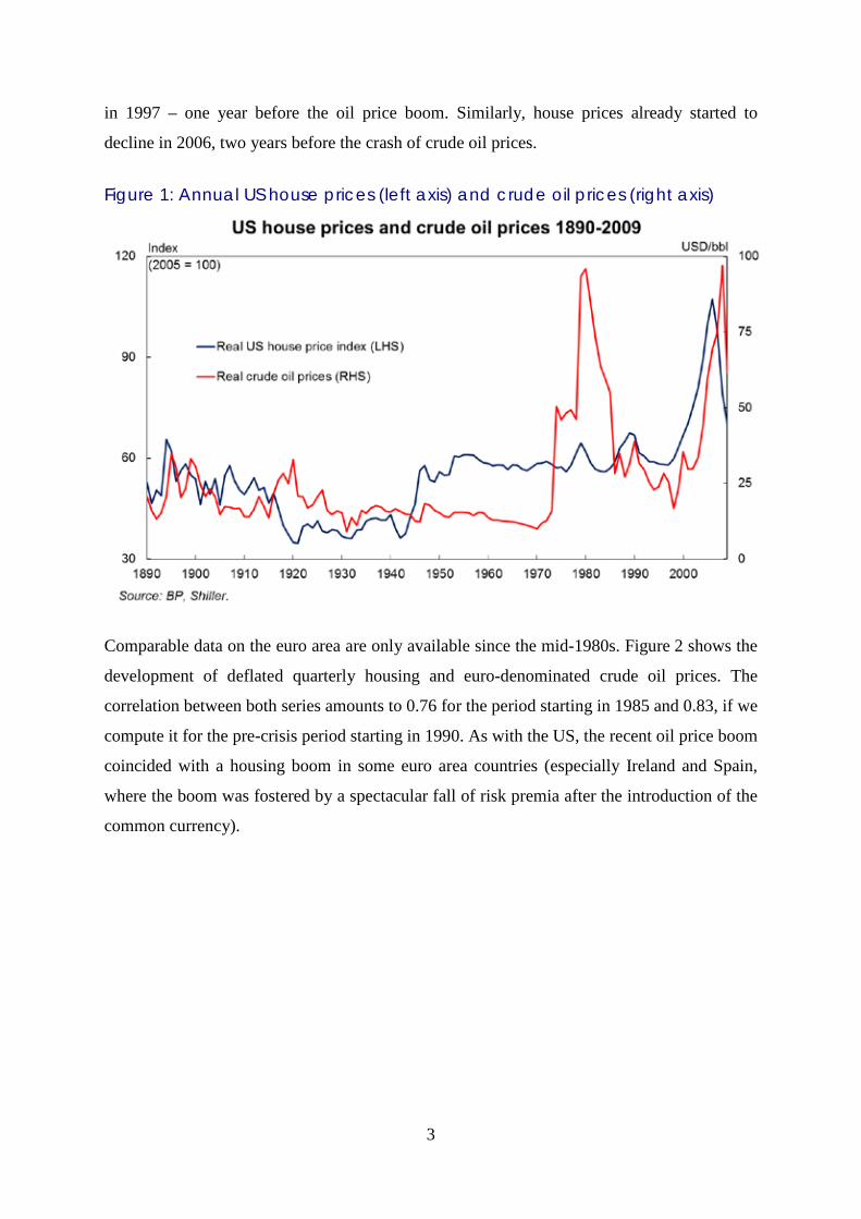
Inspection of historical data gives already a first illustration of the relationship between
energy and real estate markets. Figure 1 presents the annual development of real house and
crude oil prices in the US between 1890 and 2009. The correlation is not extraordinarily
strong over the whole period (0.52) but increases significantly during the last two decades. 3
The correlation between the post-1990 real oil price index and the real house price index in
the US is 0.72 and it increases to 0.93 between 2000 and 2006. Remarkable – from today's
perspective – are the modest drops of housing prices just in the initial phase of the two big oil
shocks of the past century (starting in 1972 and 1979) and after the first gulf war (1990/1). In
the period of oil price increases preceding the recent financial crisis, house prices accelerated
1 Campbell and Cocco (2011) show that adjustable-rate mortgages default tends to occur when inflation (which in the short-run is energy price driven) and nominal interest rates are high.
2 In its analysis of 19 advanced industrialized economies, IMF (2003) find that between 1970 and 2002 recessions tended to happen after an housing price bust, which all were followed by banking crisis.
3 The correlation of nominal house and crude oil prices is significantly higher (0.89). The use of real crude oil price data is convention in economic studies, although the typically high weight of energy prices in inflation would justify the use of nominal data.
3
in 1997 – one year before the oil price boom. Similarly, house prices already started to
decline in 2006, two years before the crash of crude oil prices.
Figure 1: Annual US house prices (left axis) and crude oil prices (right axis)
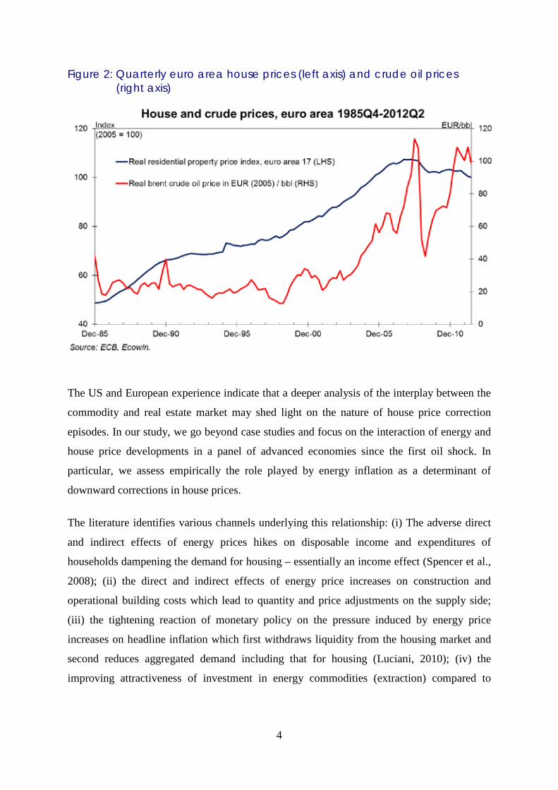
Comparable data on the euro area are only available since the mid-1980s. Figure 2 shows the
development of deflated quarterly housing and euro-denominated crude oil prices. The
correlation between both series amounts to 0.76 for the period starting in 1985 and 0.83, if we
compute it for the pre-crisis period starting in 1990. As with the US, the recent oil price boom
coincided with a housing boom in some euro area countries (especially Ireland and Spain,
where the boom was fostered by a spectacular fall of risk premia after the introduction of the
common currency).
4
Figure 2: Quarterly euro area house prices (left axis) and crude oil prices (right axis)
The US and European experience indicate that a deeper analysis of the interplay between the
commodity and real estate market may shed light on the nature of house price correction
episodes. In our study, we go beyond case studies and focus on the interaction of energy and
house price developments in a panel of advanced economies since the first oil shock. In
particular, we assess empirically the role played by energy inflation as a determinant of
downward corrections in house prices.
The literature identifies various channels underlying this relationship: (i) The adverse direct
and indirect effects of energy prices hikes on disposable income and expenditures of
households dampening the demand for housing – essentially an income effect (Spencer et al.,
2008); (ii) the direct and indirect effects of energy price increases on construction and
operational building costs which lead to quantity and price adjustments on the supply side;
(iii) the tightening reaction of monetary policy on the pressure induced by energy price
increases on headline inflation which first withdraws liquidity from the housing market and
second reduces aggregated demand including that for housing (Luciani, 2010); (iv) the
improving attractiveness of investment in energy commodities (extraction) compared to
5
housing on asset markets (Basu and Gavin, 2010); (v) the lagging impact of third common
factors on both variables, such as economic growth and monetary policy.
We use a panel of quarterly OECD data which spans over the period 1971-2008 for 18 OECD
member countries to test empirically whether changes in energy prices affect the probability
of house price adjustments. We control for a variety of relevant monetary, macroeconomic,
housing-market specific and demographic variables and account for misalignment of housing
prices from an estimated fundamental value. Our results confirm that changes in energy
inflation have a robust effect on house prices and in particular on the probability of
downward corrections. To our knowledge, this is the first study to assess this issue in a
rigorous econometric setting using longitudinal information from a broad group of
economies. Such an empirical strategy is particularly justified by the fact that house price
busts are often – but certainly not always – cross-border synchronized, presumably reflecting
synchronization of monetary policy, financial deregulation and business cycles (IMF, 2003).
In turn, energy price inflation is to a large extent determined by international oil price
developments, although rigidities in the pass-through of oil price shocks at the national level
may lead to sizeable differences in energy price dynamics across economies.
While the leading indicator quality of energy price inflation found in our study does not
exclude feedback effects in the opposite direction, the robustness and magnitude of the effect
of energy price inflation on house prices makes it relevant for policy considerations.
Assessing risks to price stability, energy prices are already well recognized as the most
important component of headline inflation volatility (ECB, 2010). Our findings imply that
monitoring of energy price developments should also be an important task for financial
market regulators and central banks in the framework of macro-financial risk assessment.4
The remainder of the paper is structured as follows: Section 2 discusses the relevant literature
and considers a few theoretical aspects. Section 3 tests our hypothesis empirically. Section 4
interprets the results and draws policy conclusions.
4 In early 2012, Eurostat, the statistical office of the European Union, started to publish a new house price index for its Macroeconomic Imbalance Procedure (MIP) Scoreboard. This set of indicators provides the basis for the economic reading of potential imbalances identified by the European Commission in its new annual Alert Mechanism Report. Apart from that Eurostat also runs pilot studies to capture price developments of owner-occupied housing (OOH), which is not included in the Harmonised Index of Consumer Prices (HICP).
6
2. OIL PRICES AND HOUSE PRICES: THEORETICAL LINKAGES
Several channels linking oil price developments and house prices have been identified in the
literature. In this section we summarize the existing theoretical frameworks related to such a
linkage. We build our survey about such mechanisms around the following channels: (i) an
income and demand channel, (ii) an energy related building cost channel, (iii) a monetary
policy channel, (iv) an asset price channel, and (v) via reversed causality or omitted factors.
2.1 INCOME AND DEMAND CHANNEL
Energy price inflation tends to reduce aggregate demand, and in particular housing demand.
This impact can be disentangled into a terms-of-trade effect, a demand-side and a supply-side
effect (ECB, 2010). First, the effect of oil price increases on terms of trade leads to a
reduction in purchasing power and wealth of households. Notwithstanding possible
adjustments of the saving rate, this would entail a reduction in consumption and (housing)
investment. Second, aggregated demand-side effects arise from inflation and its impact on
real income. Ideally, under perfect competition in labour and product markets, rising energy
prices would only lead to a relative price change, which could be compensated through
substitution for less energy-intensive demand. Rigidities, however, imply that energy prices
feed into headline inflation through first and second round effects. Third, supply-side effects
relate to the input costs of production. In the short-run, firms may react by either reducing
their profits or increase output prices, which in turn implies a reduction of consumption and
quantities produced. In the long-run, they would tend to substitute away from energy
intensive inputs.
Taken together, all these effects of oil price increases tend to depress income via decreased
purchasing power, profit squeeze and increasing unemployment. Hamilton (2009) as well as
Rubin and Buchanan (2008) explain the Great Recession as a result of oil price shocks, which
eventually contributed to bust the “house price bubble” 5 and triggered the financial crisis.6
5 The term “house price bubble” is widely accepted in the context of the most recent crisis (see e.g. Bernanke, 2010). Nevertheless, being aware of the general controversy over the term (Lind, 2009), we prefer to use the merely quantitative concept of “house price corrections”.
6 Explanations of recent global macroeconomic developments based on chronologies related to oil price changes are also put forward by Kilian (2009), Huntington (2005), Blanchard and Galí (2008) and Ramey and Vine (2010).
7
Due to the fact that the response of household spending not only reflects unanticipated
income changes but also a deterioration of consumer confidence leading to precautionary
savings (mainly at the cost of durables), the impact of an energy price shock on consumption
and housing investment is expected to be even higher than that on overall GDP (Edelstein
and Kilian 2009). Hamilton (2009) also argues that the recessionary effects of the oil shock
on income and unemployment depresses housing demand overproportionally. Such results
are in line with the high energy price elasticity estimates for residential investment
expenditures reported by Kilian (2008) that lead him to conclude that “energy price shocks
make themselves felt primarily through reduced demand for cars and new houses” (Kilian
2008, p. 889).
Microeconomic arguments which stress this connection have been put forward in the recent
literature. Relative to overall consumption, Cortright (2008) argues that fuel price increases
were at least partly responsible for the bursting of the recent US housing bubble and presents
evidence concerning the fact that house price declines were more severe in distant suburbs
that require lengthy commutes. The effect of gas prices on the demand for distant suburban
housing, reducing relative house prices in remote metropolitan areas, is thus put forward as a
mechanism linking oil price shocks to the end of the house price bubble.7
2.2 ENERGY RELATED BUILDING COST CHANNEL
Construction, maintenance and operation of buildings need energy. On the one hand, the
embodied energy is used for the extraction, processing and transport of building materials 8
as well as construction, maintenance and repair of the building. On the other hand, the
operational energy is used in providing the building services (heating, cooling, etc.) over its
lifetime9. This residential sector accounts for a quarter of overall energy consumption in
industrialized countries (Swan and Urgusal, 2009). Hence, the presumably negative effect of
7 Ramey and Vine (2010) summarize the adjustment behaviour of households in the US after permanent fuel price upsurges, first by reducing travel distances and in the longer run by revising their decision on where to live and work.
8 Time series of commodity prices (oil, metal, cement, etc.) generally tend to present a strong degree of co-movement.
9 The embodied energy accounts typically for between a sixth and a third of the total life-time energy consumption (Building Commission, 2006).
8
rising energy costs on housing demand and real estate prices can be sizable.10 Quigley (1984)
regards the production of housing service flows (i.e. the services households derive from the
dwellings they inhabit) and considers the demand for residential energy as a factor input.
Using production and demand functions for housing services, he estimates i.a. the elasticity
of substitution between operating inputs (largely energy) and real estate to be about 0.3.
According to those estimates, a doubling of energy prices is associated with an 11-15%
increase in the price of housing services, a decline of 7-10% in the demand for housing, and a
small increase in housing expenditures.
2.3 MONETARY POLICY CHANNEL
To the extent that energy price increases are passed through to medium-term headline or core
inflation, they may cause a restrictive monetary policy reaction. Higher interest rates have a
dampening effect on economic activity and household income, which tends to hit residential
investment over-proportionally (see the evidence in Edelstein and Kilian (2009)). Tight
monetary policy also reduces the inflow of liquidity to the housing sector just as low interest
rates tend to inflate house prices. Barsky and Kilian (2002) hold exogenous changes in
monetary policy chiefly responsible for historical stagflation episodes, which coincided with
the rise in oil prices. In addition, IMF (2008) suggests that house prices have become more
responsive to monetary policy innovations as a consequence of (flexible rate) mortgage
deregulation. With regard to residential investment, however, the impact of monetary policy
innovations has decreased since the mid-1980s, particularly in the US. Hence, more flexible
and developed housing finance appears to favour monetary policy transmission through
prices rather than investment in houses.
2.4 ASSET PRICE CHANNEL
Energy and housing-related securities compete for investment on asset markets. Increasing
energy prices attract investment to commodity producers that could otherwise flow into the
housing sector. Both asset markets serve as a hedge against inflation and safe haven when
inflation expectations are rising. Caballero et al. (2008) and El–Gamal and Jaffe (2010) 10 According to our back-of-the-envelope calculation (based on data from BP, US Census Bureau and Building Commission, 2006) total lifecycle energy costs of a typical one-family house in the US in relation to the respective total construction costs may have increased from below 6% of in 2004 to more than 9% in 2006 and around 15.5% in 2008.
9
provide a narrative of the evolution of the US house price boom as a consequence of
petrodollar recycling in the years before the subprime crisis.11 Rapid growth of emerging
economies and the associated rise in commodity prices induced capital flows from emerging
markets toward the US in search for (apparently) sound and liquid financial instruments (see
also Higgins et al., 2006). The exceptionally strong negative correlation between oil and
stock prices between July 2007 and June 2008 is put forward by Caballero et al. (2008) as
evidence for this interaction. After the burst of the housing bubble, the interaction between
housing, energy and financial markets continues to play an important role in explaining
current global developments. The crash exacerbated the scarcity of assets leading to a large
positive demand shock (which has sometimes been identified as a new bubble)12 in the oil
market, as well as markets for other commodities.
2.5 OMITTED FACTORS OR REVERSED CAUSALITY
Global liquidity, monetary policy, regulation and supervision of financial markets, as well as
overall cyclical dynamics may impact both energy and house prices, thus leading to joint
developments of these variables that may appear causal but are actually created by such a
third factor. Globally accommodative monetary conditions have been documented as a factor
driving commodity prices (Frankel, 2008) through a complex transmission mechanism. The
interest rate channel, on the one hand, affects commodity prices through its effect on
aggregate demand, inflation and incentives for producers to postpone extraction. The asset
market channel, on the other hand, changes incentives for financial market participants with
regard to risks or term structure, encouraging thus portfolio shifts or commodity carry trade
(G-20, 2011). 13 Monetary conditions, on the other hand, also impact real estate prices.
Utilizing structural VARs for several small open economies, Bjørnland and Jacobsen (2009)
present empirical evidence concerning the increasing role of house prices in the monetary
11 Looking at headline inflation in the US of the 1970s Piazzesi and Schneider (2012) show that the oil shock driven Great Inflation induced a portfolio shift by making housing more attractive than equity.
12 While there seems to be a consensus that the subprime crisis has been preceded by a housing bubble the notion of an "oil price bubble" has been much more disputed (Krugman, 2008) although some research would indeed suggest that oil price boom until 2008 went beyond fundamentals (Kaufmann, 2010).
13 Identifying these channels empirically and designating causalities is not trivial. Using a VAR model, Anzuini et al. (2010) present empirical evidence of a significant but weak relationship between an expansionary US monetary policy shocks and rising commodity prices. Erceg et al (2012), using their multi-country model SIGMA, show that "easy money in the dollar bloc" leads to a transitory run-up in oil prices.
10
transmission mechanism. Goodhart and Hoffman (2008) find evidence of a multidirectional
link between house prices, monetary variables and other macroeconomic variables. Such
results stand in contrast with those in Bernanke (2010), who finds that the direct linkages
between monetary policy and house price changes in the early part of the last decade were
weak.
Global demand certainly plays an important role for oil price developments (Hamilton 2009;
Kilian, 2009). This demand could originate from house price wealth effects – as expressed by
Leamer (2007), who states that "housing is the business cycle". The popular account of
financial crises by Reinhart and Reinhart (2010) also stresses the disastrous long-term impact
of real estate crashes on the economy. Spillovers from the housing sector to the rest of the
economy have widened through changes in housing finance systems in OECD economies
over the past two decades by supporting the use of housing as collateral (IMF, 2008).
3. EMPIRICAL ANALYSIS
In this section we assess empirically the role played by energy price inflation as a
determinant of house price corrections using a panel dataset spanning information for 18
OECD economies for the period 1971-2010 at a quarterly frequency. 14 Since our dependent
variable (the occurrence of a price reversal) is of a binary nature, we use conditional logit
specifications to model the process of house price reversals in our panel. The use of
conditional logit models allows for the inclusion of country-specific, time invariant factors
which control for fixed unobservable factors which may differ across economies. The logit
models used in the analysis are thus of the type
)+exp(+1)+exp(
=),|1=(ba
baa
iti
itiiitit x
xxyP , (1)
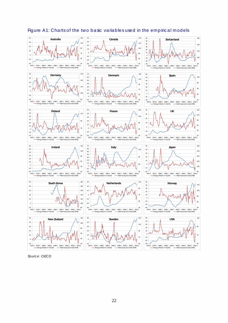
14 Energy inflation data (annual percentage change) is from the OECD Consumer Prices (MEI) dataset based on comparable national consumer price indices. The weight of energy is typically around a tenth in CPI baskets, roughly half of which is assigned to transportation fuels. The (not yet published) OECD cross-country dataset on house price indices is equally built on (mostly official) national sources with the intent of making them comparable. The countries in our sample are Australia, Canada, Denmark, Finland, France, Germany, Ireland, Italy, Japan, the Netherlands, New Zealand, Norway, Spain, South Korea, Sweden, Switzerland, US and UK. For closer data inspection see Figure A1 in the Appendix.
11
where yit takes value one if period t is a house price upward trend reversal period in country i
and zero otherwise and xit is a vector of determinants of house price reversals. Conditional
logit models of the type put forward in (1) can be estimated in a straightforward manner using
maximum likelihood methods (Chamberlain, 1980).
Answering our research question requires the identification of turning points in house price
data and the definition of periods corresponding to the price reversal. The recent empirical
literature on asset price bubbles (see Gerdesmeier et al., 2009, and Crespo Cuaresma, 2010)
follows variants of the approach proposed by Bry and Boschan (1971) in order to identify
peaks and troughs in house price data, which are used to date house price reversals. Starting
with the series of real house prices for a given country, pt, we define an observation as a
potential peak if it is a local maximum in a 6-quarter period (that is, pt-j< pt > pt+k for
j=1,…,3). Local minima are identified in a similar way and we impose a minimum length for
peak-to-trough/trough-to-peak phases of two quarters, as well as for full peak-to-peak and
trough-to-trough cycles of three years. Such a requirement ensures that our identified turning
points are not exclusively due to short-lived volatility in real estate prices. Following this
identification procedure, we define a house price reversal as the period corresponding to a
downward correction in house prices, as well as the previous and following quarter.15 The
dependent variable in our empirical model takes value one if the observation corresponds to a
correction period in the corresponding country, and zero otherwise. Table 1 presents the dates
corresponding to the identified house price turning points in the dataset. The procedure does
not detect any turning point in the house price series for Japan and the Netherlands, which are
therefore not included in the sample used to estimate the econometric models.
15 We define the correction period as in Crespo Cuaresma (2010), allowing thus for a certain degree of flexibility in identifying the actual starting point of the correction episode. In particular, the correction period is assumed to start one quarter before the peak (when the downward price pressures are supposed to be dominant), and last until the first quarter where such pressures are realized by the decrease in house prices.
12
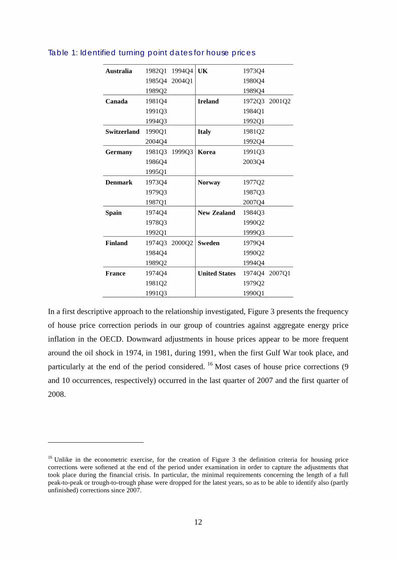
Table 1: Identified turning point dates for house prices
Australia 1982Q1 1994Q4 UK 1973Q4
1985Q4 2004Q1
1980Q4
1989Q2
1989Q4 Canada 1981Q4
Ireland 1972Q3 2001Q2
1991Q3
1984Q1
1994Q3
1992Q1 Switzerland 1990Q1
Italy 1981Q2
2004Q4
1992Q4 Germany 1981Q3 1999Q3 Korea 1991Q3
1986Q4
2003Q4
1995Q1 Denmark 1973Q4
Norway 1977Q2
1979Q3
1987Q3
1987Q1
2007Q4 Spain 1974Q4
New Zealand 1984Q3
1978Q3
1990Q2
1992Q1
1999Q3
Finland 1974Q3 2000Q2 Sweden 1979Q4
1984Q4
1990Q2
1989Q2
1994Q4 France 1974Q4
United States 1974Q4 2007Q1
1981Q2
1979Q2
1991Q3
1990Q1
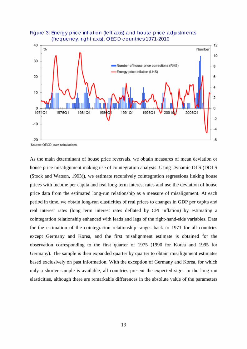
In a first descriptive approach to the relationship investigated, Figure 3 presents the frequency
of house price correction periods in our group of countries against aggregate energy price
inflation in the OECD. Downward adjustments in house prices appear to be more frequent
around the oil shock in 1974, in 1981, during 1991, when the first Gulf War took place, and
particularly at the end of the period considered. 16 Most cases of house price corrections (9
and 10 occurrences, respectively) occurred in the last quarter of 2007 and the first quarter of
2008.
16 Unlike in the econometric exercise, for the creation of Figure 3 the definition criteria for housing price corrections were softened at the end of the period under examination in order to capture the adjustments that took place during the financial crisis. In particular, the minimal requirements concerning the length of a full peak-to-peak or trough-to-trough phase were dropped for the latest years, so as to be able to identify also (partly unfinished) corrections since 2007.
13
Figure 3: Energy price inflation (left axis) and house price adjustments (frequency, right axis), OECD countries 1971-2010
As the main determinant of house price reversals, we obtain measures of mean deviation or
house price misalignment making use of cointegration analysis. Using Dynamic OLS (DOLS
(Stock and Watson, 1993)), we estimate recursively cointegration regressions linking house
prices with income per capita and real long-term interest rates and use the deviation of house
price data from the estimated long-run relationship as a measure of misalignment. At each
period in time, we obtain long-run elasticities of real prices to changes in GDP per capita and
real interest rates (long term interest rates deflated by CPI inflation) by estimating a
cointegration relationship enhanced with leads and lags of the right-hand-side variables. Data
for the estimation of the cointegration relationship ranges back to 1971 for all countries
except Germany and Korea, and the first misalignment estimate is obtained for the
observation corresponding to the first quarter of 1975 (1990 for Korea and 1995 for
Germany). The sample is then expanded quarter by quarter to obtain misalignment estimates
based exclusively on past information. With the exception of Germany and Korea, for which
only a shorter sample is available, all countries present the expected signs in the long-run
elasticities, although there are remarkable differences in the absolute value of the parameters
14
attached to the interest rate variable across countries. 17 The largest misalignments in the
sample are found for the UK and New Zealand in the period 2004-2007 (where prices are
estimated to deviate from the corresponding equilibrium by about 50%) and for Spain in the
eighties (with misalignments of around 45%).
In addition to energy price inflation, which is the central variable in our analysis, other
determinants of house price bubble bursts have been proposed in the literature and are added
to our set of covariates on the right hand side of (1). We choose variables which proxy
monetary policy and credit developments (credit growth, interest rate changes),
macroeconomic fundamentals (GDP per capita growth), housing market variables
(investment in housing, home ownership rates) and demographic dynamics (share of working
age population, population growth). Table 1 presents the estimation results of conditional
logit models of the form presented in (1) for different choices of control variables. All
specifications include decadal dummies and all explanatory variables are lagged one quarter
in order to ensure Granger-causal effects from the explanatory variables. The first column of
Table 2 presents the results from a bivariate model where the probability of house price
reversals is assumed to depend exclusively on energy price inflation. In this simple setting,
the results of the estimate indicate that increases in energy price inflation augment
significantly the probability of a price reversal. In this simple model the average marginal
effect of energy price inflation (evaluated assuming that the country fixed effect equals zero)
is 0.550, with a standard deviation of 0.0252. The effect of changes in energy price inflation
on the probability of house price adjustments is thus not only statistically significant, but also
sizable. Column 2 of Table 2 expands this simple specification by adding the house price
misalignment variable as a covariate in the model. As expected, the parameter associated to
this variable is estimated to be positive and highly significant, indicating that as house prices
increase above their equilibrium level the probability of a price reversal becomes higher. The
effect of energy price inflation remains positive and significant after controlling for the
misalignment level.
17 The estimated long-run elasticities which are used to obtain the measure of house price misalignments are presented in the Appendix, together with the source and descriptive statistics of all variables used in the econometric specifications.
15
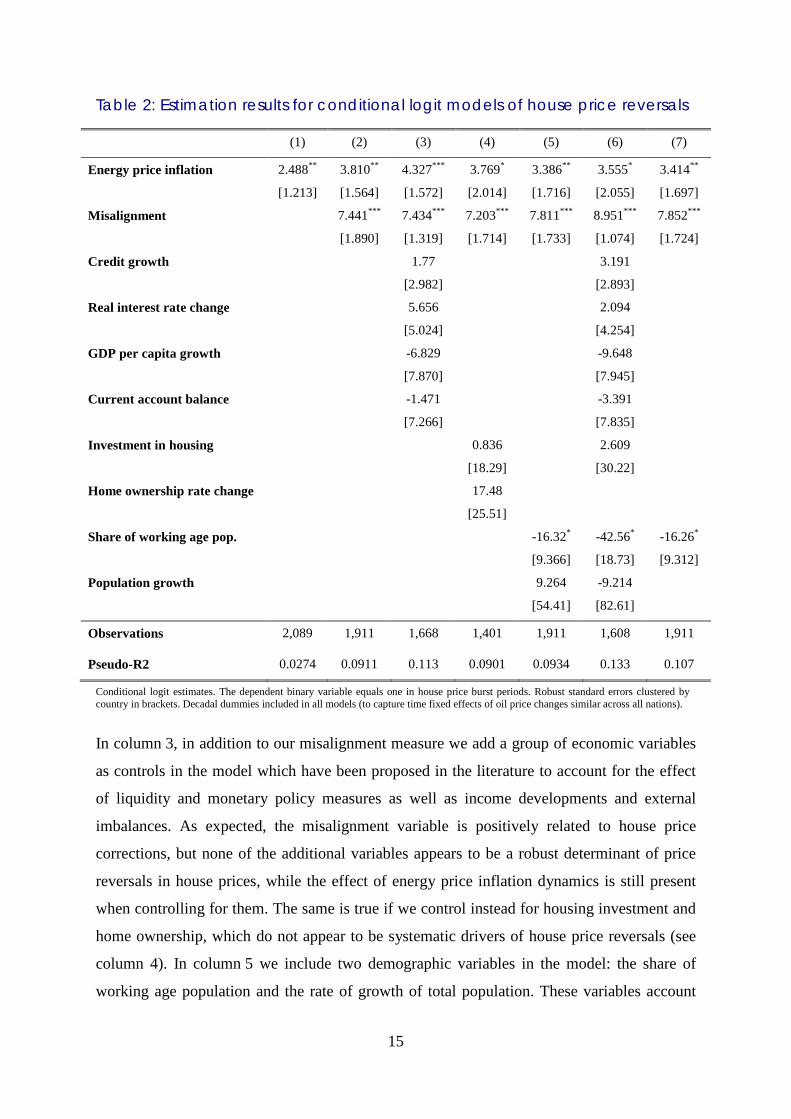
Table 2: Estimation results for conditional logit models of house price reversals
(1) (2) (3) (4) (5) (6) (7)
Energy price inflation 2.488** 3.810** 4.327*** 3.769* 3.386** 3.555* 3.414**
[1.213] [1.564] [1.572] [2.014] [1.716] [2.055] [1.697]
Misalignment 7.441*** 7.434*** 7.203*** 7.811*** 8.951*** 7.852***
[1.890] [1.319] [1.714] [1.733] [1.074] [1.724]
Credit growth 1.77 3.191
[2.982] [2.893]
Real interest rate change 5.656 2.094
[5.024] [4.254]
GDP per capita growth -6.829 -9.648
[7.870] [7.945]
Current account balance -1.471 -3.391
[7.266] [7.835]
Investment in housing 0.836 2.609
[18.29] [30.22]
Home ownership rate change 17.48
[25.51]
Share of working age pop. -16.32* -42.56* -16.26*
[9.366] [18.73] [9.312]
Population growth 9.264 -9.214
[54.41] [82.61]
Observations 2,089 1,911 1,668 1,401 1,911 1,608 1,911
Pseudo-R2 0.0274 0.0911 0.113 0.0901 0.0934 0.133 0.107
Conditional logit estimates. The dependent binary variable equals one in house price burst periods. Robust standard errors clustered by country in brackets. Decadal dummies included in all models (to capture time fixed effects of oil price changes similar across all nations).
In column 3, in addition to our misalignment measure we add a group of economic variables
as controls in the model which have been proposed in the literature to account for the effect
of liquidity and monetary policy measures as well as income developments and external
imbalances. As expected, the misalignment variable is positively related to house price
corrections, but none of the additional variables appears to be a robust determinant of price
reversals in house prices, while the effect of energy price inflation dynamics is still present
when controlling for them. The same is true if we control instead for housing investment and
home ownership, which do not appear to be systematic drivers of house price reversals (see
column 4). In column 5 we include two demographic variables in the model: the share of
working age population and the rate of growth of total population. These variables account
16
for potential effects of changes in the age structure of the population on the demand for
housing. Their inclusion does not affect the importance of energy prices and misalignments
as determinants of house price reversals. Furthermore, age structure dynamics as captured by
the share of working age population, potentially related to the probability of experiencing
turning points in house prices. Finally, the last column in Table 2 presents our preferred
model, where only significant variables from the specifications tried are considered. The
estimates of this model reaffirm the role of energy prices as an explanatory factor of house
price dynamics. The models estimated imply a marginal effect of energy price inflation on
the reversal probability between 0.5 and 0.6, depending on the specification used.
Several checks were carried out to ensure the robustness of our results. If contemporary
variables are considered instead of lagged covariates, the results presented in Table 2 are left
qualitatively unchanged, while the change in the real short term interest rate appears to be
significantly and positively related to turning point probabilities. The results for this variable,
which is meant to capture the role of monetary policy actions, indicate that monetary
tightening tends to be related to house price corrections, although establishing a causal
relationship between the two would require a more in-depth analysis that falls beyond the
scope of this study.
4. CONCLUDING REMARKS
This study empirically demonstrates a systematic relationship between energy and real estate
markets. The results of our analysis of 18 OECD countries over a period of 37 years confirm
the hypothesis that energy price inflation has significant leading indicator properties for
correction dynamics in house prices. Our estimated models imply that deviations from
fundamental-driven house prices play a significant role in such price corrections and thus
energy price inflation can be seen as playing a role in the bursting of house price bubbles.
Even without straightforward evidence of causality beyond the time lag structure used in the
specifications, we conclude from our results that energy price inflation can be considered an
important indicator not only for assessing challenges to price stability but also for financial
market stability.
Future research focused on the interactions of energy and real estate markets in a housing
boom phase appears important, as does a more systematic analysis of the reversed effect of
property price corrections on commodity price developments. Establishing an unequivocal
17
case for causality would probably require a thorough investigation of the channels sketched
in our study – a quite ambitious undertaking given the various cross-linkages involved.
Progress on this research agenda would provide inputs for the discussion on macro-financial
policies.
Various options are debated in order to minimize the probability or costs of excessive asset
price boom and bust cycles: (i) doing nothing and “cleaning up the mess” once the bubbles
burst; (ii) “leaning against the wind” via restrictive monetary policy; (iii) pursuing
contractionary fiscal policy and building up fiscal buffers; (iv) applying macro-prudential
measures to control household lending and improve bank resilience (Bernanke, 2010; Praet,
2010); (v) reforming regulation on the underlying real estate markets. 18 Our results suggest
that understanding the structure of energy markets might be particularly important for
monetary authorities as lower energy price volatility (G-20, 2011) and reduced energy
intensity (ECB, 2010) are important factors facilitating prudential macroeconomic policies.
18 Repealing mortgage deregulation and preferential (tax) treatment of homeownership could reduce house price volatility and hence the risks to macroeconomic stability (Andrews, et al., 2011). Chinese authorities, for instance, used farther-reaching regulatory measures to curb housing markets in recent years (Clemens et al., 2011). Furthermore, redirecting (zoning) policies towards “walkable cities” could also dampen the proliferation of car-dependent (and hence energy–intensive) suburban fringes (Leienberger, 2011).
18
REFERENCES
Andrews, D., A. Caldera Sánchez and Å. Johansson. 2011. Housing markets and structural policies in OECD countries. Economics Department Working Paper No. 836. Anzuini, A., M. J. Lombardi and P. Pagano. 2010. The impact of monetary policy shocks on commodity prices. ECB Working Paper 1232. Barsky, R. B. and L. Kilian. 2002. Do we really know that oil caused the great stagflation? A monetary alternative," in: NBER Macroeconomics Annual 2001/16: 137-198. Basu, P. and W. T. Gavin. 2010. What explains the growth in commodity derivatives? Review, Federal Reserve Bank of St Louis 93/1: 37-48.
Bernanke, B. S. 2010. Monetary policy and the housing bubble. Speech at the Annual Meeting of the American Economic Association, Atlanta, Georgia. January 3.
Bjørnland, H. C. and D. H. Jacobsen, 2009. The role of house prices in the monetary policy transmission mechanism in small open economies. Working Paper 2009/06, Norges Bank. Blanchard, O. and J. Galí. 2007. The macroeconomic effects of oil price shocks: Why are the 2000s so different from the 1970s? MIT Department of Economics Working Paper 0711.
Bry, G. and C. Boschan. 1971. Cyclical analysis of economic time series: Selected procedures and computer programs, NBER Technical Working Paper No. 20.
Building Commission. 2006. Energy impacts of different house types in Victoria. Melburne. www.buildingcommission.com.au. Campbell, J. Y. and J. F. Cocco. 2011. A model of mortgage default. NBER Working Paper 17516 .
Caballero R., E. Farhi and P. Gourinchas. 2008. Financial crash, commodity prices and global imbalances. NBER Working Paper 14521.
Clemens, U., S. Dyck and T. Just. 2011. China’s housing markets: Regulatory interventions mitigate risk of severe bust. Deutsche Bank Research, April.
Chamberlain, G. 1980. Analysis of covariance with qualitative data. Review of Economic Studies 47:225-238.
Cortright, J. 2008. Driven to the brink, how the gas price spike popped the housing bubble and devalued the suburbs, CEOs forCities. Mai.
Crespo Cuaresma, J. 2010, Can emerging asset price bubbles be detected? OECD Economics Department Working Papers 772.
ECB. 2010. Energy markets and the euro area macroeconomy. Occasional Paper Series 113, European Central Bank.
Edelstein, P. and L. Kilian. 2009. How sensitive are consumer expenditures to retail energy prices? Journal of Monetary Economics 56, 766–779.
El–Gamal, M.A. and Jaffe, A.M. 2010. Energy, financial contagion, and the dollar. Department of Economics, Rice University and James A. Baker III Institute for Public Policy. Working Paper.
Erceg, C., L. Guerrieri and S. B. Kamin. 2011. Did easy money in the dollar bloc fuel the oil price run-up? Working Paper. Federal Reserve Board.
19
Frankel, J. A. 2008. The effect of monetary policy on real commodity prices. In: Campbell, J. (Hg.). Asset Prices and Monetary Policy. NBER, University of Chicago Press.
G-20. 2011. Report of the G20 Study Group on Commodities, July.
Gerdesmeier, D., B. Roffia and H-E. Reimers. 2009. Asset price misalignments and the role of money and credit, ECB working paper 1068.
Goodhart, C. and B. Hofmann. 2008. House prices, money, credit and the macroeconomy. Oxford Review of Economic Policy 24: 180-205.
Hamilton, J. 2010. Nonlinearities and the macroeconomic effects of oil prices. Working Paper, Department of Economics, University of California, San Diego. Revised: June 14.
Hamilton, J. 2009. Causes and consequences of the oil shock of 2007-2008. Brooking Papers on Economic Activity.
Hamilton, J. 2005. Oil and the macroeconomy. Prepared for: Palgrave Dictionary of Economics.
Higgins, M., T. Klitgaard and R. Lerman. 2006. Recycling petrodollars. Current Issues in Economics and Finance 12/09. Federal Reserve Bank of New York.
Huntington, H. 2005. The economic consequences of higher crude oil prices. EMF Spezial Report 9. Stanford University.
IMF. 2008. The changing housing cycle and the implications for monetary policy. In: World Economic Outlook Washington, D.C, April: 103-132.
IMF. 2003. When bubbles burst. In: World Economic Outlook, Washington, D.C, April: 61-94.
Kaufmann, R. K. 2011. The role of market fundamentals and speculation in recent price changes for crude oil, Energy Policy 39/1: 105-115.
Kaufmann, R. K., N. Gonzalez, T. A. Nickerson and T. S. Nesbit. 2011. Do household energy expenditures affect mortgage delinquency rates? Energy Economics 33, 188–194.
Kilian, L. 2009. Not all oil price shocks are alike: Disentangling demand and supply shocks in the crude oil market. American Economic Review 99:3, 1053–1069.
Kilian, L. 2008. The economic effects of energy price shocks. Journal of Economic Literature, 46(4): 871–909.
Krugman, P. R. 2008. The oil nonbubble. New York Times. May 12. Leamer E. E. 2007. Housing is the business cycle. Proceedings, Federal Reserve Bank of Kansas City: 149-233.
Leinberger, C. 2011. The death of the fringe suburb. The New York Times, November 25.
Lind, H. 2009. Price bubbles in housing markets: Concept, theory and indicators. International Journal of Housing Markets and Analysis 2/1, 78 – 90.
Luciani, M. 2010. Monetary policy, the housing market and the 2008 recession: a structural factor analysis. Doctoral School of Economics, Sapienza University of Rome. Working Paper 7.
Quigley, J. M. 1984. The production of housing services and the derived demand for residential energy. Rand Journal of Economics. 15/4.
20
Piazzesi, M. and M. Schneider. 2012. Inflation and the Price of Real Assets. Working Paper, March 2012.
Praet, P. 2011. Housing cycles and financial stability – the role of the policymaker. Speech at the EMF Annual Conference, Brussels, 24 November. Ramey, V. and D. Vine. 2010. Oil, automobiles, and the US economy: How much have things really changed? NBER Working Paper No. 16067.
Reinhart, C. and V. Reinhart. 2010. After the fall. NBER Working Paper No. 16334.
Rubin, J. and P. Buchanan. 2008. What’s the real cause of the global recession? StrategEcon. CIBC World Markets Inc. 31. Oktober.
Spencer, T., L. Chancel and E. Guérin. 2012. Exiting the EU crises in the right direction: towards a sustainable economy for all. IDDRI Working Paper 09/ 12.
Stock J. and M. Watson, 1993. A simple estimator of cointegrating vectors in higher order cointegrated systems. Econometrica, 61, 783-820.
Swan, L. and V. I. Ugursal. 2009. Modeling of end-use energy consumption in the residential sector: A review of modeling techniques, Renewable and Sustainable Energy Reviews, 13/8: 1819-1835
21
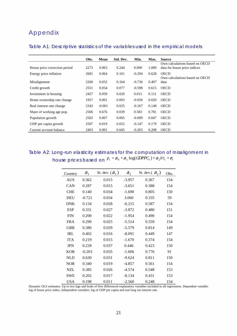
Appendix
Table A1: Descriptive statistics of the variables used in the empirical models
Obs. Mean Std. Dev. Min. Max. Source
House price correction period 2273 0.063 0.244 0.000 1.000 Own calculations based on OECD data for house price indices
Energy price inflation 2681 0.064 0.101 -0.294 0.628 OECD
Misalignment 2260 0.032 0.164 -0.736 0.497 Own calculations based on OECD data
Credit growth 2551 0.054 0.077 -0.598 0.615 OECD
Investment in housing 2457 0.059 0.020 0.015 0.151 OECD
Home ownership rate change 1957 0.001 0.003 -0.050 0.020 OECD
Real interest rate change 2343 -0.001 0.025 -0.167 0.148 OECD
Share of working age pop. 2506 0.676 0.039 0.583 0.781 OECD
Population growth 2502 0.007 0.005 -0.009 0.047 OECD
GDP per capita growth 2507 0.019 0.025 -0.147 0.179 OECD
Current account balance 2403 0.001 0.045 -0.203 0.208 OECD Table A2: Long-run elasticity estimates for the computation of misalignment in
house prices based on tttt lriGDPPCp eaaa ++)log(+= 210
Country 1a St. dev. ( 1a ) 2a St. dev.( 2a ) Obs. AUS 0.362 0.015 -3.957 0.367 154 CAN 0.287 0.015 -3.651 0.388 154 CHE 0.140 0.034 -1.690 0.805 150 DEU -0.721 0.034 3.060 0.335 59 DNK 0.134 0.028 -6.215 0.587 154 ESP 0.331 0.027 -3.872 0.480 151 FIN 0.200 0.022 -1.954 0.490 154 FRA 0.290 0.025 -5.514 0.559 154 GBR 0.380 0.029 -5.579 0.814 149 IRL 0.402 0.016 -8.091 0.449 147 ITA 0.219 0.015 -1.670 0.374 154 JPN 0.239 0.037 0.446 0.423 150 KOR -0.203 0.035 -1.606 0.776 91 NLD 0.630 0.031 -9.624 0.811 150 NOR 0.340 0.019 -4.857 0.561 154 NZL 0.385 0.026 -4.574 0.548 153 SWE 0.202 0.017 -8.134 0.431 153 USA 0.198 0.011 -2.560 0.248 154
Dynamic OLS estimates. Up to two lags and leads of first differenced explanatory variables included in all regressions. Dependent variable: log of house price index; independent variables: log of GDP per capita and real long run interest rate.
22
Figure A1: Charts of the two basic variables used in the empirical models
Source: OECD
30
50
70
90
110
130
-20
-10
0
10
20
30
40
1970:1 1975:1 1980:1 1985:1 1990:1 1995:1 2000:1 2005:1 2010:1
Australia
Energy inflation in % (LHS) Real house price index (RHS)
40
60
80
100
120
140
-30
-20
-10
0
10
20
30
40
1970:1 1975:1 1980:1 1985:1 1990:1 1995:1 2000:1 2005:1 2010:1
Canada
Energy inflation in % (LHS) Real house price index (RHS)
80
100
120
140
160
-30
-20
-10
0
10
20
30
40
50
60
1970:1 1975:1 1980:1 1985:1 1990:1 1995:1 2000:1 2005:1 2010:1
Switzerland
Energy inflation in % (LHS) Real house price index (RHS)
30
50
70
90
110
130
-10
0
10
20
30
40
50
60
70
1970:1 1975:1 1980:1 1985:1 1990:1 1995:1 2000:1 2005:1 2010:1
Denmark
Energy inflation in % (LHS) Real house price index (RHS)
20
40
60
80
100
-20
-10
0
10
20
30
40
50
60
1970:1 1975:1 1980:1 1985:1 1990:1 1995:1 2000:1 2005:1 2010:1
Spain
Energy inflation in % (LHS) Real house price index (RHS)
50
70
90
110
-20
-10
0
10
20
30
40
50
60
1970:1 1975:1 1980:1 1985:1 1990:1 1995:1 2000:1 2005:1 2010:1
Finland
Energy inflation in % (LHS) Real house price index (RHS)
40
60
80
100
120
-20
-10
0
10
20
30
40
50
1970:1 1975:1 1980:1 1985:1 1990:1 1995:1 2000:1 2005:1 2010:1
France
Energy inflation in % (LHS) Real house price index (RHS)
20
40
60
80
100
120
-20
-10
0
10
20
30
40
1970:1 1975:1 1980:1 1985:1 1990:1 1995:1 2000:1 2005:1 2010:1
UK
Energy inflation in % (LHS) Real house price index (RHS)
20
40
60
80
100
120
-20
-10
0
10
20
30
40
50
60
1970:1 1975:1 1980:1 1985:1 1990:1 1995:1 2000:1 2005:1 2010:1
Ireland
Energy inflation in % (LHS) Real house price index (RHS)
40
60
80
100
-20
-10
0
10
20
30
40
50
60
70
1970:1 1975:1 1980:1 1985:1 1990:1 1995:1 2000:1 2005:1 2010:1
Italy
Energy inflation in % (LHS) Real house price index (RHS)
80
100
120
140
160
180
-20
-10
0
10
20
30
40
50
1970:1 1975:1 1980:1 1985:1 1990:1 1995:1 2000:1 2005:1 2010:1
Japan
Energy inflation in % (LHS) Real house price index (RHS)
80
100
120
140
160
180
200
-10
0
10
20
30
40
50
1970:1 1975:1 1980:1 1985:1 1990:1 1995:1 2000:1 2005:1 2010:1
South Korea
Energy inflation in % (LHS) Real house price index (RHS)
30
50
70
90
110
-30
-20
-10
0
10
20
30
1970:1 1975:1 1980:1 1985:1 1990:1 1995:1 2000:1 2005:1 2010:1
Netherlands
Energy inflation in % (LHS) Real house price index (RHS)
40
60
80
100
120
-30
-20
-10
0
10
20
30
40
50
1970:1 1975:1 1980:1 1985:1 1990:1 1995:1 2000:1 2005:1 2010:1
Norway
Energy inflation in % (LHS) Real house price index (RHS)
50
70
90
110
-30
-20
-10
0
10
20
30
40
50
1970:1 1975:1 1980:1 1985:1 1990:1 1995:1 2000:1 2005:1 2010:1
USA
Energy inflation in % (LHS) Real house price index (RHS)
50
70
90
110
130
-10
0
10
20
30
40
50
1970:1 1975:1 1980:1 1985:1 1990:1 1995:1 2000:1 2005:1 2010:1
Sweden
Energy inflation in % (LHS) Real house price index (RHS)
20
40
60
80
100
120
-10
0
10
20
30
40
50
1970:1 1975:1 1980:1 1985:1 1990:1 1995:1 2000:1 2005:1 2010:1
New Zealand
Energy inflation in % (LHS) Real house price index (RHS)
90
100
110
120
130
-20
-10
0
10
20
30
40
1970:1 1975:1 1980:1 1985:1 1990:1 1995:1 2000:1 2005:1 2010:1
Germany
Energy inflation in % (LHS) Real house price index (RHS)

KC-AI-12-471-EN-N