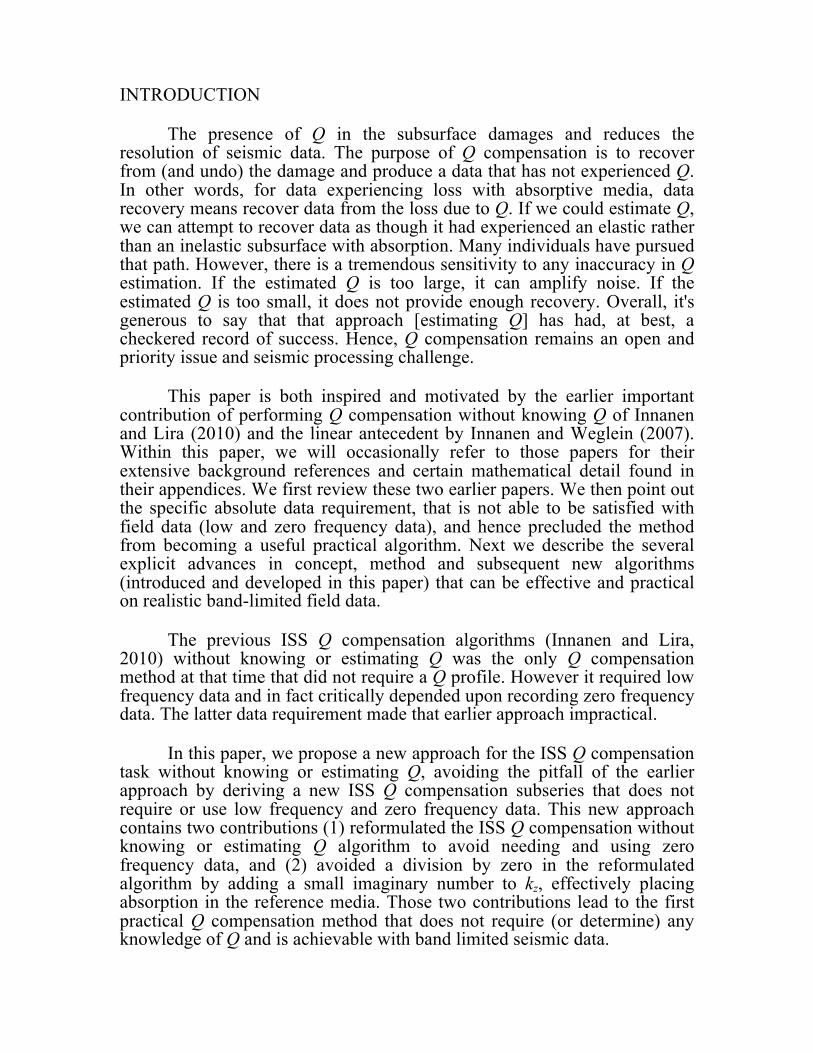
JOURNAL OF SEISMIC EXPLORATION 27, 593-608 (2018) 593

ISS Q COMPENSATION WITHOUT KNOWING, ESTIMATING OR DETERMINING Q AND WITHOUT USING OR NEEDING LOW AND ZERO FREQUENCY DATA YANGLEI ZOU and ARTHUR B. WEGLEIN M-OSRP, Physics Department, University of Houston, Houston, TX 77204, U.S.A. (Received June 2, 2018; revised version accepted October 12, 2018) ABSTRACT Zou, Y. and Weglein, A.B., 2018. ISS Q compensation without knowing, estimating or determining Q and without using or needing low and zero frequency data. Journal of Seismic Exploration, 27: 593-608. Developing new and more effective methods to achieve Q compensation is of priority in seismic processing and exploration. We propose a new approach for Q compensation as an isolated task subseries of the inverse scattering series (ISS). This inverse scattering subseries achieves Q compensation without needing to know, estimate or to determine Q. The method avoids the pitfall of an earlier ISS method by not needing or using low frequency data and in particular not needing zero frequency data. This paper provides two contributions (1) It develops a reformulated inverse scattering series (ISS) Q compensation method without knowing or estimating Q and (most importantly) without needing zero frequency data (2) It avoids a division by zero in the subsequent reformulated algorithm by adding a small imaginary term to kz (adding a small amount of friction in the reference medium). In this paper, we test the Q compensation algorithm in a two-reflector model and have obtained encouraging results. This advance in ISS Q compensation also has immediate significant and positive consequence for all amplitude analysis (that currently require low and zero frequency data) including ISS depth imaging, ISS direct parameter inversion, traditional iterative AVO and model matching FWI. In addition, the ISS Q compensation without knowing or estimating Q method can be transferred for electromagnetic applications where conductivity plays the role of Q, and a conductivity map can be output. Once the Q compensated data is available we could use that data together with the original data to estimate Q. Alternatively, the anelastic equation and data could input the original data and ISS inverted for elastic and Q parameters. KEY WORDS: Q compensation, inverse scattering Q compensation subseries, improved seismic resolution, direct inversion, target identification.

0963-0651/18/$5.00 © 2018 Geophysical Press Ltd.

INTRODUCTION The presence of Q in the subsurface damages and reduces the resolution of seismic data. The purpose of Q compensation is to recover from (and undo) the damage and produce a data that has not experienced Q. In other words, for data experiencing loss with absorptive media, data recovery means recover data from the loss due to Q. If we could estimate Q, we can attempt to recover data as though it had experienced an elastic rather than an inelastic subsurface with absorption. Many individuals have pursued that path. However, there is a tremendous sensitivity to any inaccuracy in Q estimation. If the estimated Q is too large, it can amplify noise. If the estimated Q is too small, it does not provide enough recovery. Overall, it's generous to say that that approach [estimating Q] has had, at best, a checkered record of success. Hence, Q compensation remains an open and priority issue and seismic processing challenge. This paper is both inspired and motivated by the earlier important contribution of performing Q compensation without knowing Q of Innanen and Lira (2010) and the linear antecedent by Innanen and Weglein (2007). Within this paper, we will occasionally refer to those papers for their extensive background references and certain mathematical detail found in their appendices. We first review these two earlier papers. We then point out the specific absolute data requirement, that is not able to be satisfied with field data (low and zero frequency data), and hence precluded the method from becoming a useful practical algorithm. Next we describe the several explicit advances in concept, method and subsequent new algorithms (introduced and developed in this paper) that can be effective and practical on realistic band-limited field data. The previous ISS Q compensation algorithms (Innanen and Lira, 2010) without knowing or estimating Q was the only Q compensation method at that time that did not require a Q profile. However it required low frequency data and in fact critically depended upon recording zero frequency data. The latter data requirement made that earlier approach impractical. In this paper, we propose a new approach for the ISS Q compensation task without knowing or estimating Q, avoiding the pitfall of the earlier approach by deriving a new ISS Q compensation subseries that does not require or use low frequency and zero frequency data. This new approach contains two contributions (1) reformulated the ISS Q compensation without knowing or estimating Q algorithm to avoid needing and using zero frequency data, and (2) avoided a division by zero in the reformulated algorithm by adding a small imaginary number to kz, effectively placing absorption in the reference media. Those two contributions lead to the first practical Q compensation method that does not require (or determine) any knowledge of Q and is achievable with band limited seismic data.

A REVIEW OF THE PREVIOUS ISS Q COMPENSATION WITHOUT KNOWING OR ESTIMATING Q ALGORITHM The Inverse-Scattering-Series (ISS) allows all seismic processing objectives, such as free-surface-multiple removal, internal-multiple removal, depth imaging, non-linear parameter estimation and Q compensation to be achieved directly in terms of data, and without any need to estimate or to determine subsurface properties. Weglein et al. (1997), Weglein et al. (2003) introduce the concept of isolated task subseries of the ISS to achieve those specific tasks. The recent ISS Q (compensation) without Q (estimation) algorithm (Innanen and Lira, 2010) provides a way to compensate Q in terms of only the data, without knowing, estimating or determining Q. This is a huge advantage especially for a complex subsurface where a Q profile is difficult or impossible to obtain. We will give a brief summary of their pioneering work. Starting from a non-absorptive wave equation for the reference medium ∇! + !!

!!!𝐺! 𝑥, 𝑥! ,𝜔 = 𝛿 𝑥 − 𝑥! , (1)

and a two-parameter (nearly constant Q) absorptive wave equation, where the physical properties only vary in depth, (Aki and Richards, 2002) ∇! + 𝑘! 𝐺! 𝑥, 𝑥! ,𝜔 = 𝛿 𝑥 − 𝑥! , (2) where, 𝑘 = !

! !1 + ! !

! ! and 𝐹 𝜔 = !

!− !

!𝑙𝑛 !

!! where 𝑐 𝑥 is a

spatially varying wave speed and 𝜔! is a chosen reference temporal frequency. Innanen and Lira (2010) treat the quantity in square brackets in equations 1 and 2 as the operators 𝐿! and 𝐿, respectively. By defining two perturbation quantities 𝛼 𝑥 = 1 − !!!

! ! ! and 𝛽 𝑥 = !!

, they arrive at a perturbation operator appropriate for this Q problem (for α <<1): 𝐿! − 𝐿 ≈

!!

!!!𝛼 𝑥 − 2𝐹 𝜔 𝛽 𝑥 = 𝑉 . (3)

Eqs. (1), (2) and (3) define the assumed physics model governing wave propagation in this paper. Following Weglein et al. (2003) we expand V as a series

𝑉 = 𝑉! + 𝑉! + 𝑉! +⋯ , (4) where Vn is the portion of V that is n-th order in the data. An inverse series for the perturbation V in terms of α and β is 𝛼 𝑧 − 2𝐹 𝜔 𝛽 𝑧 = 𝛼! 𝑧 − 2𝐹 𝜔 𝛽! 𝑧 + 𝛼! 𝑧 − 2𝐹 𝜔 𝛽! 𝑧 + ⋯ . (5) The inverse solution (e.g., Weglein et al., 2003) is generated by sequentially solving for V and summing contributions to the perturbation in orders of data, D (where D is the measured values of the scattered wavefield 𝐺 − 𝐺!). At first order, from 𝐺!𝑉!𝐺! = 𝐷 for 𝑉!we have 𝐷 𝑘! ,𝜃 = − !

!!"#! !𝑑𝑧!𝑒!!!!!! 𝛼! 𝑧! − 2𝐹 𝑘! ,𝜃 𝛽! 𝑧! , (6)

where the data D(xg,t), for one shot record, is first Fourier transformed over 𝑥! and 𝑡 to find 𝐷 𝑘! ,𝜔 [𝑥!is the receiver coordinate and 𝑡 is time]. Then changing variables and defining 𝑘! ≡ 2𝑞! = 2 𝑘! − 𝑘!! with k = ω/c0 and 𝑞! = 𝜔/𝑐 𝑐𝑜𝑠 𝜃 . With the assumption that the data contains only primaries, Innanen and Lira (2010) found a closed-form for a selected set of (partial) contributions to 𝑉 = !!

!!![𝛼 𝑥 − 2𝐹 𝜔 𝛽 𝑥 ] benefiting from an analogous

ISS depth imaging subseries of Shaw and Weglein (2003) and Shaw (2005)

𝛼! 𝑘! − 2𝐹 𝑘! ,𝜃 𝛽! 𝑘!

= 𝑑𝑧!𝑒!!!![!!!

!!!"#!(!) !!!! !! !!! !!! ! !! !!!

!!! ]

𝛼! 𝑧!

− 2𝐹 𝜔 𝛽! 𝑧! (7) where 𝛼! 𝑧 = 𝛼!!! 𝑧!

!!! and 𝛽! 𝑧 = 𝛽!!! 𝑧!!!! . The quantities

αn and βn are the contributions to α and β, that are nth order in the data D. F has been written as a function of the reference plane-wave variables θ and kz rather than ω (Please see Innanen and Lira, 2010 Appendix B for a detailed derivation). The goal of Innanen and Lira (2010) is to carry out a single isolated task, that of compensation for Q, and to ultimately output data that would not have experienced Q. The principle role of α1 in the argument of the exponential is to nonlinearly accomplish aspects of the inversion associated with wave speed deviations between the reference and actual media. Those tasks include internal multiple removal and depth imaging and amplitude analysis.

The role of β in the forward series is responsible for all the Q effects on the data. Thus in the inverse series, the 𝛽! is responsible for Q compensation, or data recovery. More precisely, the role of 𝛽! in the inverse series is to accomplish aspects of the inversion associated with deviations between reference (𝑄 = ∞) and actual Q values. Following this observation, Innanen and Lira (2010) proposed an approximate form of Q compensation algorithm by isolating terms in the inverse series that related to 𝛽! (which is responsible for Q compensation) and avoiding 𝛼! only and 𝛼! and 𝛽! coupled terms, output (a leading order capture of isolated 𝛽! inverse series) 𝛼! 𝑘! − 2𝐹 𝑘! ,𝜃 𝛽! 𝑘!

= 𝑑𝑧!𝑒!!!![!!!

! !!,!!"#!(!) !!!! !! !!!

!!! ]

𝛼! 𝑧! − 2𝐹 𝜔 𝛽! 𝑧!

(8)

and the Q compensated data or recovered data is

𝐷!"#$ 𝑘! ,𝜃 = − !!!"#! !

𝛼! 𝑘! − 2𝐹 𝑘! ,𝜃 𝛽! 𝑘! , (9)

where the original input data is

𝐷 𝑘! ,𝜃 = − !!!"#! !

𝛼! 𝑘! − 2𝐹 𝑘! ,𝜃 𝛽! 𝑘! . (10)

More terms related to Q compensation could be isolated and more accurate algorithms could be proposed in the future analogous to higher order ISS imaging subseries HOIS (Liu et al., 2004, 2005b; Liu, 2006; Wang et al., 2010a,b; Wang and Weglein, 2011; Wang, 2012), that can accommodate larger 1/Q values and larger regions where 𝑄 ≠ ∞. Another advantage of this algorithm is that it is formulated and operates in the data domain instead of the model domain [similar to the ISS free-surface multiple elimination algorithm (Carvalho, 1992; Weglein et al., 1997) and the ISS internal multiple attenuation algorithm (Araújo et al., 1994; Weglein et al., 1997, 2003)] making the algorithm more robust to noise and bandwidth issues. However, similar to the ISS depth imaging subseries (Shaw, 2005; Weglein et al., 2003; Liu et al., 2004, 2005a) the previous ISS Q compensation without knowing or estimating Q algorithm (Innanen and Weglein, 2007; Innanen and Lira, 2010) has a practical issue and shortcoming in that it requires low and zero frequency data which is not achievable with field data. In this paper a new starting point, and concomitant algorithm, specifically designed to avoid the need for that unachievable low and zero

frequency data, is developed providing a new and practical ISS Q compensation algorithm, without knowing or estimating Q, while avoiding the pitfall of the earlier approach for ISS Q compensation. The new algorithm provided in the next section of this paper does not require or use low frequency data and has absolutely no interest in or need for zero frequency data. This new approach contains two contributions (1) reformulated the ISS Q compensation without knowing or estimating Q algorithm to avoid using zero frequency data, and (2) avoided division by zero in the reformulated algorithm by adding a small imaginary number to kz. In the next section, we will discuss the two contributions and advances in this paper, in detail.

REFORMULATING 1D PRESTACK ISS Q COMPENSATION WITHOUT KNOWING OR ESTIMATING Q AND WITHOUT USING OR NEEDING LOW/ZERO FREQUENCY DATA As we discussed in the last section, Innanen and Lira (2010) provides an ISS Q compensation without knowing or estimating Q algorithm for a 1D subsurface, with offset data, and Innanen and Weglein (2007) provided the linear relationship and starting point. The Q compensated data (𝐷!"#$) which is the data without suffering Q, can be obtained by compensating the data experiencing Q as following, 𝐷!"#$ 𝑘! ,𝜃 =

− !!!"#! !

𝑑𝑧!𝑒!!!![!!!! !!,!

!"#!(!) !!!! !! !!!!!! ] 𝛼! 𝑧! − 2𝐹 𝑘! ,𝜃 𝛽! 𝑧!

(11)

and the original data (D) experiencing Q is related to 𝛼! and 𝛽! by the following equation, 𝐷 𝑘! ,𝜃 = − !

!!"#! !𝑑𝑧!𝑒!!!!!! 𝛼! 𝑧! − 2𝐹 𝑘! ,𝜃 𝛽! 𝑧! , (12)

where 𝛼! and 𝛽!are linear approximations of (i.e. the portion that is linear in data) 𝛼 = 1 − !!!

! ! ! and 𝛽 𝑥 = !!

respectively. 𝐹 𝑘! ,𝜃 = !!− !

!𝑙𝑛 ! !!,!

!!

where 𝜔 𝑘! ,𝜃 = − !!!!!!"#$

and the reference frequency 𝜔! is a component of the A-D model, which in our numerical studies we choose to be the highest

frequency in a given experiment, D is the reflection data we obtained from a subsurface with absorption, and the 𝐷!"#$ is the data after Q compensation. To calculate 𝐷!"#$, we need 𝛽! 𝑧 . Innanen and Weglein (2007) proposed and described in detail how to estimate β1 as a function of pseudodepth z. Eq. (10) can be rewritten as follows, 𝛼! 𝑘! − 2𝐹 𝑘! ,𝜃 𝛽! 𝑘! = −4𝑐𝑜𝑠! 𝜃 𝐷 𝑘! ,𝜃 . (13) To solve for 𝛽!, Innanen and Weglein (2007) use the data at two incidence angles, 𝐷 𝑘! ,𝜃! and 𝐷 𝑘! ,𝜃! , where 𝜃 = 𝑐𝑜𝑠!! 𝑘!𝑐!/2𝜔 , as follows 𝛼! 𝑘! − 2𝐹 𝑘! ,𝜃! 𝛽! 𝑘! = −4𝑐𝑜𝑠! 𝜃! 𝐷 𝑘! ,𝜃! , (14) and 𝛼! 𝑘! − 2𝐹 𝑘! ,𝜃! 𝛽! 𝑘! = −4𝑐𝑜𝑠! 𝜃! 𝐷 𝑘! ,𝜃! , (15) and then solve for 𝛽!. This results in 𝛽! 𝑘! = 2 ! !!,!! !"#! !! !! !!,!! !"#! !!

! !!,!! !! !!,!! . (16)

Similarly, we can solve eqs. (14) and (15) for α1. Then 𝛼!and 𝛽! can be used in eq. (9) for Q compensation. This is the previous ISS Q compensation without knowing or estimating Q algorithm. However, as we mentioned, there is an issue in this earlier approach. In eqs. (14) and (15) the solutions for 𝛼! 𝑘! and 𝛽! 𝑘! require knowledge of data 𝐷 𝑘! ,𝜃 at 𝑘! = 0, which corresponds (for any fixed 𝜃) to 𝜔 = 0. Furthermore in eq. (8), the integral of the 𝛽! 𝑧!! (in the e exponential 𝑑𝑧!!!!

! 𝛽! 𝑧!! ) is very sensitive to low and zero frequency in the data. Therefore, the zero 𝑘! value of 𝛽! depends on the 𝜔 = 0 component of the data (𝐷 𝑘! ,𝜃! and 𝐷 𝑘! ,𝜃! ). The requirement of low and zero frequency data made those earlier approaches impractical. For prestack data, and an assumed one dimensional subsurface, β1 will be a one dimensional function of kz and the data is a two dimensional function of (kz,θ). Thus there is one free parameter in the data. Any choice of the free parameter will give a different β1, as it should, and a different ISS Q compensation subseries will be responsible for Q compensation. We

reformulated the equations for calculating β1 from the kz, θ domain to the kz, kx domain. Two kx values will solve for α1 and β1 and for each two specific values will have a different solution for α1 and β1 and a distinct ISS Q compensation subseries. When kx is relatively small, the reformulated equations will provide a similar α1 or β1 looking result as we can obtain in the kz, θ domain. However, this reformulation will avoid the requirement of zero frequency data in the previous algorithm for α1 or β1 and the subsequent Q compensation subseries. If the selected kx values are not small the α1 and β1 will not provide a similar appearing result as we obtain in the kz, θ domain (more detailed discussion in Appendix B), a different subseries that is responsible for Q compensation (or ISS imaging for α1) needs to be identified and isolated, which will be pursued and progressed in future work. Thus in order to estimate β1, we reformulated eqs. (14) and (15),

𝛼!(𝑘!) − 2𝐹(𝑘! , 𝑘!!)𝛽!(𝑘!) = −4 !!!

!!!!!!!! 𝐷(𝑘! , 𝑘!!) , (17)

and

𝛼! 𝑘! − 2𝐹 𝑘! , 𝑘!! 𝛽! 𝑘! = −4 !!!

!!!!!!!! 𝐷 𝑘! , 𝑘!! . (18)

Eq. (16) becomes

𝛽! 𝑘! = 2! !!,!!!

!!!

!!!!!!!! !! !!,!!!

!!!

!!!!!!!!

! !!,!!! !! !!,!!! . (19)

Eq. (19) uses data at two different 𝑘! values instead of data at two

different angles. Since 𝜔/𝑐! = 𝑘!!! + 𝑞!! for 𝐷(𝑘! , 𝑘!!) and 𝜔/𝑐! =

𝑘!!! + 𝑞!! for 𝐷(𝑘! , 𝑘!!), the 𝑘! = 0 component of 𝛽! is no longer related

to ω = 0 component of the data, thus avoiding the pitfall of requiring zero frequency data (now the 𝑘! = 0 in 𝛽! is related to 𝜔/𝑐! = 𝑘! in the data). That is, 𝐷(𝑘! ,𝜔) with 𝑘! = 𝜔/𝑐! will provide the 𝑘! = 0 in β1(kz).

The Q compensation formula [eq. (9)] becomes, 𝐷!"#$ 𝑘! , 𝑘! =

− !!∫ 𝑑𝑧! !!

!!!!!

!!!𝑒!!!! !!!

!!!!!!! ! !!,!!!!!

!!!!! !!!!! 𝛼! 𝑧! – 2𝐹 𝑘! , 𝑘! 𝛽! 𝑧! .

(20)

In eqs. (17) and(18), the required data at 𝑘! = 0 is no longer related to requiring data at ω = 0. However, in the new reformulated ISS Q compensation algorithm [eq. (20)] 𝑘! appears in the denominator and division by 𝑘! = 0 is not defined. To avoid division by zero, we add a small imaginary number (adding a small amount of friction in the reference) to 𝑘! so that the denominator will not be zero. This is the second contribution in this work. Eqs. (17)-(20) provide the new and practical ISS Q compensation algorithm that inputs data, 𝐷(𝑥! , 𝑡), one shot record [for a 1D subsurface], a data that has suffered damage due to absorption, and outputs a data 𝐷!"#$(𝑥! , 𝑡) with the damage due to Q removed. This algorithm is a first order inverse scattering subseries with higher order subseries required for: (1) larger values of 1/Q and (2) cases where the region that the data experiences Q is larger. Extensions for a multidimensional 2D and 3D acoustic subseries are clear (and will be necessary) and further developments and contributions for an anelastic multidimensional subsurface are planned.

There are positive benefits from the approach and contribution in this paper for all seismic processing methods that currently require low and zero frequency data. Among the latter methods are AVO, and non-linear iterative AVO, FWI and ISS direct depth imaging without a velocity model. In particular the approach in this paper could be used in the ISS imaging sub-series to avoid the need for zero frequency data. A discussion can be found in Appendix A.

There are two ways that the method described in this paper could be

used to estimate Q: (1) the relationship between Dcomp and D could be used to determine Q, and (2) a parameter estimation series for 𝛽!, 𝛽!, 𝛽!,… could be computed to determine 𝛽(𝑟) = ∑𝛽!(𝑟) and Q. Neither of these Q determination methods would require low or zero frequency data.

This new Q compensation method assumes that the input data consists

of primaries, and hence that the reference wave, all ghosts, and all multiples have been removed from the recorded data. These event removal steps are essential prerequisites for this methodology. In addition, the data used in this Q compensation algorithm, 𝐷(𝑘! ,𝜔), where for a fixed 𝑘! we use the data such that 𝜔 ≥ 𝑘! to avoid evanescent waves. Evanescent waves are not needed in this algorithm.

This advance in ISS Q compensation also has immediate positive and

consequential implication and application to electromagnetic (EM) probes, where EM target identification interests and activities would welcome determining a conductivity map. A conductivity map can be used to separate brine water from hydrocarbons.

For example, the wave equation for the electric field in a conducting

material is

𝛻!𝐸 − 𝜇𝜎𝐸 − 𝜇𝜖𝐸 = 0 . (21) A plane wave solution to the wave equation is

𝐸(𝑟, 𝑡) = 𝐸!𝑒!(!"!!⋅!)𝑒!!⋅! , (22)

where |𝛼| = 𝜔 𝜇𝜖[!!+ !

!1 + !!

!!!!]! !, 𝛽 = !"#

!!, σ is the conductivity of

the material, µ is the permeability and ε is the permittivity.

There is a similarity between the EM waves propagating in a conducting medium and the seismic waves in an absorptive medium. The

second exponential factor, 𝑒!!⋅! , gives an exponential decay in the amplitude of the wave. Therefore, the current Q compensation method provided in this paper could also be used for EM waves in a conducting medium.

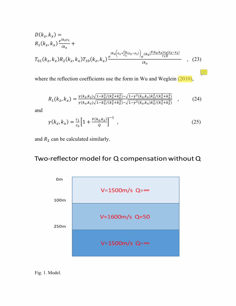
The ability to remove the effects of absorption will enhance the high frequency components of the data. The recently developed first migration method that is equally effective at all frequencies at the target [Weglein et al. (2016) and Weglein (2018)] will enhance the low frequency contributions for specular and non-specular target resolution and identification. Taken together they will improve both the low and high end frequency components of a target image and the resolving power of a probing wavefield and, e.g., they have the potential to advance medical imaging and to aid early cancer detection. We plan to pursue the latter broad band target resolution enhancement for medical imaging. A 1D PRESTACK NUMERICAL TEST FOR ISS Q COMPENSATION WITHOUT KNOWING OR ESTIMATING Q AND WITHOUT USING OR NEEDING LOW/ZERO FREQUENCY DATA In this section, we test the new algorithm for a 1D prestack two reflector model as shown in Fig. 1. The data is generated analytically (only primaries) in the 𝑘!,𝑘! domain using the following analytic form,

𝐷 𝑘! , 𝑘! =𝑅! 𝑘! , 𝑘!

!!!!!!

!!!+

𝑇!" 𝑘! , 𝑘! 𝑅! 𝑘! , 𝑘! 𝑇!" 𝑘! , 𝑘!!!!! !!!

!!!!

!!!!!!! !!

! !!,!! !! !!!!!!!!

!!! , (23)

where the reflection coefficients use the form in Wu and Weglein (2010),

𝑅!(𝑘! , 𝑘!) =!(!!,!!) !!!!!/(!!!!!!!)! !!!!(!!,!!)!!!/(!!!!!!!)!(!!,!!) !!!!!/(!!!!!!!)! !!!!(!!,!!)!!!/(!!!!!!!)

, (24)

and

𝛾 𝑘! , 𝑘! = !!!!1 + ! !!,!!

!

!! , (25)

and 𝑅! can be calculated similarly.

Fig. 1. Model.

Fig. 2 (left) shows the data from the model with Q, (middle) shows that data after being processed by the new ISS Q without Q subseries, and (right) shows data from the model that has no Q.

Fig. 2. Left: Data generated by the model with Q. Middle: The data (with Q) after ISS Q compensation without knowing or estimating Q Right: Data generated by the same model but without Q.

The single trace comparison of this new algorithm show an effective Q compensation without knowing or needing Q and without low frequency data. Of course these results can be used to estimate Q (which can have its own value) once you know how data with Q would look without Q.

Fig. 3. One trace comparison. Red line: Data with Q. Green line: Data with Q after Q compensation. Blue line: Data without Q.

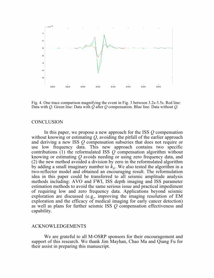
Fig. 4. One trace comparison magnifying the event in Fig. 3 between 3.2s-3.5s. Red line: Data with Q. Green line: Data with Q after Q compensation. Blue line: Data without Q. CONCLUSION In this paper, we propose a new approach for the ISS Q compensation without knowing or estimating Q, avoiding the pitfall of the earlier approach and deriving a new ISS Q compensation subseries that does not require or use low frequency data. This new approach contains two specific contributions (1) the reformulated ISS Q compensation algorithm without knowing or estimating Q avoids needing or using zero frequency data, and (2) the new method avoided a division by zero in the reformulated algorithm by adding a small imaginary number to 𝑘!. We also tested the algorithm in a two-reflector model and obtained an encouraging result. The reformulation idea in this paper could be transferred to all seismic amplitude analysis methods including: AVO and FWI, ISS depth imaging and ISS parameter estimation methods to avoid the same serious issue and practical impediment of requiring low and zero frequency data. Applications beyond seismic exploration are discussed (e.g., improving the imaging resolution of EM exploration and the efficacy of medical imaging for early cancer detection) as well as plans for further seismic ISS Q compensation effectiveness and capability. ACKNOWLEDGEMENTS We are grateful to all M-OSRP sponsors for their encouragement and support of this research. We thank Jim Mayhan, Chao Ma and Qiang Fu for their assist in preparing this manuscript.

REFERENCES Aki, K. and Richards, P.G., 2002. Quantitative Seismology. 2nd ed. University Science Books, Sausalito. Araújo, F.V., Weglein, A.B., Carvalho, P.M. and Stolt, R.H., 1994. Inverse scattering series for multiple attenuation: An example with surface and internal multiples. Expanded Abstr., 64th Ann. Internat. SEG Mtg., Los Angeles: 1039–1041. Carvalho, P.M., 1992. Free-surface Multiple Reflection Elimination Method Based on Nonlinear Inversion of Seismic Data. Ph.D. thesis, Universidade Federal da Bahia, Salvador. Innanen, K.A. and Lira, J.E., 2010. Direct nonlinear Q-compensation of seismic primaries reflecting from a stratified, two-parameter absorptive medium. Geophysics, 75: V13-V23. Innanen, K.A. and Weglein, A.B., 2007. On the construction of an absorptive-dispersive medium model via direct linear inversion of reflected seismic primaries. Inverse Probl., 23: 2289-2310. Liu, F., Nita, B.G., Weglein, A.B. and Innanen K.A., 2004. Inverse Scattering Series in the Presence of Lateral Variations. M-OSRP Ann. Report 3. Liu, F., Weglein, A.B, Innanen, K.A. and Nita, B.G., 2005. Extension of the non-linear depth imaging capability of the inverse scattering series to multidimensional media: strategies and numerical results. Abstr., 9th Internat. Congr. Braz. Geophys. Soc.: 2257-2261. Liu, F., 2006. Multi-dimensional depth imaging without an adequate velocity model. Ph.D. thesis, University of Houston. Liu, F., Weglein, A.B., Innanen, K.A. and Nita. B.G., 2005. Inverse scattering series for vertically and laterally varying media: application to velocity independent depth imaging. M-OSRP 2004-2005 Ann. Report: 176–263. Shaw, S.A., 2005. An inverse scattering series algorithm for depth imaging of reflection data from a layered acoustic medium with an unknown velocity model. Ph.D. thesis, University of Houston. Shaw, S.A. and Weglein, A.B., 2003. Imaging seismic reflection data at the correct depth without specifying an accurate velocity model: Initial examples of an inverse scattering subseries. In: Chen, C.H. (Ed.), Frontiers of Remote Sensing Information Processing. World Scientific Publishing Company: 469-484. Wang, Z. and Weglein, A.B., 2011. An investigation of ISS imaging algorithms beyond HOIS, to begin to address exclusively laterally varying imaging challenges. M-OSRP 2010-2011 Ann. Report: 105- 114. Wang, Z., Weglein, A.B. and Liu. F., 2010. Note: A derivation of the HOIS closed form. M-OSRP 2009- 2010 Ann. Report.: 118-125. Wang, Z., Weglein, A.B. and Liu, F., 2010. Note: Evaluations of the HOIS closed form and its two variations. M-OSRP 2009-2010 Ann. Report.: 126-136. Wang, Z., 2012. Progressing Inverse Scattering Series Depth Imaging Without the Velocity Model for Larger Contrast and Laterally Variable Media. Ph.D. thesis, University of Houston. Weglein, A.B., Gasparotto, F.A., Carvalho, P.M. and Stolt. R.H., 1997. An inverse-scattering series method for attenuating multiples in seismic reflection data. Geophysics, 62: 1975-1989. Weglein, A.B., Araújo, F.V., Carvalho, P.M., Stolt, R.H., Matson, K.H., Coates, R.T., Corrigan, D., Foster, D.J., Shaw, S.A. and Zhang, H., 2003. Inverse scattering series and seismic exploration. Inverse Probl., 19: R27-R83. Weglein, A.B., Mayhan, J., Zou, Y., Fu, Q., Liu, F., Wu, J., Ma, C., Lin, X. and Stolt, R.H., 2016. The first migration method that is equally effective for all acquired frequencies for imaging and inverting at the target and reservoir. Expanded Abstr., 86th Ann. Internat. SEG Mtg., Dallas: 4266-4272. Weglein, A.B., 2018. Direct and indirect inversion and a new and comprehensive perspective on the role of primaries and multiples in seismic data processing for structure determination and amplitude analysis, CT&F - Ciencia de Tecnologia y Futuro. In press. Wu, J. and Weglein, A.B., 2014. The first test and evaluation of the inverse scattering series internal multiple attenuation algorithm for an attenuating medium. Expanded Abstr., 84th Ann. Internat. SEG Mtg., Denver: 4130-4134.

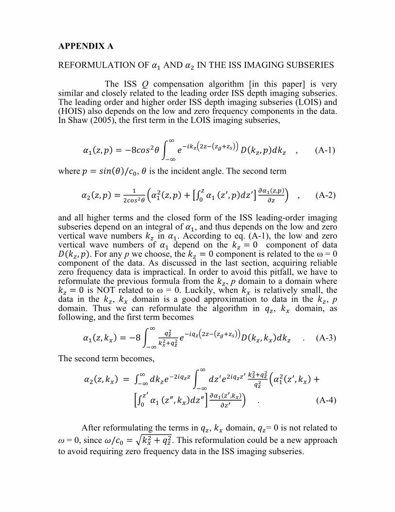
APPENDIX A REFORMULATION OF 𝛼! AND 𝛼! IN THE ISS IMAGING SUBSERIES

The ISS Q compensation algorithm [in this paper] is very similar and closely related to the leading order ISS depth imaging subseries. The leading order and higher order ISS depth imaging subseries (LOIS) and (HOIS) also depends on the low and zero frequency components in the data. In Shaw (2005), the first term in the LOIS imaging subseries,

𝛼! 𝑧, 𝑝 = −8𝑐𝑜𝑠!𝜃 𝑒!!!! !!! !!!!!!

!!𝐷 𝑘! , 𝑝 𝑑𝑘! , (A-1)

where 𝑝 = 𝑠𝑖𝑛 𝜃 /𝑐!, 𝜃 is the incident angle. The second term 𝛼! 𝑧, 𝑝 = !

!!"!!!𝛼!! 𝑧, 𝑝 + 𝛼!

!! 𝑧!, 𝑝 𝑑𝑧! !!! !,!

!" , (A-2)

and all higher terms and the closed form of the ISS leading-order imaging subseries depend on an integral of 𝛼!, and thus depends on the low and zero vertical wave numbers 𝑘! in 𝛼!. According to eq. (A-1), the low and zero vertical wave numbers of 𝛼! depend on the 𝑘! = 0 component of data 𝐷(𝑘! , 𝑝). For any p we choose, the 𝑘! = 0 component is related to the ω = 0 component of the data. As discussed in the last section, acquiring reliable zero frequency data is impractical. In order to avoid this pitfall, we have to reformulate the previous formula from the 𝑘!, p domain to a domain where 𝑘! = 0 is NOT related to ω = 0. Luckily, when 𝑘! is relatively small, the data in the 𝑘!, 𝑘! domain is a good approximation to data in the 𝑘!, p domain. Thus we can reformulate the algorithm in 𝑞!, 𝑘! domain, as following, and the first term becomes

𝛼! 𝑧, 𝑘! = −8 !!!

!!!!!!!

!

!!𝑒!!!! !!! !!!!! 𝐷 𝑘! , 𝑘! 𝑑𝑘! . (A-3)

The second term becomes,

𝛼! 𝑧, 𝑘! = 𝑑𝑘!𝑒!!!!!!!!! 𝑑𝑧!𝑒!!!!!! !!

!!!!!

!!!𝛼!! 𝑧!, 𝑘! +

!

!!

𝛼!!!

! 𝑧!, 𝑘! 𝑑𝑧!!!! !!,!!

!!! . (A-4)

After reformulating the terms in 𝑞!, 𝑘! domain, 𝑞!= 0 is not related to ω = 0, since 𝜔/𝑐! = 𝑘!! + 𝑞!!. This reformulation could be a new approach to avoid requiring zero frequency data in the ISS imaging subseries.

APPENDIX B

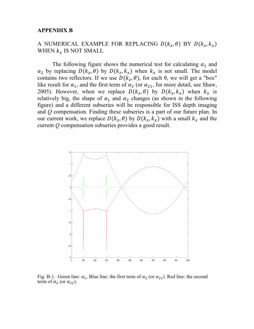
A NUMERICAL EXAMPLE FOR REPLACING 𝐷(𝑘! ,𝜃) BY 𝐷(𝑘! , 𝑘!) WHEN 𝑘! IS NOT SMALL

The following figure shows the numerical test for calculating 𝛼! and 𝛼! by replacing 𝐷(𝑘! ,𝜃) by 𝐷(𝑘! , 𝑘!) when 𝑘! is not small. The model contains two reflectors. If we use 𝐷(𝑘! ,𝜃), for each θ, we will get a "box" like result for 𝛼!, and the first term of 𝛼! (or 𝛼!", for more detail, see Shaw, 2005). However, when we replace 𝐷(𝑘! ,𝜃) by 𝐷(𝑘! , 𝑘!) when 𝑘! is relatively big, the shape of 𝛼! and 𝛼! changes (as shown in the following figure) and a different subseries will be responsible for ISS depth imaging and Q compensation. Finding these subseries is a part of our future plan. In our current work, we replace 𝐷(𝑘! ,𝜃) by 𝐷(𝑘! , 𝑘!) with a small 𝑘! and the current Q compensation subseries provides a good result.

Fig. B-1. Green line: 𝛼!, Blue line: the first term of 𝛼! (or 𝛼!"). Red line: the second term of 𝛼! (or 𝛼!!).