Ispd-2007

Repeater Insertion for Repeater Insertion for Concurrent Setup and Hold Time Violations Concurrent Setup and Hold Time Violations

with Power-Delay Trade-Offwith Power-Delay Trade-Off

Salim Chowdhury John LillisSalim Chowdhury John Lillis Sun Microsystems University of Illinois at ChicagoSun Microsystems University of Illinois at Chicago

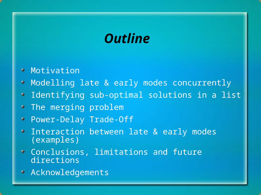
Outline

Motivation

Modelling late & early modes concurrently

Identifying sub-optimal solutions in a list

The merging problem

Power-Delay Trade-Off

Interaction between late & early modes (examples)

Conclusions, limitations, and future directions

Acknowledgements

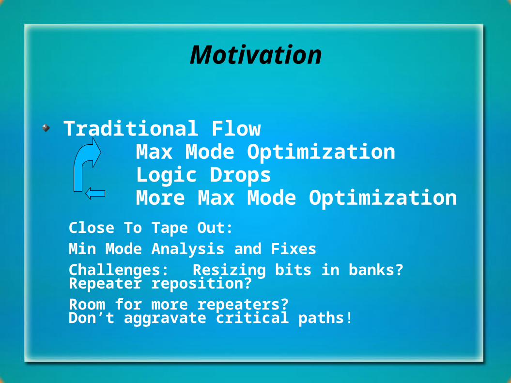
Motivation

Traditional FlowMax Mode OptimizationLogic DropsMore Max Mode Optimization

Close To Tape Out:Min Mode Analysis and FixesChallenges: Resizing bits in banks?

Repeater reposition?Room for more repeaters?Don’t aggravate critical paths!

Outline

Motivation

Modelling late & early modes concurrently

Identifying sub-optimal solutions in a list

The merging problem

Power-Delay Trade-Off

Interaction between late & early modes (examples)

Conclusions, limitations, and future directions

Acknowledgements

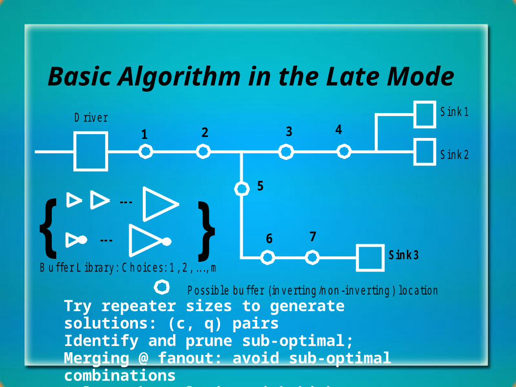
Basic Algorithm in the Late Mode

Try repeater sizes to generate solutions: (c, q) pairsIdentify and prune sub-optimal; Merging @ fanout: avoid sub-optimal combinationsSelect the solution with highest q @ driver

D ri v e r

P o s s i b l e b u f fe r ( in v e r t i n g /n o n - i n v e r ti n g ) l o c a ti o n

S i n k 1

S i n k 2

Sink3

-- -

-- -{ }B u ffe r L i b ra r y : C h o i c e s : 1 , 2 , . . . , m

1 2 3 4

5

6 7

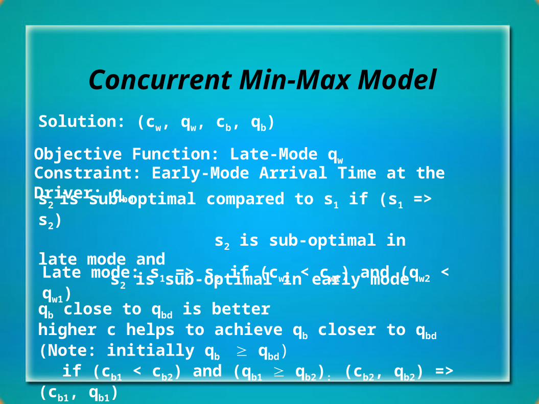
Concurrent Min-Max Model

qb close to qbd is betterhigher c helps to achieve qb closer to qbd (Note: initially qb qbd)

if (cb1 < cb2) and (qb1 qb2): (cb2, qb2) => (cb1, qb1)

Objective Function: Late-Mode qw

Constraint: Early-Mode Arrival Time at the Driver: qbd

s2 is sub-optimal compared to s1 if (s1 => s2) s2 is sub-optimal in late mode and

s2 is sub-optimal in early mode

Solution: (cw, qw, cb, qb)

Late mode: s1 => s2 if (cw2 < cw1) and (qw2 < qw1)

Outline

Motivation

Modelling late & early modes concurrently

Identifying sub-optimal solutions in a list

The merging problem

Power-Delay Trade-Off

Interaction between late & early modes (examples)

Conclusions, limitations and future directions

Acknowledgements

Pruning a List of SolutionsFour rules: cw2 cw1 in all cases:Case I: qb1 > qbd and qb2 qbd:

Case II: qb1 > qbd and qb2 > qbd:

Case III: qb1 qbd and qb2 qbd:

Case IV: qb1 qbd and qb2 > qbd:

s2 cannot be prunedPrune s1 if (cw1 = cw2) and (qw1 qw2)

Prune s2 if (qw2 qw1), (cb2 cb1) and (qb2 qb1) Prune s1 if (qw1 qw2), (cw1 = cw2), (cb1 cb2), (qb1

qb2) Prune s2 if (qw2 qw1)Prune s1 if (cw1 = cw2), and (qw1 qw2)

Prune s2 if (qw2 qw1)

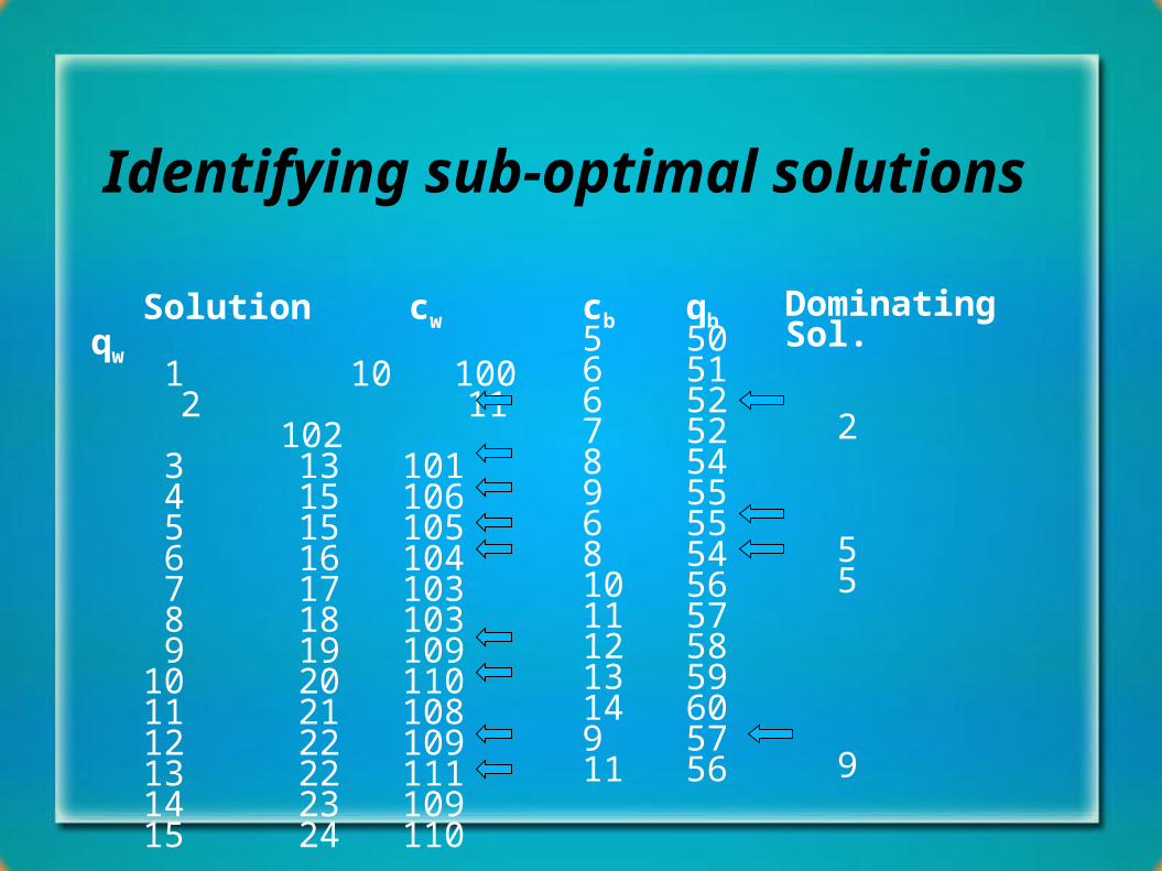
Identifying sub-optimal solutions

Solution cw qw 1 10 100 2 11

102 3 13 101 4 15 106 5 15 105 6 16 104 7 17 103 8 18 103 9 19 10910 20 11011 21 10812 22 10913 22 11114 23 10915 24 110

cb qb5 506 516 527 528 549 556 558 5410 5611 5712 5813 5914 609 5711 56

Dominating Sol.

2

55

9

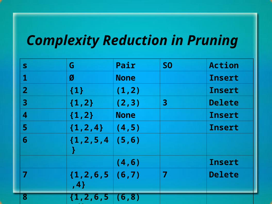
Complexity Reduction in Pruning

s G Pair SO Action

1 Ø None Insert

2 {1} (1,2) Insert

3 {1,2} (2,3) 3 Delete

4 {1,2} None Insert

5 {1,2,4} (4,5) Insert

6 {1,2,5,4} (5,6)

(4,6) Insert

7 {1,2,6,5,4} (6,7) 7 Delete

8 {1,2,6,5,4} (6,8)

(5,8) 8 Delete

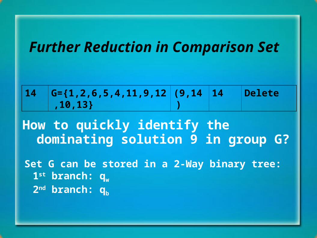
Further Reduction in Comparison Set

Set G can be stored in a 2-Way binary tree:1st branch: qw

2nd branch: qb

14 G={1,2,6,5,4,11,9,12,10,13} (9,14) 14 Delete

How to quickly identify the dominating solution 9 in group G?

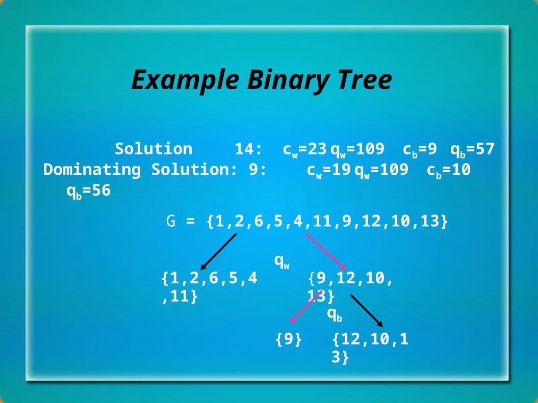
Example Binary Tree

Solution 14: cw=23 qw=109 cb=9 qb=57Dominating Solution: 9: cw=19 qw=109 cb=10 qb=56

G = {1,2,6,5,4,11,9,12,10,13}

{1,2,6,5,4,11} {9,12,10,13}qw

{9} {12,10,13}

qb

Outline

Motivation

Modelling late & early modes concurrently

Identifying sub-optimal solutions in a list

The merging problem

Power-Delay Trade-Off

Interaction between late & early modes (examples)

Conclusions, limitations and future directions

Acknowledgements

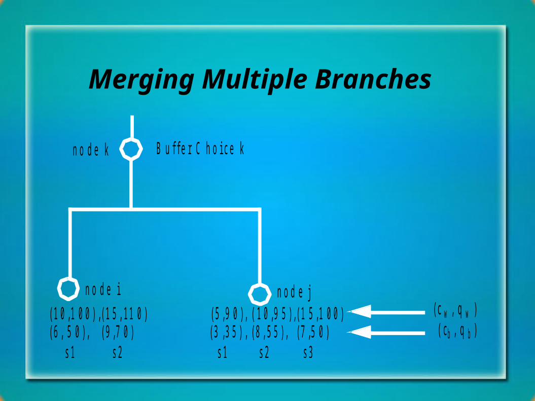
Merging Multiple Branches

Buffer Choice k

node i node j

node k

(10,100),(15,110) (5,90), (10,95),(15,100)

(6, 50), (9,70) (3,35), (8,55), (7,50)(cw , qw )(cb , qb )

s1 s2 s1 s2 s3

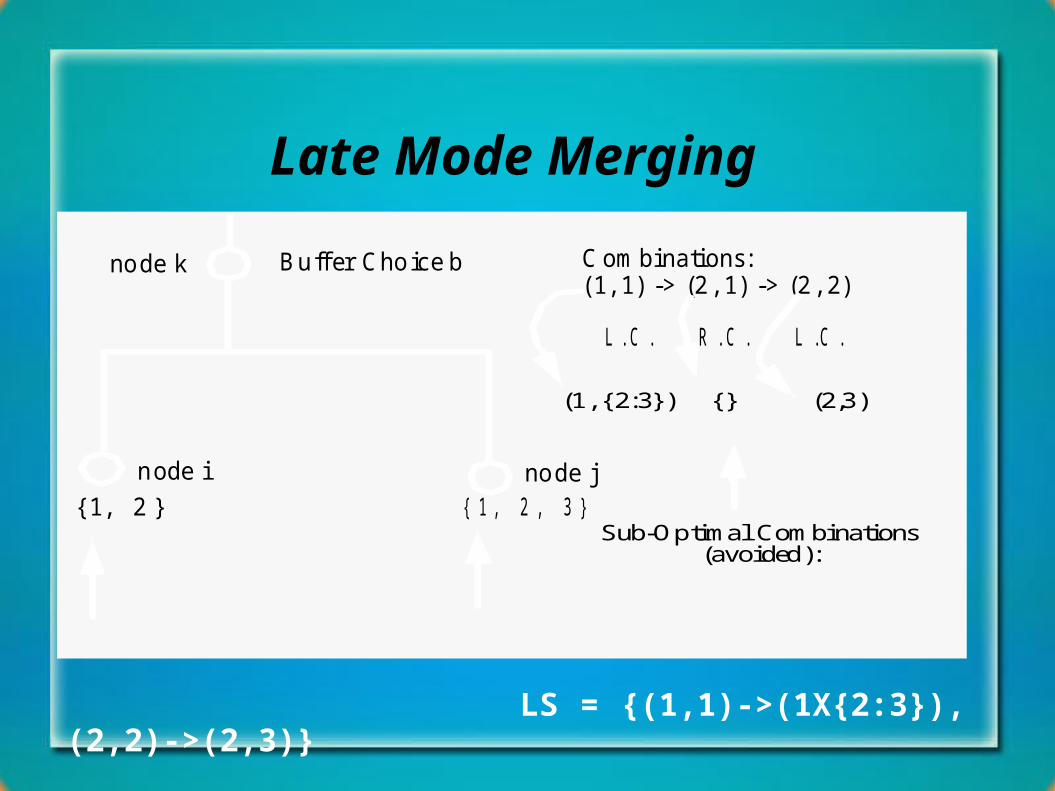
Late Mode Merging

LS = {(1,1)->(1X{2:3}), (2,2)->(2,3)}

Buffer Choice b

node i node j

node k

{1, 2 } {1, 2, 3}

Combinations:(1, 1) -> (2, 1) -> (2, 2) L.C. R.C. L.C.

Sub-Optimal Combinations(avoided):

(1, {2:3}) {} (2,3)

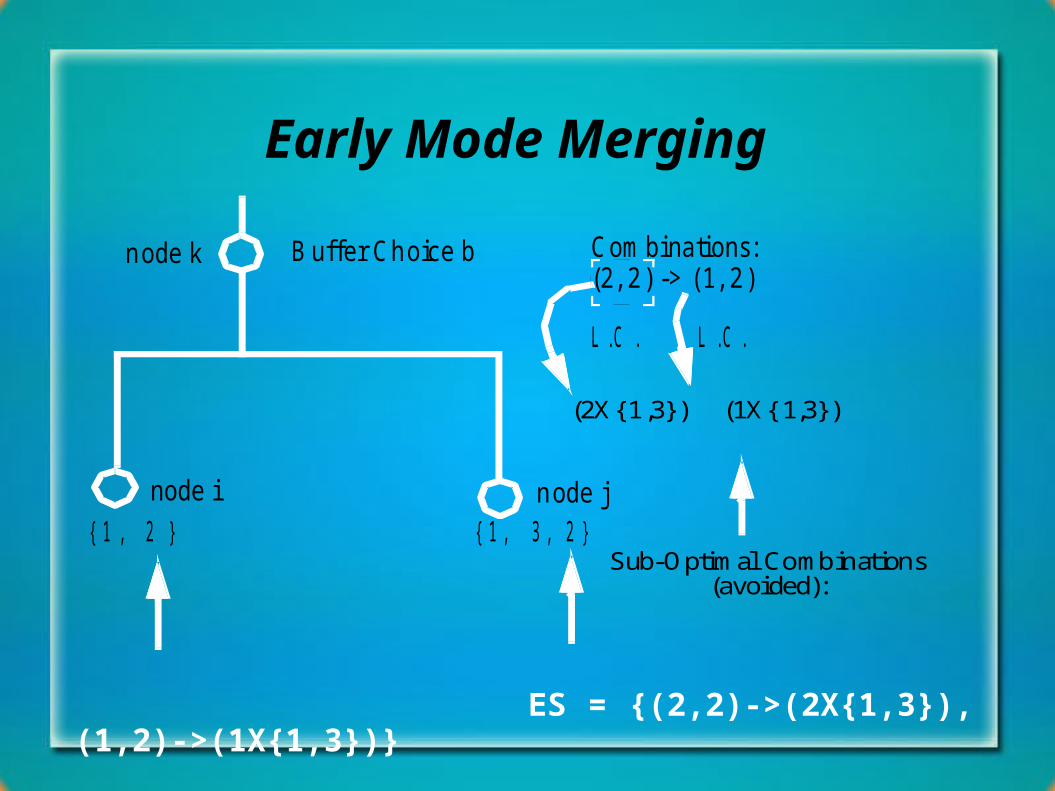
Early Mode Merging

Buffer Choice b

node i node j

node k

{1, 2 } {1, 3, 2}

Combinations:(2, 2) -> (1, 2) L.C. L.C.

Sub-Optimal Combinations(avoided):

(2X{1,3}) (1X{1,3})

ES = {(2,2)->(2X{1,3}), (1,2)->(1X{1,3})}

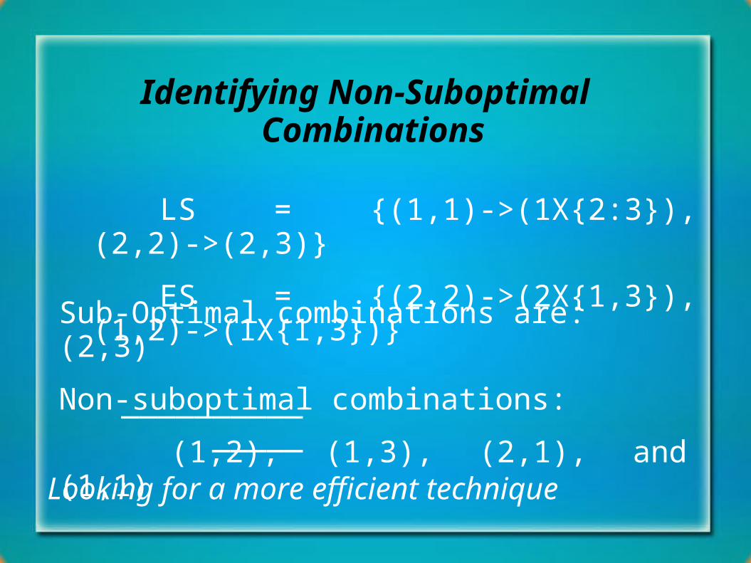
Identifying Non-Suboptimal Combinations

LS = {(1,1)->(1X{2:3}), (2,2)->(2,3)}

ES = {(2,2)->(2X{1,3}), (1,2)->(1X{1,3})}

Sub-Optimal combinations are: (2,3)

Non-suboptimal combinations:

(1,2), (1,3), (2,1), and (1,1)

Looking for a more efficient technique

__________ _____

Outline

Motivation

Modelling late & early modes concurrently

Identifying sub-optimal solutions in a list

The merging problem

Power-Delay Trade-Off

Interaction between late & early modes (examples)

Conclusions, limitations and future directions

Acknowledgements

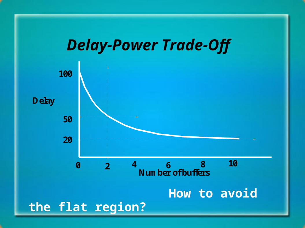
Delay-Power Trade-Off

2 4 6 8 10

100

50

20

0

Delay

Number of buffers

How to avoid the flat region?

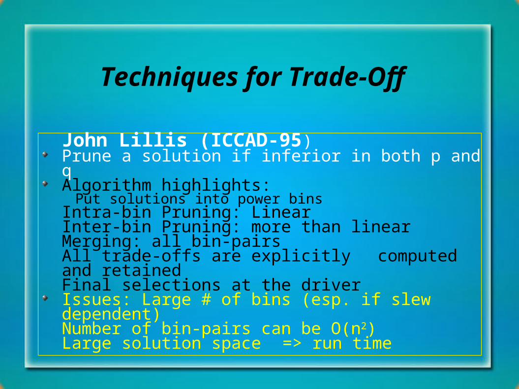
Techniques for Trade-Off

John Lillis (ICCAD-95)Prune a solution if inferior in both p and qAlgorithm highlights:

Put solutions into power binsIntra-bin Pruning: LinearInter-bin Pruning: more than linearMerging: all bin-pairsAll trade-offs are explicitly

computed and retainedFinal selections at the driver

Issues: Large # of bins (esp. if slew dependent)Number of bin-pairs can be O(n2)Large solution space => run time

Implicit Power-Delay Trade-Off

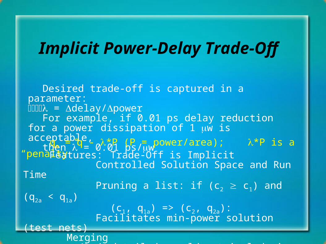
Desired trade-off is captured in a parameter: = delay/power

For example, if 0.01 ps delay reduction for a power dissipation of 1 w is acceptable,

then = 0.01 ps/w

qa = q - *P (P = power/area); *P is a “penalty” Features: Trade-Off is Implicit

Controlled Solution Space and Run TimePruning a list: if (c2 c1) and (q2a < q1a)

(c1, q1a) => (c2, q2a): Facilitates min-power solution (test nets)

MergingMuch detailed: could not include in this paper

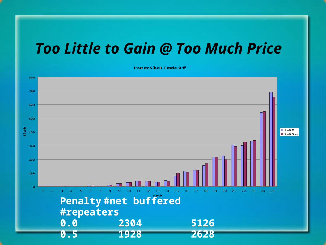
Too Little to Gain @ Too Much Price

Penalty #net buffered #repeaters0.0 2304 51260.5 1928 2628

Power-Slack Trade-Off

0

100

200

300

400

500

600

700

800

1 2 3 4 5 6 7 8 9 10 11 12 13 14 15 16 17 18 19 20 21 22 23 24 25

Slack

#P

ath

s

P=0.0

P=0.5ps

Outline

Motivation

Modelling late & early modes concurrently

Identifying sub-optimal solutions in a list

The merging problem

Power-Delay Trade-Off

Interaction between late & early modes (examples)

Conclusions, limitations and future directions

Acknowledgements

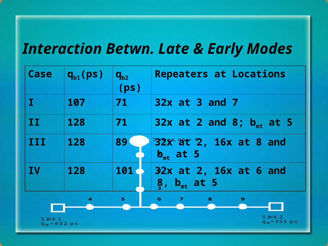
Interaction Betwn. Late & Early Modes

Case qb1(ps) qb2 (ps) Repeaters at Locations

I 107 71 32x at 3 and 7

II 128 71 32x at 2 and 8; bmt at 5

III 128 89 32x at 2, 16x at 8 and bmt at 5

IV 128 101 32x at 2, 16x at 6 and 8, bmt at 5

Sink 1 Sink 2

qw=632 ps qw=355 ps

Driver, qb = 0

1

2

3

4 5 6 7 8 9

Conclusion & Future Directions

A new model for repeater insertion problemEarly-mode timing requirement is a constraint

Helps avoid aggressive late-mode optimization creating new early mode violations

Should speed up design turn-around time by avoiding ECO’s to satisfy early-mode violations

Techniques forsatisfying maximum and minimum slew values, accurate timing to consider these slew values

and avoid the flat region in the power-delay curve

Limitations & Future Directions

LimitationsRun time complexitySlack Budgeting

Future research topics include:Combine gate sizing and repeater insertionCone basedGraph basedBetter merging techniquesControlling variations:

process, voltage and temperatureHierarchicalWe welcome collaboration with academia

Acknowledgements

Reviewers for detailed feedbackRob Mains for review & encouragementsAman Joshi and Sun Management for supportProgram Committee and the Organizers

Thank You

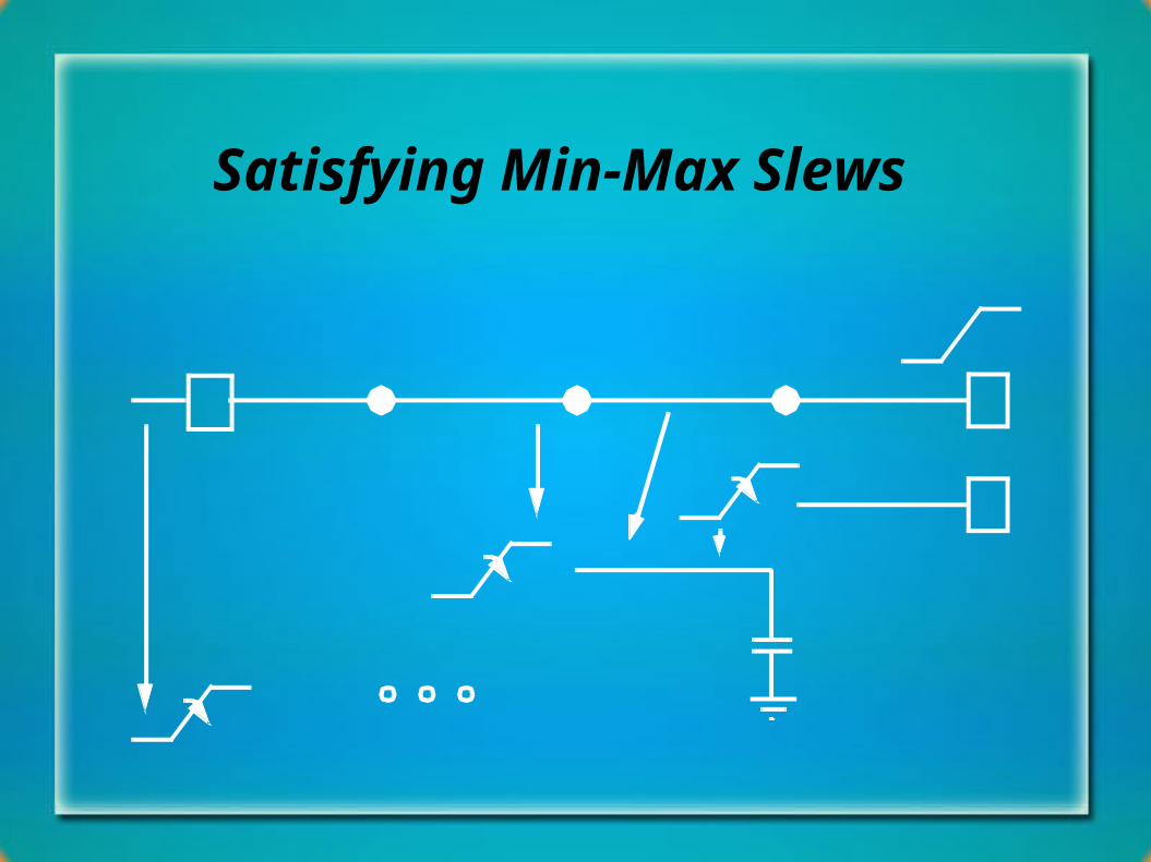
Satisfying Min-Max Slews