Isoprene derived secondary organic aerosol in a global ...€¦ · Isoprene derived secondary organic aerosol in a global aerosol chemistry climate model ... which was further studied

Isoprene derived secondary organic aerosol in a global aerosolchemistry climate modelScarlet Stadtler1, Thomas Kühn2,3, Sabine Schröder1, Domenico Taraborrelli1, Martin G. Schultz1,*, andHarri Kokkola2

1Institut für Energie- und Klimaforschung, IEK-8, Forschungszentrum Jülich, Germany2Finnish Meteorological Institute, P.O. Box 1627, 70211, Kuopio, Finland3Department of Applied Physics, University of Eastern Finland, P.O. Box 1627, 70211, Kuopio, Finland*Now at Jülich Supercomputing Centre, JSC, Forschungszentrum Jülich, Germany

Correspondence to: Harri Kokkola ([email protected])

Abstract

Within the framework of the global chemistry climate model ECHAM-HAMMOZ a novel explicit coupling between the

sectional aerosol model HAM-SALSA and the chemistry model MOZ was established to form isoprene derived secondary

organic aerosol (iSOA). Isoprene oxidation in the chemistry model MOZ is described by a semi-explicit scheme consisting of

147 reactions, embedded in a detailed atmospheric chemical mechanism with a total of 779 reactions. Low volatile compounds5

(LVOC) produced during isoprene photooxidation are identified and explicitly partitioned by HAM-SALSA. A group contri-

bution method was used to estimate their evaporation enthalpies and corresponding saturation vapor pressures, which are used

by HAM-SALSA to calculate the saturation concentration of each LVOC. With this method, every single precursor is tracked

in terms of condensation and evaporation in each aerosol size bin. This approach lead to the identification of ISOP(OOH)2 as

a main contributor to iSOA formation. Further, reactive uptake of isoprene epoxidiols (IEPOX) and isoprene derived glyoxal10

were included as iSOA sources. The parameterization of IEPOX reactive uptake includes a dependency on aerosol pH value.

This model framework connecting semi-explicit isoprene oxidation with explicit treatment of aerosol tracers leads to a global,

annual isoprene SOA yield of 16% relative to the primary oxidation of isoprene by OH, NO3, and ozone. With 445 Tg (392

TgC) isoprene emitted, an iSOA source of 148 Tg (61 TgC) is simulated. The major part of iSOA in ECHAM-HAMMOZ is

produced by IEPOX (24.4 TgC) and ISOP(OOH)2 (28.3 TgC). The main sink process is particle wet deposition which removes15

143 Tg (59 TgC). The iSOA burden reaches 1.6 Tg (0.7 TgC) in the year 2012.

1 Introduction

Atmospheric particles play an important role in the earth system, especially in the interactions between climate (IPCC, 2013)

and human health (Fröhlich-Nowoisky et al., 2016; Lakey et al., 2016). Aerosols interact with atmospheric radiation directly

via absorption and scattering, and indirectly via cloud formation. These interactions depend on the particles’ microphysical20

1

Geosci. Model Dev. Discuss., https://doi.org/10.5194/gmd-2017-244Manuscript under review for journal Geosci. Model Dev.Discussion started: 16 October 2017c© Author(s) 2017. CC BY 4.0 License.

properties, their chemical composition and phase state (Ghan and Schwartz, 2007; Shiraiwa et al., 2017). In the current political

debates about air quality and climate change, understanding atmospheric particles is one of the most challenging problems and

led to increased research in this field over the last two decades (Fuzzi et al., 2015). Especially organic aerosols are not well

understood and subject of ongoing research (Pandis et al., 1992; Kanakidou et al., 2005; Zhang et al., 2007; Fuzzi et al., 2015;

Hodzic et al., 2016). Organic aerosol (OA) consists of two types of particles, often mixed and difficult to distinguish (Kavouras5

et al., 1999; Donahue et al., 2009). First, organic aerosol can be emitted directly into the atmosphere as primary organic aerosol

(POA) (Kanakidou et al., 2005; Dentener et al., 2006). Second, organic aerosol mass is also formed from organic gases which

are emitted as volatile organic compounds (VOC) and transformed into compounds capable of partitioning into the particle

phase. This second type of organic aerosol is called secondary organic aerosol (SOA) (Pankow, 1994; Seinfeld and Pankow,

2003; Jimenez et al., 2009). Both types of organic aerosols are challenging to model due to limited knowledge about emissions,10

composition, evolution and physicochemical properties (Lin et al., 2012). Concerning SOA, there are additional uncertainties

concerning SOA precursors and the atmospheric chemistry leading to their formation (Heald et al., 2005). Up to now, global

models have lacked an explicit treatment of SOA (Zhang et al., 2007) and use relatively simple parameterisations to form

SOA, for example with the two-product model based on Odum et al. (1996). Such parameterisations neglect explicit chemical

transformation and assume fixed SOA yields based on laboratory studies (Tsigaridis and Kanakidou, 2003; ODonnell et al.,15

2011). Donahue et al. (2006) presented with their volatility basis set (VBS) another approach that allows to distinguish between

various precursor VOC, but still does not consider explicit chemical formation and molecular identity of the compounds. The

VBS system was further developed to include aerosol aging based on observations of O:C ratio (Donahue et al., 2011). Lin

et al. (2012) and Marais et al. (2016) made first steps into coupling explicit formation of SOA precursors with SOA formation,

focusing on specific compounds.20

Global models largely underestimate the amount of atmospheric organic aerosol (Volkamer et al., 2006; De Gouw and

Jimenez, 2009; Tsigaridis et al., 2014). This underestimation might be related to the huge number of organic compounds in

the atmosphere (Goldstein and Galbally, 2007) which cannot be identified individually by state-of-the-art measuring devices.

For explicit modeling it is necessary to characterize their chemical properties, structures, volatility, solubility and further

reactions pathways in the particle phase. Donahue et al. (2009) argues that it is extremely difficult to accomplish dissecting this25

complexity in detail.

This study makes an attempt to explore the influence of a semi-explicit chemical mechanism implementing a state-of-the-art

isoprene oxidation that is based on Taraborrelli et al. (2009, 2012); Nölscher et al. (2014); Lelieveld et al. (2016) on isoprene

derived secondary organic aerosol (iSOA) formation. Recently, isoprene was identified to contribute to SOA. Literature iSOA

yields vary between 1% and 30% relative to the total amount of isoprene oxidized by OH, O3, and NO3 (Surratt et al., 2010).30

Even with a yield as low as 1%, isoprene as a source of SOA has a huge impact, since global annual isoprene emissions

are estimated to range between 500 and 750 Tg a−1 (Guenther et al., 2006). Therefore, iSOA was investigated in field and

laboratory experiments (Claeys et al., 2004; Surratt et al., 2006, 2007a, b). These studies could identify isoprene derived

compounds in the particle phase and identified possible formation pathways (Liggio et al., 2005a; Lin et al., 2013b; Berndt

2


et al., 2016; DAmbro et al., 2017a). First generation products of isoprene are too volatile to partition into the the aerosol phase

(Kroll et al., 2006), however they contribute significantly to iSOA formation via heterogeneous and multiphase reactions.

Glyoxal and isoprene epoxide (IEPOX) were identified to undergo reactive uptake and subsequent aqueous-phase reactions

(Liggio et al., 2005b; Paulot et al., 2009). Glyoxal uptake might be followed by oligomerization and organo-sulfate formation

depending on aerosol pH value, which is considered to be an irreversible uptake (Liggio et al., 2005a, b). Therefore, glyoxal5

derived SOA was studied in different model configurations with reversible and irreversible uptake (Volkamer et al., 2007; Fu

et al., 2008; Ervens and Volkamer, 2010; Washenfelder et al., 2011; Waxman et al., 2013; Li et al., 2013).

Experimental and ambient measurements found 2-methyltetrol in the particle phase, which is attributed to be formed by

IEPOX (Claeys et al., 2004; Paulot et al., 2009; Surratt et al., 2006). Therefore, irreversible reactive uptake from IEPOX was

proposed. Surratt et al. (2007b) studied the effect of pH value on iSOA and found organic carbon to be a function of aerosol pH10

which was further studied leading to the reaction mechanism for 2-methyltetrol formation from IEPOX to be an acid catalyzed

ring opening reaction (Eddingsaas et al., 2010; Lin et al., 2013a) and was used to create process parametrizations (Pye et al.,

2013; Riedel et al., 2015). Nevertheless, IEPOX uptake was mostly studied in experiments using sulfate aerosol seeds to explore

IEPOX uptake dependence on aerosol pH, which leads to the question whether the reaction might be sulfate catalyzed instead

(Surratt et al., 2007a; Xu et al., 2015). However, non-racemic mixtures of tetrols stereoisomers in the atmosphere point to a15

substantial biological origin (Nozière et al., 2011).

After exploring the IEPOX iSOA formation pathway, experimental studies could also identify non-IEPOX iSOA formation

pathways via the highly oxidized, very low volatile isoprene product dihydoxy dihyodroperoxide (C5H12O6, ISOP(OOH)2)

(Riva et al., 2016; Liu et al., 2016; Berndt et al., 2016; DAmbro et al., 2017a). This compound was identified under low NOx,

meaning HO2 dominated conditions (Berndt et al., 2016) and neutral aerosol pH (Liu et al., 2016; DAmbro et al., 2017a).20

In the light of the available knowledge on iSOA formation, this study focuses on iSOA formation via reactive uptake and

explicit partitioning of exclusively low volatile isoprene derived compounds. This paper is organized as follows: Section 2

describes the model framework including the sub-models ECHAM6, HAM-SALSA and MOZ. This includes a detailed de-

scription of the selection procedure for iSOA precursors and the interplay between the gas-phase oxidation of these and the

SALSA aerosol scheme. Furthermore, Section 2 describes the model setup and sensitivity runs performed. Section 3 shows25

the simulation results of the reference run including all iSOA formation pathways, e.g. global annual budget and mean surface

concentrations. Furthermore, it discusses sensitivity runs and model uncertainties for formulation of the reactive uptake of

IEPOX and the impacts of evaporation enthalpy. Section 4 discusses possible error sources according to used parametrizations

and assumptions and 5 provides conclusions.

2 Method30

2.1 Model description

For this study the aerosol chemistry climate model ECHAM-HAMMOZ in its version ECHAM6.3-HAM2.3MOZ1.0 is used

(https://redmine.hammoz.ethz.ch/projects/hammoz/wiki/Echam630-ham23-moz10), Schultz et al. (submitted)). This model

3


framework consists of three coupled models. ECHAM6 is the sixth generation climate model which evolved from the European

Center for Medium Range Weather Forecasts (ECMWF) developed in the Max Planck Institute for Meteorology (Stevens et al.,

2013). In order to simulate climate, ECHAM6 solves the prognostic equations for vorticity, divergence, surface pressure and

temperature expressed as spherical harmonics with triangular truncation (Stier et al., 2005). All tracers are transported with a

semi Lagrangian scheme on a Gaussian grid (Lin and Rood, 1996). Hybrid σ-pressure coordinates with a pressure range from5

1013 hPa to 0.01 hPa are used for vertical discretization. Aerosol tracers are simulated by the Hamburg Aerosol Model HAM

with aerosol microphysics based on the Sectional Aerosol module for Large Scale Applications SALSA (Kokkola et al., 2008;

Bergman et al., 2012). In addition, the chemistry model MOZ simulates atmospheric concentrations of trace gases interacting

with aerosols and climate system (Stein et al., 2012). A detailed description of the HAMMOZ model system is given in Schultz

et al. (submitted).10

For this study SALSA is extended to partition organic trace gases simulated by MOZ between the gas and aerosol phases.

Additionally, the isoprene oxidation scheme in the MOZ chemical mechanism was modified in order to model secondary

organic aerosol formation. Details can be found in Sections 2.1.1 and 2.1.2.

Aerosol and trace gas emissions are taken from the ACCMIP interpolated emission inventory (Lamarque et al., 2010).

Interactive gas phase emissions of VOC are simulated by MEGAN (Model of Emissions of Gases and Aerosols from Nature)15

(Guenther et al., 2006). For details about the implementation of MEGAN v2.1 in ECHAM-HAMMOZ and its evaluation it is

referred to Henrot et al. (2017).

For all simulations the triangular truncation 63, leading to horizontal resolution of 1.875◦× 1.875 ◦and 47 vertical layers is

used. The lowest layer, corresponding to the surface layer, thickness is around 50 m.

2.1.1 Chemistry model MOZ20

Atmospheric chemistry is simulated by MOZ solving the chemical equations using an implicit Euler backward solver and treat-

ing emissions, dry and wet deposition. The current MOZ version evolved from an extensive atmospheric chemical mechanism

based on MOZART version 3.5 (Model for Ozone and Related chemical Tracers) (Stein et al., 2012), which merges the tro-

pospheric version MOZART-4 (Emmons et al., 2010) with the stratospheric version MOZART-3 (Kinnison et al., 2007). The

chemical mechanism was further developed including a detailed isoprene oxidation scheme based on Taraborrelli et al. (2009,25

2012); Nölscher et al. (2014); Lelieveld et al. (2016) with revised peroxy radical chemistry (Schultz et al., submitted), lead-

ing to a model system resembling the CAM-chem model (Community Atmosphere Model with Chemistry) (Lamarque et al.,

2010). The chemical mechanism version used here is called JAM3 (Jülich Atmospheric Mechanism version 3). It differs from

version 2 of this mechanism in self and cross reactions of isoprene products, added nitrates, initial reactions for monoterpenes

and sesquiterepenes and production of very low volatile highly oxidized molecules. The additional isoprene related reactions30

can be found in Table S1. Similar extensions of terpenes oxidation are planned; the current study focuses on isoprene. In total

254 gas species are undergoing 779 chemical reactions including 146 photolysis, 16 stratospheric heterogeneous and 8 tropo-

spheric heterogeneous reactions. The semi-explicit isoprene oxidation with 147 reactions constitutes a major of these reactions

in JAM3.

4


Compound SMILES code p∗0(298.15K) [Pa] ∆Hvap [ kJmol

] H [moleatm

]

LNISOOH O=CC(O)C(C)(OO)CON(=O)=O* 2.2 · 10−4 122.7 2.1 · 105

CC(O)(CON(=O)=O)C(OO)C=O 3.8 · 10−4 120.0

LISOPOOHOOH OC(C)(COO)C(CO)OO* 3.8 · 10−7 155.3 2.0 · 1016

CC(CO)(C(COO)O)OO 1.9 · 10−7 158.9

LC578OOH OCC(O)C(C)(OO)C=O* 2.0 · 10−4 123.2 3.0 · 1011

O=CC(O)C(C)(CO)OO 2.0 · 10−4 123.2

C59OOH OCC(=O)C(C)(CO)OO* 1.0 · 10−4 125.0 3.0 · 1011

Table 1. Isoprene oxidation products in JAM3, physical characteristics and molecular structure expressed as SMILES code. Saturation

vapor pressure at the reference temperature 298 K p∗0, Henry’s law coefficient H and evaporation enthalpy ∆Hvap. ∆Hvap and p∗0 are

used in Clausius Clapeyron equation for calculation of the saturation vapor pressure as a function of temperature in SALSA. Names of the

compounds rely on the Master Chemical Mechanism (MCM 3.2), except for LISOPOOHOOH, which is not in MCM 3.2. Names starting

with "L" indicate that this specie is lumped, SMILES codes of all isomers are shown, but just the ones marked with * are used.

In order to identify SOA precursors produced via isoprene oxidation, first, for each specie a molecular structure was assigned.

Some species are not represented explicitly, but instead they represent groups of compounds with similar chemical properties

(lumping). In these cases a group of isomers were assigned to one structure. These structures are expressed as SMILES codes

in Table 1 and as chemical structures in Figure 1. With those molecular structures, second, the saturation vapor pressure p∗(T )

of each organic compound in JAM3 was estimated using the group contribution method by Nannoolal et al. (2008) and the5

boiling point method by Nannoolal et al. (2004) in the framework of the online open source facility UManSysProp (Topping

et al., 2016). Third, the group contribution method data was fitted to the Clausius Clapeyron equation in order to determine the

evaporation enthalpy ∆Hvap for each compound. Finally, those species with saturation vapor pressures p∗0 at 298.15 K lower

than 0.01 Pa were classified as low volatility compounds. This procedure leads to four low volatile isoprene oxidation products

contributing to iSOA in ECHAM-HAMMOZ. Table 1 gives the SMILES codes and resulting saturation vapor pressure at10

the reference temperature p∗0 and the evaporation enthalpy ∆Hvap for all low volatile iSOA precursors. The uncertainties in

structure assignment of lumped species and the sensitivity to ∆Hvap are explored in Sections 3.2.3 and 3.3.

Figure 1 shows the chemical pathways of isoprene oxidation and their products to form LIEPOX, LNISOOH, LISOPOOH-

OOH, LC578OOH and C59OOH. For the whole chemical mechanism including IGLYOXAL formation, it is referred to the

model description of HAMMOZ in Schultz et al. (submitted).15

Low volatile isoprene oxidation products are formed in MOZ via several reaction steps. Four of these LVOCs were identified

and their formation is based on two initial reaction pathways from the oxidation of isoprene by OH and NO3 respectively. Also

the O3 initiated reactions pathways are included in MOZ, but none of the products was low volatile enough. The OH initiated

pathway leads to three LVOCs called C59OOH, LC578OOH and LISOPOOHOOH in our mechanism. First, OH attacks

isoprene C5H8 and forms three isoprene peroxy radical isomers, where one of them is a lumped specie. For simplicity there are20

5


called here ISOPO2.

C5H8 + OH→ ISOPO2 (R1)

ISOPO2 undergoes reactions with ambient radicals, but also self and cross reactions leading alcohols (ISOPOH), isoprene

hydroperoxides (ISOPOOH) and isoprene nitrates (ISOPNO3).

ISOPO2 seeText→ ISOPOH + ISOPOOH + ISOPNO3 (R2)5

From the reactions of ISOPOH and ISOPOOH with OH a hydroperoxide peroxy radical is formed, a lumped specie called

LISOPOOHO2, which can be oxidized by HO2 or CH3O2 to LISOPOOHOOH. Not included is the H-shift of LISOPOOHO2

that yields much more volatile compounds than LISOPOOHOOH (DAmbro et al., 2017b), so the chemical yield of LISOPOOH-

OOH is expected to be an upper estimate. LISOPOOHOOH has the highest yield of the LVOC considered here, 9% of

isoprene end up as LISOPOOHOOH.10

ISOPOH + OH → LISOPOOHO2 + LIEPOX (R3)

ISOPOOH + OH → LISOPOOHO2 (R4)

LISOPOOHO2 + HO2 → LISOPOOHOOH (R5)

LISOPOOHO2 + CH3O2 → LISOPOOHOOH (R6)

LISOPOOHOOH can either react back to LISOPOOHO2, be photolysed or oxidized by OH to form LC578OOH.15

LISOPOOHOOH + OH→ LC578OOH (R7)

LC578OOH is another LVOC, which is more volatile than LISPOOHOOH and can be formed also via another pathway

starting from ISOPO2, ISOPOOH and ISOPNO3, which either react with radicals, or in the case of the nitrate are photolysed

leading to LHC4CCHO, which then reacts with OH to LC578O2. Finally, LC578O2 reacts with HO2 and forms LC578OOH,

which either can react back to LC578O2 with OH or be photolysed. Just 1% of the oxidation of isoprene leads to LC578OOH.20

ISOPO2 + RO2 → LHC4CCHO (R8)

ISOPOOH + NO → LHC4CCHO (R9)

ISOPNO3 +hν → LHC4CCHO (R10)

LHC4CCHO + OH → LC578O2 (R11)

LC578O2 + HO2 → LC578OOH (R12)25

The third compound formed from the OH initiated oxidation of isoprene is C59OOH. Starting from ISOPO2, there are two

possible oxidation ways for C59OOH formation, one with nitrates as intermediates and a second one where nitrogen oxide is

not required. The nitrate pathway starts with formation of ISOPNO3 from ISOPO2 and continues with OH reaction to form

6


isoprene nitrate peroxy radicals ISOPNO3O2, which is again a lumped specie.

ISOPNO3 + OH → ISOPNO3O2 (R13)

ISOPNO3O2 + CH3O2 → ISOPNO3OOH (R14)

ISOPNO3OOH + OH → C59OOH (R15)

Via formation of a nitrate hydoxyperoxy radical, finally C59OOH is formed. This pathway requires the availability of NO. For5

the second pathway, no NO is needed.

ISOPO2 + ISOPO2 → HCOC5 (R16)

HCOC5 + OH → C59O2 (R17)

C59O2 + HO2 → C59OOH (R18)

Self-reactions of ISOPO2 lead to formation of HCOC5, which is then converted via OH to C59O2. HO2 oxididses C59O2 to10

C59OOH. C59OOH can also react back to C59O2 or be lost via photolysis. The overall yield from isoprene to C59OOH is

2%.

The fourth LVOC is an isoprene derived nitrate LNISOOH, which requires both, a NOx dominated and a HO2 dominated

environment, because only the first two oxidation steps use nitrate, then OH and HO2 are required. First, isoprene reacts with

NO3 radical and forms a nitrate peroxy radical NIOSPO2, which oxidizes NO and forms NC4CHO. NC4CHO in contrast,15

has to react with OH to form LNISO3, which then reacts with HO2 and forms LINSOOH.

C5H8 + NO3 → NISOPO2 (R19)

NISOPO2 + NO → NC4CHO (R20)

NC4CHO + OH → LNISO3 (R21)

LNISO3 → LNISOOH (R22)20

LNISOOH can be photolysed or react back to LNISO3. Due to the requirements of both NO and HO2 to be present, formation

of LINSOOH is limited and this compound is only generated with a very low yield of just 0.1% from isoprene oxidation.

In Figure 1 the simplified overview over the described chemical reactions can be found. Reaction branching ratios from

isoprene to the final compounds are shown as chemical structures used for the LVOCs. In the particle phase, the fraction which

ends up in the iSOA is expressed as percentage of total produced by partitioning LVOC and reactive uptake.25

To cover multiphase chemical iSOA formation, heterogeneous reactions on aerosols of IEPOX and isoprene derived glyoxal

were included. Nevertheless, ECHAM-HAMMOZ does not include in-particle or in-cloud aqueous phase chemistry, therefore

no assumptions of in-particle products are made. Furthermore, no SOA formation via cloud droplets is included in ECHAM-

HAMMOZ due to constraints in the aerosol cloud interaction formulation. Therefore, reactive uptake is parameterized as

pseudo first order loss using aerosol surface area density given by HAM, according to Schwartz (1986) and described in detail30

in Stadtler et al. (2017).

7


Figure 1. Simplified overview over chemical pathways leading to low volatile isoprene derived compounds able to partition into aerosol

phase. Note that ISOPO2 here is used for simplicity, JAM3 includes three different ISOPO2 (LISOPACO2, ISOPBO2, ISOPDO2), same

applies for ISOPOH and ISOPOOH. The percentages in the boxes indicate reaction turnover of isoprene leading to these products. For

IGLYOXAL there are too many formation pathways and are therefore not shown. The solid horizontal curve represents the boundary to the

particle phase. Percentages found under the corresponding arrow express the individual iSOA yield of the compound. Except for LIEPOX

and IGLYOXAL, structures are relevant to estimate the saturation vapor pressure and evaporation enthalpy and are therefore shown here.

For the detailed mechanism it is referred to Schultz et al. (submitted).

8


In MOZ, three IEPOX isomers are lumped together (LIEPOX) and a compound IGLYOXAL was introduced to be able

to differentiate between isoprene derived glyoxal and glyoxal from other sources. Isoprene glyoxal formation pathways are

numerous and no changes were made to the mechanism with respect to IGLYOXAL formation. Since these reactions are

included also in JAM2, see Schultz et al. (submitted). LIEPOX is formed along the pathway described for LISPOOHOOH

in Reaction, see (R3).5

Glyoxal is observed to produce a variety of compounds, like oligomers or organosulfates, in the aqueous aerosol phase and

glyoxal is capable of be released back in the gas phase (Volkamer et al., 2007; Ervens and Volkamer, 2010; Washenfelder et al.,

2011; Li et al., 2013). The simplification assuming irreversible uptake might thus overestimate its impact on iSOA. Following

previous model studies (Fu et al., 2008; Lin et al., 2012) a reaction probability of γglyoxal = 2.9 · 10−3 (Liggio et al., 2005b) is

used.10

For IEPOX the irreversibility is a less critical assumption, because IEPOX forms 2-methyltetrol and organosulfates in the

aqueous aerosol phase, which stay in the aerosol phase (Claeys et al., 2004; Eddingsaas et al., 2010; Lal et al., 2012; McNeill

et al., 2012; Woo and McNeill, 2015). However, ECHAM-HAMMOZ does not include explicit treatment of aqueous phase

reactions. The reaction probability of IEPOX varies with pH value (Lin et al., 2013a; Pye et al., 2013; Gaston et al., 2014)

which cannot be captured by HAMMOZ due to the lack of ammonium and nitrate in the aerosol phase, thus the possibility to15

capture aerosol pH. For these reasons, the reaction probability of IEPOX γIEPOX = 1 · 10−3 (Gaston et al., 2014) was chosen,

close to the value used by (Pye et al., 2013). To explore the impact of the pH dependence sensitivity runs with different γIEPOX

are analyzed. Additionally, no assumptions of in-particle products are made, in ECHAM-HAMMOZ IEPOX is simply taken

up into aerosol phase without further transformation.

2.1.2 HAM-SALSA20

The Hamburg Aerosol Model (HAM) handles the evolution of atmospheric particles and includes emissions, removal, micro-

physics and radiative effects. Moreover, the current configuration uses the Sectional Aerosol module for Large Scale Applica-

tions (SALSA) for calculation of aerosol microphysics (Kokkola et al., 2008). In SALSA the aerosol size distribution is divided

into aerosol size sections (size bins). Furthermore, these size bins are grouped into sub-ranges, which allows the model to limit

the computation of the aerosol microphysical processes to only the aerosol sized that are relevant to these processes. Micro-25

physical processes simulated by SALSA cover nucleation, condensation, coagulation, cloud activation, sulfate production and

hydration (Bergman et al., 2012). The aerosol composition is described using five different aerosol compounds, sulphate, black

carbon, dust, sea salt and organic carbon. Furthermore, SALSA treats secondary organic aerosol formation via the volatility

basis set (Kühn et al., in preparation). In the model setup described there, SALSA uses a strongly simplified description for

VOC oxidation (pseudo chemistry) to obtain SOA precursors. Here this model system was extended and coupled to MOZ,30

which explicitly calculates SOA precursors as described in Section 2.1.1. The standard SALSA-VBS system is not used here.

Instead for each SOA-forming compound the gas-to-particle partitioning is treated explicitly and its concentration is tracked

in both the gas and the aerosol phases separately. This study exclusively uses isoprene-derived precursors to form iSOA, other

oxygenated compounds capable of partitioning derived from terpenes or aromatics are neglected.

9


2.1.3 Coupling of HAM-SALSA and MOZ

HAM-SALSA and MOZ interact though several processes, oxidation fields calculated by MOZ are passed to HAM-SALSA

for aerosol oxidation, MOZ produces H2SO4 which is then converted by HAM-SALSA to sulphate aerosol and HAM-SALSA

provides the aerosol surface area density for heterogeneous chemistry. Above all, HAM-SALSA takes the information of iSOA

precursor gas phase concentrations and their physical properties to calculate the saturation concentration coefficient (C∗) using5

Clausius Clapeyron equation (1) (Farina et al., 2010).

C∗i = C∗i (T0)T0

Texp

[∆Hvap

R

(1T0− 1T

)](1)

Here T0 is the reference temperature of 298.15 K and ∆Hvap is the evaporation enthalpy given in Table 1 for the iSOA

precursors identified in this study. C∗ is then used to calculate the explicit partitioning of the iSOA precursors to each aerosol

section. This process is reversible and it is thus possible that the iSOA formed in one region is transported and evaporates in10

another region. Explicitly calculating the partitioning instead of prescribing yields in chemical production or SOA formation is

a key difference to other models with fixed yields. Loss processes for SOA in HAM-SALSA include sedimentation, deposition

and wash out in the aerosol phase.

2.2 Simulation set up and sensitivity runs

An overview of the performed simulations can be found in Table 2. The reference simulation RefBase, which includes a three-15

month spin up and spans the time from October 2011 until the end of December 2012, is evaluated for the entire year 2012,

while all other sensitivity runs are limited to the northern hemispheric, isoprene emission intense, summer season of June, July

and August.

Several sensitivity simulations were performed to explore model sensitivities and assess uncertainties. For comparison of

the explicit ECHAM-HAMMOZ scheme to a state-of-the-art VBS scheme, ECHAM-HAM whith pseudo chemistry and VBS20

configuration (RefVBS), described in 2.1.2, was run. ∆H30 uses the same, much lower evaporation enthalpy of ∆Hvap =

30 kJmol for all partitioning LVOC following Farina et al. (2010). Furthermore, pH value dependence of IEPOX is tested in

γIEX formulating an easy pH dependent parameterization based on laboratory measurements. Particle pH values cannot be

obtained from ECHAM-HAMMOZ itself as the model does not include the calculation of particle phase thermodynamics. For

this reason, aerosol pH was calculated offline using the AIM aerosol thermodynamics model (Clegg et al., 1998). The SALSA25

simulated annual mean mass of aerosol water and the mean mass of aerosol-phase inorganic compounds at the lowest model

level were used an input for AIM. This required two additional assumptions: (1) all aerosol is in liquid form, (2) all sulfate

is in form of ammonium bisulfate. This second assumption for sulfate has to be done, because particle phase ammonia is not

modeled in the current configuration of ECHAM-HAMMOZ. Using these inputs, AIM provided the concentration of hydrogen

ion (H+) as an output.30

10


Simulation Description

RefBase Reference run with uniform reaction probabilities for IEPOX and isoprene glyoxal

γIEPOX = 1.0 · 10−3, γIGY OXAL = 2.9 · 10−3 (see Section 2.1.1),

LVOC ∆Hvap and p∗0(298.15K) given in Table 1.

RefVBS VBS approach with pseudo chemistry.

∆H30 Run like reference run, but with same ∆Hvap = 30 kJmol

for all compounds.

γpH Like RefBase, but with γIEPOX = f(pH).Table 2. Description of simulations performed.

Figure 2. Reference run annual average surface distribution of precursor gases and iSOA in µg m−3 for 2012.

3 Results

3.1 Reference run RefBase

3.1.1 Global distributions

Figure 2 shows the annual mean surface concentrations for total iSOA and its precursors in the gas phase. The precursors

are formed, except for LNISOOH, during daytime and build up quickly. Therefore, these are found very close to isoprene5

source regions mostly in the tropics and southern hemisphere. Their highest values, up to 3 µg m−3, are simulated over the

Amazon, the east flank of the Andes, Central Africa, North Australia, Indonesia and Southeast Asia. In the annual mean also

the northern hemispheric summer is visible, but peak values of over 2 µg m−3 are only reached on Mexico’s west coast and in

the southeastern US. In Europe and North Asia, where isoprene emissions are much lower, mean values up to 0.5 µg m−3 of

precursors are formed.10

11


These low precursor concentrations correspond to the very low iSOA concentrations over Europe and North Asia, compared

to Southeastern US and Mexico’s west coast, where up to 4.5 µg m−3 iSOA is formed. The highest iSOA concentrations are

found where high precursor concentrations meet pre-existing aerosol, like in Central Africa because of it high biomass burning

emissions or Southeast Asia, where aerosol pollution is high. In the latter ECHAM-HAMMOZ simulates values of up to

13 µg m−3 if iSOA. The Amazon is a region of very high isoprene emissions and therefore high iSOA precursor concentrations,5

nevertheless the local maximum in iSOA of 14 µg m−3 can be seen on the east side of the Andes. This pattern is caused by

pre-existing aerosol, which in ECHAM-HAMMOZ tends to accumulate on the east side of the Andes, and the still high iSOA

precursor concentrations in the same region. Also in the norhtern part of Australia higher precursor loadings are found, leading

there to iSOA ground-level concentrations of up to 9 µg m−3.

It can also be seen, that iSOA has a longer lifetime than its gas-phase precursors. Prevailing wind directions are recognizable,10

clearly showing transport of iSOA over the oceans, for example in the South American and African outflow regions. Also,

iSOA is transported from Australia to the north. The average iSOA lifetime was calculated to be around 4 days, so long-range

transport is limited, before iSOA is lost due to wet deposition (see Section 3.1.2).

Farina et al. (2010) included iSOA formation with fixed yields of isoprene transformation to the different VBS classes and

also showed its global annual surface distribution for 1979 - 1980. Compared to Farina et al. (2010) ECHAM-HAMMOZ15

simulates nearly one order of magnitude higher maximum iSOA concentrations. This is explained by much higher reaction

turnover from MOZ leading to higher amounts of iSOA precursors than produced by the low yields prescribed in Farina et al.

(2010). The global patterns agree in high values over Southeastern US, South America, Central Africa and North Australia. In

contrast, Farina et al. (2010) do not simulate the maximum over Southeast Asia. Hodzic et al. (2016) show biogenic SOA for the

lower 5 km on a global scale, again general patterns agree with the distribution in ECHAM-HAMMOZ. Nevertheless, Hodzic20

et al. (2016) simulated higher concentrations over Eurasia, which is not captured by ECHAM-HAMMOZ due to the lack

in other BVOC derived SOA. Total biogenic SOA concentrations with iSOA surface concentrations of ECHAM-HAMMOZ

compare well with their order of magnitude, which again underlines the higher yields resulting in ECHAM-HAMMOZ. High

concentrations result from the highly oxidized compounds produced by MOZ chemistry, especially LISPOOHOOH molar

mass of 168.14 g mol−1 is very large. LISOPOOHOOH and LIEPOX contribute most to iSOA, followed by isoprene glyoxal.25

To further discuss this, iSOA composition concentrations for northern hemispheric summer (June, July, August) are shown in

Figure 3.

Figure 3 shows on the left hand side gas phase precursor concentrations. First, LIEPOX and LISOPOOHOOH are shown,

because they have greatest impact in the particle phase, followed by IGLYOXAL. The other iSOA precursor LVOCs are shown

together because of their low concentrations in gas and particle phase. On the right hand side corresponding mean values in the30

particle phase are displayed.

From the gas phase LIEPOX distribution it can be seen that MOZ simulates concentrations of around 0.5 µg m−3 over

isoprene rich areas. Peak values of 4.5 µg m−3 LIEPOX are found over Southeastern US, north Venezuela and North of

Myanmar. Higher concentrations of LIEPOX are reached in the aerosol phase for example in South America gas phase

concentrations varies between 1.5 and 2.5 µg m−3, but LIEPOX-SOA values over 7 µg m−3 are reached on the eastern edge35

12


Figure 3. Reference run average surface distribution of precursor gases (left) and corresponding component concentration in the particle

phase (right) in µg m−3 for June, July and August 2012. Since concentrations of non LISPOOHOOH LVOC are quite low, they are shown

together. Different scales are used for precursors and iSOA to capture the concentration ranges accordingly. Note, that the concentration

scales are not linear and focus on low concentrations.

13


of the Andes. Especially LIEPOX-SOA transport over the ocean and over Sahara can be seen. No assumption of in-particle

products for LIEPOX was made, but usually 2-methyltetrols in the order of ng m−3 are measured in the particle phase (Claeys

et al., 2004; Kourtchev et al., 2005; Clements and Seinfeld, 2007). Lopez-Hilfiker et al. (2016) report that 80% of IEPOX

forms dimers instead of 2-methyltetrols, which would increase the concentrations of IEPOX derived SOA in the ambient

measurements. Accounting additionally for these 80%, the mass concentrations would reach around 10-100 ng m−3, still an5

overestimation of simulated LIEPOX-SOA is indicated.

In contrast to LIEPOX, LISOPOOHOOH gas phase concentrations are very low and even with a scale focusing on low

values, these cannot be captured on a scale fitting to the other compounds. For the gas phase LISOPOOHOOH globally lower

values than 0.1 µg m−3 are calculated. This is a consequence of iSOA formation. On the LSOPOOHOOH-SOA plot can be

seen, that it appears in quite big amounts in the particle phase, because it is extremely low volatile. Depending on the region,10

even more iSOA is formed by LISOPOOHOOH than LIEPOX, like over the Middle East. Indeed, the sum of LIEPOX and

LISOPOOHOOH make up to 90% of iSOA mass.

IGLOYXAL and the sum of the other LVOC show similar global distributions and concentrations. Nevertheless, reactive

uptake is more efficient producing more IGLOYXAL-SOA than from the other LVOC. IGLYOXAL shows similar maxima

as LIEPOX over the American continent, North of Myanmar and over Siberia. Whereas the sum of other LVOC shares areas15

of peak values with LISOPOOHOOH, pointing out the different iSOA formation processes. Similarly, up to 8% of iSOA is

formed by IGLOYXAL, the rest of 2% mainly consist of C59OOH

Particle concentrations seem quite high taking into account, that possible isoprene IVOC and SVOC were excluded. Hodzic

et al. (2016) claimed, that SOA production might be stronger, but also removal processes, which are currently ignored by

global models. These removal processes include fragmentation, aqueous phase reactions, in-particle photolysis. As seen in20

Section 3.1.2, iSOA production in ECHAM-HAMMOZ is quite high, leading to these concentrations. Including more aerosol

sinks following Hodzic et al. (2016) could reduce these concentrations even if iSOA production remains high.

To summarize, Figure 3 shows that particle formation does not only depend on precursor concentrations, but also on available

preexisting aerosol. Since all compounds are produced by isoprene the global distribution of the individual gases does not differ

a lot. In contrast to the annual mean, the Northern Australian maximum does not appear that prominently here. Hence, the great25

impact in Northeastern US is clearly visible. For Europe, even during summer, iSOA seems to play a minor role compared to

the equatorial regions due to prevalent vegetation (Steinbrecher et al., 2009).

3.1.2 Global iSOA budget

The global annual budget for isoprene derived secondary organic aerosol is shown in Figure 4. For the evaluated simulation

period of 2012 a total of 391.6 TgC isoprene were emitted, which is a bit lower than the range of estimated isoprene emissions30

440 - 660 TgC (Guenther et al., 2006; Henrot et al., 2017). The oxidation of isoprene leads to production of 160.8 TgC of

the six iSOA precursors identified in this study. Comparing it to the initially emitted amount, 41% of isoprene is chemically

transformed into iSOA precursors. 24% of isoprene end up in IEPOX, 9% in LISOPOOHOOH, 5% in IGLYOXAL, 2% in

C59OOH, 1% in LC578OOH and 0.1% in LNISOOH (see Table 3). For LIEPOX 93.5 TgC are produced, which agrees very

14


Specie Gas phase production in TgC (fraction of isoprene source) Particle formation in TgC (individual yield in %)

LIEPOX 93.5 (24%) 24.4 (24%)

IGLYOXAL 19.8 (5%) 4.1 (21%)

LISOPOOHOOH 34.9 (9%) 28.3 (81%)

C59OOH 7.1 (2%) 3.3 (47%)

LC578OOH 4.9 (1%) 0.8 (16%)

LNISOOH 0.5 (0.1%) 0.1 (19%)Table 3. Total annual chemical production of individual iSOA precursors 2012 and corresponding amount of iSOA formed. In parenthesis

the corresponding yields are given, for the gas phase how much of total isoprene was converted to the precursors and the yield of those

precursors into iSOA for the global annual budget.

well with 95±45 TgC estimated by Paulot et al. (2009). Of the total produced iSOA precursors, about a third (61.0 TgC) form

iSOA. Half of iSOA is formed by reactive uptake, where IEPOX contributes 24.4 TgC and glyoxal 4.1 TgC, corresponding

to a reactive uptake yield of 25% (LIEPOX) and 23% (IGLYOXAL), respectively. Since the reactive uptake is irreversible

and the partitioning species can be classified as very low volatile compounds, evaporation is several orders of magnitude

lower than condensation. This results in an annual overall isoprene SOA yield of 16 %, and in a global burden of 0.7 TgC. A5

isoprene SOA yield of 16% lies in the range of 1% to 30% under different conditions observed by Surratt et al. (2010). Sinks

of the precursor gases are chemical loss including photolysis, dry and wet deposition. The main part of precursors is destroyed

chemically, the second most important sink is wet deposition. Aerosols can be lost via three processes in ECHAM-HAMMOZ,

via sedimentation, dry and wet deposition. For iSOA sedimentation is less than 0.5 TgC and is for a clearer structure not

included in Figure 4. The main loss of iSOA is wet deposition removing 59.1 TgC of the total of 61.0 TgC.10

Table 4 shows the iSOA budget in Tg to be comparable with the mean values of the AeroCom (Aerosol Comparisons

between Observations and Models) given in Tsigaridis et al. (2014). As can be seen from Table 4, the iSOA production of

ECHAM-HAMMOZ in the reference simulation exceeds total SOA of the AeroCom models in the upper third quartile limit.

Even if this comparison here seems to show a vast overestimation by ECHAM-HAMMOZ 61 TgC iSOA do not reach the

lower end of the top down estimated source strength ranging from 140 - 910 TgC a−1 (Goldstein and Galbally, 2007; Hallquist15

et al., 2009). Therefore, according to these studies, the AeroCom models generally produce too little SOA, while our new

approach might lead to more realistic SOA concentrations. Using the range of 140 - 910 TgC a−1 for total SOA and our

iSOA production of 61 TgC a−1 would imply that isoprene contributes between 7% and 43% to total SOA. This does not

seem unrealistic. Dry deposition and wet deposition are higher than the AeroCom mean value, because iSOA burden is larger.

Nevertheless, in ECHAM-HAMMOZ wet deposition is more than ten times higher than dry deposition, something that is not20

seen in the AeroCom models. First, this might point to a too low aerosol dry deposition in ECHAM-HAMMOZ. Second, high

wet deposition might be caused by moisture and convection overestimation of ECHAM6 in the tropical regions where most

of iSOA is formed. Finally, the iSOA burden in ECHAM-HAMMOZ is also higher then the mean of AeroCom models, while

iSOA life time of 4.2 days is in the lower end, which can also be explained by the huge wet deposition loss.

15


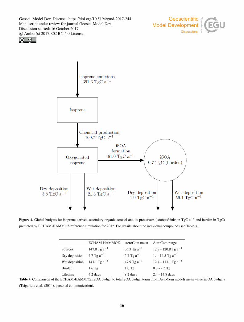
Figure 4. Global budgets for isoprene derived secondary organic aerosol and its precursors (sources/sinks in TgC a−1 and burden in TgC)

predicted by ECHAM-HAMMOZ reference simulation for 2012. For details about the individual compounds see Table 3.

ECHAM-HAMMOZ AeroCom mean AeroCom range

Sources 147.8 Tg a−1 36.3 Tg a−1 12.7 - 120.8 Tg a−1

Dry deposition 4.7 Tg a−1 5.7 Tg a−1 1.4 -14.5 Tg a−1

Wet deposition 143.1 Tg a−1 47.9 Tg a−1 12.4 - 113.1 Tg a−1

Burden 1.6 Tg 1.0 Tg 0.3 - 2.3 Tg

Lifetime 4.2 days 8.2 days 2.4 - 14.8 daysTable 4. Comparison of the ECHAM-HAMMOZ iSOA budget to total SOA budget terms from AeroCom models mean value in OA budgets

(Tsigaridis et al. (2014), personal communication).

16


As stated in Hodzic et al. (2016), global models are missing aerosol sinks like in particle fragmentation and particle photol-

ysis and should therefore overestimate SOA formation. On the contrary, global models tend to underestimate SOA formation.

The comparison of ECHAM-HAMMOZ iSOA is to total SOA of other models shows that the criticized underestimation is

more than resolved, since no SOA from aromatics or terpenes is considered in this study. Including semi-explicit chemistry

and explicit partitioning leads in ECHAM-HAMMOZ to a high isoprene SOA yield, which motivated motivated several sensi-5

tivity runs.

3.2 Sensitivity runs

3.2.1 Comparison to pseudo chemistry SOA

As explained in Section 2.1.2 ECHAM-HAM with SALSA has an own module to simulate SOA formation via the VBS

system using pseudo chemistry to form SOA precursors. To compare the semi-explicit chemistry and explicit compound-wise10

partitioning to the pseudo chemistry and VBS system, an ECHAM-HAM run (RefVBS) was performed just including isoprene

emissions to form just iSOA in both models. From these isoprene emissions ECHAM-HAM produces gas phase compounds

of the VBS classes 0, 1 and 10. Therefore, also semi volatile compounds are included, which lack in RefBase. Conversely,

ECHAM-HAM does not include IEPOX and glyoxal SOA, thus here these two compounds are not included in the comparison.

Total iSOA formed by partitioning including SVOC and IVOC from ECHAM-HAM RefVBS is compared to iSOA from LVOC15

in ECHAM-HAMMOZ reference run RefBase.

The formed precursors in the gas phase from RefVBS compared to the LVOC from RefBase are shown in Figure 5. From

the higher gas phase concentrations, it can be seen that the VBS system also includes semi volatile compounds. Again, the

emission pattern of MEGAN is clearly visible on both model runs, just very low concentrations in RefBase hide some isoprene

emitting areas.20

Nevertheless, the low gas phase concentrations in RefBase do not mean, that less iSOA precursors were formed, in contrary

as can be seen in Figure 5 iSOA from LVOC in RefBase is overall higher and horizontally transported further than iSOA in

RefVBS. Local maxima match between both models, the higher values in Southeastern US and in the Amazon are captured

by both models. However, in Southeastern US RefBase simulates values around 6 µg m−3 over a broader area than RefVBS

reaching 3.5 µg m−3 in two more local maxima. Similarly, over the Amazon and north of the Andes RefBase simulates up to25

9 µg m−3 while RefVBS reaches 3 µg m−3. Both simulations also agree on a local maximum in Central Africa and over North

Australia and Indonesia. Again, peak concentrations differ, here by a factor of around 2.

Even if RefVBS includes also SVOC in their iSOA formation, particle concentrations are higher in RefBase. This results

from different chemical precursor formation, via semi-explicit MOZ LVOC are formed in an amount large enough to make

significant contributions to SOA mass. LISOPOOHOOH formations is not taken into account in the ECHAM-HAM pseudo30

chemistry formulation and explain comparably low iSOA yields accounted for.

17


Figure 5. Seasonal mean values of gas phase precursors (upper plots) and iSOA (lower plots) for June, Juli and August 2012 at the surface

layer. The reference run RefBase with ECHAM-HAMMOZ is shown on the left side, on the right the ECHAM-HAM RefVBS. For RefBase

the precursors consist of the four isoprene derived LVOC described above, for RefVBS the sum of gas phase VBS classes 0, 1 and 10 is

shown.

18


Figure 6. Surface aerosol concentrations for LIEPOX derived iSOA with uniform pH value used in the reference run (left) and with variable

pH value calculated with AIM aerosol thermodynamics model (see Section 2.2) in the sensitivity run γpH for the time period of June, July

and August 2012.

3.2.2 IEPOX sensitivity to aerosol pH

As discussed in Section 2.1.1, several laboratory and field studies suggested a pH value influence on the reactive uptake of

IEPOX. ECHAM-HAMMOZ does not include ammonium and nitrate aerosol, therefore no aerosol pH value can be obtained

by the model system. As described in Section 2.2 a simulation with AIM aerosol thermodynamics model was performed to

obtain the global aerosol pH distribution consistent to ECHAM-HAMMOZ aerosols (Figure S1). Aerosol pH distribution by5

AIM is used as input in the sensitivity simulation γpH, while the reference simulation RefBase uses a uniform value for the

reactive uptake coefficient γ corresponding to a pH of around 2.5. The simulation γpH was designed to to explore the impact of

such a dependence. Therefore, based on reaction probability values given in Eddingsaas et al. (2010) and Gaston et al. (2014)

a simple function for γIEPOX was formulated and implemented in ECHAM-HAMMOZ:

γ(pH) =

10−2, pH< 2

0.1[H+] + 10−4, pH ∈ [2,5]

0, pH> 5

(2)10

where [H+] is the concentration of protons H+ in the aerosol given in mol l−1. The reaction probability varies linearly

between particles of pH values between 2 and 5. For acidic particles the upper limit of 10−2 is fixed. For particles which are

not acidic enough (pH greater 5) no reaction is assumed. The pH distribution (Figure S1) was then used as model input values.

The pH value of the surface aerosols was applied to each model layer, but largest effect can be observed where acidic aerosol

and LIEPOX are present.15

19


Figure 6 shows the resulting global surface distribution of γpH run for northern hemispheric summer compared to RefBase.

Enhancement of reactive uptake in γpH over land is clearly visible, especially over Southeastern US maximum values are more

than doubled. Further, more areas with 3 - 4 µg m−3 over Africa, the Middle East and Eurasia can be found, where RefBASE

has values lower than 1 µg m−3. In contrast, suppression of LIEPOX reactive uptake is observable over the Amazon.

Total LIEPOX aerosol produced during this time period increased by 58% in γpH compared to RefBase. In RefBase an5

aerosol pH around 2.5 was assumed for all aerosols, also those which might be less acidic like sea salt aerosol. Nevertheless,

compared to γpH less LIEPOX-SOA was formed. In γpH most areas are covered by less acidic aerosol but LIEPOX is

produced or transported there, where acidic aerosol can be found, this leads to the observed increase in iSOA formation.

As an alternative explanation for the to pH value dependence, Xu et al. (2015) hypothesize that IEPOX uptake enhancement

could be triggered by sulfate aerosol. Although sulfate aerosol is simulated no sensitivity study was performed here due to lack10

of process understanding and possible reactive uptake parametrizations.

3.2.3 Sensitivity to evaporation enthalpy

Tsigaridis and Kanakidou (2003) point out the sensitivity of SOA formation to the evaporation enthalpy ∆Hvap. Nevertheless,

due to the lack of knowledge of ∆Hvap of the various different organic compounds, usually a fixed value or rather low value is

used for all of them (Epstein et al., 2009). Depending on the study, different estimations for ∆Hvap were made, ranging between15

30 and 156 kJ mol−1 (Athanasopoulou et al., 2012). Farina et al. (2010) also use the Clausius-Clapeyron equation to calculate

saturation concentrations for a variety of organics using for all of them 30 kJ mol−1. To explore the impact of this assumption

and the impact of a lower evaporation enthalpy, the sensitivity run ∆H30 was designed to use ∆Hvap =30 kJ mol−1 but

keeping the same reference saturation vapor pressure (see Table 1).

As an example Figure 7 shows the curves given by equation (1) using ∆Hvap of the reference run and the sensitivity run.20

Equation (1) changes its curve form drastically when lowering ∆Hvap from values around 150 kJ mol−1 to 30 kJ mol−1. For

temperatures lower than the reference value of 298.15 K the saturation vapor pressure of ∆H30 p∗∆H30 is higher compared to

the reference p∗, but for temperatures higher 298.15 K the opposite is the case (see Figure 7).

As a result, the impact of variable ∆Hvap on iSOA formation varies with temperature, therefore, also with region and

height. The sensitivity simulation ∆H30 ran for June, July and August 2012 with changed Clausius-Clapeyron equation curves25

according to Figure 7. Even during this northern hemispheric summer, on a global perspective the atmosphere is on average

cooler than 298.15 K, especially at higher altitudes. Therefore, global total iSOA production in ∆H30 for the considered time

period is just 0.6 TgC lower compared to RefBase. This is a reduction of 4% of the total amount produced in RefBase in June,

July and August 2012. For surface temperatures higher than 298.15 K p∗∆H30 is orders of magnitude lower than the reference

p∗, but gas phase concentrations of iSOA precursors are high enough, that no significant impact on iSOA concentrations is30

seen. In agreement, surface concentration fields do not change much and are therefore not shown.

The assumption made by Farina et al. (2010) connected with the estimation of LVOC p∗0 in this study therefore does not lead

to significant changes in model results. Lowest sensitivity to ∆Hvap can be found in the lowest LVOC, LISOPOOHOOH. In

20


Figure 7. Curves given by Clausius Clapeyron equation 1 for C59OOH. The red curve is obtained by setting ∆Hvap = 30 kJ mol−1, the

black one describes the parameters used in the reference run (see Table 1).

ECHAM-HAMMOZ sensitivity to ∆Hvap increases with volatility of the compounds, therefore ∆Hvap should be crucial for

additional consideration of SVOC and IVOC, which will be added to the model in a future study.

3.3 Uncertainty estimation saturation vapor pressure

As described in Section 2.1.1 the group contribution method by Nannoolal et al. (2008) in combination with the boiling

point method by Nannoolal et al. (2004) were used to obtain the saturation vapor pressure of originated isoprene products5

as a function of temperature. Group contribution methods estimate the contribution of functional groups on saturation vapor

pressure. The Nannoolal et al. (2008) group contribution method is based on 68835 data points of 1663 components and just

needs two inputs, the molecular structure and the normal boiling point. Nannoolal et al. (2008) report a good performance

against measurements. Nevertheless, when its performance is compared to compounds outside the training set, results become

worse (Barley and McFiggans, 2010; OMeara et al., 2014). Barley and McFiggans (2010) underline that databases are typically10

biased towards mono-functional groups and therefore, group contribution methods trained with these data perform well at

volatile fluids, but not for low volatility compounds. OMeara et al. (2014) arrive at similar conclusions, they tested seven

saturation vapor pressure estimation methods and found that even if Nannoolal et al. (2008) method results in the lowest mean

bias error, the method shows poor accuracy for compounds with low volatility. This tendency holds also true for the other

21


Nannoolal et al. (2008) Donahue et al. (2011)

LNISOOH 1.2 (1.4) 1.3

LISOPOOHOOH -1.6 (-1.9) -0.7

LC578OOH 1.1 (1.1) 1.

C59OOH 0.8 1.Table 5. Comparison logarithmic saturation concentrations log10C

∗0 at 300 K for the LVOCs calculated via the group contribution method

used here (Nannoolal et al., 2008) and a simple group contribution method formulated by Donahue et al. (2011). In brackets the log10C∗0 for

the isomers are shown.

tested methods showing an increasing error with increasing number of hydrogen bonds. This systematic error results in a SOA

formation overestimation. Moreover, McFiggans et al. (2010) analyzed the dependence of SOA formation of the saturation

vapor pressure of each compounds and state that SOA mass is highly sensitive to this parameter. Up to 30% overestimation can

result from ignoring non-ideality of the organic mixture.

These studies already identified and emphasized several causes and consequences of the various group contribution methods.5

Thus, log10C∗0 values are compared to a simple group method based on oxygen, carbon and nitrate atoms in the molecule

described in Donahue et al. (2011) (Table 5).

As can be seen from Table 5, the log10C∗0 values do not differ much between the simple group contribution method of

Donahue et al. (2011) and the one by Nannoolal et al. (2008), except for the lowest volatility compound LISOPOOHOOH.

For LISOPOOHOOH, Nannoolal et al. (2008) predict a much lower volatility than Donahue et al. (2011). This difference10

agrees with the findings of the studies described above and indicates that LISOPOOHOOH-iSOA formation might be too high

in ECHAM-HAMMOZ. Also given are the log10C∗0 values for the different isomers. Due to computational resource limits,

no further sensitivity runs were done. Nevertheless, from the log10C∗0 values and the values in Table 1 it is clear, that for

LC578OOH there is no difference caused by isomeric structures in volatility, for LNSISOOH the other isomer is even slightly

more volatile and for LISOPOOHOOH the opposite holds true, its second isomer is slightly less volatile. Since LNISOOH15

is only formed in very low concentrations these deviations might not be visible in iSOA formation. Similarly an even lower

volatility LISOPOOHOOH should also not change the main findings of this study, since it already dominates iSOA formation.

3.3.1 Comparison with observations

In order to evaluate how much of total organic aerosol (OA), including primary and secondary organic aerosol, are related

to iSOA, iSOA concentrations and O:C ratios from ECHAM-HAMMOZ are compared to atmospheric Atmospheric Mass20

Spectrometry (AMS) measurements from different field campaigns given in Table 6. Measurements were selected from AMS

global database (Zhang et al., last accessed on 22.09.2017) according to the availability of elemental ratios. All campaigns

took place either in Europe or North America and include six different countries. In Helsinki, Finland winter and spring

measurements are available.

22


Location Observation time period Reference

Helsinki, Finland (60.2◦ N, 24.95◦ E) 08.01. - 14.03.2009 (W) Carbone et al. (2014)

09.04. - 08.05.2009 (S) Timonen et al. (2010)

Mace Head, Ireland (53.33◦ N, 9.99◦ W) 25.02. - 26.03.2009 Dall’Osto et al. (2009)

Po Valley, Italy (44.65◦ N, 11.62◦ E) 31.03. - 20.04.2008 Saarikoski et al. (2012)

Houston, USA (29.8◦ N, 95.4◦ W) 15.08. - 15.09.2000 Zhang et al. (2007)

Mexico City, Mexico (19.48◦ N, 99.15◦ W) 10.03. - 30.03.2006 Aiken et al. (2009, 2010)

Manaus, Brazil (2.58◦ S,60.2◦ W) 06.02. - 13.03.2008 Chen et al. (2009); Pöschl et al. (2010); Martin et al. (2010)Table 6. Overview ambient measurement locations, time periods and references. For Helsinki there are two time series, one during winter

(W) and the second during spring (S).

Figure 8. Box plots showing the variability of concentrations measured and corresponding instantaneous values from ECHAM-HAMMOZ.

Countries of measurement campaigns are given. First, European countries then American ones. The shortcuts refer to: FiW=Helsinki, Finland

(Winter), FiS=Helsinki, Finland (Spring), Ire=Mace Head, Ireland, Ita=Po Valley, Italy, USA=Houston Texas, USA, Mex=Mexico City,

Mexico, Bra=Manaus, Brazil. The model time resolution is three hours, whereas all values given from the observations are included meaning

that they have a higher time resolution.

23


Figure 9. Similar to Figure 8 showing corresponding O:C ratios of the subset Houston Texas, USA and Manaus, Brazil. The O:C ratios

shwon here are corrected by the factor 1.27 according to Canagaratna et al. (2015)

Figure 8 shows the quartiles of the time series of the concentrations in the different locations, from left to right first the four

European data sets and then the American ones. The European data sets display a variety of local OA sources. For Helsinki,

Carbone et al. (2014) report a variety of local sources for OA including biomass burning, traffic, coffee roaster and also SOA

from long range transport. In Mace Head two different OA types are measured depending on the advection of either marine

air or continental air (Dall’Osto et al., 2009). Saarikoski et al. (2012) identified in Po Valley a complex mixture of OA was5

with local and regional sources, mainly from anthropogenic origin. For Finland, Ireland and Italy, ECHAM-HAMMOZ reveals

a minor contribution of iSOA to OA this can be explained by the measurement time periods in winter or early spring where

vegetation in Europe does not emit large isoprene amounts (Steinbrecher et al., 2009).

Looking at the concentrations measured in Houston Texas, USA it can be seen that a great part of the variability is cap-

tured by iSOA, which is explained by high isoprene emissions found in Southeastern US. ECHAM-HAMMOZ median and10

percentiles are still lower than the observations since the observation includes total OA. The organic aerosol in Mexico City

was measured at an urban super-site and covers such a big range of concentrations, which are dominated by anthropogenic

emissions including biomass burning, nitrogen containing OA and primary hydrocarbon like OA associated with traffic (Aiken

24


et al., 2009). According to the concentrations simulated by ECHAM-HAMMOZ, just a minor part of these can be explained by

iSOA. Manaus, Brazil is located in the Amazon Basin and classified as pristine environment close to pre-industrial conditions

(Pöschl et al., 2010; Martin et al., 2010). Therefore, the particles are nearly pure biogenic and Martin et al. (2010) report an

upper limit of 5% primary organic aerosol. These conditions are ideal to compare them to ECHAM-HAMMOZ just including

iSOA, because isoprene emissions are high in the Amazon Basin and should dominate the OA there. As can be seen in Figure 8,5

HAMMOZ simulates overall higher iSOA concentrations that OA concentrations measured. Moreover, higher peak values are

simulated and the median is higher than the upper 1.5 inter-quartile range whisker of observed concentrations.

For Houston Texas and Manaus, ECHAM-HAMMOZ relates a great part of the OA to iSOA, to further investigate this, O:C

ratios are compared too. Due to restricted iSOA formation in ECHAM-HAMMOZ just from LVOC which are highly oxidized

molecules with molecular O:C ratios between 0.6 and 1.4, the modeled O:C ratio just covers small variability and is around 110

in both regions, see Figure 9.

The comparison of concentration spectrum in Houston Texas showed a great part to be attributed to iSOA, this modeled

subset covers upper values of the O:C ratio between 0.8 and 1.1, which still lie within the 75th percentile and the upper

1.5×IQR whisker of the measured data. This is related to the fact of missing SVOC and IVOC usually having lower O:C ratios

and the contribution of POA to OA, which is not included in this comparison, because no assumptions of POA O:C ratios are15

made.

In contrast, the OA measured in Manaus located at the Amazon Basin, which consists of 95% SOA does not show as high

O:C ratios as iSOA modeled by ECHAM-HAMMOZ. The median of observed aerosol lies at 0.4, instead of 1. Certainly part

of it is explained by missing SVOC and IVOC in ECHAM-HAMMOZ, but might also be related to SOA from other organic

molecules than isoprene. For Manaus an overestimation of iSOA concentrations by the model might be related to mistakes in20

emissions and in the chemical mechanism, missing sink processes and uncertainties in p∗. In term of O:C ratio of modeled

iSOA between 0.6 and 1.4, the simulated values are covered by the ambient values in Houston Texas, but not in Manaus. This

points to SVOC, IVOC and SOA from other sources than isoprene.

To summarize, isoprene emissions are not dominating OA in Europe, therefore the model shows iSOA having a small

contribution to concentrations there. In contrast, American OA is more impacted by iSOA, especially in USA and Brazil.25

4 Discussion

The comparison of RefBase to the AeroCom models, ECHAM-HAM and AMS measurements in the isoprene dominated area

Manaus in the Amazon basin revealed that semi-explicit treatment of atmospheric chemistry, at least for isoprene leads to

much larger SOA production rates and eliminates low biases found in most other global model studies. In fact, especially over

Brazil, SOA now has a tendency to be overestimated. This points to the possible importance of aerosol sink processes which30

have not been included in the current ECHAM-HAMMOZ version. Kroll et al. (2006) reported rapid chemical loss of SOA

via photolysis could be a possibility to further transform iSOA either to higher oxidized molecules in the particle phase such

as oligomers, or to fragment iSOA compounds leading to VOC and iSOA reduction. Hodzic et al. (2015) explored the global

25


impact of SOA photolysis and report about a 40 - 60% mass reduction after 10 days. SOA photolysis is closely related to

wet-phase, in-particle chemistry, which is not included in the ECHAM-HAMMOZ chemical mechanism.

Extrapolating iSOA production rate to the production rate of SOA in ECHAM-HAMMOZ including SVOC, IVOC not

only from isoprene, but also from terpenes and aromatics, we expect to find a portion of SOA which cannot be reduced by

including the missing sinks known. Various reasons for this part of the overestimation of iSOA in ECHAM-HAMMOZ could5

be identified analyzing the results of the RefBase run and the several sensitivity runs.

First, overestimation of iSOA from isoprene derived LVOC already starts with the group contribution method used to esti-

mate the saturation vapor pressure and evaporation enthalpy of these compounds. As discussed in OMeara et al. (2014) and

Barley and McFiggans (2010) the Nannoolal et al. (2008) method is problematic in the low volatility range, giving too low

saturation pressures, which leads to an overestimation in SOA formation. Also comparing the logarithm of the saturation con-10

centration at a reference temperature (log10C∗0 ) to the simple method of Donahue et al. (2011) reveals greatest differences in

the lowest volatile compound LISOPOOHOOH pointing to the direction that the lowest volatile compound has most uncertain

log10C∗0 . Since LISOPOOHOOH is high in ECHAM-HAMMOZ, it has great impact on iSOA. LISOPOOHOOH log10C

∗0

might be higher and this would reduce the erroneous part of iSOA concentrations due to Nannoolal et al. (2008) method.

A second aspect leading to a high production in iSOA is the semi-explicit chemistry itself. Different chemical pathways15

lead to formation of isoprene LVOCs, some requiring NO and NO3 for the initial steps followed OH, HO2 or RO2. Forma-

tion of LVOCs via the NOx-depended pathway hardly happens, as can be seen in the chemical budget terms. LNISOOH and

LC578OOH are formed in very low concentrations and C59OOH might just result from the HO2-dominated pathway. From

the chemical branching it can be clearly seen that in JAM3 the OH initiated pathway is preferred, even in regions were NO

mixing ratios are higher than 200 pptv (not shown). 90% of iSOA consist of products from this pathway, mostly IEPOX20

and LISOPOOHOOH. For LIEPOX this might lead to a large overestimation when acidic enhancement is considered.

Highly acidic aerosol is expected in regions where sulfate pollution is high and these regions usually coincide with high NOx,

which should suppress LIEPOX formation. In the atmosphere, both processes compensate each other, but in γpH no NOx-

suppression takes place, only acidic enhancement leading to high LIEPOX-SOA concentrations. Further, LISPOOHOOH

production might be high due to missing intramolecular H-shift of LISOPOOHO2 which would lead to products with a sat-25

uration vapor pressure which is around 2 orders of magnitude higher than the one of LISPOOHOOH (see Section 2.1.1,

DAmbro et al. (2017b)). Both processes as represented in ECHAM-HAMMOZ lead to an upper estimate of iSOA formation

by these to isoprene oxidation products.

Third, the main iSOA formation pathways follow from OH initiated reactions, which is the main oxidation pathway for

isoprene. Nevertheless, analysis from Schultz et al. (submitted) shows that due to problems in tropical dynamics of ECHAM6,30

the tropical region is too wet leading to a higher production of OH radicals and therefore is more oxidative than the real

atmosphere. Tropical regions are those, where most of isoprene is emitted. Thus, gas phase precursor formation might be

overestimated already, which translates into an iSOA overestimation. Moreover, there simply might be a lack of understanding

of SOA formation in tropical regions, Lin et al. (2012) also found an overestimation of their modeled SOA compared to

26


measurements of tropical forest sited and conclude that more measurements and model studies are needed to improve the

formation mechanism in the tropics.

Finally, model limitations in aerosol and cloud processing did not allow to implement in-cloud iSOA formation. This is

not only a potential additional source, but also an additional sink. ECHAM-HAMMOZ just includes wet scavenging based

on solubility following Henry’s law, but according to Cole-Filipiak et al. (2010) the IEPOX hydrolysis reactions at low pH5

values have life times comparable to wet deposition. Heterogeneous uptake of IEPOX in cloud droplets and rain would lead

to a decrease in gas phase concentrations without resulting in iSOA, because it is lost immediately due to precipitation. This

would lower iSOA from LIEPOX, which now has a substantial contribution to total iSOA.

5 Conclusions

For the first time, the semi-explicit chemical treatment of isoprene oxidation in the chemical mechanism of a global chemistry10

climate model was connected to explicit partitioning of individual low volatility species according to their chemical structures.

The chemistry model MOZ includes a total of 779 reactions, where 147 reactions describe the isoprene oxidation. Isoprene

oxidation in MOZ leads to LVOCs which are explicitly partitioned and followed in specific aerosol bins by HAM-SALSA.

The partitioning is based on the saturation vapor pressure derived from the molecular structure of each single compound.

Furthermore, also reactive uptake of isoprene derived glyoxal and IEPOX was considered.15

These two iSOA formation pathways lead to an isoprene SOA yield of 16% relative to the primary oxidation of isoprene

by OH, NO3, and ozone in 2012. It was identified that in ECHAM-HAMMOZ most iSOA is produced via the OH oxidation

initiated pathway which leads to production of IEPOX and ISOP(OOH)2, a compound recently detected in experimental

studies. Together modeled IEPOX and ISOP(OOH)2 yield a fraction of 86% of total iSOA mass. In total 61 TgC iSOA are

produced. IEPOX forms 24.4 TgC and ISOP(OOH)2 28.3 TgC. 59.1 TgC iSOA are lost due to wet deposition, which is the20

main sink for iSOA in ECHAM-HAMMOZ. For 2012 an average iSOA burden of 0.7 TgC is calculated. These values were

compared to SOA budgets in AeroCom models. ECHAM-HAMMOZ simulates a higher production rate than all models used

in this AeroCom study.

Moreover, this explicit model system enables process understanding and discussion. While exploring the influence of aerosol

pH on IEPOX reactive uptake, enhancement of iSOA formation was found especially over Southeastern US while suppression25

could be observed over the Amazon basin.

Evaporation enthalpy used in previous model studies was compared to the explicitly derived evaporation enthalpy used in

ECHAM-HAMMOZ. A huge difference could be found in Clausius-Clapeyron curves, which does not translate to a big impact

on iSOA formation due to the fact that only LVOC were used.

Comparison of ECHAM-HAMMOZ iSOA concentrations to AMS measurements showed that ECHAM-HAMMOZ does30

not underestimate iSOA formation. On the contrary, in isoprene dominated regions like Brazil an iSOA overestimation could

be observed which gives the possibility to explore novel SOA sinks, like in-particle decomposition or photolysis. Not lowering

the production rate, but including additional sinks is the strategy proposed by Hodzic et al. (2016). They conclude that because

27


several SOA sinks are currently excluded from global models, these models are expected to overestimate SOA concentrations.

Instead of the expected overestimation, an underestimation is found in the majority of global models. With our explicit model

system connecting the aerosol bin scheme SALSA with the chemistry model MOZ in the frame of the global model ECHAM-

HAMMOZ sufficient SOA is produced to be able to explore new sink processes.

Code availability. The ECHAM6.3-HAM2.3MOZ1.0 model code can be found at https://redmine.hammoz.ethz.ch/projects/hammoz/wiki/5

Echam630-ham23-moz10. After registration the code is available for download via the Apache Subversion system (SVN). All changes made

according to SALSA and MOZ coupling can also be found there in the Finnish Meteorological Institute (FMI) branch. Please do not hesitate

to ask the authors for support getting the code.

Competing interests. No competing interests are present.

Acknowledgements. ECHAM-HAMMOZ simulations were supported by the Forschungszentrum Jülich and performed at the Jülich Su-10

percomputing Centre (2016). We also want to thank Q. Zhang, C. Parworth, M. Lechner, and J.L. Jimenez for facilitating the comparison

with observations with their AMS global database. K. Tsigaridis is acknowledged for sending detailed results from the AeroCom model

inter-comparison. Further, we acknowledge the authors involved in measuring organic aerosol in the different campaigns shown in this study.

28


References

Aiken, A., Salcedo, D., Cubison, M. J., Huffman, J., DeCarlo, P., Ulbrich, I. M., Docherty, K. S., Sueper, D., Kimmel, J., Worsnop, D. R.,

et al.: Mexico City aerosol analysis during MILAGRO using high resolution aerosol mass spectrometry at the urban supersite (T0)–Part

1: Fine particle composition and organic source apportionment, Atmospheric Chemistry and Physics, 9, 6633–6653, 2009.

Aiken, A., Foy, B. d., Wiedinmyer, C., DeCarlo, P., Ulbrich, I. M., Wehrli, M., Szidat, S., Prevot, A., Noda, J., Wacker, L., et al.: Mexico city5

aerosol analysis during MILAGRO using high resolution aerosol mass spectrometry at the urban supersite (T0)–Part 2: Analysis of the

biomass burning contribution and the non-fossil carbon fraction, Atmospheric chemistry and physics, 10, 5315–5341, 2010.

Athanasopoulou, E., Vogel, H., Vogel, B., Tsimpidi, A., Pandis, S. N., Knote, C., and Fountoukis, C.: Modeling the meteorological and

chemical effects of secondary organic aerosols during an EUCAARI campaign, Atmospheric Chemistry and Physics, 13, 625, 2012.

Barley, M. and McFiggans, G.: The critical assessment of vapour pressure estimation methods for use in modelling the formation of atmo-10

spheric organic aerosol, Atmospheric Chemistry and Physics, 10, 749–767, 2010.

Bergman, T., Kerminen, V.-M., Korhonen, H., Lehtinen, K., Makkonen, R., Arola, A., Mielonen, T., Romakkaniemi, S., Kulmala, M., and

Kokkola, H.: Evaluation of the sectional aerosol microphysics module SALSA implementation in ECHAM5-HAM aerosol-climate model,

Geoscientific Model Development, 5, 845–868, 2012.

Berndt, T., Herrmann, H., Sipilä, M., and Kulmala, M.: Highly Oxidized Second-Generation Products from the Gas-Phase Reaction of OH15

Radicals with Isoprene, J. Phys. Chem. A, 120, 10 150–10 159, 2016.

Canagaratna, M., Jimenez, J., Kroll, J., Chen, Q., Kessler, S., Massoli, P., Hildebrandt Ruiz, L., Fortner, E., Williams, L., Wilson, K.,

et al.: Elemental ratio measurements of organic compounds using aerosol mass spectrometry: characterization, improved calibration, and

implications, Atmospheric Chemistry and Physics, 15, 253–272, 2015.

Carbone, S., Aurela, M., Saarnio, K., Saarikoski, S., Timonen, H., Frey, A., Sueper, D., Ulbrich, I. M., Jimenez, J. L., Kulmala, M., et al.:20

Wintertime aerosol chemistry in sub-Arctic urban air, Aerosol Science and Technology, 48, 313–323, 2014.

Chen, Q., Farmer, D., Schneider, J., Zorn, S., Heald, C., Karl, T., Guenther, A., Allan, J., Robinson, N., Coe, H., et al.: Mass spectral

characterization of submicron biogenic organic particles in the Amazon Basin, Geophysical Research Letters, 36, 2009.

Claeys, M., Graham, B., Vas, G., Wang, W., Vermeylen, R., Pashynska, V., Cafmeyer, J., Guyon, P., Andreae, M. O., Artaxo, P., et al.:

Formation of secondary organic aerosols through photooxidation of isoprene, Science, 303, 1173–1176, 2004.25

Clegg, S. L., Brimblecombe, P., and Wexler, A. S.: Thermodynamic Model of the System H+- NH4+- Na+- SO42– NO3– Cl– H2O at 298.15

K, The Journal of Physical Chemistry A, 102, 2155–2171, 1998.

Clements, A. L. and Seinfeld, J. H.: Detection and quantification of 2-methyltetrols in ambient aerosol in the southeastern United States,

Atmospheric Environment, 41, 1825–1830, 2007.

Cole-Filipiak, N. C., OConnor, A. E., and Elrod, M. J.: Kinetics of the hydrolysis of atmospherically relevant isoprene-derived hydroxy30

epoxides, Environmental science & technology, 44, 6718–6723, 2010.

Dall’Osto, M., Ceburnis, D., Martucci, G., Bialek, J., Dupuy, R., Jennings, S., Berresheim, H., Wenger, J., Sodeau, J., Healy, R., et al.:

Aerosol properties associated with air masses arriving into the North East Atlantic during the 2008 Mace Head EUCAARI intensive

observing period: an overview., Atmospheric Chemistry & Physics Discussions, 9, 2009.

DAmbro, E. L., Lee, B. H., Liu, J., Shilling, J. E., Gaston, C. J., Lopez-Hilfiker, F. D., Schobesberger, S., Zaveri, R. A., Mohr, C., Lutz,35

A., et al.: Molecular composition and volatility of isoprene photochemical oxidation secondary organic aerosol under low-and high-NO x

conditions, Atmospheric Chemistry and Physics, 17, 159–174, 2017a.

29


DAmbro, E. L., Møller, K. H., Lopez-Hilfiker, F. D., Schobesberger, S., Liu, J., Shilling, J. E., Lee, B. H., Kjaergaard, H. G., and Thornton,

J. A.: Isomerization of Second-Generation Isoprene Peroxy Radicals: Epoxide Formation and Implications for Secondary Organic Aerosol

Yields, Environmental Science & Technology, 51, 4978–4987, 2017b.

De Gouw, J. and Jimenez, J. L.: Organic aerosols in the Earths atmosphere, 2009.

Dentener, F., Kinne, S., Bond, T., Boucher, O., Cofala, J., Generoso, S., Ginoux, P., Gong, S., Hoelzemann, J., Ito, A., et al.: Emissions of5

primary aerosol and precursor gases in the years 2000 and 1750 prescribed data-sets for AeroCom, Atmospheric Chemistry and Physics,

6, 4321–4344, 2006.

Donahue, N., Robinson, A., Stanier, C., and Pandis, S.: Coupled partitioning, dilution, and chemical aging of semivolatile organics, Environ-

mental Science & Technology, 40, 2635–2643, 2006.

Donahue, N. M., Robinson, A. L., and Pandis, S. N.: Atmospheric organic particulate matter: From smoke to secondary organic aerosol,10

Atmospheric Environment, 43, 94–106, 2009.

Donahue, N. M., Epstein, S., Pandis, S. N., and Robinson, A. L.: A two-dimensional volatility basis set: 1. organic-aerosol mixing thermo-

dynamics, Atmospheric Chemistry and Physics, 11, 3303–3318, 2011.

Eddingsaas, N. C., VanderVelde, D. G., and Wennberg, P. O.: Kinetics and products of the acid-catalyzed ring-opening of atmospherically

relevant butyl epoxy alcohols, The Journal of Physical Chemistry A, 114, 8106–8113, 2010.15

Emmons, L., Walters, S., Hess, P., Lamarque, J.-F., Pfister, G., Fillmore, D., Granier, C., Guenther, A., Kinnison, D., Laepple, T., et al.:

Description and evaluation of the Model for Ozone and Related chemical Tracers, version 4 (MOZART-4), Geoscientific Model Develop-

ment, 3, 43–67, 2010.

Epstein, S. A., Riipinen, I., and Donahue, N. M.: A semiempirical correlation between enthalpy of vaporization and saturation concentration

for organic aerosol, Environmental science & technology, 44, 743–748, 2009.20

Ervens, B. and Volkamer, R.: Glyoxal processing by aerosol multiphase chemistry: towards a kinetic modeling framework of secondary

organic aerosol formation in aqueous particles, Atmospheric Chemistry and Physics, 10, 8219–8244, 2010.

Farina, S. C., Adams, P. J., and Pandis, S. N.: Modeling global secondary organic aerosol formation and processing with the volatility basis

set: Implications for anthropogenic secondary organic aerosol, Journal of Geophysical Research: Atmospheres, 115, 2010.

Fröhlich-Nowoisky, J., Kampf, C. J., Weber, B., Huffman, J. A., Pöhlker, C., Andreae, M. O., Lang-Yona, N., Burrows, S. M., Gunthe, S. S.,25

Elbert, W., et al.: Bioaerosols in the Earth system: Climate, health, and ecosystem interactions, Atmospheric Research, 182, 346–376,

2016.

Fu, T.-M., Jacob, D. J., Wittrock, F., Burrows, J. P., Vrekoussis, M., and Henze, D. K.: Global budgets of atmospheric glyoxal and methyl-

glyoxal, and implications for formation of secondary organic aerosols, Journal of geophysical research: atmospheres, 113, 2008.

Fuzzi, S., Baltensperger, U., Carslaw, K., Decesari, S., Denier Van Der Gon, H., Facchini, M., Fowler, D., Koren, I., Langford, B., Lohmann,30

U., et al.: Particulate matter, air quality and climate: lessons learned and future needs, Atmospheric chemistry and physics, 15, 8217–8299,

2015.

Gaston, C. J., Riedel, T. P., Zhang, Z., Gold, A., Surratt, J. D., and Thornton, J. A.: Reactive uptake of an isoprene-derived epoxydiol to

submicron aerosol particles, Environmental science & technology, 48, 11 178–11 186, 2014.

Ghan, S. J. and Schwartz, S. E.: Aerosol properties and processes: A path from field and laboratory measurements to global climate models,35

Bulletin of the American Meteorological Society, 88, 1059–1083, 2007.

Goldstein, A. H. and Galbally, I. E.: Known and unexplored organic constituents in the earth’s atmosphere, 2007.

30


Guenther, A., Karl, T., Harley, P., Wiedinmyer, C., Palmer, P., and Geron, C.: Estimates of global terrestrial isoprene emissions using MEGAN

(Model of Emissions of Gases and Aerosols from Nature), Atmospheric Chemistry and Physics Discussions, 6, 107–173, 2006.

Hallquist, M., Wenger, J., Baltensperger, U., Rudich, Y., Simpson, D., Claeys, M., Dommen, J., Donahue, N., George, C., Goldstein, A., et al.:

The formation, properties and impact of secondary organic aerosol: current and emerging issues, Atmospheric Chemistry and Physics, 9,

5155–5236, 2009.5

Heald, C. L., Jacob, D. J., Park, R. J., Russell, L. M., Huebert, B. J., Seinfeld, J. H., Liao, H., and Weber, R. J.: A large organic aerosol source

in the free troposphere missing from current models, Geophysical Research Letters, 32, 2005.

Henrot, A.-J., Stanelle, T., Schröder, S., Siegenthaler, C., Taraborrelli, D., and Schultz, M. G.: Implementation of the MEGAN (v2. 1)

biogenic emission model in the ECHAM6-HAMMOZ chemistry climate model, Geoscientific Model Development, 10, 903, 2017.

Hodzic, A., Madronich, S., Kasibhatla, P., Tyndall, G., Aumont, B., Jimenez, J., Lee-Taylor, J., and Orlando, J.: Organic photolysis reactions10

in tropospheric aerosols: effect on secondary organic aerosol formation and lifetime, Atmospheric Chemistry and Physics, 15, 9253–9269,

2015.

Hodzic, A., Kasibhatla, P. S., Jo, D. S., Cappa, C. D., Jimenez, J. L., Madronich, S., and Park, R. J.: Rethinking the global secondary organic

aerosol (SOA) budget: stronger production, faster removal, shorter lifetime, Atmospheric Chemistry and Physics, 16, 7917–7941, 2016.

IPCC: Annex I: Atlas of Global and Regional Climate Projections, book section AI, pp. 1311–1394, Cambridge University Press, Cambridge,15

United Kingdom and New York, NY, USA, https://doi.org/10.1017/CBO9781107415324.029, www.climatechange2013.org, 2013.

Jimenez, J., Canagaratna, M., Donahue, N., Prevot, A., Zhang, Q., Kroll, J. H., DeCarlo, P. F., Allan, J. D., Coe, H., Ng, N., et al.: Evolution

of organic aerosols in the atmosphere, Science, 326, 1525–1529, 2009.

Jülich Supercomputing Centre: JURECA: General-purpose supercomputer at Jülich Supercomputing Centre, Journal of large-scale research

facilities, 2, https://doi.org/10.17815/jlsrf-2-121, http://dx.doi.org/10.17815/jlsrf-2-121, 2016.20

Kanakidou, M., Seinfeld, J., Pandis, S., Barnes, I., Dentener, F., Facchini, M., Dingenen, R. V., Ervens, B., Nenes, A., Nielsen, C., et al.:

Organic aerosol and global climate modelling: a review, Atmospheric Chemistry and Physics, 5, 1053–1123, 2005.

Kavouras, I. G., Mihalopoulos, N., and Stephanou, E. G.: Secondary organic aerosol formation vs primary organic aerosol emission: In

situ evidence for the chemical coupling between monoterpene acidic photooxidation products and new particle formation over forests,

Environmental science & technology, 33, 1028–1037, 1999.25

Kinnison, D., Brasseur, G., Walters, S., Garcia, R., Marsh, D., Sassi, F., Harvey, V., Randall, C., Emmons, L., Lamarque, J., et al.: Sensi-

tivity of chemical tracers to meteorological parameters in the MOZART-3 chemical transport model, Journal of Geophysical Research:

Atmospheres (1984–2012), 112, 2007.

Kokkola, H., Korhonen, H., Lehtinen, K., Makkonen, R., Asmi, A., Järvenoja, S., Anttila, T., Partanen, A.-I., Kulmala, M., Järvinen, H.,

et al.: SALSA–a Sectional Aerosol module for Large Scale Applications, Atmospheric Chemistry and Physics, 8, 2469–2483, 2008.30

Kourtchev, I., Ruuskanen, T., Maenhaut, W., Kulmala, M., and Claeys, M.: Observation of 2-methyltetrols and related photo-oxidation

products of isoprene in boreal forest aerosols from Hyytiälä, Finland, Atmospheric Chemistry and Physics, 5, 2761–2770, 2005.

Kroll, J. H., Ng, N. L., Murphy, S. M., Flagan, R. C., and Seinfeld, J. H.: Secondary organic aerosol formation from isoprene photooxidation,

Environmental science & technology, 40, 1869–1877, 2006.

Kühn, T., Merikanto, J., Mielonen, T., Stadtler, S., Hienola, A., Korhonen, H., Ferrachat, S., Lohmann, U., Neubauer, D., Tegen, I.,35

Siegenthaler-Le Drian, C., Wahl, S., Schultz, M. G., Rast, S., Schmidt, H., Stier, P., Lehtinen, K., and Kokkola, H.: SALSA2.0 part2:

Implementation of a volatility basis set to model formation of secondary organic aerosol, in preparation.

31


Lakey, P. S., Berkemeier, T., Tong, H., Arangio, A. M., Lucas, K., Pöschl, U., and Shiraiwa, M.: Chemical exposure-response relationship

between air pollutants and reactive oxygen species in the human respiratory tract, Scientific reports, 6, 32 916, 2016.

Lal, V., Khalizov, A. F., Lin, Y., Galvan, M. D., Connell, B. T., and Zhang, R.: Heterogeneous reactions of epoxides in acidic media, The

Journal of Physical Chemistry A, 116, 6078–6090, 2012.

Lamarque, J.-F., Bond, T. C., Eyring, V., Granier, C., Heil, A., Klimont, Z., Lee, D., Liousse, C., Mieville, A., Owen, B., et al.: Histor-5

ical (1850–2000) gridded anthropogenic and biomass burning emissions of reactive gases and aerosols: methodology and application,

Atmospheric Chemistry and Physics, 10, 7017–7039, 2010.

Lelieveld, J., Gromov, S., Pozzer, A., and Taraborrelli, D.: Global tropospheric hydroxyl distribution, budget and reactivity, Atmos. Chem.

Phys, 16, 12 477–12 493, 2016.

Li, N., Fu, T.-M., Cao, J., Lee, S., Huang, X.-F., He, L.-Y., Ho, K.-F., Fu, J. S., and Lam, Y.-F.: Sources of secondary organic aerosols in the10

Pearl River Delta region in fall: Contributions from the aqueous reactive uptake of dicarbonyls, Atmospheric environment, 76, 200–207,

2013.

Liggio, J., Li, S.-M., and McLaren, R.: Heterogeneous reactions of glyoxal on particulate matter: Identification of acetals and sulfate esters,

Environmental science & technology, 39, 1532–1541, 2005a.

Liggio, J., Li, S.-M., and McLaren, R.: Reactive uptake of glyoxal by particulate matter, Journal of Geophysical Research: Atmospheres,15

110, 2005b.

Lin, G., Penner, J., Sillman, S., Taraborrelli, D., and Lelieveld, J.: Global modeling of SOA formation from dicarbonyls, epoxides, organic

nitrates and peroxides, Atmospheric Chemistry and Physics, 12, 4743–4774, 2012.

Lin, S.-J. and Rood, R. B.: Multidimensional flux-form semi-Lagrangian transport schemes, Monthly Weather Review, 124, 2046–2070,

1996.20

Lin, Y.-H., Knipping, E., Edgerton, E., Shaw, S., and Surratt, J.: Investigating the influences of SO2 and NH3 levels on isoprene-derived

secondary organic aerosol formation using conditional sampling approaches, Atmospheric Chemistry and Physics, 13, 8457–8470, 2013a.

Lin, Y.-H., Zhang, H., Pye, H. O., Zhang, Z., Marth, W. J., Park, S., Arashiro, M., Cui, T., Budisulistiorini, S. H., Sexton, K. G., et al.: Epoxide

as a precursor to secondary organic aerosol formation from isoprene photooxidation in the presence of nitrogen oxides, Proceedings of

the National Academy of Sciences, 110, 6718–6723, 2013b.25

Liu, J., DAmbro, E. L., Lee, B. H., Lopez-Hilfiker, F. D., Zaveri, R. A., Rivera-Rios, J. C., Keutsch, F. N., Iyer, S., Kurten, T., Zhang, Z., et al.:

Efficient isoprene secondary organic aerosol formation from a non-IEPOX pathway, Environmental science & technology, 50, 9872–9880,

2016.

Lopez-Hilfiker, F., Mohr, C., DAmbro, E. L., Lutz, A., Riedel, T. P., Gaston, C. J., Iyer, S., Zhang, Z., Gold, A., Surratt, J. D., et al.:

Molecular composition and volatility of organic aerosol in the Southeastern US: implications for IEPOX derived SOA, Environmental30

science & technology, 50, 2200–2209, 2016.

Marais, E. A., Jacob, D. J., Jimenez, J. L., Campuzano-Jost, P., Day, D. A., Hu, W., Krechmer, J., Zhu, L., Kim, P. S., Miller, C. C., et al.:

Aqueous-phase mechanism for secondary organic aerosol formation from isoprene: application to the southeast United States and co-

benefit of SO 2 emission controls, Atmospheric Chemistry and Physics, 16, 1603–1618, 2016.

Martin, S., Andreae, M., Althausen, D., Artaxo, P., Baars, H., Borrmann, S., Chen, Q., Farmer, D., Guenther, A., Gunthe, S., et al.: An35

overview of the Amazonian aerosol characterization experiment 2008 (AMAZE-08), Atmospheric Chemistry and Physics, 10, 2010.

32


McFiggans, G., Topping, D., and Barley, M.: The sensitivity of secondary organic aerosol component partitioning to the predictions of

component properties–Part 1: A systematic evaluation of some available estimation techniques, Atmospheric Chemistry and Physics, 10,

10 255–10 272, 2010.

McNeill, V. F., Woo, J. L., Kim, D. D., Schwier, A. N., Wannell, N. J., Sumner, A. J., and Barakat, J. M.: Aqueous-phase secondary organic

aerosol and organosulfate formation in atmospheric aerosols: a modeling study, Environmental science & technology, 46, 8075–8081,5

2012.

Nannoolal, Y., Rarey, J., Ramjugernath, D., and Cordes, W.: Estimation of pure component properties: Part 1. Estimation of the normal

boiling point of non-electrolyte organic compounds via group contributions and group interactions, Fluid Phase Equilibria, 226, 45–63,

2004.

Nannoolal, Y., Rarey, J., and Ramjugernath, D.: Estimation of pure component properties: Part 3. Estimation of the vapor pressure of non-10

electrolyte organic compounds via group contributions and group interactions, Fluid Phase Equilibria, 269, 117–133, 2008.

Nölscher, A., Butler, T., Auld, J., Veres, P., Muñoz, A., Taraborrelli, D., Vereecken, L., Lelieveld, J., and Williams, J.: Using total OH

reactivity to assess isoprene photooxidation via measurement and model, Atmospheric Environment, 89, 453–463, 2014.

Nozière, B., González, N. J., Borg-Karlson, A.-K., Pei, Y., Redeby, J. P., Krejci, R., Dommen, J., Prevot, A. S., and Anthonsen, T.: Atmo-

spheric chemistry in stereo: A new look at secondary organic aerosols from isoprene, Geophysical Research Letters, 38, 2011.15

ODonnell, D., Tsigaridis, K., and Feichter, J.: Estimating the direct and indirect effects of secondary organic aerosols using ECHAM5-HAM,

Atmospheric Chemistry and Physics, 11, 8635–8659, 2011.

Odum, J. R., Hoffmann, T., Bowman, F., Collins, D., Flagan, R. C., and Seinfeld, J. H.: Gas/particle partitioning and secondary organic

aerosol yields, Environmental Science & Technology, 30, 2580–2585, 1996.

OMeara, S., Booth, A. M., Barley, M. H., Topping, D., and McFiggans, G.: An assessment of vapour pressure estimation methods, Physical20

Chemistry Chemical Physics, 16, 19 453–19 469, 2014.

Pandis, S. N., Harley, R. A., Cass, G. R., and Seinfeld, J. H.: Secondary organic aerosol formation and transport, Atmospheric Environment.

Part A. General Topics, 26, 2269–2282, 1992.

Pankow, J. F.: An absorption model of gas/particle partitioning of organic compounds in the atmosphere, Atmospheric Environment, 28,

185–188, 1994.25

Paulot, F., Crounse, J. D., Kjaergaard, H. G., Kürten, A., Clair, J. M. S., Seinfeld, J. H., and Wennberg, P. O.: Unexpected epoxide formation

in the gas-phase photooxidation of isoprene, Science, 325, 730–733, 2009.

Pöschl, U., Martin, S., Sinha, B., Chen, Q., Gunthe, S., Huffman, J., Borrmann, S., Farmer, D., Garland, R., Helas, G., et al.: Rainforest

aerosols as biogenic nuclei of clouds and precipitation in the Amazon, science, 329, 1513–1516, 2010.

Pye, H. O., Pinder, R. W., Piletic, I. R., Xie, Y., Capps, S. L., Lin, Y.-H., Surratt, J. D., Zhang, Z., Gold, A., Luecken, D. J., et al.: Epoxide30

pathways improve model predictions of isoprene markers and reveal key role of acidity in aerosol formation, Environmental science &

technology, 47, 11 056–11 064, 2013.

Riedel, T. P., Lin, Y.-H., Budisulistiorini, S. H., Gaston, C. J., Thornton, J. A., Zhang, Z., Vizuete, W., Gold, A., and Surratt, J. D.: Heteroge-

neous reactions of isoprene-derived epoxides: reaction probabilities and molar secondary organic aerosol yield estimates, Environmental

Science & Technology Letters, 2, 38–42, 2015.35

Riva, M., Budisulistiorini, S. H., Chen, Y., Zhang, Z., DAmbro, E. L., Zhang, X., Gold, A., Turpin, B. J., Thornton, J. A., Canagaratna, M. R.,

et al.: Chemical characterization of secondary organic aerosol from oxidation of isoprene hydroxyhydroperoxides, Environmental science

& technology, 50, 9889–9899, 2016.

33


Saarikoski, S., Carbone, S., Decesari, S., Giulianelli, L., Angelini, F., Canagaratna, M., Ng, N., Trimborn, A., Facchini, M., Fuzzi, S., et al.:

Chemical characterization of springtime submicrometer aerosol in Po Valley, Italy, Atmospheric Chemistry and Physics, 12, 8401–8421,

2012.

Schultz, M. G., Stadtler, S., Schroeder, S., Taraborrelli, D., Henrot, A., Kaffashzadeh, N., Franco, B., Ferrachat, S., Siegenthaler-Le Drian,

C., Lohmann, U., Neubauer, D., Wahl, S., Kokkola, H., Kuehn, T., Stier, P., Kinnison, D., Tyndall, G., and Orlando, J.: The Chemistry5

Climate Model ECHAM-HAMMOZ, Golbal Model Developement, submitted.

Schwartz, S. E.: Mass-transport considerations pertinent to aqueous phase reactions of gases in liquid-water clouds, in: Chemistry of multi-

phase atmospheric systems, pp. 415–471, Springer, 1986.

Seinfeld, J. H. and Pankow, J. F.: Organic atmospheric particulate material, Annual review of physical chemistry, 54, 121–140, 2003.

Shiraiwa, M., Li, Y., Tsimpidi, A. P., Karydis, V. A., Berkemeier, T., Pandis, S. N., Lelieveld, J., Koop, T., and Pöschl, U.: Global distribution10

of particle phase state in atmospheric secondary organic aerosols, Nature communications, 8, 2017.

Stadtler, S., Simpson, D., Schröder, S., Taraborrelli, D., Bott, A., and Schultz, M.: Ozone Impacts of Gas-Aerosol Uptake in Global Chemistry

Transport Models, Atmos. Chem. Phys., 2017.

Stein, O., Flemming, J., Inness, A., Kaiser, J. W., and Schultz, M. G.: Global reactive gases forecasts and reanalysis in the MACC project,

Journal of Integrative Environmental Sciences, 9, 57–70, 2012.15

Steinbrecher, R., Smiatek, G., Köble, R., Seufert, G., Theloke, J., Hauff, K., Ciccioli, P., Vautard, R., and Curci, G.: Intra-and inter-annual

variability of VOC emissions from natural and semi-natural vegetation in Europe and neighbouring countries, Atmospheric Environment,

43, 1380–1391, 2009.

Stevens, B., Giorgetta, M., Esch, M., Mauritsen, T., Crueger, T., Rast, S., Salzmann, M., Schmidt, H., Bader, J., Block, K., et al.: Atmospheric

component of the MPI-M Earth System Model: ECHAM6, Journal of Advances in Modeling Earth Systems, 5, 146–172, 2013.20

Stier, P., Feichter, J., Kinne, S., Kloster, S., Vignati, E., Wilson, J., Ganzeveld, L., Tegen, I., Werner, M., Balkanski, Y., et al.: The aerosol-

climate model ECHAM5-HAM, Atmospheric Chemistry and Physics, 5, 1125–1156, 2005.

Surratt, J. D., Murphy, S. M., Kroll, J. H., Ng, N. L., Hildebrandt, L., Sorooshian, A., Szmigielski, R., Vermeylen, R., Maenhaut, W., Claeys,

M., et al.: Chemical composition of secondary organic aerosol formed from the photooxidation of isoprene, The Journal of Physical

Chemistry A, 110, 9665–9690, 2006.25

Surratt, J. D., Kroll, J. H., Kleindienst, T. E., Edney, E. O., Claeys, M., Sorooshian, A., Ng, N. L., Offenberg, J. H., Lewandowski, M., Jaoui,

M., et al.: Evidence for organosulfates in secondary organic aerosol, Environmental Science & Technology, 41, 517–527, 2007a.

Surratt, J. D., Lewandowski, M., Offenberg, J. H., Jaoui, M., Kleindienst, T. E., Edney, E. O., and Seinfeld, J. H.: Effect of acidity on

secondary organic aerosol formation from isoprene, Environmental Science & Technology, 41, 5363–5369, 2007b.

Surratt, J. D., Chan, A. W., Eddingsaas, N. C., Chan, M., Loza, C. L., Kwan, A. J., Hersey, S. P., Flagan, R. C., Wennberg, P. O., and Seinfeld,30

J. H.: Reactive intermediates revealed in secondary organic aerosol formation from isoprene, Proceedings of the National Academy of

Sciences, 107, 6640–6645, 2010.

Taraborrelli, D., Lawrence, M., Butler, T., Sander, R., and Lelieveld, J.: Mainz Isoprene Mechanism 2 (MIM2): an isoprene oxidation

mechanism for regional and global atmospheric modelling, Atmospheric Chemistry and Physics, 9, 2751–2777, 2009.

Taraborrelli, D., Lawrence, M., Crowley, J., Dillon, T., Gromov, S., Groß, C., Vereecken, L., and Lelieveld, J.: Hydroxyl radical buffered by35

isoprene oxidation over tropical forests, Nature Geoscience, 5, 190, 2012.

34


Timonen, H., Aurela, M., Carbone, S., Saarnio, K., Saarikoski, S., Mäkelä, T., Kulmala, M., Kerminen, V.-M., Worsnop, D., and Hillamo,

R.: High time-resolution chemical characterization of the water-soluble fraction of ambient aerosols with PILS-TOC-IC and AMS, Atmo-

spheric Measurement Techniques, 3, 1063–1074, 2010.

Topping, D., Barley, M., Bane, M., Higham, N. J., Aumont, B., Dingle, N., and McFiggans, G.: UManSysProp v1. 0: an online

and open-source facility for molecular property prediction and atmospheric aerosol calculations, Geosci. Model. Dev., 9, 899–914,5

https://doi.org/https://doi.org/10.5194/gmd-9-899-2016, 2016.

Tsigaridis, K. and Kanakidou, M.: Global modelling of secondary organic aerosol in the troposphere: a sensitivity analysis, Atmospheric

Chemistry and Physics, 3, 1849–1869, 2003.

Tsigaridis, K., Daskalakis, N., Kanakidou, M., Adams, P., Artaxo, P., Bahadur, R., Balkanski, Y., Bauer, S., Bellouin, N., Benedetti, A., et al.:

The AeroCom evaluation and intercomparison of organic aerosol in global models, Atmospheric Chemistry and Physics, 14, 10 845–10

10 895, 2014.

Volkamer, R., Jimenez, J. L., San Martini, F., Dzepina, K., Zhang, Q., Salcedo, D., Molina, L. T., Worsnop, D. R., and Molina, M. J.:

Secondary organic aerosol formation from anthropogenic air pollution: Rapid and higher than expected, Geophysical Research Letters,

33, 2006.

Volkamer, R., San Martini, F., Molina, L. T., Salcedo, D., Jimenez, J. L., and Molina, M. J.: A missing sink for gas-phase glyoxal in Mexico15

City: Formation of secondary organic aerosol, Geophysical Research Letters, 34, 2007.

Washenfelder, R., Young, C., Brown, S., Angevine, W., Atlas, E., Blake, D., Bon, D., Cubison, M., De Gouw, J., Dusanter, S., et al.: The

glyoxal budget and its contribution to organic aerosol for Los Angeles, California, during CalNex 2010, Journal of Geophysical Research:

Atmospheres, 116, 2011.

Waxman, E. M., Dzepina, K., Ervens, B., Lee-Taylor, J., Aumont, B., Jimenez, J. L., Madronich, S., and Volkamer, R.: Secondary organic20

aerosol formation from semi-and intermediate-volatility organic compounds and glyoxal: Relevance of O/C as a tracer for aqueous multi-

phase chemistry, Geophysical Research Letters, 40, 978–982, 2013.

Woo, J. and McNeill, V.: simpleGAMMA v1. 0–a reduced model of secondary organic aerosol formation in the aqueous aerosol phase

(aaSOA), Geoscientific Model Development, 8, 1821–1829, 2015.

Xu, L., Guo, H., Boyd, C. M., Klein, M., Bougiatioti, A., Cerully, K. M., Hite, J. R., Isaacman-VanWertz, G., Kreisberg, N. M., Knote,25

C., et al.: Effects of anthropogenic emissions on aerosol formation from isoprene and monoterpenes in the southeastern United States,

Proceedings of the National Academy of Sciences, 112, 37–42, 2015.

Zhang, Q., Jimenez, J., Canagaratna, M., Allan, J., Coe, H., Ulbrich, I., Alfarra, M., Takami, A., Middlebrook, A., Sun, Y., et al.: Ubiquity

and dominance of oxygenated species in organic aerosols in anthropogenically-influenced Northern Hemisphere midlatitudes, Geophysical

Research Letters, 34, 2007.30

Zhang, Q., Parworth, C., Lechner, M., and Jimenez, J.: Aerosol Mass Spectrometer Global Database,

https://doi.org/doi:10.6084/m9.figshare.3486719, https://sites.google.com/site/amsglobaldatabase, last accessed on 22.09.2017.

35


Documents

Isoprene derived secondary organic aerosol in a global ...€¦ · Isoprene derived secondary organic aerosol in a global aerosol chemistry climate model ... which was further studied