econstorMake Your Publications Visible.

A Service of

zbwLeibniz-InformationszentrumWirtschaftLeibniz Information Centrefor Economics

Schrøter Joensen, Juanna; Skyt Nielsen, Helena

Working Paper

Is there a causal effect of high school math on labormarket outcomes?

IZA Discussion Papers, No. 2357

Provided in Cooperation with:IZA – Institute of Labor Economics

Suggested Citation: Schrøter Joensen, Juanna; Skyt Nielsen, Helena (2006) : Is there a causaleffect of high school math on labor market outcomes?, IZA Discussion Papers, No. 2357,Institute for the Study of Labor (IZA), Bonn,http://nbn-resolving.de/urn:nbn:de:101:1-20090622313

This Version is available at:http://hdl.handle.net/10419/34081

Standard-Nutzungsbedingungen:

Die Dokumente auf EconStor dürfen zu eigenen wissenschaftlichenZwecken und zum Privatgebrauch gespeichert und kopiert werden.

Sie dürfen die Dokumente nicht für öffentliche oder kommerzielleZwecke vervielfältigen, öffentlich ausstellen, öffentlich zugänglichmachen, vertreiben oder anderweitig nutzen.

Sofern die Verfasser die Dokumente unter Open-Content-Lizenzen(insbesondere CC-Lizenzen) zur Verfügung gestellt haben sollten,gelten abweichend von diesen Nutzungsbedingungen die in der dortgenannten Lizenz gewährten Nutzungsrechte.

Terms of use:

Documents in EconStor may be saved and copied for yourpersonal and scholarly purposes.

You are not to copy documents for public or commercialpurposes, to exhibit the documents publicly, to make thempublicly available on the internet, or to distribute or otherwiseuse the documents in public.

If the documents have been made available under an OpenContent Licence (especially Creative Commons Licences), youmay exercise further usage rights as specified in the indicatedlicence.

www.econstor.eu

IZA DP No. 2357

Is there a Causal Effect of High School Mathon Labor Market Outcomes?

Juanna Schrøter JoensenHelena Skyt Nielsen

DI

SC

US

SI

ON

PA

PE

R S

ER

IE

S

Forschungsinstitutzur Zukunft der ArbeitInstitute for the Studyof Labor

October 2006

Is there a Causal Effect of High School

Math on Labor Market Outcomes?

Juanna Schrøter Joensen University of Aarhus

Helena Skyt Nielsen

University of Aarhus and IZA Bonn

Discussion Paper No. 2357 October 2006

IZA

P.O. Box 7240 53072 Bonn

Germany

Phone: +49-228-3894-0 Fax: +49-228-3894-180

E-mail: iza@iza.org

Any opinions expressed here are those of the author(s) and not those of the institute. Research disseminated by IZA may include views on policy, but the institute itself takes no institutional policy positions. The Institute for the Study of Labor (IZA) in Bonn is a local and virtual international research center and a place of communication between science, politics and business. IZA is an independent nonprofit company supported by Deutsche Post World Net. The center is associated with the University of Bonn and offers a stimulating research environment through its research networks, research support, and visitors and doctoral programs. IZA engages in (i) original and internationally competitive research in all fields of labor economics, (ii) development of policy concepts, and (iii) dissemination of research results and concepts to the interested public. IZA Discussion Papers often represent preliminary work and are circulated to encourage discussion. Citation of such a paper should account for its provisional character. A revised version may be available directly from the author.

IZA Discussion Paper No. 2357 October 2006

ABSTRACT

Is there a Causal Effect of High School Math on Labor Market Outcomes?*

Outsourcing of jobs to low-wage countries has increased the focus on the accumulation of skills – such as Math skills – in high-wage countries. In this paper, we exploit a high school pilot scheme to identify the causal effect of advanced high school Math on labor market outcomes. The pilot scheme reduced the costs of choosing advanced Math because it allowed for at more flexible combination of Math with other courses. We find clear evidence of a causal relationship between Math and earnings for the students who are induced to choose Math after being exposed to the pilot scheme. The effect partly stems from the fact that these students end up with higher education. JEL Classification: I20, J24 Keywords: Math, high school curriculum, instrumental variable, local average treatment

effect Corresponding author: Helena Skyt Nielsen Department of Economics University of Aarhus Bartholins Allé 4, Bld. 322 DK-8000 Aarhus C Denmark E-mail: HNielsen@econ.au.dk

* Financial support from the Danish Research Agency is gratefully acknowledged. We appreciate useful comments from Joshua Angrist, Sandra Black, Nabanita Datta Gupta, Marianne Simonsen, Lars Skipper, Michael Svarer, Christopher Taber, as well as from discussants and participants at the DGPE, CEPR/IFAU/Uppsala University, CEPR/EENEE/University of Padova, and “Do Schools Matter?” Aarhus School of Business workshops, the SMYE 2006 and ESPE 2006 conferences, and we would like to thank seminar participants at U of Texas, U of Aarhus, Umeå University for comments on earlier drafts. The usual disclaimer applies.

1 Introduction

Increased global competition and outsourcing of jobs to low wage countrieshave placed increased focus on the e¢ ciency of the education system and theaccumulation of skills. As a result, there is much public discussion about theoptimal curriculum in many countries around the world. We devote this paperto study the e¤ect of Math, which is one of the core elements of all curricula inprimary and secondary schools.It is well established that individuals with advanced Math quali�cations

perform better on a range of important economic performance measures. Highschool graduates with advanced Math quali�cations have higher test scores, theyattain a higher education and they earn a higher income than others.1 Thequestion is, however, to what extent these observations indicate a causal impactof Math on performance, and to what extent it is a selection e¤ect indicatingthat people with other favorable characteristics choose to acquire higher Mathquali�cations.This question is closely related to the discussion of the human capital theory

of education versus the signaling theory of education. According to the humancapital theory, the Math premium indicates that more valuable skills are ac-quired during Math courses than during other coursework. Skills like clarity inexpressions, logical reasoning and inference are acquired and added to the stockof human capital and subsequently make the advanced Math students more pro-ductive. On the other hand, drawing on the signaling theory, advanced Mathworks as a signal which is cheaper to acquire for individuals with favorableskills, such as higher aptitude or motivation. Accordingly, it implies that theseemingly high return to advanced Math courses is the result of self-selection ofhigh ability individuals into advanced Math courses rather than enhanced pro-ductivity.2 Hence, a causal impact of Math would tend to con�rm the humancapital explanation, whereas a rejection of the causal impact would support thesignaling explanation.As a basis for policy discussion about changing high school curricula, we

need hard evidence of the existence of a causal impact of Math courses on labormarket success. Policy recommendations are distinctly di¤erent depending onthe conclusion. If we cannot reject a causal impact of Math on outcomes relativeto other subjects, it implies that policy makers should consider enhanced weighton Math in high school curricula for all students. On the other hand, a rejectionof the causal e¤ect also rejects the need for an enhanced Math curriculum sinceit may lead to a potentially ine¢ cient allocation of students and workers afterhigh school.In order to estimate the causal e¤ect of Math on earnings, the seminal paper

by Altonji (1995) and its successors apply the curriculum of the average studentfrom the relevant high school as an instrument for acquired Math quali�cations.This instrument, however, is potentially invalid because the instrument is likely

1See e.g. Altonji (1995), Levine and Zimmerman (1995), Zangenberg and Zeuthen (1997),or Rose and Betts (2004).

2See e.g. Rose and Betts (2004) for a related discussion.

2

to be correlated with unobservables re�ecting earnings. Instead, we suggest touse instruments based on a Danish high school pilot scheme.We use information about the population of high school students from co-

horts 1986-87 which is available in a brand new register-based data set. We haveinformation about detailed educational event histories and about the individuallabor market histories, including actual labor market experience, unemploymentdegree and income. The data set is augmented with information about parents,courses taken in high school and high school grade point average (GPA). Fur-thermore, information about the distance from the individual�s place of residenceto nearby high schools has been added. The dataset has been gathered for theparticular purpose of this study.We use instruments that apply information about the pilot scheme intro-

duced prior to the comprehensive structural high school reform of 1988. The pi-lot scheme was implemented as an experimental curriculum at some high schoolsprior to the reform. It allowed for a more �exible combination of advancedMath with other high school courses, which meant that 60% more studentsamong those exposed to the pilot scheme chose advanced Math. The exoge-nous di¤erence in �exibility allows us to create two instruments: PilotSchool(an indicator for whether the individual was enrolled at a pilot school or not)and DistP ilotSchool (extra travel distance needed to reach a pilot school). In-strumental variable estimates identify the e¤ect of Math on earnings for thegroup of students who were induced to choose advanced Math because theywere able to combine advanced Math courses with a more �exible choice ofadditional advanced courses, which was not possible without the pilot scheme.Without the pilot scheme, advanced Math was only supplied in a package withadvanced Physics, which scared away a lot of potentially Math interested stu-dents. Some high schools got an exemption and were allowed to try out a pilotscheme where advanced Math could be combined with Chemistry. The idea thatrestrictive course packages consisting of advanced Math and another advancedScience course scared away potentially Math interested students is consistentwith Albæk (2003).Our empirical investigation of the e¤ect of high school Math on labor market

outcomes con�rms the �ndings of Rose and Betts (2004) that Math matters.In accordance with their study, we �nd that students who choose the advancedMath course earn roughly 30% more than others. This earnings premium re�ectsa causal impact of Math on earnings for some subgroups of the population.Employing the instruments that are based on the pilot scheme, PilotSchool andDistP ilotSchool, we �nd that the causal e¤ect of high level Math is signi�cantlypositive. This means that individuals who are induced to choose advanced Mathbecause they are allowed to combine advanced Math with advanced Chemistryinstead of Physics earn more than they would have earned had they not chosenthe combination of advanced Math and Chemistry.The remainder of the paper is structured as follows: Section 2 surveys previ-

ous literature. Section 3 presents the high school structure and the pilot schemewhich is central to the identi�cation strategy of this paper. Section 4 presentsthe empirical methodology used to identify and estimate the causal impact of

3

Math on labor market outcomes. Section 5 describes the data. Section 6 showsthe results, and section 7 concludes the paper.

2 Previous studies

A causal e¤ect of Math on earnings may work through several channels: en-hanced cognitive or non-cognitive skills, changed preferences for education orenhanced productivity in completing a higher education. Arcidiacono (2004)�nds that individuals with high math ability receive higher earnings regradlessof their educational choices. And furthermore, he �nds that they prefer boththe subjects and the jobs associated with the lucrative majors.In case there is an e¤ect of Math courses on cognitive skills, the literature on

the labor market returns to cognitive skills is informative for our study. Some ofthe skills learned in the high level Math course like clarity in expressions, logicalreasoning and inference, as well as imagination and ingenuity will add to thegeneral stock of cognitive skills which will prove powerful in any career in any�eld. Alexander and Pallas (1984) �nd that students who attended more Mathcourses in high school gained more knowledge and cognitive skills. Furthermore,consistent positive e¤ects are found of general cognitive skills on employment,wages and earnings.3 High school graduates with high cognitive skills tend toget more secure jobs, even if they do not obtain higher earnings in the earlycareer. The earnings gain seem to show up later in the career. Murnane, Willet& Levy (1995) provide similar results for the e¤ects of math skills on wages inaddition to evidence of increasing importance of math skills in the labor market.Cross-country studies also investigate the impact of Math on economic per-

formance. Hanushek and Kimko (2000) was the �rst study to be concerned withthe potential in�uence of the quality of education as measured by comparativeMath and Science test scores on growth. They found a consistent, strong andstable e¤ect of quality measures on growth. In fact, they found that one stan-dard deviation increase leads to an increase in annual growth rates of more thanone percentage points, which only makes sense if there are strong externalitiesrelated to accumulating high quality human capital. Lee and Barro (2001) ex-tend the same data set and investigate the opposite relationship, namely thee¤ect of growth on test scores. They �nd a positive e¤ect of growth on readingtest scores, but no e¤ect on Math test scores. Hence, the cross-country stud-ies indicate that there is a positive causal e¤ect of high quality Math skills oneconomic growth.A number of papers have studied the e¤ect of high school curriculum on

postsecondary schooling and earnings. Altonji (1995) pioneered this area ofresearch. In a study based on the National Longitudinal Study of the HighSchool Class of 1972 (NLS72), he uses the variation in curricula across US highschools to identify the e¤ects of coursework on wages and educational outcomes.He �nds a negligible e¤ect of speci�c coursework, including Math. Levine and

3See e.g. Willis and Rosen (1979), Blackburn and Neumark (1993) and Cameron andHeckman (1993).

4

Zimmerman (1995) �nd slightly stronger e¤ects while comparing the resultsof analyses based on the National Longitudinal Study of Youth (NLSY) withanalyses of the 1980 cohort from High School and Beyond (HSB). However, stillany potential e¤ects are restricted to certain subgroups (low educated men andhighly educated women), which raises doubt about the existence of a causalimpact of coursework on labor market outcomes.4

Rose and Betts (2004) use data for the 1982-cohort from HSB. This is animmense improvement upon the earlier studies for several reasons. First ofall, the transcript data for the sampled individuals are more detailed than thoseused in the earlier papers. Secondly, the individuals are observed in their thirtiesrather than in their twenties, and �nally, the individuals are observed after thehuge increase in the college premium around 1990. Rose and Betts (2004) �ndthat Math matters. Consistent with this result, Ackerman (2000) �nds a 6%earnings increase per additional year of Math classes. Two-thirds of this e¤ectis a direct e¤ect, whereas one-third is an indirect e¤ect running through theincreased probability of college attendance.Corroborative evidence is also provided by Perna and Titus (2004), who

investigate the impact of state public policies on the type of institutions thathigh school graduates attend after graduation. Due to state public policies,only 27% of high school students in Alabama take upper-level Math coursescompared to 61% in Nebraska. After investigating the relationship betweenMath coursework and college attendance, they �nd that academic preparation,as measured by Math coursework, is the strongest student-level predictor ofcollege enrollment.Our study contributes to the literature by using new and better instruments

for acquired Math quali�cations. Following Altonji (1995), previous studieshave used the curriculum of the average student from the relevant high schoolas an instrument for acquired Math quali�cations. However, as they point out,this experiment is not a clean natural experiment because the curriculum of theaverage individual at a given high school may be correlated with the averagefamily background, primary school preparation, ability of the student body, andthe quality of the courses. However, the authors try to come across this problemby signing the potential bias. Altonji (1995) concludes that the potential biasis positive, which means that the small e¤ect of speci�c coursework that he�nds may be interpreted as an upper bound. Furthermore, they try to controlfor high school speci�c e¤ects by observed variables and by inclusion of highschool �xed e¤ects (FE). Instead, we suggest to use instruments based on apilot scheme implemented for the cohorts starting in the Danish high schoolbefore the structural reform of 1988.

4The fact that the returns cannot be attributed to speci�c courses is not necessarily arejection of the human capital theory. Other skills than those related to speci�c courseworkcould be acquired. Bowles, Gintis and Osborne (2001) hypothesize that the most importanthuman capital outcomes of high school are not related to the coursework as such, but ratherto behavioral outcomes. They claim that high school teaches students non-cognitive skillssuch as punctuality, tactfulness and consistency, which are as important in the labor marketas academic skills.

5

3 Math in the pre-1988 High School

From 1961 through 2005, the main distinction in the Danish high school5 hasbeen between an education founded in Mathematics (�Math track�) or in lan-guage studies (�language track�). Our focus is on the �branch-based�high schoolregime that existed from 1961 to 1988, where courses were grouped in restrictivecourse packages. There are two reasons why we focus on this period: First of all,the restrictive course packages provide us with exogenous variation in the costof acquiring advanced Math quali�cations. Secondly, the focus on individualsattending high school in the pre-1988 regime means that our data set includeslabour market outcomes of the individuals while they are in their thirties.The pre-1988 regime implied that the students at high school graduation

had obtained one of the three Math levels available: high, medium or low level.The objective of the high and medium level Math courses, which were availablefor the Math track students was: "to teach them a number of mathematicalconcepts and ways of thinking, to prompt their sense of clarity in expressionsand logical inference in proofs, to enhance their imagination and ingenuity,to let them practice handling case studies (including execution of numericalarithmetics), and to make them familiarized with applications of Mathematicswithin other �elds."6 The objective of the low level Math course for the languagetrack students was partly to give them the impression of the mathematicalmethods and partly to give them some mathematical tools that could be usefulto them later.In Figure 1, we summarize the contents of the three types of Math courses

available. The main di¤erence between the high level and the medium level Mathis that Geometry (core subjects (5) and (6)) is not taught at the medium levelcourse. Furthermore, some subjects were to be treated di¤erently when taughtat the medium level course compared to the high level course. In the low levelMath course, the content is reduced to Elementary Functions, Combinatoricsand Probability Theory and In�nitesimal Calculus.7

In the empirical analysis, we distinguish between whether individuals takethe high level Math course or not, meaning that we lump the medium and lowlevel courses together in order to get a binary indicator. In addition to thenumber of lessons, the main di¤erence between the high level and the mediumlevel Math course is primarily Geometry. According to Rose and Betts (2004),Geometry is the mathematical topic that has that largest positive e¤ect onfuture earnings. Hence, if there is a causal e¤ect of Math, we expect it to showup in this set-up.The high school attended by the pre-1988 cohorts was structured as follows:

Upon entry, the students choose between the Math track and the language5When we refer to the Danish high school, we mean the ordinary high school (�gymnasium�),

which is the traditional academic track. There also exist high schools supplying technical-and business tracks along with other high school equivalent educations to prepare studentsfor further studies. About 60% of the high school students from the relevant cohorts attendthe ordinary high school.

6Quotation from the high school mission statement, see Petersen and Vagner (2003).7See Petersen and Vagner (2003) for further details on the Math curricula.

6

track. After the �rst year, they choose one of the eight branches that aresummarized in Figure 2: SocSci-languages, Music-languages, modern languages,classical languages, Math-SocSci, Math-NatSci, Math-Music or Math-Physics.Students enrolled at a school which had implemented the pilot scheme also hadthe option to choose the Math-Chemistry branch. Math track students couldchoose between the last four (or �ve, if they were at a pilot school) coursepackages, and the students on the language track could choose between the �rstfour branches. The bundling of courses made it possible both to specialize andto strengthen the potential synergies between related courses by doing cross-curricular work.As is evident from Figure 2, the only way to obtain the high level Math course

was to opt for the Math-Physics branch, unless you were enrolled at one of thepilot schools supplying the Math-Chemistry branch. The extended course �exi-bility at the pilot schools gives the students an increased incentive to choose highlevel Math since the students are not necessarily compelled to choose high levelPhysics, which is considered tough. Albæk (2003) also backs up this conclusionby a simple theoretical model, where he analyses the e¤ect of restricted coursepackages on the choice of high school courses in a framework where the studentmaximizes his or her future entry probability at universities which is assumedto depend on GPA. This approach is consistent with the Danish post-secondaryschooling system that screens students on GPA and high school course choices.Figure 3 indeed con�rms that more students choose advanced Math at the pilotschools.

4 Identi�cation and Estimation of the CausalE¤ect of Math

We identify the causal e¤ect of high level Math by exploiting the exogenouscost variation that is obtained from the pilot scheme. In this section, we brie�ydescribe the identi�cation strategy and the IV estimation method.Let MathAi be an indicator for whether individual i chooses the high level

Math course or not. There are counterfactual outcomes associated with thetwo possible Math level choices. Let Yi1 denote the outcomes of individual iafter high school if attending the high level Math course, MathAi = 1, and Yi0denote the outcomes if not, MathAi = 0. Hence, the causal e¤ect of attendingthe high level Math course on subsequent outcomes is given by Yi1 � Yi0. Sincewe observe only one of these for each individual, we need to impose assumptionsin order to identify the treatment e¤ects of attending the high level Math course.In our main analysis, Yi denotes log earnings of individual i, and we estimate

the following log earnings equation:

Yi = �0 + �1Xi + �MathAi + "i; (1)

where Xi is a vector of individual and family background characteristics ofindividual i. We will be more precise regarding the included control variablesin Subsection 4.3.

7

We assume that individuals choose high level Math if the expected gainsexceed the expected costs of the investment, i.e. if Yi1�Yi0�Ci � 0. The costsof attending the high level Math course may also include e¤ort and psychologicalcosts. We parameterize the latent index assignment mechanism to obtain theselection equation:

MathAi = 1 [�0 + �1Xi + �Zi + ui > 0] ; (2)

where Zi is an instrumental variable that a¤ects the costs of choosing high levelMath, but does not a¤ect future circumstances through other channels than thelikelihood of choosing high level Math.The indicator variable for whether individual i chose the high level Math

course in high school,MathAi, is potentially endogenous since there most likelyexist unobserved variables a¤ecting both earnings and the choice of high levelMath. Hence, endogeneity bias could arise due to individuals self-selecting intoMath courses based on expected earnings gains (selection on outcomes), or dueto unobserved ability bias (selection on unobservables). Firstly, the choice ofhigh level Math may be endogenous in the earnings equation if individuals,who aspire to go into a high-paying occupation, e.g. as Engineers, choose thehigh level Math course in order to enhance their possibilities to succeed asEngineers.8 Secondly, unobserved ability bias arises if Math level depends onunobserved ability. If only the most talented individuals choose to attend thehigh level Math course, and we fail to control for talent, then the estimate of �will be upward biased. The IV approach that we use deals with both sources ofendogeneity.In the main part of the analysis, we use the Heckman two step estimator to

get consistent estimates of the causal e¤ect of high level Math on earnings, �.However, we make extensive robustness checks which show that the conclusionsare robust to change of IV estimation method.9

Instrumental variables estimation identi�es the local average treatment e¤ect(LATE), which is the causal e¤ect of high level Math on earnings for those whoare induced to choose high level Math because they were exposed to the pilotscheme. Identi�cation requires that a valid and strong instrument exists, andthat the e¤ect of the instrument on the treatment indicator is monotonous in thesense of Imbens and Angrist (1994).10 Monotonicity guarantees identi�cationof the LATE, and implies that anyone who would choose high level Math, giventhat Zi = z, would also have chosen high level Math if Zi = z0, 8z0 > z (orthe opposite: Zi = z0, 8z0 < z). The instrument is valid if Zi is statisticallyindependent of "i and ui, and strong if the coe¢ cient to Zi is highly signi�cantin the selection equation (2).11 An assignment mechanism which is as good asrandom assignment ensures that Zi is independent of ui. However, it does not

8See e.g. Levine and Zimmerman (1995) for a related discussion of endogeneity bias.9See Appendix A for details.10See e.g. Imbens and Angrist (1994) for further details, and e.g. Heckman, Tobias and

Vytlacil (2001) for an overview of treatment estimators.11According to Staiger and Stock (1997), a good rule of thumb to evaluate whether the

instrument is strong is that the t-statistic should be abovep10.

8

ensure that Zi is independent of "i. If Zi is rightfully excluded from (1), it isindependent of "i, and this exclusion restriction ensures that Zi only a¤ects Yithrough the e¤ect it has on MathAi. It is inherently untestable.While the estimated parameter has predictive power for the subpopulation

complying with the instrument, there is no reason to believe a priori that theLATE corresponds to the average treatment e¤ect in the population, ATE,or to the impact of treatment on the treated, TT.12 According to Heckman(1997), economically meaningful IV estimates can be found using instrumentsmeasuring policy interventions that induce some people to switch participationstatus while leaving non-switchers una¤ected. A zero social cost would thenallow us to interpret the LATE as the e¤ect of the marginal policy change onper capita earnings.

4.1 Two instrumental variables based on a high schoolpilot scheme

We use two instrumental variables based on the pilot scheme in high school inthe pre-1988 regime to correct for the endogeneity of Math. The pilot schemereduces the opportunity cost of choosing high level Math since the students arenot required to take the Physics course together with advanced Math. Hence,the pilot scheme works as a cost shock that induces more students at the pilotschools to choose high level Math compared to students at non-pilot schools. Inthis sense, the pilot scheme may be seen as a natural experiment which givesexogenous variation in students�Math quali�cations without in�uencing theoutcomes of interest other than through the e¤ect on Math quali�cations.We create two di¤erent instruments, each of which exploits the exogenous

variation in the exposure of students to the possibility of combining advancedMath courses with advanced Chemistry or not. One instrument is a binary indi-cator, whereas the other instrument is a continuous distance measure. The twoinstrumental variables represent two polar cases with respect to the assumptionabout the selection into high schools: random distribution or self-selection basedon potential preference for the experimental curriculum. As will be clear in thenext subsection, reality lies somewhere between those two polar cases, which iswhy we compare the results of using both instruments.The instrumental variable, PilotSchooli, is equal to one if the individual

attended a high school which implemented an experimental curriculum allow-ing advanced Math to be combined with advanced Physics or Chemistry, andzero otherwise. This instrument is valid if individuals are randomly distributedacross high schools with and without experimental curriculum. This assump-tion is violated if students decide upon their branch of studies before enrolling,which may or may not be true. Hence, the assumption rules out that forwardlooking high school applicants have the opportunity to choose a high school

12 In a homogenous e¤ects model or in a model with heterogeneous e¤ect neither of which isreacted upon by the individuals, the three parameters are identical, see Heckman, Lalonde andSmith (1999). Angrist (2004) also gives alternative sets of homogeneity assumptions underwhich extrapolation to other populations of interest can be made.

9

which supplies the experimental curriculum in question. The monotonicity con-dition requires that individuals, who choose advanced Math when they onlycan combine it with Physics, will also choose high level Math if they have theoption also to combine it with advanced Chemistry. We are con�dent that themonotonicity assumption is reasonable in our application since all the optionsavailable at non-pilot schools are also available at pilot schools.The instrumental variable, DistP ilotSchooli, equals the di¤erence between

the shortest road distance to the nearest high school with an experimental cur-riculum and the nearest high school. The instrument proxies the marginal costsof obtaining the option of the experimental curriculum. The assumption forthe instrument to be valid is that the additional distance to those high schoolsis only related to earnings through its e¤ect on the probability of choosing ad-vanced Math. For instance, this assumption rules out that parents initially chosetheir location based on the geographical placement of high schools with the ex-perimental curriculum, and it also rules out that high schools implementing theexperimental curriculum are systematically situated in areas of adolescents withhigh Math ability. The monotonicity assumption implies that individuals, whochoose Math when the extra travel distance is z kilometers, would also chooseMath if the additional travel distance were shorter than z. If responses are het-erogeneous, we also need to assume that the individuals who choose to attend ahigh school with an experimental curriculum although they live far away, do notmake this decision because they have a higher expected Math premium.13 Allof these assumptions seem reasonable, and we provide corroborative evidence ofthis in Appendix B.

4.2 Assignment of students to the pilot scheme

In the context of the present analysis, it is crucial to understand how individualsare assigned to pilot schools. Two issues are important to understand, namely,how schools become pilot schools, and how individuals sort themselves into pilotschools. Concerning the �rst issue, schools are not randomly assigned to becomepilot schools. In 1986, schools could apply to the Ministry of Education to beallowed to adopt the experimental curriculum, whereas in 1987, the high schoolrectors were allowed to take the decision without approval from the ministry.Roughly 50% of the high schools adopted the experimental curriculum. Thoseschools were evenly spread geographically, and as is clear from Table 1, thereare no systematic observed di¤erences between the students at the pilot schoolsand the non-pilot school other than their Math choice.Regarding the second issue, individuals are sorted into high schools based on

an application which is sent to the preferred school. If admission is not grantedby the preferred school, the application is subsequently sent to the school ofsecond priority. All students who have completed nine years of compulsoryschooling may be admitted either directly or after passing an entry exam. Allquali�ed applicants are guaranteed admission at a school in the local county. In

13See the discussion by Heckman, Lalonde and Smith (1999).

10

the marketing material from the school, it is announced whether they supplythe Math-Chemistry branch or not, and the students may take this into accountwhen they apply. Although not binding, the applicants may write in the ap-plication that they prefer a given school due to the possibility of choosing theMath-Chemistry combination after their �rst year. Some students know whichbranch they prefer before they enroll in high school, others think they know,but change their minds during the �rst year, and yet others do not know whichbranch they prefer.It is di¢ cult to say to what extent the assignment of students to pilot schools

is random. However, it is unlikely that the assignment of students to pilotschools is purely random, and hence strictly exogenous with respect to the choiceof the Math-Chemistry branch, since we expect that a number of students haveapplied to enter a certain high school because they want to choose the Math-Chemistry branch. On the other hand, it is also unlikely that the assignmentof students to pilot schools is pure self-selection based on availability of Math-Chemistry, both because the students would not know which branch they preferat that point in time, and because other characteristics of the school as well asthe travel distance are likely to be important as well.Table 1 shows that 21% of the students choose the Math-Physics branch at

the non-pilot schools, whereas 18% and 16% choose the Math-Physics and Math-Chemistry branches, respectively, at the pilot schools. If students were purelyrandomly assigned to high schools, it would imply that 3% of the students, whowould otherwise have chosen Math-Physics, and 13% of the rest, change theirbranch choice after being exposed to the pilot scheme. If students decide abouttheir choice of branch before enrolment, and then self-select into high schoolspurely based on the availability of the pilot scheme, we would expect that theshare of Math-Physics students be equal at the pilot schools and the non-pilotschools. In the empirical analysis, we apply two di¤erent instruments to checkhow sensitive the results are to the assumption of random assignment versusself-selection of students into pilot schools.

4.3 Model speci�cation

The question arises, which variables should be included among the control vari-ables, Xi? Post secondary schooling is most likely a¤ected by Math quali�-cations from high school. As discussed by Altonji (1995), Math courses mayinduce individuals to take longer educations. If Math courses make longer edu-cation more pro�table, for instance because they are cheaper to acquire becauselower e¤orts are needed, this e¤ect should be attributed to the Math course. Bychoosing the high level Math course in high school, individuals may enhance theprobability of �nalizing educations leading to high paying occupations, whichwould increase �. First of all, it might be easier to complete an education withinthe �elds of Engineering, Natural Science or Economics, and secondly, the highschool graduates simply extend their choice set when it comes to higher educa-

11

tion.14 On the other hand, the opportunity cost of higher education should bededucted, which means that a number comparable to the real rate of interestshould be deducted (Altonji uses 4% as a maximum on the real rate of inter-est).15 We are able to distinguish between the direct e¤ect and the total e¤ect(direct plus indirect e¤ect) of Math.16 The direct e¤ect of Math on earningsstems from Math a¤ecting for instance logical reasoning and increasing cognitiveskills that are useful in most occupations. The indirect e¤ect goes through theenhanced probability of �nalizing favorable higher educations, and this e¤ectdisappears when we include length and subjects of education in Xi. To givehigh level Math full credit for all these e¤ects, the length and subject of highereducation should be left out of the regression. In order to obtain an overview ofthe relationships, we estimate � both with and without controls for length andsubject of higher education.17

A similar issue arises with respect to GPA that may induce a positive ornegative bias depending on the relationship between GPA, Math courses andunobserved ability.18 GPA is measured during high school with highest weighton the grades obtained in the last year of high school. Hence, it may be a¤ectedby high school courses attended. Alexander and Pallas (1984) contradict thispresumption by showing that test scores at high school graduation, i.e. in 12thgrade, are dominated by the e¤ect of aptitude and prior achievements up until9th grade, rather than learning, experience and achievements during high school.Thus, we believe that high school GPA is a reliable measure of aptitude andinitial ability at high school entry, and not to any severe extent directly a¤ectedby high school courses. However, Albæk (2003) disagrees with this assumption,and therefore, we also estimate � both with and without GPA.Parental background variables are measured at the end of the year before

high school entry. Thus, we do not have the same concern that they are in�u-enced by student achievements and course choices during high school. Hence,we control for parental background variables in all our speci�cations with addi-tional controls. We employ a broad view of human capital investment and allowfamily background to in�uence both labor market ability and Math ability.

14By passing high level Math courses, they can be admitted to university educations withinNatural Science and Engineering without supplementary coursework. Up until 1990, evenstudents with medium level math would be admitted without supplementary coursework,although they may have had a harder time following the courses.15We �nd that there indeed is a positive causal e¤ect of advanced Math on length of highest

completed education.16This was done by Ackerman (2000), who found that one third of the total e¤ect of Math

on earnings is an indirect e¤ect running through further education.17This approach was also used by Levine and Zimmerman (1995) and Rose and Betts (2004).18See e.g. Levine and Zimmerman (1995) for a related discussion, and e.g. Hansen, Heck-

man and Mullen (2004) for a more comprehensive discussion of ability bias and the e¤ect ofschooling on test scores.

12

5 Data

For our empirical analysis we use a brand new rich panel data set comprising thepopulation of individuals starting high school in the years 1986-89 in Denmark.The data are administered by Statistics Denmark, who have gathered the datafrom di¤erent sources, mainly from administrative registers for the particularpurpose of this paper. We select a sample consisting of the cohorts of 1986 and1987 entering high school before the structural high school reform in 1988.For each individual, we have data on complete detailed educational histo-

ries. These comprehend detailed codes for the type of education attended (level,subject, and educational institution) and the dates for entering and exiting theeducation, along with an indication of whether the individual completed theeducation successfully, dropped out or is still enrolled as a student. Further-more, we have information on the branch choice in high school and high schoolGPA.19 The GPA is a weighted average of the grades at the �nal exams of eachcourse. Both the quality of the courses and the GPA are comparable acrosshigh schools since the control of the high school is centralized at the Ministryof Education. Furthermore, all high school students within each high school co-hort are faced with identical written exams, and the oral exams and the majorwritten assignments are evaluated both by the student�s own teacher and anexternal examiner assigned by the Ministry of Education.Note that there are no tuition fees for education in Denmark, and all students

above 18 receive a study grant from the government that su¢ ces to cover livingexpenses.20 Students living with their parents receive a reduced grant, but thegrant is independent of parental income, educational e¤ort and achievement aslong as the student is less than one year behind scheduled study activity.We have yearly observations on labor income (earnings), gross income, and

net income for the period 1999-2002. All incomes are observed at year-end andde�ated to real values measured in year 2000 DKK using the average wage indexfor the private sector. Other individual background variables that we use in ourestimations are gender and actual labor market experience (including a squaredterm). Parental background variables that we use: include a set of mutuallyexclusive indicator variables for level of highest completed education of motherand father, respectively, and their income as observed at the end of the yearbefore the individual starts high school. At the same point in time, the shortestroad distance to: the nearest high school, the nearest high school o¤ering theoption of high level Math in an experimental curriculum, and the high schoolactually entered, respectively, are calculated (in meters).Among the gross population of high school entrants of 1986 and 1987, we

select only high school graduates completing in three years.21 Furthermore, we

19 In Denmark a numerical grading scale system is used. The possible grades are 00, 03,5, 6, 7, 8, 9, 10, 11, 13, where 6 is the lowest passing grade, and 8 is given for the averageperformance.20Until 1996, this age limit was 19 years.21We observe 18% who enter high school without completing in three years. The distrib-

ution of dropouts is fairly equal across cohorts, across Math and language tracks, and most

13

restrict the sample to individuals with non-missing labor market income thirteenyears after starting high school, hence, we exclude individuals who have left thecountry, died, are full-time all year unemployed or out of the labor force.22

After these restrictions, the sample contains observations on 13,573 high schoolgraduates who enrolled in 1986, and 14,970 who enrolled in 1987. They comefrom 139 di¤erent high schools.

5.1 Descriptive Statistics

The descriptive statistics are shown in Tables 1 and 2. Table 1 shows summarystatistics of all background variables, whereas Table 2 shows summary statisticsof various outcome variables divided by Math level. Both tables include themean di¤erences between pilot schools and non-pilot schools.From Table 1, it is seen that 14% more students take the advanced Math

course at the pilot schools. Furthermore, students who attended a pilot schoolhave 4% higher earnings. This is likely to be related to the fact that 3% moreof these students have completed a long higher education, in particular withintechnical �elds or social sciences. The (raw) Wald estimate of the e¤ect of Mathon earnings is .29 (=.04/.14) without controlling for any explanatory variables.Table 2 shows descriptive statistics categorized by the indicator of high level

Math. Conditional on taking the advanced Math course, the di¤erence betweenindividuals at pilot schools and non-pilot schools slightly favors individuals atnon-pilot schools. This picture supports the hypothesis that the group of indi-viduals choosing advanced Math is even more selective at the non-pilot schoolswhere the students are compelled to take advanced Physics to get advancedMath.Table 2 reveals that high level Math students have very favorable labor

market and educational outcomes. They have higher GPA from high school,and more high level Math students attend and complete higher education atany level. Aside from having higher completion rates, high level Math studentsalso complete a given educational level at a faster rate. Hence, high level Mathstudents seem to be more e¢ cient in the higher educational system. In addition,they are more successful after labor market entry as they are less unemployedand earn more. High level Math students�log earnings are .33 higher than theearnings of other high school students. As a point of reference, the Math logearnings gap is more than six times larger than the gender log earnings gap forthese high school graduates. Hence, we set out to �nd out whether this hugeearnings gap is due to the fact that students become more productive on thelabor market because of the high level Math course, or whether it is due toselection of the students with more favorable unobservable characteristics intothe high level Math course.

importantly across pilot schools and non-pilot schools. Most of them drop out during the �rstyear, hence before attending the advanced Math course.22We delete 3,078 individuals due to missing labor income. They are distributed fairly

equally across pilot and non-pilot schools, and the estimation results are not sensitive toincluding these individuals with zero labor income.

14

6 Results

Aside from presenting the results using IV estimation with our two instruments,we replicate previous studies. This means that we also estimate equation (1)by OLS and by application of a variant of the instrument suggested by Altonji(1995), which is the mean participation rate in the high level Math course atthe students�high school year group, HighSchoolMeanMathi.

6.1 Estimation of the causal e¤ect of Math on Earnings

The key outcome variable is (yearly) log earnings thirteen years after startinghigh school.23 The preferred income measure would be lifetime income. How-ever, since the individuals in our sample are relatively young (in their thirties),it is not possible to construct a sensible measure of lifetime income. We believethat the chosen income measure is suitable because individuals on average havebeen on the labor market for about �ve years, and hence they are likely to havesettled into careers.A separate note on variables re�ecting higher education is needed. As argued

in Section 2 above: On the one hand, higher education is a confounder of thedirect e¤ect of high school Math on earnings. On the other hand, it is importantto control for it, since otherwise we might give high school Math credit for incomeincreases that result from investments of time (and money) in higher education.To take this into account and get an overview of the direct and indirect e¤ects,we run all our estimations with and without controlling for further education.We sequentially include two sets of mutually exclusive indicator variables forhighest completed education - one for the level of education categories and onefor the level-subject categories, since the cost of a degree as well as the e¤ectof high level Math is presumably not independent of subject of education.24

Similarly, we also run all estimations with and without the GPA proxy foraptitude.To account for di¤erences in earnings pro�les, we control for (linear quadratic)

actual labor market experience in all speci�cations with additional explanatoryvariables. To the extent that high level Math a¤ects employment, actual labormarket experience could also be considered a confounder of the direct e¤ect ofhigh level Math. High level Math students are indeed more employed, cf. Table2, but in the estimations the e¤ect of the high level Math course is not sig-ni�cantly a¤ected by including (or excluding) actual labor market experience.Furthermore, we do not �nd evidence of a causal impact of Math on unemploy-ment, whereas we �nd evidence of a causal impact of Math on length of highestcompleted education.

23We have done the analysis using three di¤erent income measures: gross income, netincome, and labor market income. Furthermore, we have looked at income 12, 13 and 14years after starting high school, respectively. Our qualitative results are robust to the changeof income measure and year.24We have also estimated a speci�cation with years of education, these results were similar,

hence not reported.

15

6.1.1 Results of estimation

In Table 3, we replicate previous studies by presenting the estimates of the e¤ectof Math on earnings by OLS and by using the instrument suggested by Altonji(1995).25 In the left hand side of the table, the results from OLS show thatstudents who complete the high level Math course in high school receive .33log points higher earnings. Controlling for parental background variables, la-bor market experience and gender reduces the Math earnings gap to .25. Also,controlling for GPA further reduces the earnings premium by .03 log points,but this e¤ect vanishes when educational choices are also controlled for. Thisis what would have been expected given the consistent evidence of individualsself-selecting into educational levels based on ability, see e.g. Willis and Rosen(1979). Furthermore, since GPA is used by educational institutions to screenindividuals, it can directly a¤ect further educational choices. The Math e¤ectgoes down to .15 after controlling for choices of higher education, and furtherdown to .11 when also controlling for educational subjects. Hence, more thanhalf of the total e¤ect of high level Math on earnings is an indirect e¤ect runningthrough higher education. This indicates that the potential gains from havinghigh level Math are not independent of which length and subject of higher edu-cation individuals choose. The result is intuitively compelling since individualswith high level Math will probably be more successful in completing a Scienceeducation and other technical educations that traditionally lead to better paidjobs. On the other hand, high level Math students are less likely to choose highereducation within Humanities that traditionally leads to lower paid jobs.26

In the right hand side of Table 3, we report the results of applying the propor-tion of (other) high level Math students in the student�s high school year groupas an instrument for the student�s own Math level, HighSchoolMeanMathi.When we employ this instrument, we �nd slightly higher estimates of the e¤ectof high level Math on earnings. The estimated IV coe¢ cient measures the e¤ectof those who are induced to take the advanced Math course because they attenda high school where marginally more students attend the high level Math course.The total e¤ect is .41, but diminishes to .21 when controlling for all backgroundcharacteristics. Although the instrument has a high predictive power of attend-ing the high level Math course, it is not considered a clean instrument for severalreasons (cf. Section 1).27

PilotSchool In Table 4, we present results of IV estimation with the pilotscheme based instruments. In the left hand side of the table, we present esti-mates using the instrument, PilotSchooli; which is an indicator for enrollmentin a high school o¤ering the experimental curriculum. The IV estimate without

25We have also estimated the model with high school FE, which shows almost identicalresults (available upon request). This was also to be expected since the centralized control ofthe high schools means that the course quality is very similar across high schools.26Descriptive statistics con�rming these two presumptions are not reported, but available

upon request.27The t-statistics in the selection equation (2) are around 35.

16

explanatory variables shows a signi�cant positive total e¤ect of .26 of advancedMath on earnings. When we control for parental background characteristics,advanced Math has an even larger positive causal impact. Hence, the studentschoosing high level Math because they have the option of combining it withadvanced Chemistry instead of Physics have relatively unfavorable backgroundcharacteristics. The coe¢ cient goes further up to .32 when GPA is added, mean-ing that the individuals choosing high level Math because they may combineMath with Chemistry instead of Physics also have relatively unfavorable char-acteristics in terms of GPA. When we include measures of length of furthereducation, the e¤ect of Math is reduced by more than half of the total e¤ect,while it is only reduced by about one third when also controlling for subject offurther education. We conclude that about half of the causal e¤ect of Math onearnings is an indirect e¤ect which goes through the e¤ect on attained highereducation. This e¤ect may stem from changed preferences for length and sub-ject of education28 , or it may stem from improved skills to complete favorableeducations. Individuals who are induced to choose high level Math because theyare exposed to the experimental curriculum end up with longer educations thanthey otherwise would have gotten.29 Note that once parental background vari-ables are conditioned on, we �nd remarkably similar results employing Altonji�sinstrument and our PilotSchool.30 This is probably because the dominant vari-ation in Altonji�s instrument in our setting comes from the variation betweenpilot schools and non-pilot schools.

DistP ilotSchool The right hand side of Table 4 presents the results for theinstrumental variables estimation using DistP ilotSchool as an instrument forMath. DistP ilotSchool is a continuous distance variable measuring the dif-ference between the shortest road distance to the nearest high school o¤eringthe experimental curriculum and the shortest road distance to the nearest highschool (measured in 10 kilometers � 6 miles). For these estimations, we excludethe 508 individuals for whom DistP ilotSchool cannot be computed becauseinformation about the place of residence of the parents before the individualentered high school is not available. The estimated coe¢ cients are very largeand the precision is low since the t-statistics on the coe¢ cients applying to theinstruments in the selection equation (2) are only around 9. The main conclu-sion from these estimates is that there are indications of a positive causal e¤ect,and we reject that the e¤ect is zero. The coe¢ cient estimates vary much inthe same fashion for the two instruments. As for PilotSchool, the IV-estimatesbased on DistP ilotSchool indicate an additional e¤ect on earnings on top of thee¤ect on higher educational choices since the estimate is signi�cantly positive

28Which would be consistent with Arcidiacono (2004).29Descriptive statistics (available upon request) show that the individuals who choose Math

in combination with Chemistry to a lower extent choose Technical subjects and Natural Sci-ences compared to the students who choose Math in combination with Physics. Instead, theychoose Health Science and Social Science.30Both instruments are found to be strong instruments with t-statistics above 36 and 25,

respectively, in the selection equation (2) for all speci�cations.

17

after accounting for length and subject of education. However, precision is toolow to draw inference on the exact magnitude of the e¤ect.

6.1.2 Robustness tests

In this section, we provide various tests of the robustness of our results andthe validity of the pilot scheme based instruments. Unless otherwise noted, theresults are not tabulated here, but available upon request.

Math track only To get a potentially more clean estimate of the e¤ect oftaking the advanced Math course in the last year of high school, we estimateall our speci�cations for the subsample of high school graduates on the Mathtrack. In Table 1, it is seen that 68% of high school graduates chose the Mathtrack. All students on the Math track have at least medium level Math. Asexpected, the raw Math earnings premium is slightly smaller if we look at Mathtrack students only, and the causal impact is also slightly smaller. However, thequalitative conclusions also hold for this subsample.

Strati�cation To check how robust the conclusions are across subsamples, wehave strati�ed the sample according to a number of criteria. If we subdivide bysubject of highest completed education, the e¤ect of Math is zero for Humani-ties in all but a few estimations including the OLS.31 For Technical and NaturalSciences it follows exactly the same pattern as the main results (with slightlylarger positive e¤ects), whereas for Health Sciences and for Social Sciences thepicture is similar but the e¤ects are smaller. We interpret these results as a¢ r-mative of the conclusions drawn so far that the Math premium is closely relatedto the choice of higher education. It indicates that speci�c skills are learned inthe Math course that apply more directly to some educations and jobs.

Length of Education To the extent that high level Math increases successin higher education, the social gains of a higher Math level in general may proveto be larger than the estimated earnings gains. Higher education has manybene�ts other than higher earnings, such as better health outcomes and lowercrime rates.32 High school graduates with high level Math have on average tenmonths longer education, cf. Table 2. This positive correlation indeed re�ects acausal e¤ect of Math on length of highest completed education. InstrumentingMath quali�cations by PilotSchool reveals a total causal impact of as much aseleven months longer education for those students who choose Math becausethey are able to combine it with advanced Chemistry. When controlling forparental background and GPA, the causal impact is slightly more than one year

31 If high level Math students had learned skills that made them more able to successfullycomplete postsecondary education within the Humanities as is often claimed, this e¤ect shouldbe positive. Skills such as clarity in expressions, logical reasoning and inference, as well asimagination and ingenuity, should prove to be powerful tools for completing a higher educationin any �eld.32See e.g. Currie and Moretti (2003) and Lochner and Moretti (2004).

18

longer education for the complying students. For DistP ilotSchool; the causalimpact of Math is only signi�cant when controlling for parental background andGPA, then it is also as large as eleven months.

Unemployment Another seemingly bene�cial e¤ect of the high level Mathcourse is that the unemployment level among these individuals is lower 13 yearsafter starting high school.33 Measuring the unemployment level during theyear on a scale from 0 to 1000, high school graduates with high level Mathhave an average unemployment level of 15.6 below that of other high schoolgraduates, i.e. they are on average unemployed 1.56% less of the year, cf. Table2. As a robustness check, we estimate the e¤ect of high level Math on theunemployment level for the total estimation sample of high school graduates.The OLS estimates reveal a negative correlation between attending the highlevel Math course and unemployment level, as they indicate that high levelMath students are on average almost one week less unemployed during theyear. However, the IV estimates do not lend much support for this to be acausal e¤ect for the subsample complying with the instruments.34

Alternative IV methods In Appendix A, we present a range of estimatesbased on alternative instrumental variables methods used in the literature. Asshown in Table A1, our conclusions are robust to change of IV estimation tech-nique.

Miscellaneous tests In Appendix B, we present a range of tests: (i) We es-timate the implied bias on the estimates according to Altonji, Elder and Taber(2004). The idea is to �nd a subsample for whom the advanced Math courseis not a serious option, and then check whether the earnings of this subsampleis in�uenced by the instrument. The language track students constitute such asubsample. We �nd that there is no direct e¤ect of the instrument on earningssince the implied biases are small and statistically insigni�cant for all speci�ca-tions. Hence, we are con�dent that the exclusion restriction holds, and hencethat the causal e¤ects estimated by the pilot scheme instrumental variables areinternally valid. (ii) We use various tests to get an indication of the source ofselection bias, e.g. the Durbin-Wu-Hausman test for no selection bias, and theso-called "di¤erence-in-Sargan" test for overidentifying restrictions. The latterto test whether it can be ruled out that individuals select advanced Math basedon their expected potential gains in outcomes. This is important in order tomeet the critique against distance instruments raised by Heckman, Lalonde andSmith (1999). Likewise, Heckman (1997) points out that LATE equals ATTonly when the students complying with the reform do not make the decision

33This is also the case if we consider the unemployment level twelve or fourteen years afterstarting high school.34These results are in line with Holler, Høst and Kristensen (1992) who �nd that decision

makers with a mathematical background tend to choose more secure strategies than decisionmakers with a non-mathematical background.

19

to choose advanced Math based on factors that also determine the gains fromattending the advanced Math course.We cannot reject that there is selection bias. However, the selection on

expected earnings does not seem to be an issue for the pilot scheme based in-struments. To conclude, the employed tests neither give us reason to doubt thatthe estimated causal e¤ects are internally valid for the populations complyingwith the instruments, nor that they can be used for making predictions for otherpopulations.

6.1.3 Discussion

When we employ the exposure to experimental curriculum as an instrumentalvariable, PilotSchool, we �nd a positive causal e¤ect of Math which is signi�-cantly reduced when we control for length and subject of education. This resultmay be due to favorable synergy e¤ects of Math and Chemistry, or it may bedue to the fact that the Chemistry-Math combination in�uences the students�further career choices and career success in direction of well-paid jobs. Theinstrument identi�es the causal e¤ect for individuals who are induced to chooseadvanced Math because they are able to combine it with advanced Chemistryrather than advanced Physics. We conclude that there is a positive causal e¤ectof Math for this group, which mainly is an indirect e¤ect going through choiceof higher education. The compliers in the treatment group are unidenti�able.They consist of a combined group of people who would otherwise have preferredto take a medium level Math course in combination with either advanced SocialScience, advanced Biology or advanced Music courses (see Figure 3a and 3b).Supplied with the option of choosing advanced Chemistry, the complying stu-dents end up with advanced Math and advanced Chemistry which leads them toa di¤erent future career choice. Because advanced Math and advanced Chem-istry are combined in a course bundle, we cannot separate the e¤ect of advancedMath from that of advanced Chemistry. The earlier literature suggests that ifany speci�c course work matters, it is Math rather than Science courses.35

When we employ the distance based measure proxying the costs of obtainingthe option to take the experimental curriculum, DistP ilotSchool, we �nd apositive signi�cant e¤ect which follows the same pattern, but is not as preciselyestimated. We interpret these results as evidence that the positive causal e¤ectof Math is not mainly driven by self-selection into high schools supplying Mathin combination with Chemistry.Corroborating with this, the descriptive statistics of high school proximity

and choices in Table 5 reveal that most students choose to attend the nearesthigh school: 66% choose the nearest high school, and for 71% that choose a pilotschool, it is the nearest high school. Furthermore, students on pilot schools liveon average .4 km farther from the nearest high school and 8.6 km closer to thenearest pilot school. Correspondingly, the average pilot school student actuallytravels .2 km shorter to school. Table 5 also reveals that students in rural areas35See Altonji (1995), Levine and Zimmerman (1995) and Rose and Betts (2004).

20

have longer travel distances and more of them choose the nearest high school.36

Accordingly, PilotSchool is our preferred instrument. A position intensi�edby the fact that the estimates of the causal e¤ect of Math applying PilotSchoolas an instrument are not sensitive to including DistP ilotSchool as a control.As opposed to the other way around. These results are displayed in the �rsttwo parts of Table 6 for three of our seven speci�cations: (1) no controls,(2) only controlling for gender, labor market experience, and parental back-ground variables, and (4) additionally controlling for categories of length ofhighest completed education. The last part of Table 6 presents the resultsof IV estimation using the interaction term PilotSchool � DistP ilotSchool asan instrument for these same three speci�cations. If tastes for Math dependstrongly on preferences for PilotSchool, then PilotSchool � DistP ilotSchoolwill have an e¤ect on high level Math choices that is independent of the sep-arate e¤ects of PilotSchool and DistP ilotSchool. In particular, Math choicesare likely to be much more sensitive to DistP ilotSchool for individuals witha preference for PilotSchool. However, we �nd that this is not the case. Ap-plying PilotSchool � DistP ilotSchool as an instrument, while controlling forPilotSchool and DistP ilotSchool, we �nd that the instrument is insigni�cantin the selection equation (2) in all speci�cations. Furthermore, PilotSchooland DistP ilotSchool are highly signi�cant in the selection equation (2), butinsigni�cant in the earnings equation (1). Hence, we have no reason to believethat high school choice is driven by preferences for PilotSchool.The �nal evidence corroborating the validity of the PilotSchool instrument

applies information about the post-reform cohorts that enter high school in 1988and 1989. Students that attend the former pilot schools should not have a dif-ferent likelihood of choosing high level Math than the ones at non-pilot schools.This is also what we �nd when we let HS88 be an indicator for entering highschool after the reform of 1988, and apply PilotSchool�HS88 as an instrumentwhile controlling for PilotSchool and HS88 main e¤ects.To sum up, we �nd that students are as good as randomly distributed across

pilot and non-pilot high schools, respectively, and we �nd no reason to believethat high school Math choices are driven by preferences for the pilot scheme.Furthermore, we �nd no earnings e¤ect of exposure to the pilot scheme forsubgroups that by construction should not be a¤ected. Consequently, we arecon�dent that the exclusion restriction holds, and that PilotSchool is a validinstrument.In the light of Appendix B, we are also con�dent using the internally valid

estimates for extrapolation. If we want to know the causal e¤ect of the high levelMath course on a randomly chosen high school graduate, we need to know theATE. According to Angrist (2004) and Oreopoulos (2006), the more students�Math choices are a¤ected by the instrument, the closer is the LATE to the ATE.Hence, given the large size (and high precision) of the PilotSchool instrument,the LATEs should ceteris paribus be close to the ATE. Furthermore, Heckman

36All our estimation results are robust to stratifying the estimation sample into studentsliving in rural areas vs. urban areas.

21

and Vytlacil (2000) and Angrist (2004) point out that when the latent errordistribution is symmetric, the LATE equals ATE if the binary instrument a¤ectsthe choice probability symmetrically, i.e. P (MathAi = 1jPilotSchooli = 0) =1 � P (MathAi = 1jPilotSchooli = 1), which would hold true if the exposureto the reform switches the probability of choosing the high level Math coursefrom e.g. .30 to .70. Our sample does not satisfy the symmetry condition. ThePilotSchool instrument switches the fraction with high level Math from .21 to.35, in which case we �nd a positive e¤ect. For the subsample of males, thePilotSchool instrument switches the fraction with high level Math from .35 to.50, in which case we also �nd a positive e¤ect (not reported, but availableupon request). Because P (MathAi = 1jPilotSchooli = 0) < 1� P (MathAi =1jPilotSchooli = 1), the positive e¤ect is estimated for a sample slightly to theright of the median, we cannot say whether the ATE is also positive.Finally, we impute the ATEs. The predictions are almost identical for the

two pilot scheme based instruments, which is reassuring since the ATE by de-�nition is invariant to the particular instrument. We �nd that the ATE is.33. Conditional on gender, labor market experience, and parental backgroundcharacteristics, it is .25, if we further condition on length of highest completededucation, it is .14, and also controlling for subject of highest completed educa-tion gives an ATE of .10.The main conclusion from this analysis is that the causal impact of Math

is positive, at least for some relevant subgroups, namely individuals who com-bine advanced Math with other advanced Science courses. Part of the e¤ect isindirect going through choice of higher education. Hence, our results con�rmthe bene�cial e¤ects of coupling Math with related courses in order to extractpotential synergy e¤ects. This e¤ect is also very likely to be representative ofthe e¤ect on a randomly chosen high school student.

7 Conclusion

Knowing the causal e¤ect of Math on labor market and educational success isimperative for an informed debate about high school curricula. In particular,this information is important in order to shed more light on issues such as thedecisions about which coursework should be mandatory and which should beoptional, and about the minimum required level of Math taught in high school.In order to estimate the causal impact of Math, we employ two new in-

struments based on the pilot scheme in the Danish high school in the pre-1988regime, which reduced the costs of taking advanced Math. We use data for the1986-87 high school cohorts which includes information on educational eventhistories, demographic information and parental background variables.It is well-known that students who choose high level Math courses have

more favorable characteristics on average. In particular, we �nd that they havea 30% higher labor income thirteen years after high school, and conditionalon a large set of observable characteristics, their earnings premium is around10%. When we estimate the e¤ect of the advanced Math course on earnings by

22

IV methods, we �nd a positive causal impact for a policy-relevant subgroup ofthe population, namely those who are induced to choose advanced Math whenit may be combined with advanced Chemistry rather than advanced Physics.Part of the e¤ect is indirect and goes through choice of higher education. Hence,the individuals who are induced to choose advanced Math with other advancedScience courses either seem to change their preferences for education, or theyseem to acquire extra human capital resulting in an earnings premium.Although informative for the political debate, it is important to note that

our conclusion might not hold irrespective of age and time. We analyze earningsthirteen years after high school entry, and bene�ts might change later in the lifecycle. Furthermore, the economic environment is not static, and the valuationof di¤erent types of skills may change over time. Finally, due to dynamic com-plementarities, there might be a causal e¤ect from teaching pupils more Math atearlier stages than high school. Nevertheless, we interpret our results as addingon to the empirical evidence of the existence of a positive causal impact of Mathon earnings.

23

References

[1] Ackerman, D. (2000), Do the Math: high school Mathematics Classes andLifetime Earnings of Men. Manuscript. U of Wisconsin - Madison.

[2] Arcidiacono, P. (2004), Ability Sorting and the Returns to College Majors,Journal of Econometrics, 121:1-2, 343-375

[3] Albæk, K. (2003), Optimal adgangsregulering til de videregående uddan-nelser og elevers valg af fag i gymnasiet (Optimal admissions policy forhigher education and choice of high school subjects), NationaløkonomiskTidsskrift, 141:2, 206-224.

[4] Alexander, K. L. and A. M. Pallas (1984), Curriculum Reform and SchoolPerformance: An Evaluation of the "New Basics", American Journal ofEducation, (August 1984): 391-420.

[5] Altonji, J. (1995), The E¤ect of high school Curriculum on Education andLabor Market Outcomes, Journal of Human Resources, 30 (3): 409-438.

[6] Altonji, J., T. Elder and C. Taber (2004), An Evaluation of InstrumentalVariable Strategies for Estimating the E¤ects of Catolic Schooling, workingpaper, Northwestern University.

[7] Angrist, J. D. (2004), Treatment E¤ect Heterogeneity in Theory and Prac-tice, The Economic Journal, 114: C52-C83.

[8] Baum, C. F., M. E. Scha¤er and S. Stillman (2003), Instrumental Variablesand GMM: Estimation and Testing, Boston College Working Paper No.545.

[9] Blackburn, M. L. and D. Neumark (1993), Omitted-Ability Bias and theIncrease in Returns to Schooling, Journal of Labor Economics, 11: 521-544.

[10] Bowles, S., H. Gintis and M. Osborne (2001), The Determinants of Earn-ings: A Behavioural Approach, Journal of Economic Literature, 39: 1138-1176.

[11] Cameron, S. and J. J. Heckman (1993), Nonequivalence of High SchoolEquivalents, Journal of Labor Economics, 11: 1-47.

[12] Currie, J. and E. Moretti (2003), Mother�s Education and the Intergener-ational Transmission of Human Capital: Evidence from College Openings,Quarterly Journal of Economics, 118 (4): 1495-1532.

[13] Hansen, K. T., J. J. Heckman and K. J. Mullen (2004), The E¤ect of School-ing and Ability on Achievement Test Scores, Journal of Econometrics, 121:39-98.

[14] Hanushek, E. A. and D. D. Kimko (2000), Schooling, Labor-Force Qualityand the Growth of Nations, American Economic Review, 90(5): 1184-1208.

24

[15] Heckman, J. J. (1997), Instrumental Variables: A Study of Implicit Behav-ioral Assumptions Used In Making Program Evaluations, The Journal ofHuman Resources, 32(3): 441-462.

[16] Heckman, J. J., R. J. Lalonde and J. A. Smith (1999), The Economics andEconometrics of Active Labor Market Programs, Ch. 31 in O. C. Ashenfel-ter and D. Card (eds.), Handbook of Labor Economics Vol 3A. Elsevier.

[17] Heckman, J. J. and E. Vytlacil (2000), Local Instrumental Variables, NBERTechnical Working Paper No.252.

[18] Heckman, J. J., J. L. Tobias and E. Vytlacil (2001), Four Parameters of In-terest in Evaluation of Social Programs, Southern Economic Journal 68(2):210-223.

[19] Holler, M. J., V. Høst and K. Kristensen (1992), Decisions on Strategicmarkets - an Experimental Study, Scandinavian Journal of Management,8(2): 133-146.

[20] Imbens, G. W. and J. D. Angrist (1994), Identi�cation and Estimation ofLocal Average Treatment E¤ects, Econometrica, 62(2): 467-475.

[21] Lee, J.-W. and R. J. Barro (2001), Schooling Quality in a Cross-Section ofCountries, Economica, 68: 465-488.

[22] Levine, P. B. and D. J. Zimmerman (1995), The Bene�t of Additional High-School Math and Science Classes for Young Men and Women, Journal ofBusiness and Economic Statistics, 13(2): 137-149.

[23] Lochner, L. and E. Moretti (2004), The E¤ect of Education on CriminalActivity: Evidence from Prison Inmates, Arrests and Self-Reports," NBERWorking Paper No. 8605, November 2001, and American Economic Review,94 (1): 155-189.

[24] Murnane, R. J., J. B. Willett and F. Levy (1995), The Growing Importanceof Cognitive Skills in Wage Determination, The Review of Economics andStatistics, 251-266.

[25] Oreopoulos, P. (2006), Estimating Average and Local Average TreatmentE¤ects of Education when Compulsory Schooling Laws Really Matter, TheAmerican Economic Review, 96(1): 152-175.

[26] Perna, L. W. and M. A. Titus (2004), Understanding Di¤erences in theChoice of College Attended: The Role of State Public Policies, Review ofHigher Education, 27(4): 501-525.

[27] Petersen, P. B. and S. Vagner (2003), Studentereksamensopgaver i matem-atik 1806-1991, Matematiklærerforeningen.

[28] Rose, H. and J. R. Betts (2004), The E¤ect of high school Courses onEarnings, The Review of Economics and Statistics, 86(2): 497-513.

25

[29] Roy, A. (1951), Some Thoughts on the Distribution of Earnings, OxfordEconomic Papers, 3: 135-146.

[30] Sargan, J. (1958), The Estimation of Economic Relationships using Instru-mental Variables, Econometrica, 26(3): 393-415.

[31] Staiger, D. and J. H. Stock (1997), Instrumental Variables Regression withWeak Instruments, Econometrica 65(3) p.557-586.

[32] Vella, F. and M. Verbeek (1999), Estimating and Interpreting Models WithEndogenous Treatment E¤ects, Journal of Business and Economic Statis-tics, 17(4):473-478.

[33] Vytlacil, E. (2002), Independence, Monotonicity, and Latent Index Models:An Equivalence Result, Econometrica, 70(1): 467-476.

[34] Willis, R. J. and S. Rosen (1979), Education and Self-Selection, Journal ofPolitical Economy, 87: S7-S36.

[35] Wooldridge, J. M. (2001), Econometric Analysis of Cross Section and PanelData, Cambridge, MA: MIT Press.

[36] Zangerberg, C. U. and H. E. Zeuthen (1997), Den Hvide Hue: Hvad Førerden til?, Statistics Denmark.

26

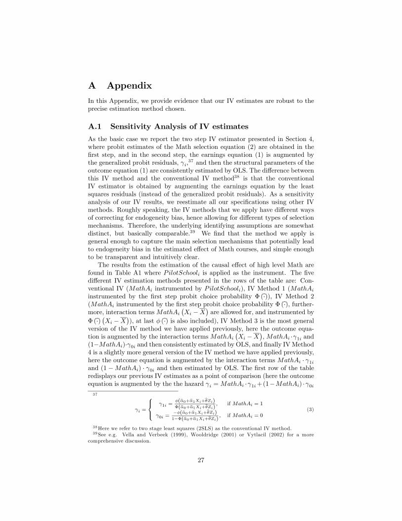
A Appendix

In this Appendix, we provide evidence that our IV estimates are robust to theprecise estimation method chosen.

A.1 Sensitivity Analysis of IV estimates

As the basic case we report the two step IV estimator presented in Section 4,where probit estimates of the Math selection equation (2) are obtained in the�rst step, and in the second step, the earnings equation (1) is augmented bythe generalized probit residuals, i,

37 and then the structural parameters of theoutcome equation (1) are consistently estimated by OLS. The di¤erence betweenthis IV method and the conventional IV method38 is that the conventionalIV estimator is obtained by augmenting the earnings equation by the leastsquares residuals (instead of the generalized probit residuals). As a sensitivityanalysis of our IV results, we reestimate all our speci�cations using other IVmethods. Roughly speaking, the IV methods that we apply have di¤erent waysof correcting for endogeneity bias, hence allowing for di¤erent types of selectionmechanisms. Therefore, the underlying identifying assumptions are somewhatdistinct, but basically comparable.39 We �nd that the method we apply isgeneral enough to capture the main selection mechanisms that potentially leadto endogeneity bias in the estimated e¤ect of Math courses, and simple enoughto be transparent and intuitively clear.The results from the estimation of the causal e¤ect of high level Math are

found in Table A1 where PilotSchooli is applied as the instrument. The �vedi¤erent IV estimation methods presented in the rows of the table are: Con-ventional IV (MathAi instrumented by PilotSchooli), IV Method 1 (MathAiinstrumented by the �rst step probit choice probability � (b�)), IV Method 2(MathAi instrumented by the �rst step probit choice probability � (b�), further-more, interaction termsMathAi

�Xi �X

�are allowed for, and instrumented by

� (b�) �Xi �X�), at last � (b�) is also included), IV Method 3 is the most generalversion of the IV method we have applied previously, here the outcome equa-tion is augmented by the interaction termsMathAi

�Xi �X

�,MathAi � 1i and

(1�MathAi)� 0i and then consistently estimated by OLS, and �nally IVMethod4 is a slightly more general version of the IV method we have applied previously,here the outcome equation is augmented by the interaction terms MathAi � 1iand (1 �MathAi) � 0i and then estimated by OLS. The �rst row of the tableredisplays our previous IV estimates as a point of comparison (here the outcomeequation is augmented by the the hazard i =MathAi � 1i+(1�MathAi) � 0i37

i =

8><>: 1i =

�(b�0+b�1Xi+b�Zi)�(b�0+b�1Xi+b�Zi) ; if MathAi = 1

0i =��(b�0+b�1Xi+b�Zi)1��(b�0+b�1Xi+b�Zi) ; if MathAi = 0

(3)

38Here we refer to two stage least squares (2SLS) as the conventional IV method.39See e.g. Vella and Verbeek (1999), Wooldridge (2001) or Vytlacil (2002) for a more

comprehensive discussion.

27

and estimated by OLS). The conventional IV estimator only allows for restric-tive forms of endogenous selection. Only if the gain from the high level Mathcourse does not vary across individuals, or the expected gain is unobserved tothe individual when choosing the course, the ATEs are identi�ed. IV Method 1requires the same for identi�cation, but is more e¢ cient. Allowing for hetero-geneous gains from Math is notably harder, and this problem has been studiedby e.g. Heckman (1997). Nevertheless, it can be done using either IV Method2 or IV Method 3, where the former is most robust, and the latter relies on anormality assumption for identi�cation.40 Furthermore, IV Method 2 allows usto separate the issue of endogenous and nonconstant treatment e¤ects by testingthe signi�cance of the coe¢ cient on � (b�). We �nd that it is only signi�cant inthe speci�cations where we control for the level-subject categories of higher ed-ucation, i.e. nonconstant treatment e¤ects only seem important given subjectof postsecondary education. Hence, the gains that high school graduates getfrom the high level Math course depend on the chosen subject of postsecondaryeducation. This is also consistent with what we deduced from our results inSection 6. One advantage of IV Methods 3 and 4 (and also the one we apply)is, however, that they estimate a number of additional parameters that provideus with information about the self-selection mechanism. The results from IVMethod 2 deviate most from our previous results as the e¤ect of Math is notalways found to be signi�cantly larger than zero. It should be noted, however,that IV Method 2 may not be well speci�ed in our settings due to collinearityissues. Not surprisingly, IV Method 4 gives estimates closest to the ones wepreviously found. Overall, it is reassuring that our main conclusions regardingthe causal e¤ects do not change signi�cantly depending on the particular IVestimation method chosen.

B Appendix

In this Appendix, we provide tests of the validity of the instruments, selectione¤ects and heterogeneous treatment e¤ects.

B.1 Testing Validity of Instruments

In this section, we corroborate that PilotSchool is a valid instrument. First,we examine whether the pilot schools di¤er in systematic ways from non-pilotschools. This is done by comparing the observable characteristics of the highschool graduates and their parents. Second, we attempt to estimate the impliedbias in the causal e¤ect by looking at the e¤ect of PilotSchooli for high schoolgraduates with language based studies for which the advanced Math course isnot a serious option.

40One might say that it is a trade-o¤ between non-normality against robustness and e¢ -ciency.

28

B.1.1 Comparing the pilot schools to non-pilot schools

If individuals are randomly assigned to pilot schools because of exogenous vari-ation due to place of residence and preferences for other school characteristics,any observed di¤erences would solely be attributed to the fact that choices ofhigh school Math courses di¤er between the two cohorts. However, if thereare systematic and signi�cant di¤erences between observable characteristics ofthe two high school cohorts before they start high school, one might questionthat the two cohorts have similar distributions of unobservable labor marketand math abilities. Therefore, we compare the primary school attendance andparental background variables of the two high school cohorts before high schoolentry. The descriptive statistics in Table 1 do not give us any reason to believethat the students at the pilot schools di¤er in any respect from those at the non-pilot schools. In other words, students seem fairly randomly distributed acrosspilot and non-pilot schools that do and do not o¤er experimental curriculumwith advanced Math.We also look closely at the characteristics of students at pilot schools versus

non-pilot schools after 1988 when the pilot scheme was no longer in action. We�nd no observed di¤erences.

B.1.2 Implied Bias of IV estimates

Now we try to directly estimate the implied bias in the estimated causal e¤ects.Following Altonji, Elder and Taber (2004), who evaluate IV estimation strategiesfor estimating the e¤ects of Catholic schooling, we identify a sample of individu-als for whom the high level Math course is not a serious option. Hence, we takeadvantage of the fact that the high school students who, upon high school entry,choose the language track have zero probability of attending the high level Mathcourse, see Figure 2. LetMi be an indicator variable equal to one if individual ichooses Math track (Mi = 1), and equal to zero if i chooses the language track(Mi = 0) upon high school entry. Then P (MathAi = 1jMi = 0) = 0. Fur-thermore, we assume that the joint distribution of (Xi; Zi; "i) is independent ofMi.41

It is well known that the conventional IV estimate of the causal e¤ect of highlevel Math on earnings, �, converges to:

�IVp! � +

cov�fZi; "i�

�V ar�fZi� ;

41The descriptives in Table 1 reveal that changes in the self-selection mechanism of studentsbetween math and language tracks might be induced by the pilot scheme as 34% of the studentsat non-pilot schools and 30% pilot schools choose the language track. However, since thesedi¤erences are similar in the post-reform cohorts entering high school in 1988 and 1989, theredoes not seem to arise a potential selection problem by restricting the analysis to the sample ofhigh school graduates from the language track, and we do not account for potential correlationbetween Zi and "i, induced by conditioning on Mi.

29

where fZi is the residual from the projection of Zi on Xi. Since we have aconsistent estimate of � from the �rst stage estimation, a consistent estimate of

the bias, � =cov(fZi;"i)�V ar(fZi) ; can be obtained by estimating the equation:

yi;13 = �1Xi +�b�Zi� � + vi;

by OLS on the sample of high school graduates from the language track. Theparameter estimate of � is then a consistent estimate of the implied bias.Table B1 shows the estimated biases along with the estimated IV coe¢ cients

as a point of reference. The bias tends to be positive for PilotSchool, however,insigni�cant in all speci�cations. This indicates that the positive causal e¤ectof advanced Math for the students who are induced to choose advanced Mathcombined with Chemistry can be considered an upper bound. Since all the im-plied biases are statistically insigni�cant, we are con�dent that our instrument,PilotSchool; is indeed a proper instrument.

B.2 Tests of Homogeneity Assumptions

In this section, we corroborate the validity of the pilot scheme based instru-ments as a basis for extrapolation. The analysis in the preceding subsection hasestablished that the reform based instruments estimate internally valid causale¤ects. However, in order to make inference for other populations, the causale¤ects have to satisfy some additional homogeneity assumptions in order forLATE to equal ATE. In this subsection, we test two of these assumptions:42

First of all, if there was no selection bias (or equivalently constant e¤ects), thenof course LATE would equal ATE and ATT. The assumption of no selectionbias can be tested by the Durbin-Wu-Hausman (DWH) test which is equivalentto the more e¢ cient test proposed by Angrist (2004) under the monotonicityassumption. The tests show that the hypothesis of no selection bias does notseem credible in our application.The second homogeneity assumption is that of conditional constant e¤ects,

which allows for selection bias in the sense that Y1i and Y0i are allowed to becorrelated with potential participation in the advanced Math course. However,Y1i � Y0i is orthogonal to potential participation, i.e. it is restricted to be thesame for both potential outcomes. This assumption is consistent with absoluteadvantage, but rules out comparative advantage, i.e. Roy (1951) type of se-lection, where the choice of the advanced Math course is determined by thepotential gains from completing the course. Hence, the conditional constante¤ect assumption implies that the ATE is the same, regardless of a student�slikelihood of choosing advanced Math. Since the ATE (by de�nition) is invari-ant to the particular instrument applied to estimate it, the underlying idea ofthe test is to compare the estimated ATEs using di¤erent instruments. Underthe assumption of conditional constant e¤ects, this test amounts to a Sargan

42A more comprehensive description of homogeneity assumptions and tests can be found ine.g. Angrist (2004) and Baum, Scha¤er and Stillman (2003).

30

(1958) test for over-identi�cation. The drawback of this test is that it can onlybe applied if we have more excluded instruments than endogenous control vari-ables, and that it tests for the failure of any of the instruments to satisfy theorthogonality conditions. In the case of the pre-reform cohorts, we can more re-liably employ a "di¤erence-in-Sargan" test statistic, which in e¤ect is computedas the di¤erence between two Sargan test statistics (that for the regressionusing the entire set of overidentifying restrictions, and that for the regressionusing a smaller set of restrictions from which a speci�ed instrument is removed).Hence, it allows us to test that the speci�ed instrumental variable satis�es theorthogonality condition. This test can only reject the conditional constant e¤ectassumption for PilotSchool in the speci�cation without any exogenous controlvariables with a p-value of 0.008. For all other speci�cations, the hypothesisthat PilotSchool satis�es the orthogonality condition cannot be rejected at anyusual levels of signi�cance (all p-values>0.667). Similarly, for DistP ilotSchool,the hypothesis cannot be rejected for any speci�cation (all p-values>0.19). Toconclude, we do not �nd any reason to doubt the conditional constant e¤ectassumption, and accordingly, we believe that we can trust extrapolations ofATEs estimated by instruments PilotSchool and DistP ilotSchool. Note thatthe symmetry assumption discussed in Section 6.1.3 implies a less restrictivehomogeneity assumption than the assumption of conditional constant e¤ects,namely, that the conditional expectation of the potential outcomes is a linearfunction of MathA0i +MathA1i.

31

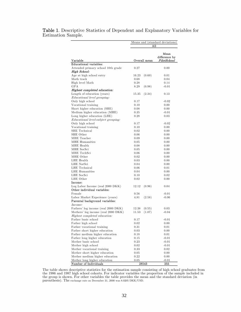
32

Table 1. Descriptive Statistics of Dependent and Explanatory Variables for Estimation Sample.

Variable

Mean difference by PilotSchool

Educational variables:Attended primary school 10th grade 0.27 0.00High School:Age at high school entry 16.23 (0.60) 0.01Math track 0.68 0.04High level Math 0.28 0.14GPA 8.29 (0.98) -0.01Highest completed education:Length of education (years) 15.35 (2.34) 0.13Educational level grouping:Only high school 0.17 -0.02Vocational training 0.10 0.00Short higher education (SHE) 0.08 0.00Medium higher education (MHE) 0.35 -0.01Long higher education (LHE) 0.28 0.03Educational level-subject grouping:Only high school 0.17 -0.02Vocational training 0.10 0.00SHE Technical 0.02 0.00SHE Other 0.06 0.00MHE Teacher 0.09 0.00MHE Humanities 0.05 0.00MHE Health 0.08 0.00MHE SocSci 0.05 0.00MHE TechSci 0.06 0.00MHE Other 0.02 0.00LHE Health 0.03 0.00LHE NatSci 0.04 0.00LHE Technical 0.06 0.01LHE Humanities 0.04 0.00LHE SocSci 0.10 0.02LHE Other 0.02 0.00Income:Log Labor Income (real 2000 DKK) 12.12 (0.96) 0.04Other individual variables:Female 0.56 -0.01Labor Market Experience (years) 4.81 (2.58) -0.06Parental background variables:Income:Fathers’ log income (real 2000 DKK) 12.38 (0.55) 0.03Mothers’ log income (real 2000 DKK) 11.53 (1.07) -0.04Highest completed education:Father basic school 0.17 -0.01Father high school 0.02 0.00Father vocational training 0.31 0.01Father short higher education 0.03 0.00Father medium higher education 0.18 0.01Father long higher education 0.15 -0.01Mother basic school 0.23 -0.01Mother high school 0.02 -0.01Mother vocational training 0.33 0.02Mother short higher education 0.05 0.00Mother medium higher education 0.22 0.00Mother long higher education 0.05 -0.01Number of Individuals 25528543

Overall mean

AllMeans and (standard deviations)

The table shows descriptive statistics for the estimation sample consisting of high school graduates from the 1986 and 1987 high school cohorts. For indicator variables the proportion of the sample included in the group is shown. For other variables the table provides the mean and the standard deviation (in parenthesis). The exchange rate on December 31, 2000 was 8.0205 DKK/USD.

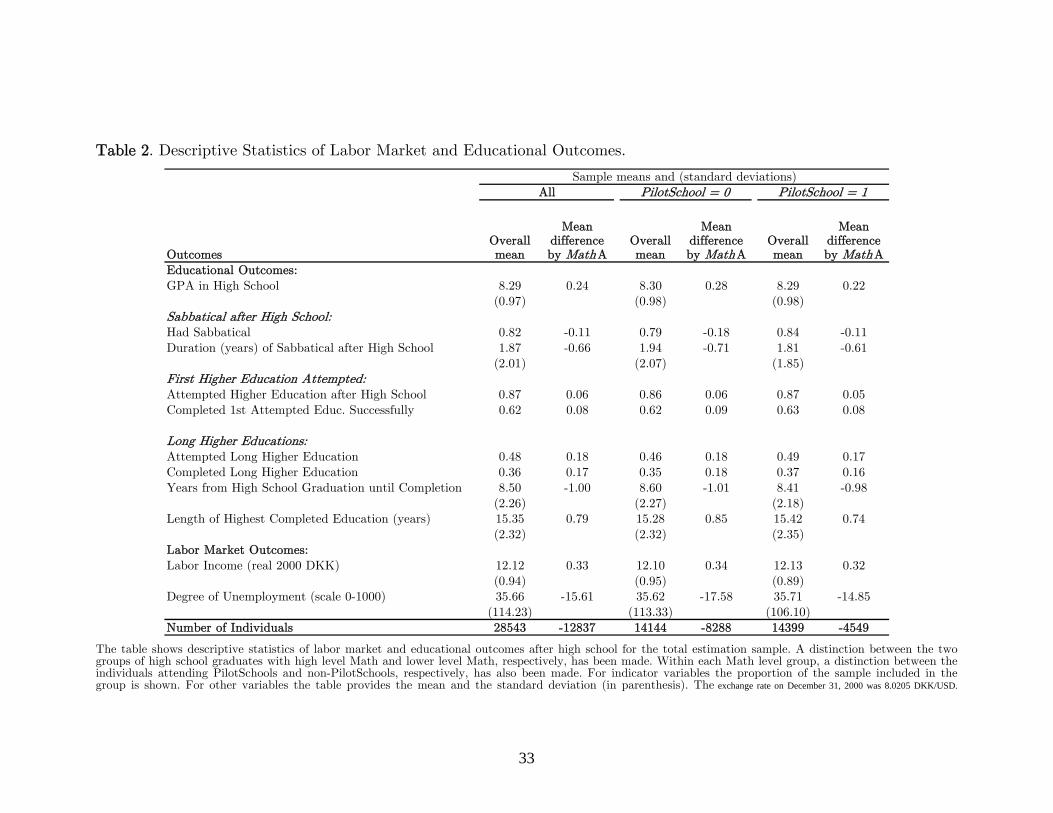
33

Table 2. Descriptive Statistics of Labor Market and Educational Outcomes.

OutcomesOverall mean

Mean difference by MathA

Overall mean

Mean difference by MathA

Overall mean

Mean difference by MathA

Educational Outcomes:GPA in High School 8.29 0.24 8.30 0.28 8.29 0.22

(0.97) (0.98) (0.98)Sabbatical after High School:Had Sabbatical 0.82 -0.11 0.79 -0.18 0.84 -0.11Duration (years) of Sabbatical after High School 1.87 -0.66 1.94 -0.71 1.81 -0.61

(2.01) (2.07) (1.85)First Higher Education Attempted:Attempted Higher Education after High School 0.87 0.06 0.86 0.06 0.87 0.05Completed 1st Attempted Educ. Successfully 0.62 0.08 0.62 0.09 0.63 0.08

Long Higher Educations:Attempted Long Higher Education 0.48 0.18 0.46 0.18 0.49 0.17Completed Long Higher Education 0.36 0.17 0.35 0.18 0.37 0.16Years from High School Graduation until Completion 8.50 -1.00 8.60 -1.01 8.41 -0.98

(2.26) (2.27) (2.18)Length of Highest Completed Education (years) 15.35 0.79 15.28 0.85 15.42 0.74

(2.32) (2.32) (2.35)Labor Market Outcomes:Labor Income (real 2000 DKK) 12.12 0.33 12.10 0.34 12.13 0.32

(0.94) (0.95) (0.89)Degree of Unemployment (scale 0-1000) 35.66 -15.61 35.62 -17.58 35.71 -14.85

(114.23) (113.33) (106.10)Number of Individuals 28543 -12837 14144 -8288 14399 -4549

PilotSchool = 1AllSample means and (standard deviations)

PilotSchool = 0

The table shows descriptive statistics of labor market and educational outcomes after high school for the total estimation sample. A distinction between the two groups of high school graduates with high level Math and lower level Math, respectively, has been made. Within each Math level group, a distinction between the individuals attending PilotSchools and non-PilotSchools, respectively, has also been made. For indicator variables the proportion of the sample included in the group is shown. For other variables the table provides the mean and the standard deviation (in parenthesis). The exchange rate on December 31, 2000 was 8.0205 DKK/USD.

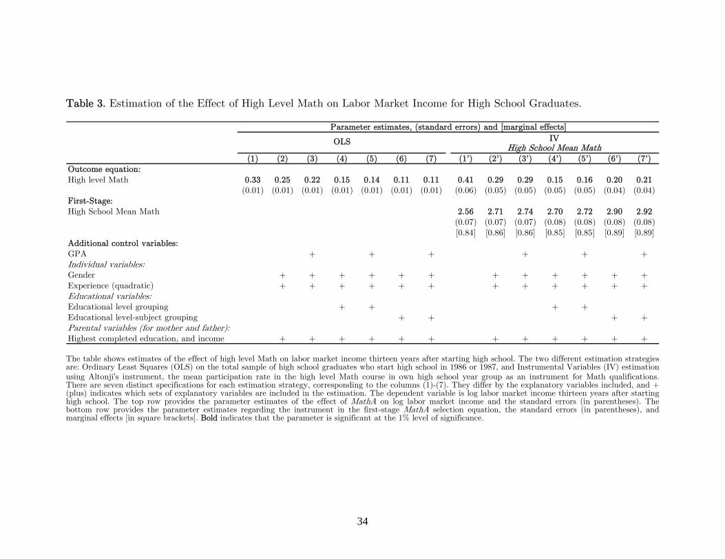
34

Table 3. Estimation of the Effect of High Level Math on Labor Market Income for High School Graduates.

(1) (2) (3) (4) (5) (6) (7) (1’) (2’) (3’) (4’) (5’) (6’) (7’)Outcome equation:High level Math 0.33 0.25 0.22 0.15 0.14 0.11 0.11 0.41 0.29 0.29 0.15 0.16 0.20 0.21

(0.01) (0.01) (0.01) (0.01) (0.01) (0.01) (0.01) (0.06) (0.05) (0.05) (0.05) (0.05) (0.04) (0.04)First-Stage:High School Mean Math 2.56 2.71 2.74 2.70 2.72 2.90 2.92

(0.07) (0.07) (0.07) (0.08) (0.08) (0.08) (0.08)[0.84] [0.86] [0.86] [0.85] [0.85] [0.89] [0.89]

Additional control variables:GPA + + + + + +Individual variables:Gender + + + + + + + + + + + +Experience (quadratic) + + + + + + + + + + + +Educational variables:Educational level grouping + + + +Educational level-subject grouping + + + +Parental variables (for mother and father):Highest completed education, and income + + + + + + + + + + + +

OLS

Parameter estimates, (standard errors) and [marginal effects]

IV High School Mean Math

The table shows estimates of the effect of high level Math on labor market income thirteen years after starting high school. The two different estimation strategies are: Ordinary Least Squares (OLS) on the total sample of high school graduates who start high school in 1986 or 1987, and Instrumental Variables (IV) estimation using Altonji’s instrument, the mean participation rate in the high level Math course in own high school year group as an instrument for Math qualifications. There are seven distinct specifications for each estimation strategy, corresponding to the columns (1)-(7). They differ by the explanatory variables included, and + (plus) indicates which sets of explanatory variables are included in the estimation. The dependent variable is log labor market income thirteen years after starting high school. The top row provides the parameter estimates of the effect of MathA on log labor market income and the standard errors (in parentheses). The bottom row provides the parameter estimates regarding the instrument in the first-stage MathA selection equation, the standard errors (in parentheses), and marginal effects [in square brackets]. Bold indicates that the parameter is significant at the 1% level of significance.

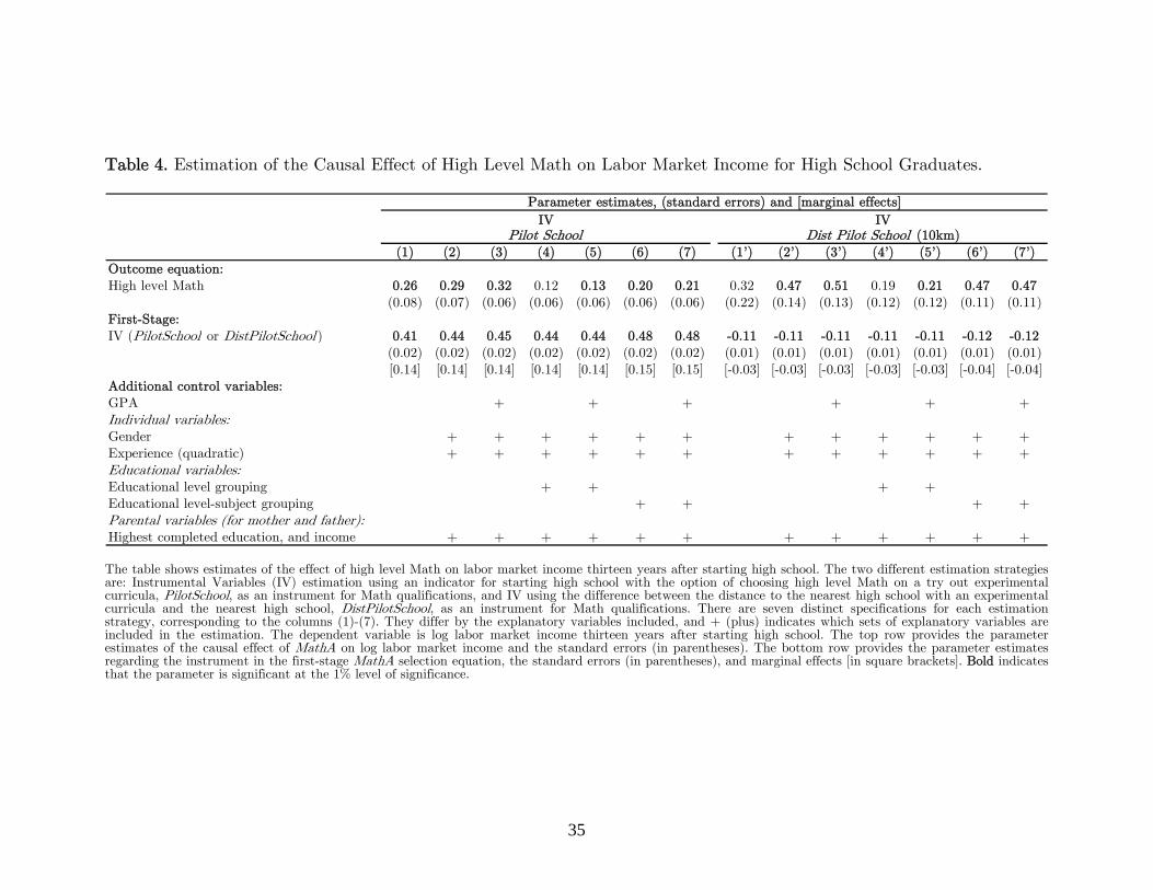
35

Table 4. Estimation of the Causal Effect of High Level Math on Labor Market Income for High School Graduates.

(1) (2) (3) (4) (5) (6) (7) (1’) (2’) (3’) (4’) (5’) (6’) (7’)Outcome equation:High level Math 0.26 0.29 0.32 0.12 0.13 0.20 0.21 0.32 0.47 0.51 0.19 0.21 0.47 0.47

(0.08) (0.07) (0.06) (0.06) (0.06) (0.06) (0.06) (0.22) (0.14) (0.13) (0.12) (0.12) (0.11) (0.11)First-Stage:IV (PilotSchool or DistPilotSchool ) 0.41 0.44 0.45 0.44 0.44 0.48 0.48 -0.11 -0.11 -0.11 -0.11 -0.11 -0.12 -0.12

(0.02) (0.02) (0.02) (0.02) (0.02) (0.02) (0.02) (0.01) (0.01) (0.01) (0.01) (0.01) (0.01) (0.01)[0.14] [0.14] [0.14] [0.14] [0.14] [0.15] [0.15] [-0.03] [-0.03] [-0.03] [-0.03] [-0.03] [-0.04] [-0.04]

Additional control variables:GPA + + + + + +Individual variables:Gender + + + + + + + + + + + +Experience (quadratic) + + + + + + + + + + + +Educational variables:Educational level grouping + + + +Educational level-subject grouping + + + +Parental variables (for mother and father):Highest completed education, and income + + + + + + + + + + + +

Parameter estimates, (standard errors) and [marginal effects]

IV Pilot School

IV Dist Pilot School (10km)

The table shows estimates of the effect of high level Math on labor market income thirteen years after starting high school. The two different estimation strategies are: Instrumental Variables (IV) estimation using an indicator for starting high school with the option of choosing high level Math on a try out experimental curricula, PilotSchool, as an instrument for Math qualifications, and IV using the difference between the distance to the nearest high school with an experimental curricula and the nearest high school, DistPilotSchool, as an instrument for Math qualifications. There are seven distinct specifications for each estimation strategy, corresponding to the columns (1)-(7). They differ by the explanatory variables included, and + (plus) indicates which sets of explanatory variables are included in the estimation. The dependent variable is log labor market income thirteen years after starting high school. The top row provides the parameter estimates of the causal effect of MathA on log labor market income and the standard errors (in parentheses). The bottom row provides the parameter estimates regarding the instrument in the first-stage MathA selection equation, the standard errors (in parentheses), and marginal effects [in square brackets]. Bold indicates that the parameter is significant at the 1% level of significance.

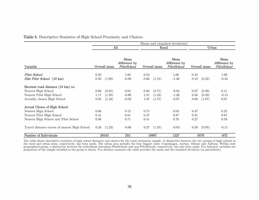
36

Table 5. Descriptive Statistics of High School Proximity and Choices.

Variable

Mean difference by PilotSchool

Mean difference by PilotSchool

Mean difference by PilotSchool

Pilot School 0.50 1.00 0.53 1.00 0.45 1.00Dist Pilot School (10 km) 0.50 (1.00) -0.90 0.66 (1.18) -1.30 0.19 (0.32) -0.24

Shortest road distance (10 km) to:Nearest High School 0.66 (0.65) 0.04 0.80 (0.71) -0.04 0.37 (0.39) 0.11Nearest Pilot High School 1.17 (1.20) -0.86 1.47 (1.33) -1.36 0.56 (0.49) -0.13Actually chosen High School 0.94 (1.43) -0.02 1.07 (1.57) -0.07 0.68 (1.07) 0.01

Actual Choice of High School:Nearest High School 0.66 0.12 0.75 0.03 0.47 0.22Nearest Pilot High School 0.41 0.81 0.47 0.87 0.31 0.67Nearest High School and Pilot School 0.36 0.71 0.41 0.76 0.27 0.59

Travel distance excess of nearest High School 0.28 (1.23) -0.06 0.27 (1.35) -0.03 0.30 (0.95) -0.11

Number of Individuals 255 1227 -972

Means and (standard deviations)All Rural Urban

Overall mean Overall mean Overall mean

28543 18967 9576 The table shows descriptive statistics of high school distances and choices for the total estimation sample. A distinction between the two groups of high schools in the rural and urban areas, respectively, has been made. The urban area includes the four biggest cities: Copenhagen, Aarhus, Odense and Aalborg. Within each geographical group, a distinction between the individuals attending PilotSchools and non-PilotSchools, respectively, has also been made. For indicator variables the proportion of the sample included in the group is shown. For distance measures the table provides the mean and the standard deviation (in parenthesis).

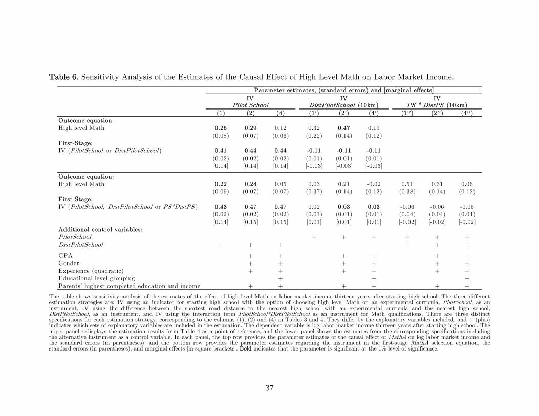
37

Table 6. Sensitivity Analysis of the Estimates of the Causal Effect of High Level Math on Labor Market Income.

(1) (2) (4) (1’) (2’) (4’) (1’’) (2’’) (4’’)Outcome equation:High level Math 0.26 0.29 0.12 0.32 0.47 0.19

(0.08) (0.07) (0.06) (0.22) (0.14) (0.12)First-Stage:IV (PilotSchool or DistPilotSchool ) 0.41 0.44 0.44 -0.11 -0.11 -0.11

(0.02) (0.02) (0.02) (0.01) (0.01) (0.01)[0.14] [0.14] [0.14] [-0.03] [-0.03] [-0.03]

Outcome equation:High level Math 0.22 0.24 0.05 0.03 0.21 -0.02 0.51 0.31 0.06

(0.09) (0.07) (0.07) (0.37) (0.14) (0.12) (0.38) (0.14) (0.12)First-Stage:IV (PilotSchool, DistPilotSchool or PS*DistPS ) 0.43 0.47 0.47 0.02 0.03 0.03 -0.06 -0.06 -0.05

(0.02) (0.02) (0.02) (0.01) (0.01) (0.01) (0.04) (0.04) (0.04)[0.14] [0.15] [0.15] [0.01] [0.01] [0.01] [-0.02] [-0.02] [-0.02]

Additional control variables:PilotSchool + + + + + +DistPilotSchool + + + + + +

GPA + + + + + +Gender + + + + + +Experience (quadratic) + + + + + +Educational level grouping + + +Parents’ highest completed education and income + + + + + +

Parameter estimates, (standard errors) and [marginal effects]

IV PS * DistPS (10km)

IV Pilot School

IV DistPilotSchool (10km)

The table shows sensitivity analysis of the estimates of the effect of high level Math on labor market income thirteen years after starting high school. The three different estimation strategies are: IV using an indicator for starting high school with the option of choosing high level Math on an experimental curricula, PilotSchool, as an instrument, IV using the difference between the shortest road distance to the nearest high school with an experimental curricula and the nearest high school, DistPilotSchool, as an instrument, and IV using the interaction term PilotSchool*DistPilotSchool as an instrument for Math qualifications. There are three distinct specifications for each estimation strategy, corresponding to the columns (1), (2) and (4) in Tables 3 and 4. They differ by the explanatory variables included, and + (plus) indicates which sets of explanatory variables are included in the estimation. The dependent variable is log labor market income thirteen years after starting high school. The upper panel redisplays the estimation results from Table 4 as a point of reference, and the lower panel shows the estimates from the corresponding specifications including the alternative instrument as a control variable. In each panel, the top row provides the parameter estimates of the causal effect of MathA on log labor market income and the standard errors (in parentheses), and the bottom row provides the parameter estimates regarding the instrument in the first-stage MathA selection equation, the standard errors (in parentheses), and marginal effects [in square brackets]. Bold indicates that the parameter is significant at the 1% level of significance.

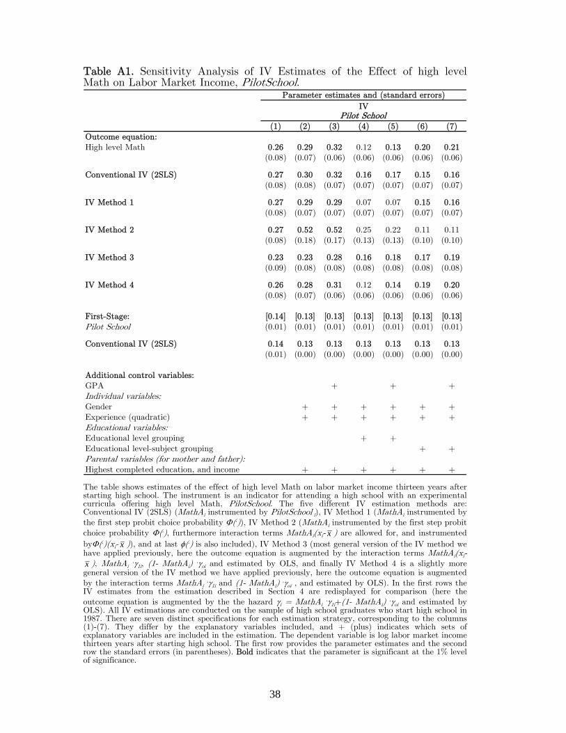
38

Table A1. Sensitivity Analysis of IV Estimates of the Effect of high level Math on Labor Market Income, PilotSchool.

(1) (2) (3) (4) (5) (6) (7)Outcome equation:High level Math 0.26 0.29 0.32 0.12 0.13 0.20 0.21

(0.08) (0.07) (0.06) (0.06) (0.06) (0.06) (0.06)

Conventional IV (2SLS) 0.27 0.30 0.32 0.16 0.17 0.15 0.16(0.08) (0.08) (0.07) (0.07) (0.07) (0.07) (0.07)

IV Method 1 0.27 0.29 0.29 0.07 0.07 0.15 0.16(0.08) (0.07) (0.07) (0.07) (0.07) (0.07) (0.07)

IV Method 2 0.27 0.52 0.52 0.25 0.22 0.11 0.11(0.08) (0.18) (0.17) (0.13) (0.13) (0.10) (0.10)

IV Method 3 0.23 0.23 0.28 0.16 0.18 0.17 0.19(0.09) (0.08) (0.08) (0.08) (0.08) (0.08) (0.08)

IV Method 4 0.26 0.28 0.31 0.12 0.14 0.19 0.20(0.08) (0.07) (0.06) (0.06) (0.06) (0.06) (0.06)

First-Stage: [0.14] [0.13] [0.13] [0.13] [0.13] [0.13] [0.13]Pilot School (0.01) (0.01) (0.01) (0.01) (0.01) (0.01) (0.01)

Conventional IV (2SLS) 0.14 0.13 0.13 0.13 0.13 0.13 0.13(0.01) (0.00) (0.00) (0.00) (0.00) (0.00) (0.00)

Additional control variables:GPA + + +Individual variables:Gender + + + + + +Experience (quadratic) + + + + + +Educational variables:Educational level grouping + +Educational level-subject grouping + +Parental variables (for mother and father):Highest completed education, and income + + + + + +

IV Pilot School

Parameter estimates and (standard errors)

The table shows estimates of the effect of high level Math on labor market income thirteen years after starting high school. The instrument is an indicator for attending a high school with an experimental curricula offering high level Math, PilotSchool. The five different IV estimation methods are: Conventional IV (2SLS) (MathAi instrumented by PilotSchool i), IV Method 1 (MathAi instrumented by

the first step probit choice probability Φ(.)), IV Method 2 (MathAi instrumented by the first step probit

choice probability Φ(.), furthermore interaction terms MathAi(xi- x ) are allowed for, and instrumented

byΦ(.)(xi- x )), and at last φ(.) is also included), IV Method 3 (most general version of the IV method we have applied previously, here the outcome equation is augmented by the interaction terms MathAi(xi-

x ), MathAi .γ1i, (1- MathAi)

.γoi and estimated by OLS, and finally IV Method 4 is a slightly more general version of the IV method we have applied previously, here the outcome equation is augmented

by the interaction terms MathAi .γ1i and (1- MathAi)

.γoi , and estimated by OLS). In the first rows the IV estimates from the estimation described in Section 4 are redisplayed for comparison (here the

outcome equation is augmented by the the hazard γi = MathAi .γ1i+(1- MathAi)

.γoi and estimated by OLS). All IV estimations are conducted on the sample of high school graduates who start high school in 1987. There are seven distinct specifications for each estimation strategy, corresponding to the columns (1)-(7). They differ by the explanatory variables included, and + (plus) indicates which sets of explanatory variables are included in the estimation. The dependent variable is log labor market income thirteen years after starting high school. The first row provides the parameter estimates and the second row the standard errors (in parentheses). Bold indicates that the parameter is significant at the 1% level of significance.

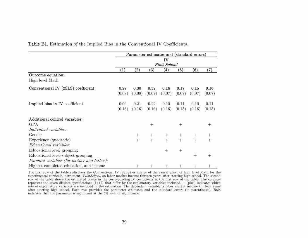
39

Table B1. Estimation of the Implied Bias in the Conventional IV Coefficients.

(1) (2) (3) (4) (5) (6) (7)Outcome equation:High level Math

Conventional IV (2SLS) coefficient 0.27 0.30 0.32 0.16 0.17 0.15 0.16(0.08) (0.08) (0.07) (0.07) (0.07) (0.07) (0.07)

Implied bias in IV coefficient 0.06 0.21 0.22 0.10 0.11 0.10 0.11(0.16) (0.16) (0.16) (0.16) (0.15) (0.16) (0.15)

Additional control variables:GPA + + +Individual variables:Gender + + + + + +Experience (quadratic) + + + + + +Educational variables:Educational level grouping + +Educational level-subject grouping + +Parental variables (for mother and father):Highest completed education, and income + + + + + +

IV Pilot School

Parameter estimates and (standard errors)

The first row of the table redisplays the Conventional IV (2SLS) estimates of the causal effect of high level Math for the experimental curricula instrument, PilotSchool, on labor market income thirteen years after starting high school. The second row of the table shows the estimated biases in the corresponding IV coefficients in the first row of the table. The columns represent the seven distinct specifications (1)-(7) that differ by the explanatory variables included. + (plus) indicates which sets of explanatory variables are included in the estimation. The dependent variable is labor market income thirteen years after starting high school. Each row provides the parameter estimates and the standard errors (in parentheses). Bold indicates that the parameter is significant at the 5% level of significance.

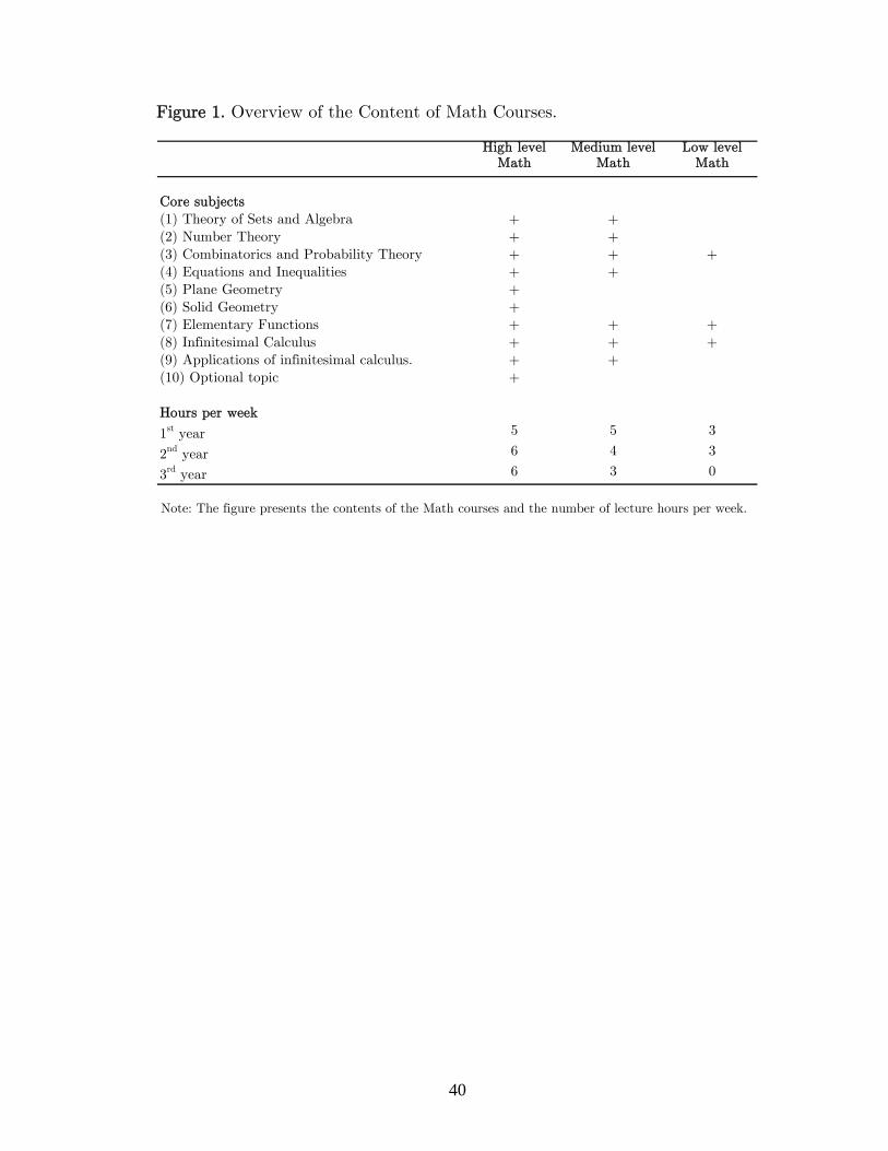
40

Figure 1. Overview of the Content of Math Courses.

High level Math

Medium level Math

Low level Math

Core subjects(1) Theory of Sets and Algebra + +

(2) Number Theory + +

(3) Combinatorics and Probability Theory + + +(4) Equations and Inequalities + +

(5) Plane Geometry +

(6) Solid Geometry +(7) Elementary Functions + + +

(8) Infinitesimal Calculus + + +

(9) Applications of infinitesimal calculus. + +(10) Optional topic +

Hours per week

1st year 5 5 3

2nd year 6 4 3

3rd year 6 3 0 Note: The figure presents the contents of the Math courses and the number of lecture hours per week.

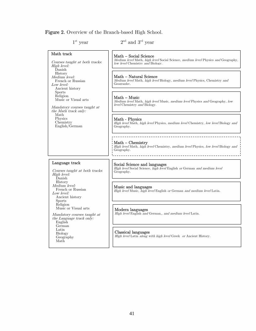
41

Figure 2. Overview of the Branch-based High School.

1st year 2nd and 3rd year

Math – Social Science Medium level Math, high level Social Science, medium level Physics and Geography, low level Chemistry and Biology.

Math track Courses taught at both tracks: High level: Danish History Medium level: French or Russian Low level: Ancient history Sports Religion Music or Visual arts Mandatory courses taught at the Math track only: Math Physics Chemistry English/German

Language track Courses taught at both tracks: High level: Danish History Medium level: French or Russian Low level: Ancient history Sports Religion Music or Visual arts

Mandatory courses taught at the Language track only: English German Latin Biology Geography Math

Math – Natural Science Medium level Math, high level Biology, medium level Physics, Chemistry and Geography,

Math – Music Medium level Math, high level Music, medium level Physics and Geography, low level Chemistry and Biology.

Math – Chemistry High level Math, high level Chemistry, medium level Physics, low level Biology and Geography.

Modern languagesHigh level English and German,, and medium level Latin.

Music and languagesHigh level Music, high level English or German and medium level Latin.

Social Science and languagesHigh level Social Science, high level English or German and medium level Geography.

Math - PhysicsHigh level Math, high level Physics, medium level Chemistry, low level Biology and Geography.

Classical languagesHigh level Latin along with high level Greek or Ancient History.

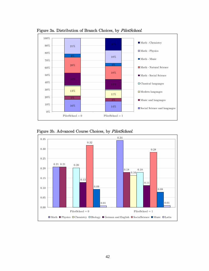
42

Figure 3a. Distribution of Branch Choices, by PilotSchool.

16% 14%

5%4%

13%11%

16%

14%

20%

18%

4%

4%

21%

18%

16%

0%

10%

20%

30%

40%

50%

60%

70%

80%

90%

100%

PilotSchool = 0 PilotSchool = 1

Math - Chemistry

Math - Physics

Math - Music

Math - Natural Science

Math - Social Science

Classical languages

Modern languages

Music and languages

Social Science and languages

Figure 3b. Advanced Course Choices, by PilotSchool.

0.21

0.34

0.21

0.180.16

0.20

0.18

0.130.11

0.32

0.28

0.090.08

0.01 0.01

0.00

0.05

0.10

0.15

0.20

0.25

0.30

0.35

PilotSchool = 0 PilotSchool = 1

Math Physics Chemistry Biology German and English SocialScience Music Latin