Policy Research Working Paper 6346

Is Foreign Aid Fungible?

Evidence from the Education and Health Sectors

Nicolas Van de Sijpe

The World BankDevelopment Economics Vice PresidencyPartnerships, Capacity Building UnitJanuary 2013

WPS6346P

ublic

Dis

clos

ure

Aut

horiz

edP

ublic

Dis

clos

ure

Aut

horiz

edP

ublic

Dis

clos

ure

Aut

horiz

edP

ublic

Dis

clos

ure

Aut

horiz

edP

ublic

Dis

clos

ure

Aut

horiz

edP

ublic

Dis

clos

ure

Aut

horiz

edP

ublic

Dis

clos

ure

Aut

horiz

edP

ublic

Dis

clos

ure

Aut

horiz

ed

Produced by the Research Support Team

Abstract

The Policy Research Working Paper Series disseminates the findings of work in progress to encourage the exchange of ideas about development issues. An objective of the series is to get the findings out quickly, even if the presentations are less than fully polished. The papers carry the names of the authors and should be cited accordingly. The findings, interpretations, and conclusions expressed in this paper are entirely those of the authors. They do not necessarily represent the views of the International Bank for Reconstruction and Development/World Bank and its affiliated organizations, or those of the Executive Directors of the World Bank or the governments they represent.

Policy Research Working Paper 6346

This paper adopts a new approach to the issue of foreign aid fungibility. In contrast to most existing empirical studies, panel data are employed that contain information on the specific purposes for which aid is given. This allows linking aid that is provided for education and health purposes to recipient public spending in these sectors. In addition, aid flows that are recorded on a recipient’s budget are distinguished from those that are not recorded on budget, and the previous failure to differentiate between on- and off-budget aid is shown to

This paper is a product of the Partnerships, Capacity Building Unit, Development Economics Vice Presidency. It is part of a larger effort by the World Bank to provide open access to its research and make a contribution to development policy discussions around the world. Policy Research Working Papers are also posted on the Web at http://econ.worldbank.org. The author may be contacted at nicolas.vandesijpe@qeh.ox.ac.uk.

produce biased estimates of fungibility. Sector program aid is the measure of on-budget aid, whereas technical cooperation serves as a proxy for off-budget aid. The appropriate treatment of off-budget aid leads to lower fungibility estimates than those reported in many previous studies. Specifically, in both sectors and across a range of specifications, technical cooperation, which is the largest component of total education and health aid, leads to, at most, a small displacement of recipient public expenditures.

Is foreign aid fungible? Evidence from the education and health

sectors

Nicolas Van de Sijpe∗

Keywords: foreign aid, fungibility, public education expenditure, public health expenditure.

JEL classification codes: E62, F35, H50, O23.

Sector Board: Economic Policy (EPOL).∗Departmental Lecturer in Development Economics, Department of International Development, and Research Associate, Cen-

tre for the Study of African Economies (CSAE), University of Oxford. Address: Queen Elizabeth House, 3 Mansfield Road, Ox-ford, OX1 3TB, United Kingdom. E-mail: nicolas.vandesijpe@qeh.ox.ac.uk. I am grateful to Sudhir Anand, Channing Arndt, SteveBond, Maarten Bosker, Paolo de Renzio, Markus Eberhardt, Bernard Gauthier, Benedikt Goderis, Clare Leaver, Anita Ratcliffe, MansSoderbom, Francis Teal, Dirk Van de Gaer, David Vines, John Wilson, the participants at various conferences and seminars, and es-pecially Chris Adam, Paul Collier, Shanta Devarajan, Jon Temple, Frank Windmeijer, Adrian Wood and three anonymous referees foruseful comments and discussions. I am also grateful to Ali Abbas, Nicolas Depetris Chauvin, Ibrahim Levent and Gerd Schwartz forassistance in obtaining data. I would like to thank the people at the OECD Development Assistance Committee (DAC), especiallyCecile Sangare, for patiently answering my questions about their development assistance data and Brian Hammond for comments onthe aid data construction. I gratefully acknowledge funding from the Department of Economics, the Oxford Centre for the Analysis ofResource Rich Economies (OxCarre), the Oxford Institute for Global Economic Development (OxIGED) and St. Catherine’s College,University of Oxford. This paper presents the research results of the Belgian Programme on Interuniversity Poles of Attraction (contractno. P6/07) initiated by the Belgian State, Prime Minister’s Office, Science Policy Programming.

The effect of foreign aid on economic growth, poverty, and developmental outcomes may depend heavily

on the fiscal response of recipient governments. One aspect of this fiscal response is the possibility that aid may

be fungible (i.e., the net effect of earmarked aid differs from the intended effect).

This paper endeavors to determine the extent to which earmarked education and health aid are fungible.

Many studies of foreign aid fungibility are hampered by a lack of comprehensive data pertaining to the in-

tended purpose of aid. I use the OECD’s Creditor Reporting System (CRS), which disaggregates aid by sector,

to overcome this problem. To cope with the incompleteness of the CRS data, I propose a novel data construc-

tion method that begins with the CRS and adds information from other OECD aid databases to provide more

complete measures of education and health aid disbursements.

These data also enable me to divide education and health aid into on- and off-budget components. I demon-

strate how a failure to adequately deal with off-budget aid (aid that is not recorded in a recipient government’s

budget) may have biased previous estimates of fungibility. When donor-based measures of aid are employed, a

potentially large fraction of this aid is off-budget aid. Hence, even if aid is used in the targeted sector, some of

it may not be recorded as the sectoral expenditures of a recipient government. This failure to record some aid

reduces the estimated marginal effect of total sectoral aid on government sectoral expenditures and thus leads

to an overestimation of the extent of fungibility. Other papers employ aid data that are reported by recipient

governments. In this case, the effect of on-budget aid on government expenditures is estimated, and off-budget

aid acts as an omitted variable. Hence, the first problem is that we cannot estimate the degree of fungibility of

off-budget aid. Moreover, because off- and on-budget aid are likely correlated, the estimated effect of on-budget

aid is biased unless the marginal effect of off-budget aid on government spending is zero.

I use sector program (SP) aid as a measure of on-budget aid and technical cooperation (TC) as a proxy

for off-budget aid. Fixed effects (FE) results illustrate the need to consider on- and off-budget aid separately.

In both sectors, SP aid has an approximately one-to-one correlation with the public sectoral expenditures of

recipient countries. For TC, the proxy for off-budget aid, the same result of limited fungibility is found: its

coefficient is close to and typically not significantly smaller than zero, indicating that TC does not displace

recipients’ own public spending in either sector. The result of limited fungibility for TC, which constitutes the

bulk of total education and health aid, is robust across a range of specifications. In contrast, although the effect

of SP aid is robust in the context of a static panel data model that is estimated with FE, the coefficient of SP aid

becomes imprecise and volatile in a dynamic model that is estimated with system GMM because of the lack of

variation in SP aid.

This paper follows the example of Feyzioglu, Swaroop, and Zhu (1998) and Devarajan, Rajkumar, and

Swaroop (2007), among others, in estimating the degree of fungibility from a panel consisting of a large number

of countries. For each country, the maximum time span for which data on both government education/health

1

expenditure and education/health aid disbursements are available is 14 years. Therefore, I avoid estimating

country-specific degrees of fungibility, an approach followed by some researchers in this body of literature

(e.g., Pack and Pack, 1990, 1993, 1999). In addition, this paper does not examine the potential consequences

of fungibility (for examples of papers that do so, see McGillivray and Morrissey, 2000; Pettersson, 2007b,a;

Wagstaff, 2011). Rather, the paper draws attention to a significant weakness of previous studies that do not

adequately address the presence of off-budget aid.

The next section illustrates how the inappropriate treatment of off-budget aid may yield biased estimates of

the degree of fungibility. Section II briefly explains why aid may not be fungible. Section III discusses the data

and the empirical model, and section IV presents the results. Section V concludes the paper.

I Fungibility and off-budget aid

Fungibility occurs when aid is not used for the purpose that is intended by donors (McGillivray and Morrissey,

2004). More precisely, targeted aid is fungible if it is transformed into a pure revenue- or income-augmenting

resource that can be spent in any manner in which a recipient government chooses (Khilji and Zampelli, 1994).

For instance, earmarked health aid would be fungible if, rather than leading to a one-to-one increase in gov-

ernment health expenditures, this aid were used to finance other types of spending, lower taxes or reduce the

deficit.1 In this section, I discuss how the presence of off-budget aid may lead to an inaccurate assessment of

the degree of fungibility; throughout this section, for the sake of concreteness, I focus on the fungibility of

health aid.

First, consider a simple regression of government health spending (HSP ) on on- and off-budget health aid

(HAIDON and HAIDOFF , respectively):

HSP = β0 + βONHAIDON + βOFFHAIDOFF + u1. (1)

Off-budget health aid is aid that is not recorded on a recipient government’s budget and that arises from the

direct provision of goods and services by donors that does not involve channeling resources through the recipi-

ent government’s budget (e.g., donors building hospitals, training medical personnel, or hiring consultants). In

equation (1), we assess the degree of fungibility of health aid via our estimates of βON and βOFF . On-budget

health aid is not fungible if βON is greater than or equal to 1, in which case every dollar of health aid that is

channeled through a recipient government’s budget increases government health expenditures by at least one

dollar. On-budget health aid is fungible if βON is smaller than 1, and full fungibility entails that βON is not

greater than the marginal effect of unconditional resources R (resources that are not earmarked for any of the

expenditure categories: the sum of domestic revenue and net borrowing). A coefficient βON that is signifi-

2

cantly larger than 1 would suggest that a recipient government matches on-budget health aid by increasing its

own health expenditures.

To determine the degree of fungibility of off-budget health aid, however, we must compare βOFF to a

different benchmark. Because off-budget health aid is not considered part of a government’s health expenditure

HSP even if there is no fungibility, a lack of fungibility for off-budget health aid occurs when βOFF is greater

than or equal to 0, not 1. Off-budget health aid is fungible if βOFF is negative. For instance, if a donor

finances the building of new hospitals with off-budget health aid, then fungibility would occur if the recipient

government reacted by building fewer hospitals and reallocating some of its health spending to other sectors. In

that case, the off-budget health aid of the donor is at least partly fungible because the total amount of resources

devoted to the health sector (the sum of government health spending and off-budget health aid) increases by less

than the amount of off-budget health aid.2 Full fungibility occurs if βOFF is not greater than the marginal effect

of unconditional resources R minus 1, whereas a significantly positive coefficient for HAIDOFF constitutes

evidence of matching behavior by recipient governments.

We are now in a position to discuss how previous studies may have produced biased fungibility estimates.

Some studies have relied on aid data reported by donors. These data are either collected directly from donors or

obtained from databases managed by the OECD’s Development Assistance Committee (DAC) (e.g., McGuire,

1982; Khilji and Zampelli, 1994; Pettersson, 2007a,b). In this case, an equation of the following form is

estimated:

HSP = β0 + βHAID + u2, (2)

where HAID = HAIDON +HAIDOFF is the total health aid, the sum of on- and off-budget health aid.

The estimated marginal effect of health aid on recipient government health expenditures, β, is used to evaluate

whether aid is fungible; a β value that is close to 1 is evidence of low fungibility, whereas an estimate that is

close to 0 leads to the conclusion that health aid is mostly fungible. The OLS estimate of β can be written as a

weighted average of the OLS estimates of βON and βOFF in equation (1) (see, e.g., Lichtenberg, 1990):

β = βONσ2ON + σON,OFF

σ2+ βOFF

σ2OFF + σON,OFFσ2

. (3)

The weights depend on the sample variances of on- and off-budget health aid (σ2ON and σ2OFF ; σ2 is the

variance of total health aid) and the sample covariance between on- and off-budget health aid (σON,OFF ).3

Because off-budget health aid is not counted as part of government health spending even when it is used within

the health sector, βOFF will be close to zero even if there is no fungibility. More generally, if on- and off-budget

health aid are equally fungible, then we observe that βOFF = βON − 1. As a result, the presence of off-budget

aid in the donor-based aid measure lowers the estimated marginal effect of total health aid on health spending

3

and leads to an overestimation of the degree of fungibility. A marginal effect that is smaller than 1 does not

necessarily indicate that aid is fungible; such a value could simply indicate that some aid is not recorded on a

recipient government’s budget. This bias in the assessment of the degree of fungibility is larger if the variance

of off-budget health aid is larger than the variance of on-budget health aid.4

Other studies have estimated fungibility for a single country using a time series of recipient-based aid data

(e.g., Pack and Pack, 1990, 1993; Franco-Rodriguez, Morrissey, and McGillivray, 1998; Feeny, 2007). In this

case, because a recipient government’s reports of aid, by definition, exclude off-budget aid, only the effect of

on-budget aid on government expenditures is estimated:

HSP = β0 + βONHAIDON + u3. (4)

Hence, the first problem is that we cannot estimate the degree of fungibility of off-budget health aid. Moreover,

because off-budget health aid acts as an omitted variable and off- and on-budget health aid are most likely

correlated, βON is biased unless the marginal effect of off-budget health aid on health spending is zero. The

sign of the bias is ambiguous because it depends on the partial correlation between on- and off-budget health

aid, which could be positive or negative.

This section has clarified the criticism of McGillivray and Morrissey (2000, p. 422), who claim that because

a large portion of the aid that is reported by donors is not reflected in the public sector accounts of recipients,

such aid measures “. . . are inappropriate for analyzing fungibility”. In addition, this section has shown that the

use of recipient-reported aid data is also problematic unless separate data exist that can measure off-budget aid

such that equation (1) can be estimated rather than equation (4). Off-budget aid is likely to be sizable in many

countries and to vary both between and within countries. Thus, the effects of its inappropriate treatment may

be important. With regard to aggregate aid, Fagernas and Roberts (2004a) show that OECD DAC figures for

Uganda exceed the external financing recorded by the government by substantial margins (in some years, in

excess of 10% of GDP). In Zambia, the gap is as wide as 20-40% of GDP in some years (Fagernas and Roberts,

2004b). In both countries, the amount of off-budget aid varies substantially over time. Thus, for aggregate aid,

σ2OFF in (3) is unlikely to be small relative to σ2ON . For Senegal, Ouattara (2006) finds that OECD DAC aid

during the 1990s was, on average, twice as high as the aid reported by the local Ministry of Finance (12% vs.

6% of GDP, respectively), although his plots appear to suggest that the variation in aggregate aid over time is

predominantly driven by on-budget aid.5

The correct method of assessing whether earmarked aid is fungible involves separating on- and off-budget

sectoral aid and comparing the marginal effect of on-budget aid on recipient sectoral spending to 1 and the

marginal effect of off-budget aid to 0. The aim of this paper is to apply this method in the education and health

sectors using a newly constructed dataset of disaggregated aid disbursements. Before presenting the empirical

4

analysis, the next section of this article discusses some of the reasons that earmarked aid may not be fungible.

II Why aid may not be fungible

As illustrated in a number of papers (e.g., Pack and Pack, 1993; Feyzioglu et al., 1998; McGillivray and Morris-

sey, 2000), standard microeconomic theory predicts that fungibility arises as the natural response of a rational

government to an inflow of earmarked aid. However, several reasons may explain why aid may not be fully

fungible. The most compelling reason may be donor conditionality. The earmarking of aid is automatically

accompanied by a certain type of conditionality: that aid leads to a full increase in expenditures in the targeted

sector. If a donor is able to monitor the fiscal policy choices of a recipient government and to enforce condition-

ality in a credible manner, then fungibility can be reduced (Adam, Andersson, Bigsten, Collier, and O’Connell,

1994).

A lack of information on the part of a recipient government may also reduce the degree of fungibility.

McGillivray and Morrissey (2001) argue that even if policymakers in a recipient country intend for earmarked

aid to be fully fungible, fungibility may be reduced as a result of errors in the perception of the implementing

officials (“aid illusion”). Incomplete information may contribute particularly to a reduction in the fungibility of

off-budget aid. If governments in aid-receiving countries are not aware of the extent to which donors directly

provide goods and services in a sector via off-budget aid, then they may not realize that the amount of resources

spent in the sector is higher than what they consider optimal. As a result, they may neglect to reduce their own

expenditures in the sector when they encounter an inflow of off-budget aid.

There is a final reason to expect less than full fungibility for off-budget aid. The presence of off-budget

health aid that cannot directly be diverted to other sectors determines a lower bound for the total amount of

resources spent in the health sector (the sum of government health expenditures and off-budget health aid). If

the government’s desired amount of total resources spent in the health sector is exceeded by the amount of non-

divertible off-budget health aid, then fungibility is necessarily reduced.6 This reason becomes more relevant if

we think of the government as separately targeting optimal amounts of various types of health goods that cannot

easily substitute for one another rather than one aggregate health good. In that context, the non-divertible off-

budget health aid that is directed toward one or several of these specific health goods (e.g., hospitals, syringes,

health technical cooperation) would be more likely to exceed the government’s preferred expenditure for that

good, such that the fungibility of earmarked health aid as a whole is decreased (Gramlich, 1977, makes exactly

this point in the context of intergovernmental grants).

Thus, the extent to which earmarked aid is fungible must ultimately be determined empirically. The re-

mainder of this paper is devoted to this task.

5

III Data and empirical model

Sectoral aid data

Knowledge of the intended purpose of aid is crucial to obtain an accurate estimate of the degree of fungibility.

Therefore, the use of sectorally disaggregated aid in this paper constitutes a marked improvement over previous

studies that lack complete information on the purposes for which aid is given. Fiscal response models (FRMs)

typically focus on the effect of aggregate aid on a recipient’s budget and evaluate aid as being fungible if it is

diverted away from public investments or developmental expenditures (e.g., Heller, 1975; Franco-Rodriguez

et al., 1998; Feeny, 2007).7 Early fungibility studies (McGuire, 1982, 1987; Khilji and Zampelli, 1991, 1994)

distinguish between military and economic aid and evaluate how these types of aid affect public military and

non-military expenditures. Other studies (Feyzioglu et al., 1998; Swaroop, Jha, and Rajkumar, 2000; Devarajan

et al., 2007) attempt to investigate aid at the sectoral level but are only able to disaggregate concessionary loans;

thus, the omission of sectoral grants may influence their results. In this body of literature, Pack and Pack (1990,

1993, 1999) are the only studies that employ a comprehensive sectoral disaggregation of foreign aid by focusing

on countries whose recipient governments report both public expenditures and aid received in a disaggregated

form.8

In addition, several recent studies (Chatterjee, Giuliano, and Kaya, 2007; Pettersson, 2007a,b) have used

sectorally disaggregated aid data from the OECD’s Creditor Reporting System (CRS), as described in OECD

(2002), to study fungibility.9 The CRS database disaggregates foreign aid according to a number of dimen-

sions, most importantly the sector or purpose of aid, but has two main disadvantages. First, the CRS data are

incomplete. Only some of the total disbursements that flow from each donor to each recipient in any given year

are reported. Coverage becomes weaker as one examines earlier periods in time. Second, although information

pertaining to commitments is available beginning from 1973, disbursement information is available only for

the period after 1990. As a result, many existing papers utilize sectoral commitments even when disbursements

are the more relevant quantity.

Several studies (e.g., Mavrotas, 2002; Pettersson, 2007a,b) attempt to avoid these problems with the assis-

tance of data from OECD DAC Table 2a, as described in OECD (2000a). DAC2a contains complete aggregate

aid disbursements but does not include sectoral disaggregation. These studies estimate sectoral disbursements

for each recipient and each year (dsRY ) by calculating the share of each sector s in total CRS commitments and

then multiplying these shares by aggregate disbursements from DAC2a (DAC2aaggRY ):10

dsRY = DAC2aaggRY

(CRSs,commRY

CRSagg,commRY

)(5)

for s = 1, . . . , S. This strategy yields sectoral aid disbursements even for those years in which only commit-

6

ment information is available in CRS. Moreover, becauseDAC2aaggRY is complete, it corrects for the incomplete

nature of the CRS data in a simple manner.

This method assumes that the sectoral distribution of incomplete CRS commitments is a good guide to the

actual distribution of total disbursements across sectors. This assumption may not hold if, for instance, a donor’s

propensity to report disaggregated aid to the CRS database varies by sector, or if donors that report a good deal

of their aid to CRS have different sectoral preferences than donors that largely fail to report disaggregated

aid. As a result, equation (5) may yield highly imperfect measures of sectoral disbursements, especially if

CRS coverage is low, such that the sectoral distribution of CRS commitments that is used to allocate aggregate

DAC2a disbursements across sectors is based on only a small subset of the total aid committed to a recipient.

To address these problems, I first restrict the analysis to the 1990-2004 period, for which CRS disbursement

information is available. More importantly, I construct more complete data on earmarked education and health

aid disbursements by accounting for additional information available in DAC Table 2a and DAC Table 5. Be-

cause the method is described in detail in the supplemental appendix, available at http://wber.oxfordjournals.

org/, I provide only a brief summary here.

I begin with aggregate and sectoral gross CRS disbursements in a recipient-donor-year (RDY) format,

labeled CRSaggRDY and CRSsRDY (for s = 1, . . . , S), respectively. For each RDY observation, the amount of

aid that is absent from CRS is calculated as the difference between DAC2a and CRS disbursements:

RESaggRDY = DAC2aaggRDY − CRSaggRDY. (6)

The aim is to allocate this total residual (RESaggRDY ) across sectors, thereby generating sectoral residuals that

can be added to the CRS sectoral disbursements to compensate for the incomplete nature of the latter.

To achieve this goal, I use data from DAC Table 5. DAC5 comprises aggregate aid and its sectoral distri-

bution but organizes information only by donor and not by recipient (DAC5aggDY and DAC5sDY , respectively).

However, DAC5 has an advantage in that these data contain more complete information than CRS.11 By con-

verting the CRS data into the same donor-year (DY) format, I can calculate the amount of sectoral aid that is

absent from CRS in each DY (RESsDY ) for each sector. As a result, for each DY and sector, I can compute the

share of the sectoral residual in the total residual:

SHRESsDY =RESsDY∑Ss=1RES

sDY

. (7)

This donor- and year-specific allocation of the total residual across sectors is then applied to the total residual

7

in the original recipient-donor-year format:

RESs

RDY = SHRESsDYRESaggRDY . (8)

This procedure yields sectoral residual variables (RESs

RDY ) that are added to CRS sectoral disbursements to

create more complete measures of sectoral aid (labeled CRSs

RDY ). Summing across donors arranges the sec-

toral disbursements in the required recipient-year format. For some donors, insufficient information is available

in DAC5 to allocate the total residual across sectors; therefore, for some observations, the constructed sectoral

aid variables still do not reflect the total amount of aid received. Therefore, as a final step, I scale the sectoral

disbursements to ensure that their sum matches the aggregate disbursements (DISBRY ):

CRSs

RY = DISBRY

(CRS

s

RY∑Ss=1 CRS

s

RY

). (9)

Aid disbursements are constructed for the following sectors: education (DAC5 sector code 110), health

(120), commodity aid/general program assistance (500), action relating to debt (600), donor administrative

costs (910), support to NGOs (920) and other sectors (the sum of all remaining sector codes). In addition, data

that partition education and health disbursements into four prefix codes or aid types are constructed: investment

projects (IP), sector program (SP) aid, technical cooperation (TC), and other (no mark) (ONM). As I explain

below, the prefix codes are useful because, to some extent, they allow for the separation of on- and off-budget

aid flows and thus enable a test of fungibility that is consistent with the framework that is discussed in section

I.

This data construction method takes into account that donors that report only a small portion of their aid to

CRS might allocate aid across sectors differently than donors that report a larger portion of their aid. Similarly,

this method considers that, for a given donor, the sectoral allocation of unreported aid may differ from that of the

reported portion. The method ensures that the distribution of aggregate aid across sectors for each donor-year

closely follows the sectoral allocation in DAC5, which contains complete disaggregated aid data. Subsequently,

the main assumption is that the donor-year-specific sectoral allocation of the total residual applies equally to

each recipient that receives aid from the donor in that year that is not accounted for in CRS.

In the final step of the data construction, I scale the sectoral aid variables such that their sum matches the

aggregate aid received, similar to the scaling performed in previous studies (recall equation (5)). However,

because the sectoral disbursements prior to scaling are based on more extensive information than in previous

studies, these disbursements are more likely to provide a useful guide to the true sectoral allocation of total

disbursements. Therefore, the scaling should be less problematic. On average, the constructed disbursements

before scaling constitute more than 76% of the complete aggregate disbursements, whereas this value for CRS

8

disbursements is only 31.9% (see Table S1.1 and the surrounding text in the supplemental appendix). For the

majority of observations, the scaling that is performed in the final step is limited in magnitude and is substan-

tially smaller than if the CRS sectoral disbursements were scaled without any adjustment. For instance, for

more than three-quarters of the observations, the CRS disbursements constitute less than half of the aggregate

aid. The constructed sectoral disbursements constitute less than half of the aggregate aid for fewer than 10% of

observations. Thus, the sectoral allocation of the aid data before scaling is more likely to provide a reasonable

reflection of the actual sectoral allocation that one would find if the data were complete. The failure to scale

the sectoral disbursements would increase the risk of underestimating the amount of aid received.12

Empirical model and other data

First, I consider models that do not distinguish between on- and off-budget sectoral aid:

SSPit = βSAIDit + γAit + δXit + λt + ηi + εit (10)

for i = 1, . . . , N and t = 1, . . . , T . SSPit denotes recipient government spending on education or health,

whereas SAIDit are disbursements that are earmarked for the same sector. Ait and Xit contain other aid

variables and control variables that are described below. λt is a set of year dummies, ηi captures country-specific

time-invariant effects, and εit is the transient error. Aid and spending variables are expressed as percentages of

GDP.13 High-income countries (2005 GNI per capita of 10726 US$ or more, following World Bank, 2006c) are

eliminated from the sample. I begin with a static panel data model similar to that employed by cross-country

fungibility studies that utilize information on the intended purpose of aid, particularly Feyzioglu et al. (1998)

and Devarajan et al. (2007). This allows for an easier comparison of the results. Later in the paper, I briefly

discuss the results from more general models that allow for some dynamics.

I focus on education and health for a number of reasons. First, education and health play a prominent role

in the Millennium Development Goals (MDGs). In addition to their importance in the first goal, which involves

eradicating extreme poverty and hunger, several other goals explicitly establish targets related to education and

health. This suggests that donors have preferences for education and health spending and should be concerned

about the extent of fungibility in these sectors. Second, as partially evidenced by their prominent role in the

MDGs, there is a widespread belief that better education and health have immediate consequences for human

welfare and play important roles in spurring development and alleviating poverty. This belief suggests that

the fungibility of aid that is directed toward these sectors may be relevant for the welfare of the population

in recipient countries and may influence the overall effectiveness of aid. Third, these areas are rather clearly

defined areas of spending, which should increase the definitional overlap between sectoral aid and sectoral

spending.

9

Public education and health expenditure are staff estimates from the IMF’s Fiscal Affairs Department (FAD)

and are available for the period prior to 2003.14 The data are obtained from IMF country documents and have

been verified and reconciled by country economists (Baqir, 2002). The main advantage over other datasets

(International Monetary Fund, 2006; World Bank, 2006a,c) is the significantly improved coverage. Moreover,

although the level of government (central or general, in which the latter also includes state and local gov-

ernment) spending differs across countries, it is fixed over time. Thus, average differences in government

expenditure shares in GDP between countries that result from differences in the government level on which

reporting is based can be absorbed by fixed effects (Baqir, 2002).15

Ait includes commodity aid/general program assistance (henceforth called general aid) and support to

NGOs. If targeted toward education and health, support to NGOs may have an effect on a recipient govern-

ment’s spending in these sectors (Lu, Schneider, Gubbins, Leach-Kemon, Jamison, and Murray, 2010, find that

health aid to NGOs increases the health spending of recipient governments from their own resources). General

aid may partially finance education and health spending or, if linked to structural adjustment programs, may be

conditional on lowering public spending. The final variable inAit is other non-education or non-health aid. In

the equation for public education spending, other non-education aid includes health aid, and vice versa.

Another aid variable, action relating to debt, is not included in the regression model. Debt relief may

be important, but it is not adequately captured by actions relating to debt, including debt forgiveness, debt

rescheduling, and other actions (such as service payments to third parties, debt conversions, and debt buybacks)

(OECD, 2000b). The debt forgiveness component measures the face value of total debt that is forgiven in a year

rather than its present value (PV). Because the average concessionality of debt varies strongly across countries,

this may be misleading (Depetris Chauvin and Kraay, 2005). For most types of debt rescheduling, the reduction

in debt service in a given year as a result of present and past rescheduling is recorded. Again, this fails to capture

the PV of current and future reductions in debt service as a result of debt rescheduling in the current year.16 For

these reasons, I omit action relating to debt as a regressor and instead control for the PV of public and publicly

guaranteed long-term external debt as well as public and publicly guaranteed long-term external debt service.

These variables should capture most of the effects of debt relief on social spending. Less debt service means

that more resources are available to spend on other purposes, whereas a lower stock of debt means that the

intertemporal budget constraint is loosened, which may increase the government’s appetite for spending. The

PV of debt is obtained from Dikhanov (2004), which is updated through 2004.17 The source for debt service

is the Global Development Finance database (World Bank, 2006b). Again, I use current US$ GDP from World

Bank (2006c) to express both variables as percentages of GDP.

Other control variables that are included in Xit are real GDP per capita (thousands of constant 2000 in-

ternational dollars) and its growth rate, urbanization (urban population, % of total) and trade (% of GDP) (all

10

from World Bank, 2006c). Because aid that is expressed as a % of GDP is likely to be correlated with GDP

(per capita), excluding the latter may induce a spurious relationship between aid and expenditure. Growth is in-

cluded to capture the reaction of expenditure to short-term shocks in GDP per capita. If government education

and health expenditure do not immediately adjust to a higher (lower) level in the event of a positive (negative)

growth shock, then a negative coefficient is expected. The effect of trade is a priori ambiguous (e.g., Rodrik,

1998). Greater openness may erode a government’s capacity to finance expenditure as tax bases become more

mobile. Moreover, tariff reductions may increase trade openness while starving the government of revenue,

which again suggests a negative association between trade and public education or health expenditure. How-

ever, openness to trade may also increase the demand for social spending to insure against increased external

risk and to redistribute gains from trade, and public education and health expenditure may play a role in these

effects. Urbanization may also have a positive or negative effect. Some services should be easier to administer

in a more urbanized society (Hepp, 2005), and urbanization may create more opportunities for economies of

scale. However, lower transportation costs and easier lobbying for government services in urbanized societies

may increase the demand for education and health services (Hepp, 2005; Baqir, 2002). For health spending,

the risk of contagion and pollution may be higher in cities (Gerdtham and Jonsson, 2000).

Table 1 shows summary statistics for the education and health regression samples. Education aid constitutes

approximately 28% of public spending in the education sector, whereas health aid accounts for approximately

22% of public health spending. Slightly less than one-fifth of aid (excluding actions relating to debt and donor

administrative costs) is targeted toward education or health.

Hypothesis tests for no fungibility and full fungibility

As discussed in section I, the presence of off-budget aid in the donor-based measure of sectoral aid (SAIDit)

decreases the estimate of β, thereby overstating the true degree of fungibility. For a correct assessment of

fungibility, it is necessary to distinguish between on- and off-budget sectoral aid. Consequently, I also estimate

models that partition education and health disbursements into the four prefix codes:

SSPit = βIPSAIDIPit + βSPSAIDSPit + βTCSAIDTCit

+ βONMSAIDONMit + γAit + δXit + λt + ηi + εit, (11)

where IP represents investment projects, SP denotes sector program aid, TC represents technical cooperation,

and ONM denotes other (no mark) aid.

SP aid should primarily be on-budget aid because, by definition, program aid involves a government-to-

government transfer of resources. In contrast, TC is a good proxy for off-budget aid. The costs of providing

11

Table 1: Summary statistics

Variable Mean Std. Dev. Min. Max.

Education sector: 1082 observations (108 countries, annual data for 1990-2003)Public education expenditure 4.02 1.92 0.38 13.61Education aid 1.13 1.45 0.01 14.19Education IP 0.13 0.23 0 3.6Education SP 0.04 0.09 0 0.95Education TC 0.81 1.1 0 10.85Education ONM 0.16 0.34 0 5.83General aid 1.2 1.92 0 22.78Support to NGOs 0.13 0.24 0 3.02Other non-education aid 5.84 6.78 0.01 62.84Real GDP per capita 3.63 2.98 0.47 17.96Real GDP per capita growth 1.6 5.46 -30.28 49.86Urbanization 42.4 20.36 6.3 91.56Trade 78.11 41.06 10.83 280.36PV debt 52.15 60.07 0.09 892.12Public debt service 4.02 3.47 0 35.24

Health sector: 1087 observations (108 countries, annual data for 1990-2003)Public health expenditure 1.96 1.25 0.17 7.44Health aid 0.44 0.54 0 3.63Health IP 0.11 0.18 0 1.69Health SP 0.05 0.1 0 1.75Health TC 0.18 0.23 0 1.91Health ONM 0.1 0.18 0 1.46General aid 1.21 1.97 0 22.78Support to NGOs 0.13 0.24 0 3.02Other non-health aid 6.56 7.5 0.02 66.11Real GDP per capita 3.64 2.98 0.47 17.96Real GDP per capita growth 1.58 5.4 -30.28 28.5Urbanization 42.24 20.4 6.3 91.56Trade 77.8 41.2 10.83 280.36PV debt 51.12 59.14 0.09 892.12Public debt service 3.91 3.24 0 35.24

Note: All variables as % of GDP except real GDP per capita (thousands of constant 2000 international dollars)and its growth rate and urbanization (urban population, % of total).Source: author’s analysis based on data described in the text.

training and scholarships in donor countries, remunerating experts and consultants, and financing equipment

and administrative costs associated with TC primarily involve direct payments from donor governments rather

than transfers of money to recipient governments. In fact, Sundberg and Gelb (2006) argue that many aspects

of TC, such as finance for training programs, analytical reports and expert advice, involve resources that never

even leave donor countries. For the seven countries that they study, IDD and Associates (2006, p. 23 in annex

B) indicate that off-budget aid is explained, among other things, by “aid in kind e.g. TA [technical assistance]

and other aid where expenditure is undertaken directly by the donor”. Similarly, Fagernas and Roberts (2004b)

argue that technical assistance involves donors making direct payments that are not reflected in budget doc-

uments, and Feeny (2007, p. 442) states that “the salaries of external consultants will not enter public sector

accounts”. Feeny argues that a larger share of aid is off-budget in Fiji and Vanuatu compared with Papua New

Guinea and the Solomon Islands because the former two countries receive a large proportion of their aid in the

form of technical assistance. In addition, Fagernas and Roberts (2004a) attribute discrepancies between donor

12

and recipient reports of aid in Uganda at least partially to the omission of TC from the budgets of recipient

governments. Johnson and Martin (2005, p. 6) conclude that “HIPCs see direct payments by donors to foreign

suppliers as highly problematic, as they are often not informed of the actual disbursements. This is especially

true for technical assistance provided by expatriate experts, who are hired and paid by the donor”. Baser and

Morgan (2001) find that TC is off-budget in the six African countries that they investigate. Drawing from the

experiences of a much larger group of countries, OECD (2008, p. 59) notes that “technical co-operation expen-

ditures are described as a particular problem in recording aid on budget”. Mokoro (2008), which is a detailed

study of the role of aid in the budget process based on both an extensive literature review and case studies of ten

Sub-Saharan African countries, identifies a clear hierarchy in the extent to which different aid modalities are

disbursed via the treasuries of recipient governments and are captured in their accounts: most likely for general

budget support and program aid, much less likely for project aid, and even less likely for technical assistance.

The summary statistics in Table 1 suggest that education aid is more than 70% TC, whereas approximately

40% of aid is TC in the health sector. This dominant role of TC in health aid and, especially, education aid is

confirmed in the CRS directives (OECD, 2002, p. 26). The average SP aid is small and reflects that for many

country-years, education and health SP aid are nearly zero. Particularly in the education sector, the variance in

TC is large compared with that of the other sectoral aid modalities, which further reinforces the notion that the

bias created by the failure to adequately address off-budget aid may be substantial (recall equation (3)).

The extent to which IP and ONM aid are reported in government budgets is more uncertain. Thus, the

estimates of βIP and βONM are less informative for gauging the degree of fungibility.18 However, using

SAIDSPit and SAIDTCit as measures of on- and off-budget sectoral aid, respectively, it is possible to test

the null hypothesis of no fungibility and the null of full fungibility in a manner consistent with the analysis in

section I, as shown in Table 2.

Table 2: Null hypotheses for no and full fungibility with on- and off-budget aid

Theoretical null hypothesis: No fungibility Full fungibilityAid on-budget (SP) βSP > 1 βSP 6 ∂SSPit

∂Rit

Aid off-budget (TC) βTC > 0 βTC 6 ∂SSPit∂Rit

− 1

Implemented null hypothesis: No fungibility Full fungibilityAid on-budget (SP) βSP > 1 βSP 6 0Aid off-budget (TC) βTC > 0 βTC 6 −1

The full fungibility tests require knowledge of the marginal effect of unconditional resources R (typically

measured as government expenditure net of aid), which may be obtained by following the two-stage procedure

outlined in Devarajan et al. (2007).19 Nevertheless, the data that I received from the IMF’s FAD do not contain

total expenditures, revenue or borrowing. Because data availability for these variables in other databases is

significantly more limited, a large fraction of the sample would be lost by following this procedure. Instead, I

13

set ∂SSPit∂Rit= 0, such that the implemented tests become those shown in the bottom half of Table 2.

In practice, ∂SSPit∂Rit

should be close to zero in both sectors. Unless there is a substantial break in policy,

the marginal effect of R should be close to the average share of unconditional resources that are spent in the

education and health sectors. As an approximation, if I proxy this share by the share of public education and

health expenditure in total government expenditure, then for government expenditure in the range of 20% to

30% of GDP, the figures in Table 1 suggest a marginal effect of unconditional resources of approximately 0.13-

0.2 for education expenditure and 0.07-0.1 for health expenditure. Devarajan et al. (2007) estimate the effect

of unconditional resources on public education (health) spending to be 0.12 (0.04). Feyzioglu et al. (1998) find

even smaller effects of 0.08 (0.02) for education (health) expenditure. Therefore, setting ∂SSPit∂Rit

= 0 is unlikely

to have a significant influence on the conclusions that are drawn from the estimated coefficients and the full

fungibility tests, although the probability of rejecting the null hypothesis of full fungibility may be slightly

increased.

IV Results

Table 3 presents the results of the OLS and fixed effects (FE) estimations of equation (11), with total donor-

reported education or health aid as the main regressor of interest. Therefore, the hypothesis tests for no fungi-

bility and full fungibility in this table are based on the assumption that education and health aid are completely

on-budget. All reported standard errors are robust to heteroskedasticity and are clustered at the country level,

thereby allowing for serial correlation in the error term (Arellano, 1987; Bertrand, Duflo, and Mullainathan,

2004).

In both the OLS and FE estimations, public education expenditure has no discernible correlation with edu-

cation aid, and the null hypothesis of no fungibility is strongly rejected. By contrast, public health expenditure

is positively correlated with health aid, and this effect is estimated precisely enough to reject the null hypothesis

of full fungibility and the null hypothesis of no fungibility. However, the size of the FE coefficient of health aid

is small: an increase in health aid of 1% of GDP is associated with an increase in public health expenditure of

only 0.26% of GDP. On the basis of this result, one would still conclude that health aid is mostly fungible.

The results in Table 3 are likely to overestimate the extent of fungibility because the presence of off-budget

aid decreases the estimated effect of sectoral aid on public sectoral expenditure. Table 4 presents the results

from the estimation of equation (11), in which sectoral aid is further partitioned into four prefix codes. This

partitioning enables the implementation of the more appropriate fungibility tests described in Table 2, using SP

aid as a measure of on-budget aid and TC as a proxy for off-budget aid.

14

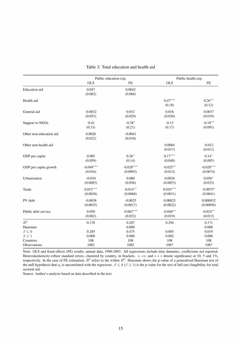
Table 3: Total education and health aid

Public education exp. Public health exp.OLS FE OLS FE

Education aid 0.047 0.0042(0.082) (0.068)

Health aid 0.47∗∗∗ 0.26∗∗

(0.18) (0.12)

General aid -0.0032 0.032 0.016 0.0037(0.053) (0.029) (0.030) (0.019)

Support to NGOs -0.41 -0.38∗ -0.13 -0.18∗∗

(0.33) (0.21) (0.17) (0.091)

Other non-education aid 0.0026 -0.0041(0.022) (0.018)

Other non-health aid 0.0084 -0.012(0.017) (0.012)

GDP per capita 0.085 0.26∗ 0.17∗∗∗ 0.14∗

(0.059) (0.14) (0.048) (0.085)

GDP per capita growth -0.049∗∗∗ -0.028∗∗∗ -0.025∗∗ -0.020∗∗∗

(0.016) (0.0093) (0.012) (0.0074)

Urbanisation -0.010 0.080 0.0026 0.056∗

(0.0083) (0.056) (0.0053) (0.033)

Trade 0.015∗∗∗ -0.014∗∗ 0.010∗∗∗ -0.0075∗

(0.0038) (0.0068) (0.0031) (0.0041)

PV debt -0.0038 -0.0025 0.00025 0.000032(0.0035) (0.0017) (0.0022) (0.00056)

Public debt service 0.050 -0.063∗∗∗ -0.040∗∗ -0.024∗∗

(0.062) (0.022) (0.019) (0.012)

R2 0.178 0.207 0.294 0.171Hausman 0.000 0.000β 6 0 0.285 0.475 0.005 0.019β > 1 0.000 0.000 0.002 0.000Countries 108 108 108 108Observations 1082 1082 1087 1087

Note: OLS and fixed effects (FE) results, annual data, 1990-2003. All regressions include time dummies, coefficients not reported.Heteroskedasticity-robust standard errors, clustered by country, in brackets. ∗, ∗∗, and ∗ ∗ ∗ denote significance at 10, 5 and 1%,respectively. In the case of FE estimation, R2 refers to the within R2. Hausman shows the p-value of a generalized Hausman test ofthe null hypothesis that ηi is uncorrelated with the regressors. β 6 0 (β > 1) is the p-value for the test of full (no) fungibility for totalsectoral aid.Source: Author’s analysis based on data described in the text.

15

The further disaggregation of sectoral aid markedly changes the results. In both sectors, the marginal effect

of SP aid in the FE model is close to 1; this result suggests that the bulk of SP aid is used in the intended

sector. Full fungibility can be rejected, but the null hypothesis of no fungibility cannot be rejected. The effect

of TC is close to zero in both sectors, and the null hypothesis of full fungibility is strongly rejected. The

hypothesis of no fungibility cannot be rejected; thus, there is no evidence that sectoral TC displaces a recipient

government’s own expenditure in either sector. The TC effect is similar in OLS, whereas the coefficients of SP

aid become larger but are also estimated less precisely. The larger SP aid coefficients in OLS may indicate that

time-invariant unobservables are positively correlated with both SP aid and sectoral public expenditures. In the

FE estimation, the coefficients are identified from the within-country variation in the data, which reduces the

problem of omitted variables in instances in which such variables do not change substantially over time.

For the FE results in Tables 3 and 4, a generalized Hausman test that allows for heteroskedasticity and

serial correlation is reported (Arellano, 1993; Wooldridge, 2002, pp. 290-291).20 The null hypothesis that

ηi is uncorrelated with the regressors is always rejected; this result suggests that FE should be preferred over

RE. Growth consistently has a negative effect, which suggests that education and health expenditures do not

immediately adjust to a higher (lower) level in the event of a positive (negative) short-term shock to GDP per

capita (Dreher, 2006, obtains a similar result for total and social expenditures in OECD countries).

As a robustness test, I obtain qualitatively similar FE results with aid variables that are constructed by

scaling up sectoral CRS disbursements to ensure that their sum matches the aggregate DAC2a disbursements

(equation (5) but applied to CRS disbursements rather than commitments). The main change is that for some

aid variables, the estimated coefficients are closer to zero and/or estimated less precisely, which is consistent

with greater measurement error in the aid data that are constructed using this short-cut method.21

Table 4 illustrates that a failure to properly address the presence of off-budget aid may yield mislead-

ing conclusions. After on- and off-budget aid are separated and their effects are assessed against appropriate

benchmarks, the FE results suggest that there is little if any fungibility. This conclusion is robust to a large

number of specification changes. I replace the PV of debt with a non-PV measure of long-term external public

and publicly guaranteed debt expressed as a percentage of GDP (from World Bank, 2006b). I also add to the

model, in turn, two different measures of the PV of debt relief constructed by Depetris Chauvin and Kraay

(2005).22 Because debt relief is often linked to higher social expenditure, one might expect it to have a larger

positive effect on public education and health expenditure than the effect achieved by a reduction in debt or

debt service that arises through means other than debt relief. If this effect is indeed larger, then we would

expect a positive effect of debt relief even after controlling for the level of debt and debt service. However.

I do not find evidence of this effect. Even without controlling for debt and debt service, I find no effect of

the PV of debt relief. I further include GDP per capita in log form rather than in thousands of dollars. I add

16

Table 4: Disaggregated education and health aid

Public education exp. Public health exp.OLS FE OLS FE

Education IP 0.091 0.12(0.25) (0.12)

Education SP 2.53∗ 1.21∗∗

(1.35) (0.55)

Education TC 0.032 -0.0070(0.10) (0.082)

Education ONM 0.14 0.021(0.21) (0.19)

Health IP 0.40 0.20(0.34) (0.21)

Health SP 1.19∗ 0.84∗∗∗

(0.60) (0.31)

Health TC -0.12 0.0067(0.35) (0.32)

Health ONM 0.74∗∗ 0.41∗

(0.36) (0.23)

General aid -0.0012 0.031 0.023 0.0055(0.051) (0.029) (0.031) (0.019)

Support to NGOs -0.56∗ -0.39∗∗ -0.15 -0.16(0.30) (0.19) (0.16) (0.11)

Other non-education aid -0.0081 -0.0055(0.022) (0.018)

Other non-health aid 0.014 -0.013(0.017) (0.011)

GDP per capita 0.084 0.29∗ 0.17∗∗∗ 0.15∗

(0.060) (0.15) (0.048) (0.085)

GDP per capita growth -0.051∗∗∗ -0.029∗∗∗ -0.028∗∗ -0.021∗∗∗

(0.015) (0.0091) (0.011) (0.0072)

Urbanisation -0.0089 0.085 0.0026 0.055∗

(0.0081) (0.055) (0.0053) (0.031)

Trade 0.016∗∗∗ -0.013∗∗ 0.011∗∗∗ -0.0071∗

(0.0039) (0.0067) (0.0032) (0.0040)

PV debt -0.0040 -0.0027∗ -0.000074 -0.000092(0.0034) (0.0016) (0.0021) (0.00059)

Public debt service 0.052 -0.065∗∗∗ -0.039∗∗ -0.022∗

(0.062) (0.021) (0.019) (0.011)

R2 0.187 0.215 0.302 0.183Hausman 0.000 0.000βSP 6 0 0.032 0.015 0.026 0.004βSP > 1 0.870 0.645 0.621 0.307βTC 6 −1 0.000 0.000 0.006 0.001βTC > 0 0.621 0.466 0.363 0.508Countries 108 108 108 108Observations 1082 1082 1087 1087

Note: OLS and fixed effects (FE) results, annual data, 1990-2003. All regressions include time dummies, coefficients not reported.Heteroskedasticity-robust standard errors, clustered by country, in brackets. ∗, ∗∗, and ∗ ∗ ∗ denote significance at 10, 5 and 1%,respectively. In the case of FE estimation, R2 refers to the within R2. Hausman shows the p-value of a generalized Hausman test ofthe null hypothesis that ηi is uncorrelated with the regressors. βSP 6 0 (βSP > 1) and βTC 6 −1 (βTC > 0) are p-values for the testof full (no) fungibility for sector programme aid and technical cooperation, respectively.Source: author’s analysis based on data described in the text.

17

(one at a time) control variables for female labor force participation or the birth rate (both from World Bank,

2006c), measures of corruption, the rule of law and bureaucratic quality from the International Country Risk

Guide (ICRG) (The Political Risk Services Group, 2008), the sum of these three ICRG variables (as a general

measure of institutional quality), and measures of democracy obtained from Polity IV (Marshall and Jaggers,

2007). Feyzioglu et al. (1998) control for the share of agriculture in GDP rather than urbanization. Therefore,

I replace urbanization with the share of agriculture in GDP (from WDI) or add the share of agriculture in GDP

alongside urbanization. Many papers also control for the size and composition of the population when explain-

ing variation in public expenditures (e.g., Baqir, 2002; Rodrik, 1998). As a result, I consider models that add

the percentage of the population under 15 and/or the percentage of the population over 65 to the model, the age

dependency ratio (dependents of the working-age population) or the log of population (all from WDI). Finally,

Feyzioglu et al. (1998) control for lagged infant mortality, whereas Devarajan et al. (2007) control for lagged

secondary and primary school enrollment in the education expenditure equation and for lagged infant mortality

in the health expenditure equation. A possible concern is that such variables may be more fruitfully viewed as

outcomes than as determinants of public education and health expenditures. Nonetheless, I include either the

current value or the once-lagged value of primary gross enrollment, secondary gross enrollment, infant mortal-

ity or under-five mortality (mortality data from WDI and enrollment data from Edstats). In all cases, the results

are qualitatively unchanged. The only exception is that when the ICRG measures are added, the coefficient

of health TC decreases to approximately -0.25, and I can reject the null hypothesis of no fungibility, implying

partial (but low) fungibility of health TC.23

Influential observations

Especially given the limited variation in education and health SP aid and, to a lesser extent, TC, one concern

may be that the effects of these variables are driven by a small number of observations. Although the inclusion

of additional control variables generally does not change the conclusions, the point estimates on the variables

of interest shift by a relatively large amount in several instances, especially when the inclusion of an additional

variable leads to a large decrease in sample size. Such a shift always results from a change in the sample com-

position and not because the additional control variable eliminates some of the explanatory power of sectoral

SP aid or TC.24

As a first attempt to evaluate the sensitivity of the results to outliers, I re-estimate equation (11) in log-linear

form. Taking the natural logarithm of all variables compresses the upper tail and is thus likely to reduce the

influence of observations with larger values of education and health SP aid or TC on the estimated regression

line.25 Table 5 displays the marginal effects for SP aid and TC calculated at the sample means (the full results

are available upon request). The results are similar to those obtained in the linear model. In both sectors, the

18

effect of TC is close to zero, and the effect of SP aid on public expenditure is close to 1. Full fungibility is

rejected across the board, but the null hypothesis of no fungibility cannot be rejected in any of the cases.

Table 5: Disaggregated education and health aid, marginal effects of the log-linear model

Public education exp. Public health exp.

βSP 1.342 1.092βSP 6 0 0.005 0.006βSP > 1 0.750 0.585βTC 0.0522 0.0602βTC 6 −1 0.000 0.000βTC > 0 0.632 0.591

Note: βSP and βTC are marginal effects, calculated at the sample means, based on the fixed effects estimation of equation (11) in log-linear form. Annual data, 1990-2003. All regressions include time dummies and the standard set of control variables (coefficients notreported) and are estimated with heteroskedasticity-robust standard errors, clustered by country. βSP 6 0 (βSP > 1) and βTC 6 −1(βTC > 0) are p-values for the test of full (no) fungibility for sector program aid and technical cooperation, respectively.Source: Author’s analysis based on data described in the text.

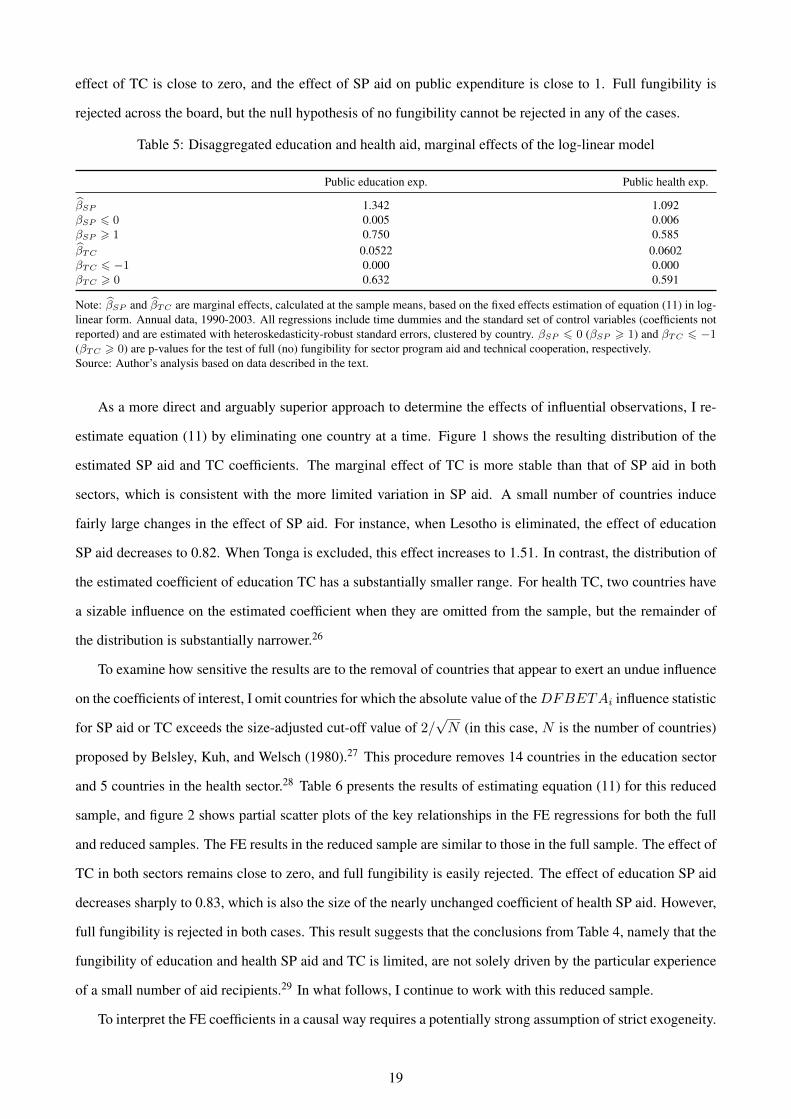
As a more direct and arguably superior approach to determine the effects of influential observations, I re-

estimate equation (11) by eliminating one country at a time. Figure 1 shows the resulting distribution of the

estimated SP aid and TC coefficients. The marginal effect of TC is more stable than that of SP aid in both

sectors, which is consistent with the more limited variation in SP aid. A small number of countries induce

fairly large changes in the effect of SP aid. For instance, when Lesotho is eliminated, the effect of education

SP aid decreases to 0.82. When Tonga is excluded, this effect increases to 1.51. In contrast, the distribution of

the estimated coefficient of education TC has a substantially smaller range. For health TC, two countries have

a sizable influence on the estimated coefficient when they are omitted from the sample, but the remainder of

the distribution is substantially narrower.26

To examine how sensitive the results are to the removal of countries that appear to exert an undue influence

on the coefficients of interest, I omit countries for which the absolute value of theDFBETAi influence statistic

for SP aid or TC exceeds the size-adjusted cut-off value of 2/√N (in this case, N is the number of countries)

proposed by Belsley, Kuh, and Welsch (1980).27 This procedure removes 14 countries in the education sector

and 5 countries in the health sector.28 Table 6 presents the results of estimating equation (11) for this reduced

sample, and figure 2 shows partial scatter plots of the key relationships in the FE regressions for both the full

and reduced samples. The FE results in the reduced sample are similar to those in the full sample. The effect of

TC in both sectors remains close to zero, and full fungibility is easily rejected. The effect of education SP aid

decreases sharply to 0.83, which is also the size of the nearly unchanged coefficient of health SP aid. However,

full fungibility is rejected in both cases. This result suggests that the conclusions from Table 4, namely that the

fungibility of education and health SP aid and TC is limited, are not solely driven by the particular experience

of a small number of aid recipients.29 In what follows, I continue to work with this reduced sample.

To interpret the FE coefficients in a causal way requires a potentially strong assumption of strict exogeneity.

19

Table 6: Disaggregated education and health aid, reduced sample

Public education exp. Public health exp.FE FD FE FD

Education IP 0.22 0.34∗∗∗

(0.15) (0.12)

Education SP 0.83∗∗ -0.34(0.34) (0.55)

Education TC 0.024 -0.070(0.059) (0.046)

Education ONM -0.25 -0.044(0.24) (0.11)

Health IP 0.17 -0.19∗

(0.19) (0.11)

Health SP 0.83∗∗ -0.19(0.36) (0.24)

Health TC -0.15 -0.040(0.20) (0.10)

Health ONM 0.31∗ 0.095(0.17) (0.12)

General aid 0.027 0.00092 0.0082 -0.0074(0.020) (0.015) (0.018) (0.011)

Support to NGOs -0.48 -0.17 -0.055 -0.025(0.31) (0.23) (0.14) (0.073)

Other non-education aid 0.00046 0.0049(0.016) (0.010)

Other non-health aid -0.019∗ 0.0039(0.011) (0.0047)

GDP per capita 0.22∗ -0.058 0.093 0.13∗∗

(0.12) (0.088) (0.071) (0.063)

GDP per capita growth -0.019∗∗∗ -0.0079∗∗ -0.015∗∗∗ -0.011∗∗∗

(0.0045) (0.0031) (0.0043) (0.0031)

Urbanisation 0.039 0.0033 0.019 0.017(0.045) (0.064) (0.025) (0.026)

Trade -0.0035 -0.0025 -0.0013 0.00046(0.0041) (0.0037) (0.0023) (0.0021)

PV debt -0.0055∗∗ -0.0038 -0.00026 -0.00017(0.0025) (0.0038) (0.00056) (0.00072)

Public debt service -0.059∗∗∗ -0.024∗ -0.019 -0.0031(0.019) (0.012) (0.012) (0.0057)

R2 0.183 0.062 0.135 0.051Hausman 0.000 0.000βSP 6 0 0.008 0.731 0.012 0.781βSP > 1 0.307 0.008 0.313 0.000βTC 6 −1 0.000 0.000 0.000 0.000βTC > 0 0.658 0.066 0.239 0.347Countries 94 94 103 102Observations 921 819 1024 912

Note: fixed effects (FE) and first-differenced OLS (FD) results, annual data, 1990-2003, reduced sample. All regressions include timedummies, coefficients not reported. Heteroskedasticity-robust standard errors, clustered by country, in brackets. ∗, ∗∗, and ∗ ∗ ∗ denotesignificance at 10, 5 and 1%, respectively. In the case of FE estimation, R2 refers to the within R2. Hausman shows the p-value ofa generalized Hausman test of the null hypothesis that ηi is uncorrelated with the regressors. βSP 6 0 (βSP > 1) and βTC 6 −1(βTC > 0) are p-values for the test of full (no) fungibility for sector programme aid and technical cooperation, respectively.Source: Author’s analysis based on data described in the text.

20

Figure 1: Distribution of coefficients when dropping one country at a time

(a) Education SP aid

020

4060

80F

requ

ency

.8 1 1.2 1.4 1.6Education SP aid

(b) Education TC

020

4060

80F

requ

ency

−.04 −.02 0 .02 .04Education TC

(c) Health SP aid

020

4060

80F

requ

ency

.6 .7 .8 .9 1 1.1Health SP aid

(d) Health TC

020

4060

80F

requ

ency

−.3 −.2 −.1 0 .1Health TC

Source: Author’s analysis based on data described in the text.

This assumption would be violated if, for instance, the allocation of education (health) SP aid and TC were

partially determined on the basis of past or current values of public education (health) expenditure. In fact,

Table 6 contains some evidence indicating that strict exogeneity for SP aid is unlikely to hold. If a first-

differenced version of equation (11) is estimated with OLS (columns 2 and 4, labeled FD), then the effect of

SP aid differs markedly from its FE estimate and even becomes negative. This stark difference between the FE

and FD estimates of the SP aid coefficients suggests a violation of the strict exogeneity assumption because

such a violation causes both FE and FD to be inconsistent and to have different probability limits (Wooldridge,

2002, pp. 284-285). However, the effect of TC is similar in the first-differenced model. There is some evidence

of a negative effect of TC, especially in the education sector, in which the hypothesis of no fungibility can be

rejected at a 10% significance level, but any displacement of sectoral public expenditure is minimal. Hence,

the conclusion that the fungibility of TC is limited is confirmed in the FD model. A second indication that the

FE model may be misspecified emerges from a serial correlation test of the idiosyncratic errors.30 For both

sectors, I reject the null hypothesis of no serial correlation at a significance level of less than 1%. Although

clustering standard errors on the recipient country should ensure that inferences are valid, the presence of a

serial correlation in εit may indicate that the model is dynamically misspecified, which would again render the

21

Figure 2: Partial scatter plots

(a) Education SP aid

−4

−2

02

4P

ublic

edu

catio

n ex

pend

iture

−.2 0 .2 .4 .6Education SP aid

(b) Education TC

−4

−2

02

4P

ublic

edu

catio

n ex

pend

iture

−2 −1 0 1 2 3Education TC

(c) Health SP aid

−1

01

23

Pub

lic h

ealth

exp

endi

ture

−.4 −.2 0 .2 .4Health SP aid

(d) Health TC

−1

01

23

Pub

lic h

ealth

exp

endi

ture

−.5 0 .5 1Health TC

Note: Partial scatter plots in the full (solid line) and reduced (dotted line) samples correspond to the FE resultsin Tables 4 and 6, respectively. + denotes observations that are excluded from the reduced sample.Source: Author’s analysis based on data described in the text.

FE estimates inconsistent.

Therefore, I also examine the results that are obtained when the strict exogeneity assumption is relaxed by

employing a system GMM estimator (Arellano and Bover, 1995; Blundell and Bond, 1998). This estimator

further enables the consistent estimation of a more general model that includes a lagged dependent variable

(which removes the serial correlation in εit):31

SSPit = αSSPi,t−1 + βIPSAIDIPit + βSPSAIDSPit + βTCSAIDTCit

+ βONMSAIDONMit + γAit + δXit + λt + ηi + εit. (12)

Equation (12) is estimated using a two-step system GMM estimator applying Windmeijer’s (2005) correc-

tion for the downward bias in the two-step standard errors. All education (health) aid prefix code variables,

support to NGOs, and trade are treated as endogenous, whereas all other variables are treated as predetermined.

Time dummies are treated as strictly exogenous and are thus added to the instrument matrix without transfor-

mation. I reduce the risk of overfitting by restricting the maximum number of lags of the level variables that

22

are used as instruments for the differenced equation32 and by collapsing the instrument matrix, which creates

an instrument for each variable and lag distance rather than for each variable, time period, and lag distance

(Roodman, 2009a,b). To conserve space, I do not report the system GMM results and discuss them only briefly

(the full results and a more detailed discussion are available in the working paper version of this article).

The short-term effect of SP aid in both sectors is near zero but is volatile across the different instrument

configurations and is estimated imprecisely. As a result, neither the null hypothesis of full fungibility nor the

null hypothesis of no fungibility can typically be rejected at conventional significance levels. This volatility

and imprecision carry over to the estimate of the long-term effect of education SP aid, βLRSP = βSP /(1 − α).

This imprecision likely results from the lack of variation in SP aid. The effect of education TC is close to zero,

and the null hypothesis of full fungibility is always strongly rejected. No fungibility cannot be rejected, and the

point estimate suggests, at most, only minor displacement of public education expenditures by education TC

in the short term. Given the persistence in public education expenditures, the estimate of the long-term effect

of education TC is more negative (with -0.3 as the lowest estimate), but even in the long term, full fungibility

is rejected and no fungibility is not rejected. In the health sector, full fungibility of TC in the short term is

also rejected across the board. In fact, health TC is found to have a positive effect, although the estimate is

never significantly different from zero. The average estimated LR effect is approximately 2.6 but has a large

standard error. Nonetheless, in all cases except when only a single lag of the variables is used to instrument the

differenced equation, full fungibility in the long term can still be rejected. Similar long-term effects are found

when a lag of TC aid is added as an explanatory variable in equation (12).

An alternative assessment

Finally, it is worthwhile to consider an alternative approach that allows for a broader assessment of the degree

of fungibility of education and health aid while allowing for some uncertainty in the measurement of on- and

off-budget aid. Beginning with (3), the estimated coefficient of health aid in (2) can be written as follows:33

β = βONw + βOFF (1− w) , (13)

with weight w,

w =1 + ρ

√δ

1 + δ + 2ρ√δ, (14)

and with ρ =σON,OFFσONσOFF

as the correlation between on- and off-budget health aid and δ =σ2OFF

σ2ON

as the relative

variance of off- versus on-budget health aid. If we impose that on- and off-budget health aid have the same

degree of fungibility (βOFF = βON − 1), then we can rearrange equation (13) to express βON as a function of

23

β:

βON = β + 1− 1 + ρ√δ

1 + δ + 2ρ√δ. (15)

This equation demonstrates how, for given values of ρ and δ, our naive estimate of β can be used to generate

an estimate (βON ) that can be used to determine the degree of fungibility: a value of βON that is close to 1

indicates that there is little or no fungibility, whereas a value that is closer to 0 suggests a greater degree of

fungibility.34 Table 7 performs this computation for total aid and for each of the 4 aid types in both sectors,

beginning with the FE coefficients that are estimated in Tables 3 and 4, respectively. For each variable, the

entries in the table calculate βON for different values of the relative variance of off- versus on-budget aid in the

aid type considered (δ, ranging from 1/4 to 4) and the correlation between its on- and off-budget components

(ρ, ranging from -1 to 1). A bold (underlined) entry indicates that the null hypothesis of full (no) fungibility

can be rejected at a 5% significance level.

After partialling out the fixed effects and the control variables, the correlations between the four different

aid types (IP, SP, TC and ONM) are a useful indication of the most plausible values of ρ for total education and

health aid. In both sectors, these correlations are close to zero. The most negative correlation is between health

SP aid and TC (-0.15), and the most positive correlation is between education TC and ONM (0.14). Hence, ρ

is not expected to be far from 0. Meanwhile, it is very likely that most of the variation in total education and

health aid is driven by off-budget aid (implying δ > 1). Technical assistance, which I have argued is almost

entirely off-budget, dominates the variation in health and, especially, education aid (see Table 1), while there is

some evidence to suggest that the other non-program components are also not well captured in the budgets of

recipient governments (see section III). Hence, the entries in the bottom four rows of Tables 7a and 7b are the

most plausible. Especially in the health sector, these entries indicate a low degree of fungibility. For health aid,

the null hypothesis of no fungibility is never rejected for δ > 3/2; even for a δ value as low as 1/2, a fairly low

degree of fungibility is found for most values of ρ.

With regard to the aid types, even under the assumption that SP aid is completely on-budget, its estimated

FE coefficient in Table 4 for both sectors implies low fungibility. Hence, it is not surprising that this conclusion

is confirmed in Tables 7e and 7f.35 Tables 7g and 7h relax the assumption that TC is completely off-budget.

In almost all cases, the null hypothesis of full fungibility can still be rejected, and most entries suggest limited

fungibility. For health TC, the null hypothesis of no fungibility is never rejected. The vast majority of entries

in Table 7j indicate a low degree of fungibility of health ONM aid, with few rejections of the null hypothesis

of no fungibility. The degree of fungibility is higher for education ONM aid and is more difficult to assess.

Both null hypotheses are typically rejected; thus, the results suggest partial fungibility, but the exact degree of

fungibility depends on the relative variation of off-budget versus on-budget aid, which is difficult to determine.

The discussion in section III suggests that aid projects (IP) are frequently not captured in the budgets of recipient

24

Table 7: Fungibility of education and health aid

(a) Education aid

ρ-1 -3/4 -1/2 0 1/2 3/4 1

δ

1/4 -1.00 -0.25 0.00 0.20 0.29 0.32 0.341/2 -2.41 -0.06 0.19 0.34 0.39 0.41 0.423/4 -6.46 0.23 0.36 0.43 0.46 0.46 0.471 . 0.50 0.50 0.50 0.50 0.50 0.503/2 5.45 0.88 0.70 0.60 0.57 0.56 0.552 3.42 1.07 0.82 0.67 0.62 0.60 0.594 2.00 1.25 1.00 0.80 0.72 0.69 0.67

(b) Health aid

ρ-1 -3/4 -1/2 0 1/2 3/4 1

δ

1/4 -0.74 0.01 0.26 0.46 0.54 0.57 0.591/2 -2.16 0.19 0.44 0.59 0.65 0.66 0.673/4 -6.21 0.48 0.62 0.69 0.71 0.72 0.721 . 0.76 0.76 0.76 0.76 0.76 0.763/2 5.71 1.14 0.96 0.86 0.83 0.82 0.812 3.67 1.33 1.07 0.93 0.87 0.86 0.844 2.26 1.51 1.26 1.06 0.97 0.95 0.93

(c) Education IP

ρ-1 -3/4 -1/2 0 1/2 3/4 1

δ

1/4 -0.88 -0.13 0.12 0.32 0.41 0.44 0.461/2 -2.29 0.05 0.31 0.46 0.51 0.53 0.543/4 -6.34 0.35 0.48 0.55 0.57 0.58 0.591 . 0.62 0.62 0.62 0.62 0.62 0.623/2 5.57 1.00 0.82 0.72 0.69 0.68 0.672 3.54 1.19 0.94 0.79 0.74 0.72 0.714 2.12 1.37 1.12 0.92 0.84 0.81 0.79

(d) Health IP

ρ-1 -3/4 -1/2 0 1/2 3/4 1

δ

1/4 -0.80 -0.05 0.20 0.40 0.49 0.51 0.531/2 -2.21 0.13 0.38 0.53 0.59 0.60 0.613/4 -6.26 0.42 0.56 0.63 0.65 0.66 0.661 . 0.70 0.70 0.70 0.70 0.70 0.703/2 5.65 1.08 0.90 0.80 0.77 0.76 0.752 3.61 1.27 1.02 0.87 0.81 0.80 0.794 2.20 1.45 1.20 1.00 0.91 0.89 0.87

(e) Education SP aid

ρ-1 -3/4 -1/2 0 1/2 3/4 1

δ

1/4 0.21 0.96 1.21 1.41 1.49 1.52 1.541/2 -1.21 1.14 1.39 1.54 1.59 1.61 1.623/4 -5.26 1.43 1.56 1.63 1.66 1.66 1.671 . 1.71 1.71 1.71 1.71 1.71 1.71

(f) Health SP aid

ρ-1 -3/4 -1/2 0 1/2 3/4 1

δ

1/4 -0.16 0.59 0.84 1.04 1.13 1.16 1.181/2 -1.57 0.78 1.03 1.18 1.23 1.25 1.263/4 -5.62 1.07 1.20 1.27 1.30 1.30 1.311 . 1.34 1.34 1.34 1.34 1.34 1.34

(g) Education TC

ρ-1 -3/4 -1/2 0 1/2 3/4 1

δ

1 . 0.49 0.49 0.49 0.49 0.49 0.493/2 5.44 0.87 0.69 0.59 0.56 0.55 0.542 3.41 1.06 0.81 0.66 0.61 0.59 0.584 1.99 1.24 0.99 0.79 0.71 0.68 0.66

(h) Health TC

ρ-1 -3/4 -1/2 0 1/2 3/4 1

δ

1 . 0.51 0.51 0.51 0.51 0.51 0.513/2 5.46 0.88 0.70 0.61 0.57 0.56 0.562 3.42 1.08 0.82 0.67 0.62 0.60 0.594 2.01 1.26 1.01 0.81 0.72 0.69 0.67

(i) Education ONM aid

ρ-1 -3/4 -1/2 0 1/2 3/4 1

δ

1/4 -0.98 -0.23 0.02 0.22 0.31 0.33 0.351/2 -2.39 -0.05 0.21 0.35 0.41 0.42 0.433/4 -6.44 0.24 0.38 0.45 0.47 0.48 0.481 . 0.52 0.52 0.52 0.52 0.52 0.523/2 5.47 0.90 0.72 0.62 0.59 0.58 0.572 3.43 1.09 0.84 0.69 0.63 0.62 0.614 2.02 1.27 1.02 0.82 0.73 0.71 0.69

(j) Health ONM aid

ρ-1 -3/4 -1/2 0 1/2 3/4 1

δ

1/4 -0.59 0.16 0.41 0.61 0.70 0.73 0.751/2 -2.00 0.35 0.60 0.75 0.80 0.82 0.833/4 -6.05 0.64 0.77 0.84 0.87 0.87 0.881 . 0.91 0.91 0.91 0.91 0.91 0.913/2 5.86 1.29 1.11 1.01 0.98 0.97 0.962 3.83 1.48 1.23 1.08 1.03 1.01 1.004 2.41 1.66 1.41 1.21 1.13 1.10 1.08

Note: The entries in this table are the values of βON computed according to equation (15) for different aidvariables, starting from the FE coefficients estimated in Tables 3 and 4. ρ is the correlation between the on-and off-budget components of the aid variable, δ the relative variance of the off- versus on-budget componentof the aid variable. Bold (underlined) entries indicate that the null of full (no) fungibility is rejected at a 5%significance level.Source: Author’s analysis based on data described in the text.

25

governments. Even when the relative variance of off- versus on-budget IP aid is 1 or slightly below 1, the entries

in Tables 7c and 7d again indicate fairly low degrees of fungibility, especially in the health sector. Hence, unless

ρ is very negative, we would only be comfortable concluding that IP is mostly fungible if we believe that the

variance in off-budget IP is substantially lower than the variance in on-budget IP.

V Conclusion

This paper presents new empirical evidence to provide insight into the difficult issue of foreign aid fungibility.

I construct data on earmarked education and health aid disbursements that also distinguish between on- and off-

budget components of aid. Sector program aid measures on-budget aid, whereas technical cooperation proxies

for off-budget aid. I illustrate how a failure to adequately address the presence of off-budget aid may have

biased previous estimates of foreign aid fungibility.

Overall, I find little evidence that aid is fully or even largely fungible; rather, most point estimates suggest

limited fungibility. In both sectors, technical cooperation leads to, at most, a small displacement of a recipient’s

own public spending. This effect is estimated relatively tightly, especially in the education sector. Thus, the

results suggest a genuine effect rather than merely noise in the data. The effect of technical cooperation is

robust across a range of models, whereas the effect of sector program aid is more volatile. In a static panel data

model, fixed effects results suggest an approximately one-to-one correlation between sector program aid and

public sectoral expenditure, which is robust to a large number of specification changes. However, when system

GMM is used to estimate a dynamic model, the effect of sector program aid is imprecisely estimated. Thus, no

firm conclusions can be drawn with respect to the fungibility of sector program aid.

Therefore, the result of limited fungibility for education and health aid specifically pertains to technical

cooperation. Because technical cooperation is the dominant modality in both sectors, however, it plays a large

role in determining the overall degree of fungibility of earmarked education and health aid. The extent to

which investment projects and other aid are on- or off-budget is more uncertain, making it more difficult to

determine the degree to which these projects are fungible. However, the analysis in section IV suggests that

unless we believe that the variance of the on-budget components of investment projects and other aid dominates

the variance of their off-budget components, both types of aid are far from fully fungible.

The lack of fungibility may be a consequence of effective donor conditionality. If donors are able to

monitor the spending of recipient governments, then they may be able to credibly enforce the condition that

aid adds to the resources that are spent in the targeted sector. An additional reason for the low degree of

fungibility primarily applies to technical cooperation and is less applicable to other aid types. This explanation

is the observation made by Gramlich (1977) that heterogeneity in government expenditures may contribute

to reduced fungibility. To the extent that governments in developing countries spend few resources on the

26

type of goods and services that are provided by technical cooperation, it becomes impossible to significantly

reduce this class of expenditure because these expenditures rapidly approach the lower bound of zero. If

the substitutability between different types of expenditures in a recipient government’s utility function is also

limited, then low fungibility for technical cooperation may ensue. Finally, a lack of information on the part of a

recipient government, which is particularly relevant for off-budget aid, may also reduce the degree of fungibility

that is observed in practice.

From the donor perspective, the results in this paper suggest that the costly effort associated with earmarking

(e.g., monitoring costs) may not be futile. From the perspective of the population in a recipient country, the

limited fungibility of education and health aid can be perceived as a positive result if we believe that better

education and health have positive consequences for human welfare. However, this positive interpretation

persists only if the aid in these sectors effectively produces valuable outcomes. Moreover, if the low fungibility

of off-budget aid arises because a recipient government is not fully aware of this aid, then any positive effects of

non-fungible off-budget aid must be balanced against the possible deleterious effects on government capacity

and ownership that are incurred when channeling funds outside of a budget. In general, not a great deal is

known about the normative consequences of fungibility (for papers that look at this issue, see McGillivray and

Morrissey, 2000; Pettersson, 2007b,a; Wagstaff, 2011), and this constitutes an important area for future study.

Notes

1Even if every dollar of health aid is spent in the health sector, health aid may still be fungible if the recipient government reduces

health expenditures from its own resources. I discuss this situation in greater detail below with respect to the fungibility of off-budget

aid.

2Implicitly, this test assumes that off-budget aid resources cannot be directly diverted to other purposes because this direct diversion

of off-budget aid would not reduce HSP . For example, if medicines are supplied by donors as off-budget health aid, then this

assumption implies that a recipient government cannot sell these medicines and spend the proceeds in another sector. As a result, the

only way for a recipient government to render off-budget health aid fungible is to reduce its own health expenditure, which is tested in

equation (1). The exclusion of off-budget aid from budgetary records reflects a lack of exclusive control of the government over these

resources; thus, according to its nature, most off-budget aid should fall into this category of aid that cannot directly be diverted to other

sectors. Even if this categorization does not apply to all types of off-budget aid, in the empirical application below, I focus on a specific

type of off-budget aid, technical cooperation, for which this assumption is plausible.

3For simplicity, the exposition focuses on a cross-sectional case without control variables. Later in the paper, I will primarily

examine panel data models that include control variables and that use a fixed effects estimator. In these models, the variables in

equation (1) and (2) can be understood as the residuals of the variables after the fixed effects and control variables have been partialled

out. In that case, in (3), σ2ON , σ2

OFF , σ2 and σON,OFF refer to the variances and covariance of the partialled-out versions of the

relevant variables.

4I am grateful to an anonymous referee for suggesting this framework to discuss the bias that may be caused by off-budget aid.

5Other studies report similarly large shares of off-budget aid out of total aid but do not allow us to assess the extent of variation

27

in off-budget aid over time. In Fiji and Vanuatu, 70% of all aid is off-budget aid (Feeny, 2007). In Malawi, approximately 40% is

off-budget aid (Fagernas and Schurich, 2004), and in Liberia, approximately 75% is off-budget aid (Republic of Liberia Ministry of

Finance, 2009).

6For example, suppose that in the absence of any health aid, a recipient government spends 100 million dollars in the health sector.

If a donor provides 200 million dollars of off-budget health aid, then full fungibility would entail that the recipient government reduces

its own health expenditures at an approximately one-to-one rate (i.e., the recipient government reduces its health expenditure by 200

million dollars). However, the government cannot implement such a reduction because health expenditure would need to decrease

below zero. The most that this government can do is to reduce its health expenditure by 100 million dollars; in this situation, health aid

is only partially fungible.

7Many of the papers in this body of literature disaggregate aid into grants and loans, multilateral and bilateral aid, or by aid modality,

but not by sector.

8The studies that are referenced in this paragraph estimate the degree of fungibility using panel data for either a large (Feyzioglu

et al., 1998; Devarajan et al., 2007) or small (Heller, 1975; Feeny, 2007) number of countries, or they report country-specific estimates

of fungibility (all other studies referenced in this paragraph).

9I describe the OECD’s aid databases as they were when I began to construct the sectoral aid data (December 2006). Since then, the

CRS and DAC Directives have been updated, and the databases have undergone minor changes (see OECD, 2007a,b).

10RY denotes recipient-year, agg denotes aggregate aid, and comm denotes commitments. No superscript is used for disbursements.

11The data in DAC5 are a mix of disbursements and commitments. To account for this, I scale the DAC5 data to ensure that the sum

of the sectoral aid variables matches the aggregate disbursements from DAC2a for every donor-year.

12Since the construction of the data for this paper, two new disaggregated aid datasets have become available. Ravishankar, Gubbins,

Cooley, Leach-Kemon, Michaud, Jamison, and Murray (2009) construct data on health aid by estimating disbursements on the basis

of the less incomplete CRS commitments and by adding data from separate reports for a number of NGOs and multilateral and private

donors. These data are used by Lu et al. (2010) to estimate the fungibility of health aid. One disadvantage is that a large portion

of the data cannot be allocated by recipient country. Lu et al. (2010, p. 1379) state that only 21% of all health aid in 1995 can be

traced to recipient countries, and 30% of this aid can be traced to recipient countries in 2006. In addition, it is not immediately clear

how one would further divide health aid into on- and off-budget components in these data. A second recent dataset, AidData (http:

//www.aiddata.org), attempts to construct a more complete disaggregation of aggregate aid into all of its constituent parts according to

a number of dimensions but focuses almost exclusively on commitments.

13Current US$ GDP from World Bank (2006c) is used to express sectoral aid disbursements as a percentage of the GDP.

14These data are not publicly available, although they have been used in a variety of publications (e.g., Gupta, Clements, and

Tiongson, 1998; Baqir, 2002). I am grateful to Gerd Schwartz for sharing these data and to Ali Abbas for assistance in obtaining them.

15For Fiji, the observation in 1998 for both sectors is approximately ten times smaller than that in the surrounding years, most

likely due to a typographical error. For instance, public education expenditures account for 0.572% of the GDP in 1998, whereas these

expenditures range from 5.19% to 6.37% of the GDP in all other years from 1993 to 2002. Hence, I change this value to 5.72. Similarly,

I adjust the public health expenditure value for 1998 from 0.253% to 2.53% of GDP.

16Only for Paris Club concessional debt reorganizations is the net present value reduction in debt achieved by the current rescheduling

recorded (OECD, 2000b, p. 17).

17I am grateful to Ibrahim Levent for sending me the updated data (received December 2006) and the Dikhanov paper.

18Mokoro (2008) expressly warns against the assumption that aid projects are always off-budget (p. 7) but suggests that the degree

to which these projects are captured in budgets is low. (See, e.g., p. 23: “levels of aid on budget are strongly driven by budget support

aid (which, by definition, is on budget). In many cases, off budget proportions for other aid modalities still remain very high” and p.

28

52: “however, budget support has limits, and project aid has been growing. The problems associated with poorly integrated project aid

still loom large. The bigger challenge, therefore, is to bring project aid on budget.”) In section IV, I discuss how we can gain insight

into the degree of fungibility of IP and ONM aid despite the greater uncertainty regarding the extent to which these types of aid are on-

or off-budget.

19As explained in Devarajan et al. (2007), unconditional resourcesR (or their component parts, domestic revenue and net borrowing)

should be excluded from the estimated equation to ensure that the full effect of earmarked aid on sectoral spending is captured. For

instance, if sectoral aid reduces tax revenue but the latter is held fixed, then the effect of aid on spending may be overestimated. This two-

step procedure entails the inclusion of the residual from a regression of R on the right-side variables in equation (11) as an explanatory

variable in the model. Because this residual is, by construction, orthogonal to the other right-side variables, its inclusion does not alter

the sectoral aid coefficients, which capture the full effect of earmarked aid. However, its inclusion facilitates the estimation of ∂SSPit∂Rit

.

20This test is performed in Stata using the xtoverid command (Schaffer and Stillman, 2006).

21For instance, the coefficient on education SP aid is almost halved, to 0.64, and full fungibility is therefore rejected less strongly.

The coefficient on health aid is reduced to 0.07, whereas in the disaggregated model, the coefficients on health IP and health ONM

are much closer to zero. In both sectors, the coefficient on support to NGOs is estimated less precisely and/or substantially reduced in

magnitude. The only exception is that the coefficient on health SP aid nearly doubles with the short-cut method (from 0.84 to 1.61), but

its standard error rises commensurably.

22I am grateful to Nicolas Depetris Chauvin for sharing these data.

23In addition, no clear evidence is found to suggest that the degree of fungibility depends on the quality of institutions.

24The most extreme deviation occurs when the birth rate is added: the sample size in the health model decreases to 612, and the

effect of health SP aid in the FE model rises to 1.34.

25To address zero values in the public expenditure, aid and debt variables, I add 1 before taking the log. Because GDP per capita

growth can be negative, I include this variable without taking its log.

26Without Eritrea, the estimated effect of education TC becomes -0.33. Without Guinea-Bissau, the effect is 0.16.

27Using SP aid as an example, I calculate DFBETAi as DFBETAiSP = (βiSP − βSP )/(SEβiSP

), where βSP is the estimated

coefficient in the full sample, βiSP is the estimate when country i is eliminated and SEβiSP

is the estimated standard error of the

coefficient in the model without country i (see, e.g., Bollen and Jackman, 1990).

28These countries are Burkina Faso, Cote d’Ivoire, Eritrea, Guinea-Bissau, Guyana, Lesotho, Mozambique, Nicaragua, Papua New

Guinea, Samoa, Seychelles, Sierra Leone, Tajikistan and Tonga for education and Eritrea, Guinea-Bissau, Sierra Leone, Tajikistan, and

Zambia for health.

29The elimination of outliers that are identified by either the method proposed by Hadi (1992, 1994) (hadimvo in Stata) or the

method proposed by Billor, Hadi, and Velleman (2000) (bacon in Stata, see Weber, 2010) yields similar results. I follow Roodman

(2007) in applying these methods to the partialled-out versions of public sectoral expenditure and sectoral SP aid and TC (i.e., the

residuals that are obtained from the FE regressions of these variables on the other variables).

30Under the null hypothesis of no serial correlation, the residuals in the first-differenced model should have an autocorrelation of

-0.5. Thus, a Wald test of this hypothesis can be performed to test for the presence of serial correlation in εit (Wooldridge, 2002, p.

283; Drukker, 2003). I conduct this test in Stata using the xtserial command.

31Briefly, the GMM estimator differences equation (12) to remove the fixed effect and uses suitably lagged levels of the dependent

variable and the right-side variables as instruments for the differenced equation. In addition, the system GMM estimator utilizes the

equation in levels, using suitably lagged differences as instruments.

32I examine a number of different instrument configurations, from the use of a single lag of each variable to instrument the differenced

equation to the use of four lags of each variable.

29

33As in section I, I focus on the fungibility of health aid for the sake of concreteness.

34As noted previously, in a model that includes control variables and that is estimated using a FE estimator, ρ refers to the correlation

between the partialled-out versions of off- and on-budget aid, and δ refers to the relative variance of the partialled-out versions of off-

versus on-budget aid.

35For SP aid, I consider only δ 6 1, and for TC, I consider only δ > 1.

30

References

Adam, Christopher S., Per-Ake Andersson, Arne Bigsten, Paul Collier, and Steve O’Connell. 1994. “Evaluation

of Swedish development co-operation with Zambia.” Stockholm: Ministry of Foreign Affairs, Secretariat for

analysis of Swedish development assistance, Report 6.

Arellano, Manuel. 1987. “Computing robust standard errors for within-groups estimators.” Oxford Bulletin of

Economics and Statistics 49(4): 431–434.

Arellano, Manuel. 1993. “On the testing of correlated effects with panel data.” Journal of Econometrics 59(1-2):

87–97.

Arellano, Manuel and Olympia Bover. 1995. “Another look at the instrumental variable estimation of error-

components models.” Journal of Econometrics 68(1): 29–51.

Baqir, Reza. 2002. “Social sector spending in a panel of countries.” Washington, D.C.: International Monetary

Fund, Working Paper 02/35.

Baser, Heather and Peter Morgan. 2001. “The pooling of technical assistance: an overview based on field

research experience in six African countries.” A study for the Directorate-General for Development Cooper-

ation (DGIS), Ministry of Foreign Affairs of the Netherlands.

Belsley, David A., Edwin Kuh, and Roy E. Welsch. 1980. Regression diagnostics: identifying influential data

and sources of collinearity. New York: John Wiley & Sons.

Bertrand, Marianne, Esther Duflo, and Sendhil Mullainathan. 2004. “How much should we trust differences-

in-differences estimates.” Quarterly Journal of Economics 119(1): 249–275.

Billor, Nedret, Ali S. Hadi, and Paul F. Velleman. 2000. “BACON: blocked adaptive computationally efficient

outlier nominators.” Computational Statistics & Data Analysis 34: 279–298.

Blundell, Richard and Stephen Bond. 1998. “Initial conditions and moment restrictions in dynamic panel data

models.” Journal of Econometrics 87(1): 115–143.

Bollen, Kenneth A. and Robert W. Jackman. 1990. “Regression diagnostics: an expository treatment of outliers

and influential cases.” In John Fox and J. Scott Long, eds., Modern methods of data analysis, London: Sage.

Chatterjee, Santanu, Paola Giuliano, and Ilker Kaya. 2007. “Where has all the money gone? Foreign aid and

the quest for growth.” Bonn: Institute for the Study of Labor (IZA), Discussion Paper No. 2858.

Depetris Chauvin, Nicolas and Aart Kraay. 2005. “What has 100 billion dollars worth of debt relief done for

low-income countries.” Washington, D.C.: World Bank, mimeo.

31

Devarajan, Shantayanan, Andrew Sunil Rajkumar, and Vinaya Swaroop. 2007. “What does aid to Africa fi-

nance.” In Sajal Lahiri, ed., Theory and practice of foreign aid, Amsterdam: Elsevier.

Dikhanov, Yuri. 2004. “Historical PV of debt in developing countries, 1980-2002.” Washington, D.C.: World

Bank, mimeo.

Dreher, Axel. 2006. “The influence of globalization on taxes and social policy: an empirical analysis for OECD

countries.” European Journal of Political Economy 22(1): 179–201.

Drukker, David M.. 2003. “Testing for serial correlation in linear panel-data models.” Stata Journal 3(2): 168–

177.

Fagernas, Sonja and John Roberts. 2004a. “The fiscal effects of aid in Uganda.” London: Overseas Development

Institute (ODI), Economics and Statistics Analysis Unit, Working Paper 9.

Fagernas, Sonja and John Roberts. 2004b. “The fiscal effects of aid in Zambia.” London: Overseas Development

Institute (ODI), Economics and Statistics Analysis Unit, Working Paper 10.

Fagernas, Sonja and Cedrik Schurich. 2004. “The fiscal effects of aid in Malawi.” London: Overseas Develop-

ment Institute (ODI), Economics and Statistics Analysis Unit, Working Paper 7.

Feeny, Simon. 2007. “Foreign aid and fiscal governance in Melanesia.” World Development 35(3): 439–453.

Feyzioglu, Tarhan, Vinaya Swaroop, and Min Zhu. 1998. “A panel data analysis of the fungibility of foreign

aid.” World Bank Economic Review 12(1): 29–58.

Franco-Rodriguez, Susana, Oliver Morrissey, and Mark McGillivray. 1998. “Aid and the public sector in Pak-

istan: evidence with endogenous aid.” World Development 26(7): 1241–1250.

Gerdtham, Ulf-G. and Bengt Jonsson. 2000. “International comparisons of health expenditure: theory, data, and

econometric analysis.” In Anthony J. Culyer and Joseph P. Newhouse, eds., Handbook of health economics,

Amsterdam: Elsevier Science.

Gramlich, Edward M.. 1977. “Intergovernmental grants: a review of the empirical literature.” In Wallace E.

Oates, ed., The political economy of fiscal federalism, Lexington, Massachusetts: Lexington Books.

Gupta, Sanjeev, Benedict Clements, and Erwin Tiongson. 1998. “Public spending on human development.”

Finance and Development 35(3): 10–13.

Hadi, Ali S.. 1992. “Identifying multiple outliers in multivariate data.” Journal of the Royal Statistical Society:

Series B 54(3): 761–771.

32

Hadi, Ali S.. 1994. “A modification of a method for the detection of outliers in multivariate samples.” Journal

of the Royal Statistical Society: Series B 56(2): 393–396.

Heller, Peter S.. 1975. “A model of public fiscal behavior in developing countries: aid, investment and taxation.”

American Economic Review 65(3): 429–445.

Hepp, Ralf. 2005. “Health expenditures under the HIPC initiative.” Davis, California: University of California,

Davis, Department of Economics, mimeo.

IDD and Associates. 2006. “Evaluation of general budget support: synthesis report.” Birmingham: International

Development Department, School of Public Policy, University of Birmingham.

International Monetary Fund. 2006. “Government Finance Statistics.” June 2006 CD-ROM.

Johnson, Alison and Matthew Martin. 2005. “Empowering developing countries to lead the aid partnership:

a background paper for the UNDP human development report.” New York: UNDP, Human Development

Report Office, Occassional Paper 2005/16 (February 2005).

Khilji, Nasir M. and Ernest M. Zampelli. 1991. “The fungibility of US assistance to developing countries and

the impact on recipient expenditures: a case study of Pakistan.” World Development 19(8): 1095–1105.

Khilji, Nasir M. and Ernest M. Zampelli. 1994. “The fungibility of US military and non-military assistance and

the impacts on expenditures of major aid recipients.” Journal of Development Economics 43(2): 345–362.

Lichtenberg, Frank R.. 1990. “Aggregation of variables in least-squares regression.” American Statistician

44(2): 169–171.

Lu, Chunling, Matthew T. Schneider, Paul Gubbins, Katherine Leach-Kemon, Dean Jamison, and Christo-

pher J.L. Murray. 2010. “Public financing of health in developing countries: a cross-national systematic

analysis.” Lancet 375(9723): 1375–1387.

Marshall, Monty G. and Keith Jaggers. 2007. “Polity IV project: dataset users’ manual.” Vienna: Center for

Systemic Peace, mimeo.

Mavrotas, George. 2002. “Foreign aid and fiscal response: does aid disaggregation matter.” Weltwirtschaftliches

Archiv 138(3): 534–559.

McGillivray, Mark and Oliver Morrissey. 2004. “Fiscal effects of aid.” In Tony Addison and Alan Roe, eds.,

Fiscal policy for development: poverty, reconstruction and growth, Basingstoke: Palgrave Macmillan.

McGillivray, Mark and Oliver Morrissey. 2000. “Aid fungibility in Assessing Aid: red herring or true concern.”

Journal of International Development 12(3): 413–428.

33

McGillivray, Mark and Oliver Morrissey. 2001. “Aid illusion and public sector fiscal behaviour.” Journal of

Development Studies 37(6): 118–136.

McGuire, Martin. 1982. “US assistance, Israeli allocation, and the arms race in the Middle East: an analysis of

three interdependent resource allocation processes.” Journal of Conflict Resolution 26(2): 199–235.

McGuire, Martin. 1987. “Foreign assistance, investment, and defense: a methodological study with an applica-

tion to Israel, 1960-1979.” Economic Development and Cultural Change 35(4): 847–873.

Mokoro. 2008. “Putting aid on budget: synthesis report.” A study for the Collaborative Africa Budget Reform

Initiative (CABRI) and the Strategic Partnership with Africa (SPA) (April 2008), http://www.mokoro.co.uk/

files/13/publication/cabri synthesis eng proof 6.pdf.

OECD. 2000a. “DAC Statistical Reporting Directives.”

OECD. 2000b. “Handbook for reporting debt reorganisation on the DAC questionnaire.”

OECD. 2002. “Reporting Directives for the Creditor Reporting System.”

OECD. 2007a. “DAC Statistical Reporting Directives.”

OECD. 2007b. “Reporting Directives for the Creditor Reporting System.”

OECD. 2008. “2008 survey on monitoring the Paris declaration: making aid more effective by 2010.”

Ouattara, Bazoumana. 2006. “Aid, debt and fiscal policies in Senegal.” Journal of International Development

18(8): 1105–1122.

Pack, Howard and Janet Rothenberg Pack. 1990. “Is foreign aid fungible? The case of Indonesia.” Economic

Journal 100(399): 188–194.

Pack, Howard and Janet Rothenberg Pack. 1993. “Foreign aid and the question of fungibility.” Review of Eco-

nomics and Statistics 75(2): 258–265.

Pack, Howard and Janet Rothenberg Pack. 1999. “Foreign aid and fiscal stress.” In Gary R. Saxonhouse and

T.N. Srinivasan, eds., Development, duality, and the international economic regime: essays in honor of

Gustav Ranis, Ann Arbor, Michigan: University of Michigan Press.

Pettersson, Jan. 2007a. “Child mortality: is aid fungibility in pro-poor expenditure sectors decisive.” Review of

World Economics 143(4): 673–693.

Pettersson, Jan. 2007b. “Foreign sectoral aid fungibility, growth and poverty reduction.” Journal of Interna-

tional Development 19(8): 1074–1098.

34

Ravishankar, Nirmala, Paul Gubbins, Rebecca J. Cooley, Katherine Leach-Kemon, Catherine M. Michaud,

Dean T. Jamison, and Christopher J.L. Murray. 2009. “Financing of global health: tracking development

assistance for health from 1990 to 2007.” Lancet 373(9681): 2113–2124.

Republic of Liberia Ministry of Finance. 2009. “Draft national budget for the fiscal year July 1, 2009 – June

30, 2010.”

Rodrik, Dani. 1998. “Why do more open economies have bigger governments.” Journal of Political Economy

106(5): 997–1032.

Roodman, David. 2007. “The anarchy of numbers: aid, development, and cross-country empirics.” World Bank

Economic Review 21(2): 255–277.

Roodman, David. 2009a. “How to do xtabond2: an introduction to difference and system GMM in Stata.” Stata

Journal 9(1): 86–136.

Roodman, David. 2009b. “A note on the theme of too many instruments.” Oxford Bulletin of Economics and

Statistics 71(1): 135–158.

Schaffer, M.E. and S. Stillman. 2006. “Stata module to calculate tests of overidentifying restrictions after xtreg,

xtivreg, xtivreg2 and xthtaylor.” http://ideas.repec.org/c/boc/bocode/s456779.html.

Sundberg, Mark and Alan Gelb. 2006. “Making aid work.” Finance and Development 43(4): 14–17.

Swaroop, Vinaya, Shikha Jha, and Andrew Sunil Rajkumar. 2000. “Fiscal effects of foreign aid in a federal

system of governance: the case of India.” Journal of Public Economics 77(3): 307–330.

The Political Risk Services Group. 2008. “International Country Risk Guide methodology.”

http://www.prsgroup.com/PDFS/icrgmethodology.pdf (consulted 7 July 2008).

Wagstaff, Adam. 2011. “Fungibility and the impact of development assistance: evidence from Vietnam’s health

sector.” Journal of Development Economics 94(1): 62–73.

Weber, Sylvain. 2010. “bacon: an effective way to detect outliers in multivariate data using Stata (and Mata).”

Stata Journal 10(3): 331–338.

Windmeijer, Frank. 2005. “A finite sample correction for the variance of linear efficient two-step GMM esti-

mators.” Journal of Econometrics 126(1): 25–51.

Wooldridge, Jeffrey M.. 2002. Econometric analysis of cross section and panel data. Cambridge, Mas-

sachusetts: MIT Press.

35

World Bank. 2006a. “Edstats.”

World Bank. 2006b. “Global Development Finance.”

World Bank. 2006c. “World Development Indicators.”

36

Appendix S1 Construction of the sectoral aid data

Creditor Reporting System

As already discussed in the main text, the OECD’s (2002) Creditor Reporting System (CRS) disaggregates

development assistance along a number of dimensions, including the sector or purpose of aid and the aid type

or prefix code. Unfortunately, because CRS disbursements reported by most donors are incomplete in at least

some years they need to be supplemented with additional information. This appendix describes in detail a data

construction method that further makes use of two OECD Development Assistance Committee (DAC) data

tables to construct more complete disaggregated aid disbursements.1

Starting from the CRS database, I download annual gross disbursements in millions of US$ for the period

1990-2004 for the following sectors:2 education (DAC5 sector code 110), health (120), commodity aid/general

programme assistance (500), action relating to debt (600), donor administrative costs (910), support to NGOs

(920) and other sectors (the sum of all remaining sector codes).3 These data are obtained in a recipient-donor-

year (RDY) format, i.e. for each year showing the amount of foreign aid transferred from each donor to each

recipient. Education and health disbursements are further partitioned into four aid types or prefix codes: invest-

ment projects (IP), sector programme (SP) aid, technical cooperation (TC), and other (no mark) (ONM).

The prefix codes are useful because, to some extent, they allow the separation of on- and off-budget aid

flows (see the main body of the paper for details). Definitions of the prefix codes can be found in OECD

(2002, p. 22) (also see OECD, 2000, pp. 47-48): “free-standing technical cooperation is defined as financing

of activities whose primary purpose is to augment the level of knowledge, skills, technical know-how or pro-

ductive aptitudes of the population of aid recipient countries. . . . It includes the cost of personnel, training and

research, as well as associated equipment and administrative costs” and mainly comes in the form of “supply of

human resources (teachers, volunteers and experts) or action targeted on human resources (education, training,

advice)” (OECD, 2000, p. 47).4 Sector programme aid “comprises contributions to carry out wide-ranging

development plans in a defined sector such as agriculture, education, transportation, etc. Assistance is made

available ‘in cash’ or ‘in kind’, with or without restriction on the specific use of the funds, but on the condi-

tion the recipient executes a development plan in favour of the sector concerned. Investment projects comprise

schemes to increase and/or improve the recipient’s stock of physical capital and financing the supply of goods

and services in support of such schemes” (OECD, 2002, p. 22). This includes investment-related technical

cooperation, which is “the financing of services by a donor country with the primary purpose of contributing

to the design and/or implementation of a project or programme aiming to increase the physical capital stock of

the recipient country. These services include consulting services, technical support, the provision of know-how

linked to the execution of an investment project, and the contribution of the donor’s own personnel to the actual

1

implementation of the project (managers, technicians, skilled labour etc.)” (OECD, 2002, p. 22). Other (no

mark) is the residual category.

A very small part of education and health aid in CRS is listed under a combination of prefix codes (e.g. IP

& TC). In these cases, I allocate an equal part of the aid amount to each of the prefix codes that make up the

combination.

At this stage it is important to note that CRS does not record zeros. If no aid is given in a sector the

observation is simply missing, so, in general, it is difficult to tell whether an observation is missing because no

aid is disbursed or because existing aid flows are not reported. Whenever total education or health disbursements

are available, which is the case when at least one of the four prefix codes is available, I set missing values for

the other prefix codes to zero. Similarly, whenever aggregate disbursements are available, missing observations

for sectoral disbursements, as well as education and health prefix codes, are changed to zero. The prefix codes

always sum to total education and health disbursements. Similarly, aggregate CRS disbursements equal the

sum of the underlying sectors, apart from tiny discrepancies.5 I also download CRS data on aggregate grants

and loans, which will become useful later. Again, missing observations for these two variables are turned to

zero whenever aggregate CRS disbursements are available. CRS grants and loans always sum to aggregate CRS

disbursements.

The aggregate and sectoral disbursements thus obtained from CRS in a recipient-donor-year format form

the backbone of the data construction. From here on I refer to these variables as CRSaggRDY and CRSs

RDY

(for s = 1, . . . , S), respectively. CRS disbursements at the prefix code level are labelled CRSs,pRDY , where

s now refers to the education or health sector and p = IP, SP, TC,ONM . Because these aid measures are

incomplete I attempt to improve on them, which first of all requires data from DAC table 2a.

Development Assistance Committee table 2a

The data in DAC2a should be complete but do not allow a full disaggregation of aid according to sector or prefix

code. I download data on grants and loans extended, again in a RDY format. Missing values for loans are set

to zero when grants are observed, and vice versa. Total disbursements, DAC2aaggRDY , are then calculated as

the sum of grants and loans. The OECD makes a distinction between Official Development Assistance (ODA)

and Official Assistance (OA), where OA is simply ODA directed to countries on part II of the DAC list of aid

recipients, comprised of transition countries and more advanced developing countries (OECD, 2000, p. 11 and

p. 64). Whether aid transferred to a given recipient is classified as ODA or OA may vary over time. While

OECD (2002, p. 4) states that the CRS database contains both ODA and OA, in the CRS data I downloaded

no observations are available for recipient-years that are listed on part II of the recipient list in DAC2a. As a

result, I focus only on ODA in DAC2a and exclude part II recipient-years. Conversely, for Serbia CRS data is

2

available but DAC2a data is not so Serbia is dropped from the sample.6 In addition, I only select donors that

are also available in DAC table 5, for reasons that will become clear shortly. Two donors are excluded from

DAC2a because of this: GFATM (Global Fund to Fight Aids, Tuberculosis and Malaria) and UNFPA (United

Nations Population Fund).

Calculating the amount of aid missing from CRS

I now have data on (supposedly) complete aggregate DAC2a disbursements and incomplete aggregate and

sectoral CRS disbursements, both in a recipient-donor-year format. By subtracting CRS disbursements from

DAC2a disbursements I obtain a residual for aggregate disbursements (RESaggRDY ). For each RDY observation

this residual captures the amount of disbursed aid that is missing from the CRS database:

RESaggRDY = DAC2aaggRDY − CRSagg

RDY (S1.1)

The aim is to allocate this residual across sectors.

RESaggRDY is negative for quite a few observations. In the majority of such cases CRS disbursements

exceed DAC2a disbursements by only a very small margin but there are also a number of observations where

the difference is larger. I replace DAC2a grants (loans) by the CRS amount in all cases where CRS grants

(loans) exceed DAC2a grants (loans). I then recalculate DAC2aaggRDY as the sum of DAC2a grants and loans,

and recalculate RESaggRDY . If the DAC2a value is negative and the CRS value is zero, however, no replacement

is carried out, whereas if the DAC2a value is negative and the CRS value is non-zero the former is replaced by

the latter.

The rationale for these adjustments is that it is very unlikely that aid is reported if it never actually took

place. It is far more likely actual aid is underreported, i.e. it is more likely DAC2a figures are missing something

when they are exceeded by CRS figures, even though they are supposed to be complete. It might also be the

case that negative amounts of aid go unreported in CRS and this is what causes the CRS figures to exceed the

DAC2a figures. This is less probable, however, since negative amounts of aid, which presumably capture the

repayment of unused aid money or resources, are quite rare in the data.7

Applying this rationale consistently is also what leads me not to replace the DAC2a value by the CRS value

if the former is negative and the latter is zero. A zero CRS value means no aid is reported to CRS, while

the negative value for DAC2a implies there was some aid, albeit negative. The situation where DAC2a aid

is negative and CRS aid is non-zero is more tricky. On the one hand, the DAC2a database is supposed to be

complete so its value is more likely to be the true one but, on the other hand, negative amounts of aid are rare

and it is difficult to interpret them, which tilts the balance of favour of the CRS figure. Hence, in this case I

replace the negative DAC2a amount by the non-zero (and always positive) CRS amount. Because there are only

3

a few such observations (9 for grants and 17 for loans, out of a total of 43216 RDY observations) this choice

should not have a substantial impact on the data.

For some RDY observations (1230 in total) CRS data is available but DAC2a data is not.8 For these

observations no residual can be calculated. Even so, I do not delete these observations from the CRS database,

they are simply treated as having a zero residual. Conversely, if observations are available in DAC2a but missing

from CRS, all CRS variables are changed to zero so that the complete DAC2a value is recorded as a residual.

Having calculated a total residual for each RDY observation, I collapse the dataset by summing over recip-

ients, yielding a residual for aggregate disbursements in a donor-year format (RESagg,CDY , where DY stands for

donor-year and C makes clear this residual is formed by collapsing RESaggRDY over all recipients):

RESagg,CDY =

∑R

RESaggRDY (S1.2)

While the RDY data contains 113 negative residuals, RESagg,CDY is always positive. The reason for collapsing

the dataset is that now, with data from one more DAC table, it becomes possible to allocate RESagg,CDY across

sectors for each donor-year.

Development Assistance Committee table 5

To do this, one more piece of information, which comes from DAC table 5, is needed. DAC5 comprises a

sectoral disaggregation of total ODA but only in a donor-year format. While this means the data are not available

from a recipient perspective, the advantage of DAC5 is that it should contain more complete information than

CRS. I label total and sectoral aid from this table as DAC5aggDY and DAC5sDY , respectively. As in CRS, the

sectors of interest are: education (DAC5 sector code 110), health (120), commodity aid/general programme

assistance (500), action relating to debt (600), donor administrative costs (910), support to NGOs (920) and

other sectors (the sum of all remaining sector codes). Missing observations for sectoral aid are set to zero

whenever DAC5aggDY is available. A problem is that DAC5aggDY is not always equal to the sum of the sectoral aid

variables. Four observations show up with large discrepancies: AsDF (Asian Development Fund) 1996, AsDF

2002, France 1997, and IDB (Inter-American Development Bank) Special Fund 1996.

For AsDF 2002 and France 1997 DAC5aggDY exceeds the sum of the sectoral aid variables. In both cases

this is because the entry for total sector allocable aid exceeds the sum of its underlying series.9 Hence, for

both observations I scale up all sector allocable series so that their sum matches total sector allocable aid. This

means education and health aid are scaled up but also the other sector allocable series, which make up part

of other sector aid. Therefore, after scaling up, other sector aid is recalculated as the sum of the underlying

sectors. For all other observations discrepancies are extremely small, most likely due to rounding errors. To get

4

rid of these small discrepancies DAC5aggDY is recalculated as the sum of the sectoral aid variables. For AsDF

1996 and IDB Special Fund 1996 the sectoral sum exceeds DAC5aggDY so these observations are also taken care

of in this way.

Lastly, from DAC5 I also download data that partition health and education aid into the four prefix codes,

again in a donor-year format (DAC5s,pDY ).10 Because, for AsDF 2002 and France 1997, education and health

aid have been scaled up (see previous paragraph) I also scale up the prefix codes for these observations so that

they still sum to total education and health aid. As before, missing observations for the prefix codes are set to

zero whenever at least one of the other prefix codes within the sector is observed.

Unfortunately, the prefix codes in DAC5 do not always sum to total education and health aid. There is

one observation for which the education total exceeds the sum of the prefix codes, while for health there are

three such observations. For these observations I scale up the prefix codes so that their sum matches the sector

total. I then recalculate education and health totals as the sum of their prefix codes for all other observations.

This takes care of the one observation in both sectors for which the sum of the prefix codes exceeds the sector

total. It also sorts out the many observations for which there are extremely small discrepancies. As this leads to

changes in the values of education and health aid I recalculate DAC5aggDY as the sum of the underlying sectors

to ensure consistency.

This means I now have, in donor-year format, (supposedly) complete aid data disaggregated by sector

from DAC5 and incomplete aid data disaggregated by sector from the collapsed CRS dataset (CRSaggDY =∑

R CRSaggRDY , CRSs

DY =∑

R CRSsRDY , CRSs,p

DY =∑

R CRSs,pRDY ). The plan is to calculate sectoral

residuals for each donor-year and to use these to allocate each donor’s total residual across sectors in each

year. Going back to the data in recipient-donor-year format (RESaggRDY ) this donor- and year-specific sectoral

allocation of the total residual is then applied to all recipients that receive aid from the relevant donor in a given

year that is not accounted for in CRS.

There is, however, one problem that needs to be solved before proceeding. The sectoral residuals must be

calculated from DAC5 data, whereas the total residual is based on DAC2a data (as DAC5 is not available in

RDY format). Apart from the possibility of reporting inconsistencies between the two tables, a bigger problem

arises because donors have a choice in DAC5 to report either commitments or disbursements. I received some

information from the DAC for the years 2001-2004 as to who reports what. Out of the 127 DY observations

with data in DAC5 for which I have this information 72 refer to disbursements and 55 to commitments. How-

ever, these 55 observations include many of the larger donors, such as the United States, Japan, the European

Commission, Germany and France.

As a consequence I scale all DAC5 aid variables, including the education and health prefix codes, by the

ratio of aggregate DAC2a disbursements to total DAC5 ODA so that the sectoral aid variables from DAC5 sum

5

to DAC2a aggregate disbursements:

DAC5s

DY = DAC2aaggDY

(DAC5sDY

DAC5aggDY

)(S1.3)

for s = 1, . . . , S, and:

DAC5s,p

DY = DAC2aaggDY

(DAC5s,pDY

DAC5aggDY

)(S1.4)

for the education and health sectors and p = IP, SP, TC,ONM . This amounts to assuming that the sectoral

allocation in DAC5 (of commitments or disbursements) is an accurate guide to the sectoral allocation of DAC2a

disbursements. The correlation between DAC5aggDY and DAC2aaggDY , at least, is very high (0.90). A few positive

DAC5aggDY values are scaled to zero because DAC2aaggDY is zero but since these observations have no aggregate

disbursements residual that needs to be allocated anyway this is not a problem. Scaling the data in this way

ensures that the sectoral aid variables from DAC5 sum to DAC2a aggregate disbursements. This allows for a

calculation of sectoral residuals that is more consistent with the calculation of the total residual, which is based

on DAC2aaggRDY .

If, after the scaling, sectoral values in CRS exceed those in DAC5, I replace the latter by the former. I

first carry out this replacement at the level of the prefix codes and recalculate total education and health aid as

the sum of their prefix codes. I then repeat this strategy for all sectoral aid variables. At this stage the only

changes for education and health aid occur for observations for which there is no prefix code disaggregation.

So, after these changes the prefix codes still sum to total education and health aid for all observations that

have data on both. As before, the DAC5 value is not replaced by the CRS value if the DAC5 value is negative

and the CRS value is zero. However, if the DAC5 value is negative and the CRS value is non-zero then the

former is replaced by the latter. The adjustments are limited in number and size, which is brought out by the

high correlation (0.99) between the sum of the DAC5 sectoral aid variables (after scaling and replacement:∑Ss=1 DAC5

s

DY ) and DAC2aaggDY .

Allocating the residual across sectors

The total residual in donor-year format, RESDY , is now calculated as the sum of the DAC5 sectoral aid

variables minus aggregate CRS disbursements:

RESaggDY =

S∑s=1

DAC5s

DY − CRSaggDY (S1.5)

The correlation with the collapsed residual that was computed earlier from the recipient-donor-year dataset

(RESagg,CDY ) is 0.97. Sectoral (prefix) residuals in this DY format are calculated as the difference between

6

DAC5 sectoral (prefix) aid variables and sectoral (prefix) CRS disbursements:

RESsDY = DAC5

s

DY − CRSsDY (S1.6)

RESs,pDY = DAC5

s,p

DY − CRSs,pDY (S1.7)

The sectoral residuals sum to RESaggDY and residuals for the prefix codes sum to the total residuals for education

and health. Whenever the CRS value is missing, the full DAC5 value is recorded as residual, as before.

Two sectoral residuals are negative. Finland 1991 has a negative residual for health IP (the DAC5 value is

negative, while the CRS value is zero). For this observation I turn the health prefix code residuals to missing.

UK 1996 has a negative residual for action relating to debt. Because this observation has a large total residual it

would be a shame to lose it. Moreover, the absolute value of the negative action relating to debt residual is less

than 0.1% of the total residual. Therefore, I set the action relating to debt residual to zero for this observation

and recalculate RESaggDY as the sum of the sectoral residuals.

Now it is possible to calculate the shares of the sector residuals in the total residual (SHRESsDY ), as well

as the share of the prefix code residuals in the total education and health residuals (SHRESs,pDY ):

SHRESsDY =

RESsDY∑S

s=1RESsDY

(S1.8)

SHRESs,pDY =

RESs,pDY∑

pRESs,pDY

(S1.9)

This donor- and year-specific allocation of RESaggDY across sectors is then applied to the total residual calculated

in the original RDY format (RESaggRDY ):

RESs

RDY = SHRESsDY RESagg

RDY (S1.10)

That is, I apply the sectoral residual shares of a given donor-year to the total residuals of all recipients to which

the donor gives aid in that year that is not fully accounted for in CRS. In other words, I assume the sectoral

allocation of a donor’s total residual is the same for all recipients with which this donor has a residual. For

instance, if Botswana and Tanzania receive an unallocated residual from the US in 2004, and (S1.8) shows that

half of the total residual of the US in 2004 consists of education aid and half consists of health aid, then for

both Botswana and Tanzania half of the total residual with the US in 2004 is classified as education aid and half

as health aid. Total education and health residuals are allocated across prefix codes in the same way:

RESs,p

RDY = SHRESs,pDY RES

s

RDY (S1.11)

7

Creating more complete sectoral aid disbursements

I add the sectoral residuals to the CRS disbursements in the RDY database, and likewise for the education and

health prefix codes:

CRSs

RDY = CRSsRDY + RES

s

RDY (S1.12)

CRSs,p

RDY = CRSs,pRDY + RES

s,p

RDY (S1.13)

For some observations insufficient information is available in DAC5 to allocate RESaggRDY across sectors.11 As

a result, the sum of the newly calculated sectoral variables does not necessarily equal DAC2aaggRDY .12 Similarly,

education and health prefix codes do not always sum to the education and health total because for some donors

insufficient information is available to allocate the education and health residuals across prefix codes.

Therefore, as a final step in the data construction, after collapsing the data to a recipient-year (RY) format,

I scale the sectoral disbursements so that their sum equals a plausible measure of aggregate disbursements re-

ceived. Before collapsing the data I replace missing DAC2aaggRDY by CRSaggRDY for the 1230 RDY observations

that have CRS data but are missing from DAC2a.13

I collapse the RDY dataset by summing over donors:

CRSs

RY =∑D

CRSs

RDY (S1.14)

CRSs,p

RY =∑D

CRSs,p

RDY (S1.15)

In this final recipient-year (RY) dataset there are observations for which both aggregate DAC2a and CRS

disbursements are zero. The reason why these observations are zero rather than missing (as one would expect)

is that Stata turns missing values to zero when collapsing data. I turn all aid variables to missing for these

observations. In addition, there are seven observations with non-zero aggregate DAC2a disbursements but zeros

for all sectoral aid variables. Since, for these observations, there is no information at all about the allocation of

aggregate disbursements across sectors, all variables are turned to missing. Similarly, there is one observation

with zeros for all health prefix codes, but a non-zero health total. For this observation health prefix codes are

changed to missing.

As before the collapse, when I sum the sectoral disbursements I do not always get a number that equals

aggregate DAC2a disbursements (DAC2aaggRY =∑

D DAC2aaggRDY ), and, similarly, the sum of the prefix codes

does not always equal total education and health aid. I first scale the prefix codes so that their sum equals total

education and health aid. This is done by multiplying each prefix code with the ratio of total sectoral (education

8

or health) aid to the sum of the prefix codes:

CRSs,pRY = CRS

s

RY

(CRS

s,p

RY∑p CRS

s,p

RY

)(S1.16)

For Chinese Taipei (more commonly known as Taiwan) several years have negative values for total health aid

while the sum of the health prefix codes is positive. In addition, in the remaining observed years (except 1990)

the sum of the health prefix codes always exceeds total health aid and these are the only observations in the

dataset for which this is the case. Similarly, in all observed years except 1990 Chinese Taipei has a value for

total education aid that is smaller than the sum of the prefix codes (the latter is also the case for Somalia 1997).

This seems to suggest data for Chinese Taipei contains a great deal of measurement error. Given that Chinese

Taipei has no data after 1996 in any case, it is dropped from the dataset in its entirety. For both sectors Cayman

islands 1991 has a negative prefix sum. However, because total education and health aid are also negative,

scaling should not be a problem for this observation. For now, I keep this observation and simply apply the

scaling, as it will be dropped at a later stage for other reasons in any case.

I now apply the same strategy to the sectoral aid variables to make sure their sum matches an aggregate

measure of disbursements received. Recall that aggregate DAC2a disbursements in this RY format are calcu-

lated by summing DAC2a disbursements in the RDY format over all donors, and that donors that are missing

from DAC5 or CRS were not selected when downloading data for DAC2aaggRDY . Consequently, aid from these

donors is not included in DAC2aaggRY . Therefore, in addition to DAC2aaggRY , I download grants and loans from

DAC2a in a RY format, selecting ‘all donors (total)’ in the donor dimension. Missing grants are set to zero

when loans are observed, and vice versa. Total disbursements, DAC2aaggRY,AD (AD stands for all donors), are

calculated as the sum of grants and loans extended. The correlation between this measure and DAC2aaggRY is

extremely high (0.99). The sum of the sectoral variables has a similarly high correlation with both measures.

I scale the sectoral variables so that their sum equals the maximum of DAC2aaggRY and DAC2aaggRY,AD.

Again, this follows the rationale that it is unlikely non-existing aid is reported, so the higher figure should be

the most accurate one. While DAC2aaggRY,AD should include aid from more donors, DAC2aaggRDY (on which

DAC2aaggRY is based) has been adjusted upwards for those observations where it is exceeded by aggregate CRS

disbursements (see above).

For 4 observations (Costa Rica 1992, Mexico 1992, Panama 1992, Saudi Arabia 1991) the sum of the

sectoral aid variables (∑S

s=1 CRSs

RY ) slightly exceeds DAC2aaggRY (for some other observations the difference

is negligibly small and due to the way Stata stores data). This may arise if a recipient receives a negative total

residual from a donor for which no sectoral allocation can be calculated. Since DAC2aaggRY incorporates this

negative amount of aid while the sectoral aid variables do not, the sectoral sum may exceed DAC2aaggRY if the

negative residual is not offset by positive residuals from other donors for which the sectoral allocation is also

9

lacking. For these observations∑S

s=1 CRSs

RY may also exceed DAC2aaggRY,AD, which here is only the case

for Panama 1992. Since∑S

s=1 CRSs

RY only exceeds DAC2aaggRY,AD and DAC2aaggRY if it does not incorporate

negative amounts of aid that are known to have taken place but that I was not able to allocate across sectors, it

is likely to exaggerate aid disbursements for the observations where this is the case. As a result, I scale only to

the maximum of DAC2aaggRY,AD and DAC2aaggRY . This maximum value is labelled DISBRY . Consequently,

the final measures of sectoral and prefix code aid disbursements are:

CRSs

RY = DISBRY

(CRS

s

RY∑s CRS

s

RY

)(S1.17)

CRSs,p

RY = DISBRY

(CRS

s,pRY∑

s CRSs

RY

)(S1.18)

One observation (Cayman islands 1991) has a negative sectoral sum. For this observation the only residual

that can be allocated across sectors is negative, whereas for the two donors with a positive residual no sectoral

allocation is available. Hence, each sectoral aid variable, and their sum, is negative, whereas DAC2aaggRY is

positive. I turn all variables to missing for this observation.

There are ten recipient-year observations with sectoral CRS data but missing DAC2a data. When examining

the time series around these observations in more detail, for all but one (Slovenia 1992) it is evident that

aggregate CRS disbursements are a lot lower than aggregate DAC2a disbursements in subsequent years. Hence,

I choose not to rely solely on the CRS data, which could seriously underestimate the total amount of aid, and

instead turn all variables to missing when DAC2aaggRY,AD is missing.

Finally, I drop high-income countries, defined as countries with a 2005 GNI per capita of 10726 US$

or more (following World Bank, 2006). Many of the high-income countries are small islands (e.g. Antigua

and Barbuda, Aruba, Netherlands Antilles) or oil exporters (e.g. Kuwait, Qatar, United Arab Emirates). Two

remaining observations (Turkey 2000 for education SP aid and Barbados 2001 for health SP aid) are smaller

than zero. Since in both cases it concerns extremely small negative values (less than 0.0001% of GDP in

absolute value) and since negative aid values are difficult to interpret, I set these observations to zero.

Table S1.1 shows summary statistics for the scaling that takes place in the final step of the data construction

(see equations (S1.17) and (S1.18)). scaling is computed as the ratio of the sum of the constructed sectoral

disbursements (before scaling) to DISBRY :14

scaling =

∑Ss=1 CRS

s

RY

DISBRY(S1.19)

This is compared to the scaling that would take place if I simply scale sectoral CRS disbursements so that their

sum matches a measure of total aggregate disbursements, following the logic behind equation (5) in the main

10

text:

scalingCRS =

∑Ss=1CRSs

RY

DISBRY(S1.20)

As can be seen from table S1.1, the difference between scaling and scalingCRS is large. On average, the con-

structed disbursements before scaling make up more than 76% of aggregate, complete disbursements, whereas

for CRS disbursements this is only 31.9%. This difference reflects the information added to the sectoral CRS

disbursements by the data construction method described in this appendix. For the majority of observations

the scaling performed in the final step of the data construction is limited in magnitude and a lot smaller than

if CRS sectoral disbursements are scaled without any adjustment. For instance, for more than three quarters

of observations CRS disbursements constitute less than half of aggregate aid. For the constructed sectoral

disbursements this is the case for less than 10% of observations. This makes it more likely that the sectoral

allocation of the aid data before scaling is a reasonable reflection of the actual sectoral allocation one would

find if data were complete. This is again the best that can be done with the available data, and not scaling the

sectoral disbursements runs the risk of underestimating the amount of aid received.

Table S1.1: Scaling variables

scaling scalingCRS

Observations 2192 2192Mean 0.768 0.319Standard deviation 0.191 0.264Minimum 0.016 01st percentile 0.174 05th percentile 0.391 010th percentile 0.515 0.01525th percentile 0.656 0.097Median 0.804 0.25875th percentile 0.925 0.49490th percentile 0.981 0.72695th percentile 0.996 0.84399th percentile 1 0.981Maximum 1.128 1

Source: author’s analysis based on data described in the text.

Notes

1All data used in this appendix can be accessed via the OECD’s International Development Statistics (IDS) online databases on aid

and other resource flows at www.oecd.org/dac/stats/idsonline.

2In CRS, the sector is recorded using a 5-digit purpose code, the first 3 digits of which refer to the corresponding sector in DAC

table 5 (see OECD, 2002, Annex 5, pp. 87-106). It is these 3 digits I focus on to demarcate sectors. DAC5 contains a disaggregation

of total official development assistance along the same sectors and aid types as CRS, but in a donor-year format, not by recipient (see

below for more information).

11

3Other sector aid consists of: population programmes (130), water supply and sanitation (140), government and civil society

(150), other social infrastructure and services (160), economic infrastructure and services (200), production sectors (300), multisec-

tor/crosscutting (400), emergency assistance (700) and unallocated/unspecified (998).

4In addition to the supply of experts, teachers and volunteers, and expenditure on research, equipment and materials, the DAC

directive lists the cost of students and trainees, and the financing of development-oriented social and cultural programmes as part of TC

(OECD, 2000, pp. 59-62).

5Throughout the data construction, tiny discrepancies between totals and their underlying components may arise, even if the former

is (re)calculated explicitly as the sum of the latter. This is because Stata stores numbers as binary and many decimal numbers have no

exact binary representation, which may lead to small calculation ‘errors’ (Cox, 2006; Gould, 2006). It would be possible to deal with

this by transforming all variables into integers and then transforming them back after the data construction (Gould, 2006). I forego this

option, because it adds another layer of complexity and because the discrepancies that arise are negligibly small. I do consistently store

variables as ‘double’ in Stata, so as to keep discrepancies as small as possible.

6The dataset still contains ‘Serbia & Montenegro, FRY’ as a recipient for 1994-2004.

7Recall I am working with gross disbursements so these negative amounts of aid do not reflect loan repayments. In the RDY CRS

data there is not a single negative observation for the aid variables I distinguish. In the DAC2a dataset 185 out of a total of 43216 RDY

combinations are negative for grants and/or loans.

8Some of these observations arise because I have excluded donors GFATM and UNFPA from DAC2a, due to the fact that they are

absent from DAC5.

9Sector allocable aid includes aid for social infrastructure and services (including education and health), economic infrastructure and

services, production sectors, and multisector/crosscutting aid. What remains is aid that cannot be allocated across sectors: commodity

aid/general programme assistance, action relating to debt, emergency assistance, administrative costs of donors, support to NGOs and

unallocated/unspecified aid.

10In contrast with the CRS database, DAC5 classifies combinations of prefix codes as ONM (OECD, 2000, p. 118). My decision to

instead allocate an equal part of the aid amount to each of the prefix codes that make up the combination in the CRS data should have

little effect, though, since only a very small part of education and health aid is listed under a combination of prefix codes.

11While bilateral donors’ ODA is typically available for all years in DAC5, data for multilateral donors is more patchy. Data for

IBRD (International Bank for Reconstruction and Development) and IDA (International Development Association), for instance, is

only available for 4 and 5 years in the beginning of the 90s, respectively (IBRD is also missing from DAC2a). In the years with data,

the magnitude of aggregate ODA in DAC5 and aggregate disbursements in DAC2a is relatively similar for both bilateral and multilateral

donors. Generally speaking, multilateral donors’ coverage is worse in CRS as well.

12Conversely, there are also observations where aggregate CRS disbursements are zero but a DAC2a total is available that has been

allocated across the different sectors. For these recipients with no sectoral CRS data the sectoral disbursements I end up with are based

entirely on how the residuals of the donors that deal with this recipient are allocated across sectors.

13Some of these 1230 observations involve the two donors (GFATM and UNFPA) that are available in DAC2a but missing from

DAC5. With hindsight, I should not have excluded these donors from DAC2a. In fact, I could have included all available donors in

DAC2a even if they are absent from DAC5 or CRS and then sum over all donors to obtain aggregate disbursements in a RY format.

Before I scale the constructed sectoral disbursements to a plausible measure of aggregate disbursements, however, I also download RY

data from DAC2a with ‘all donors’ as donors, and use this variable as a candidate measure of aggregate disbursements received (see p.

9 below), so the effect of this omission – if any – should be extremely small.

14Note the maximum value exceeds one. This is the observation for Panama 1992.

12

References

Cox, Nicholas J.. 2006. “Stata tip 33: sweet sixteen: hexadecimal formats and precision problems.” Stata

Journal 6(2): 282–283.

Gould, William. 2006. “Mata matters: precision.” Stata Journal 6(4): 550–560.

OECD. 2000. “DAC Statistical Reporting Directives.”

OECD. 2002. “Reporting Directives for the Creditor Reporting System.”

World Bank. 2006. “World Development Indicators.”

13