Endogeneity in Quantile Regression Models: A Control ...fm · PDF fileEndogeneity in Quantile Regression Models: A Control Function Approach ... Endogeneity in Quantile Regression

Endogeneity in Quantile Regression Models: A

Control Function Approach

Sokbae Lee ∗

Centre for Microdata Methods and PracticeInstitute for Fiscal Studies

andDepartment of EconomicsUniversity College LondonLondon, WC1E 6BT, UK

[email protected]

January 2004

AbstractThis paper considers a linear triangular simultaneous equations model with condi-

tional quantile restrictions. The paper adjusts for endogeneity by adopting a controlfunction approach and presents a simple two-step estimator that exploits the partiallylinear structure of the model. The first step consists of estimation of the residuals ofthe reduced-form equation for the endogenous explanatory variable. The second step isseries estimation of the primary equation with the reduced-form residual included non-parametrically as an additional explanatory variable. This paper imposes no functionalform restrictions on the stochastic relationship between the reduced-form residual andthe disturbance term in the primary equation conditional on observable explanatoryvariables. The paper presents regularity conditions for consistency and asymptotic nor-mality of the two-step estimator. In addition, the paper provides some discussions onrelated estimation methods in the literature and on possible extensions and limitationsof the estimation approach. Finally, the numerical performance and usefulness of theestimator are illustrated by the results of Monte Carlo experiments and two empiricalexamples, demand for fish and returns to schooling.

Key words: Endogeneity, partially linear regression, quantile regression, series esti-mation.

∗I would like to thank David Blau, Richard Blundell, Pedro Carneiro, Andrew Chesher, Joel Horowitz,Hide Ichimura, Francis Kramarz, Roger Koenker, and seminar participants at CREST for helpful comments.Special thanks go to Andrew Chesher for encouraging me to work on this and other related quantile regressionprojects. I am also grateful to Kathryn Graddy for kindly providing me with her data on demand for fish.Research support from ESRC Grant (RES-000-22-0704) is gratefully acknowledged.

1

Endogeneity in Quantile Regression Models: A ControlFunction Approach

1 Introduction

This paper is concerned with estimating a structural quantile regression model. In par-

ticular, this paper considers a semiparametric quantile regression version of triangular si-

multaneous equations models. Structural quantile regression models have been previously

considered in Amemiya (1982), Powell (1983), Chernozhukov and Hansen (2001), Abadie,

Angrist, and Imbens (2002), Imbens and Newey (2003), Hong and Tamer (2003), Chesher

(2003), Ma and Koenker (2003), Chen, Linton, and Van Keilegom (2003), and Honore and

Hu (2003). Amemiya (1982) and Powell (1983) gave a large sample theory for two-stage

least-absolute deviations estimators. Chernozhukov and Hansen (2001) and Abadie, An-

grist, and Imbens (2002) developed models of quantile treatment effects. Imbens and Newey

(2003) investigated identification and estimation of nonseparable, nonparametric triangu-

lar simultaneous equations models (including quantile treatment effects as a special case)

by extending the ‘control function’ approach of Newey, Powell, and Vella (1999). Hong

and Tamer (2003) considered identification and estimation of endogenous linear median

regression models with censoring. Chesher (2003) provided important identification results

for nonseparable models using conditional quantile restrictions. Ma and Koenker (2003)

applied Chesher’s identification results to a nonseparable parametric model and also devel-

oped a control function method for the parametric model. Chen, Linton, and Van Keilegom

(2003) considered a partially linear median regression model with some endogenous regres-

sors. Honore and Hu (2003) considered an instrumental variable estimator of linear quantile

regression models while assuming directly the identification of the model.

As an alternative to existing methods in the literature, this paper aims to extend the

control function approach to structural quantile regression models semiparametrically. The

model we consider has the form

Y = Xβ(τ) + Z ′1γ(τ) + U,

X = µ(α) + Z ′π(α) + V,(1)

where Y is a real-valued dependent variable, X is a real-valued, continuously distributed,

endogenous explanatory variable, Z ≡ (Z1, Z2) is a (dz×1) vector of exogenous explanatory

variables, U and V are real-valued unobserved random variables, β(τ) and γ(τ) are unknown

2

structural parameters of interest, and µ(α) is an unknown parameter, π(α) ≡ [π1(α), π2(α)]

is a (dz × 1) vector of unknown parameters for some τ and α such that 0 < τ < 1 and

0 < α < 1. For identification it is assumed that there is at least one component of Z that

is not included in Z1, and that there is at least one non-zero coefficient for the excluded

components of Z. That is, dz1 < dz and π2(α) 6= 0, where dz1 is the dimension of Z1. To

complete the model, assume that

QU |X,Z(τ |x, z) = QU |V,Z(τ |v, z) = QU |V (τ |v) ≡ λτ (v) and(2)

QV |Z(α|z) = 0(3)

almost surely, where λτ (·) is a real-valued, unknown function of V , QU |X,Z(τ |x, z) denotes

the τ -th quantile of U conditional on X = x and Z = z, and the other expressions are

understood similarly. The first equality in (2) holds when v is the value of V that satisfies

v = x − µ(α) − z′π(α). The second equality in (2) assumes a quantile independence of U

on Z conditional on V . The model (1)-(3) is a semiparametric quantile regression version

of Newey, Powell, and Vella (1999).

To give a specific example of (1)-(3), consider a simple model for log earnings of the

following form

log Y = Sβ + U, and S = Z ′π + V,(4)

where Y denotes earnings, S schooling, and Z a set of observables. In addition, the un-

observed random variable U is an individual-specific random component of the earnings

model. Conventionally, the reduced-form schooling residual V is interpreted as ‘individual

ability’ and therefore U is not assumed to be independent of V . In this example, making as-

sumption (2) amounts to assuming that the τ -th quantile of the individual-specific random

component, U , conditional on schooling and other observables is a smooth function of indi-

vidual ability, V , that is schooling residual from the α-th quantile regression on observables.

See, for example, Card (2001, Section 2.C) for discussions on different control function ap-

proaches in the schooling context. Section 4 provides more discussions on implications of

making assumption (2).

Under assumptions (2)-(3),

QY |X,Z(τ |x, z) = xβ(τ) + z′1γ(τ) + λτ (v) and(5)

QX|Z(α|z) = µ(α) + z′π(α).(6)

3

This suggests that β(τ) and γ(τ) could be estimated by a partially linear (τ -th) quantile

regression of Y on (X, Z1, V ). In applications, V is unobserved; however, V can be estimated

consistently by the residual of a linear (α-th) quantile regression of X on (1, Z). Therefore,

β(τ) and γ(τ) can be estimated by a two-step procedure. The first step is construction

of estimated residuals V from the linear quantile regression of X on (1, Z). The second

step is the partially linear regression of Y on X, Z1, and V . This approach corrects for

endogeneity by adding estimates of V as an additional explanatory variable and, therefore,

can be viewed as a variant of control function approach (e.g., Newey, Powell, and Vella

(1999), Imbens and Newey (2003), and Blundell and Powell (2003b)). A partially linear

structure in (5) is motivated by the fact that it is quite difficult to assume the functional

form of stochastic relationship between two unobserved variables U and V conditional on

Z. It will be shown in Section 3 that the proposed two-step estimator is n−1/2-consistent

and asymptotically normal.

The remainder of this paper is as follows. Section 2 provides an informal description

of the two-step estimator. Section 3 gives asymptotic results for the estimator. Section

4 provides some discussions on related estimation methods in the literature. In addition,

Section 4 outlines some possible extensions and discusses some limitations of our estimation

approach. Section 5 reports results of some Monte Carlo experiments. Section 6 illustrates

the estimation method by applying it to data on demand for fish as well as data on the

returns to schooling. Section 7 concludes. All the proofs are in the Appendix.

2 Estimation

The estimation procedure consists of two steps. The data consist of i.i.d. observations

(Yi, Xi, Zi) : i = 1, . . . , n. The first step is construction of estimated residuals Vi =

Xi − µ(α) − Z ′iπ(α) (i = 1, . . . , n) by a linear quantile regression of X on (1, Z), where

(µ(α), π(α)) is a solution to

minµ,π

n−1n∑

i=1

ρα(Xi − µ− Z ′iπ),(7)

where ρα(·) is the ‘check’ function such that ρα(u) = |u|+ (2α− 1)u for 0 < α < 1.

The second step is estimation of a partially linear quantile regression of Y on (X,Z1, V )

using the estimated residuals Vi in place of unobserved Vi’s. In this paper the second step

is carried out via series estimation. To describe the second step, let W = (X, Z ′1, V )′,

4

W = (X,Z ′1, V )′, Wi = (Xi, Z′1i, Vi)′, and Wi = (Xi, Z

′1i, Vi)′. Also, let pk : k = 1, 2, . . .

denote a basis for smooth functions such that a linear combination of pk : k = 1, 2, . . .can approximate λτ (·). For any positive integer κ, define

Pκ(w) = [x, z1, p1(v), . . . , pκ(v)]′.

Let dw denote the dimension of W , and let 1(·) denote the usual indicator function. Define

t(w) = 1(w ∈ W) ≡ ∏dwj=1 1(w(j) ≤ w(j) ≤ w(j)), where W is a (dw)-dimensional rectangle

for which w(j) and w(j) are predetermined finite constants and w(j) is the j-th component

of w. As in Newey, Powell, and Vella (1999), t(w) is a trimming function that is useful not

only to derive the asymptotic properties of the estimator but also to avoid unduly influences

of large values of W .

Let θnκ(τ) be a solution to

minθ

Snκ(θ) ≡ n−1n∑

i=1

t(Wi)ρτ [Yi − Pκ(Wi)′θ],(8)

where ρτ (·) is again the check function such that ρτ (u) = |u| + (2τ − 1)u for 0 < τ <

1. Let d(κ) denote the dimension of Pκ(w), that is d(κ) = 1 + dz1 + κ, and A denote

the [(1 + dz1) × d(κ)] matrix such that A = (I1+dz1 , 0κ), where I1+dz1 is the (1 + dz1)-

dimensional identity matrix and 0κ is the [(1+dz1)×κ] matrix of zeros. Then the estimator

of (β(τ), γ(τ)′)′ is defined as (β(τ), γ(τ)′)′ = Aθnκ(τ). That is, β(τ) and γ(τ) are the first

(1 + dz1) components of θnκ(τ). This two-step estimator resembles closely the approach of

Buchinsky (1998b) in which the sample selection bias is corrected for nonparametrically by

a two-stage procedure.

We conclude this section by mentioning computational aspects of the proposed two-step

estimator. The second step minimization in (8) has a linear programming representation

and, therefore, can be solved easily by computation methods developed for linear quantile

regression models.

3 Asymptotic Theory

This section gives the asymptotic theory for the estimator described in Section 2. Following

Newey (1997) and Newey, Powell, and Vella (1999), regularity conditions for approximating

functions are stated below in terms of power series and regression splines. For any matrix

5

A, let ‖A‖ = [trace(A′A)]1/2 be the Euclidean norm. Define ζ0(κ) = supw∈W ‖Pκ(w)‖ and

ζ1(κ) = supw∈W ‖∂Pκ(w)/∂v‖, where ∂Pκ(w)/∂v denotes a vector of partial derivatives of

Pκ(w) with respect to v. It is well known (see, for example, Newey (1997)) that for power

series ζ0(κ) ≤ Cκ and ζ1(κ) ≤ Cκ3 and for splines ζ0(κ) ≤ Cκ1/2 and ζ1(κ) ≤ Cκ3/2, where

C is a generic positive constant.

To describe asymptotic results for the estimator, let mτ (w) = xβ(τ)+z′1γ(τ)+λτ (v) and

ετ = Y −mτ (W ). Also, let Fετ (·|x, z) and fετ (·|x, z), respectively, denote the cumulative

distribution function and probability density function of ετ conditional on X = x and Z = z.

Define

q(w) =[(

x− E[t(W )fετ (0|X,Z)X|v]E[t(W )fετ (0|X, Z)|v]

),

(z1 − E[t(W )fετ (0|X, Z)Z1|v]

E[t(W )fετ (0|X,Z)|v]

)′]′and

ϕ(w) = (E[t(W )fετ (0|X, Z)q(W )q(W )′])−1q(w),

assuming the inverse exists. As in Newey (1997) and Newey, Powell, and Vella (1999), it is

useful to represent (β(τ), γ(τ)′)′ as an expected product form. Specifically, it can be shown

that

(β(τ), γ(τ)′)′ = E[t(W )fετ (0|X, Z)ϕ(W )mτ (W )] and

(β(τ), γ(τ)′)′ = Aθnκ(τ),

where A = (I1+dz1 , 0κ) = E[t(W )fετ (0|X, Z)ϕ(W )Pκ(W )′].

To establish the n−1/2-consistency and asymptotic normality of (β(τ), γ(τ)′)′, we make

the following assumptions:

Assumption 3.1. The data (Yi, Xi, Zi) : i = 1, . . . , n are i.i.d.

Assumption 3.2. The dimension dz of Z is larger than the dimension dz1 of Z1. Also,

π2(α) 6= 0.

These familiar exclusion and inclusion conditions are necessary for identification.

Assumption 3.3. The rectangleW has a nonempty interior and is contained in the interior

of the support of W .

Let V = 1(w(dw) ≤ w(dw) ≤ w(dw)). That is, V is a trimming function on a compact

interval corresponding to V .

Assumption 3.4. The distribution of V is absolutely continuous with respect to Lebesgue

measure. The density of V is bounded away from zero on V.

6

This restriction requires that the endogenous variable X be continuously distributed.

Assumption 3.5. λτ (v) is r-times continuously differentiable on V.

Assumptions 3.4 and 3.5 imply that for both power series and splines, there exists

θκ0(τ) ∈ Rd(κ) such that (a) the first (1+dz1) components of θκ0(τ) are equal to (β(τ), γ(τ)′)′,

so that (β(τ), γ(τ)′)′ = Aθκ0(τ), (b) supw∈W |xβ(τ) + z′1γ(τ) + λτ (v) − Pκ(w)′θκ0(τ)| =

O(κ−r), and (c) supw∈W |∂λτ (v)/∂v− [∂Pκ(w)/∂v]′θκ0(τ)| = O[κ−(r−1)

](See, for example,

Newey (1997)).

Assumption 3.6. For almost every x and z, Fετ (0|x, z) = τ . There is a positive constant

c1 < ∞ such that |fετ (ε1|x, z)−fετ (ε2|x, z)| ≤ c1|ε1−ε2| for all ε1 and ε2 in a neighborhood

of zero and for all x and z. Also, there are constants c2 > 0 and c3 < ∞ such that

c2 ≤ fετ (ε|x, z) ≤ c3 for all ε in a neighborhood of zero and for all x and z.

Among other things, Assumption 3.6 requires that fετ (·|x, z) be bounded away from

zero in a neighborhood of zero uniformly over x and z.

Assumption 3.7. Let Φκ = E[t(W )fε(0|X, Z)Pκ(W )Pκ(W )′]. The smallest eigenvalue of

Φκ is bounded away from zero for all κ, and the largest eigenvalue of Φκ is bounded for all

κ.

Assumption 3.8. The matrix E[t(W )fετ (0|X, Z)q(W )q(W )′] is nonsingular.

Assumptions 3.7 and 3.8 insure the non-singularity of the second moment matrix of the

estimator.

Assumption 3.9. As functions of v, E[t(W )fετ (0|X, Z)|v], E[t(W )fετ (0|X, Z)X|v], and

E[t(W )fετ (0|X, Z)Z1|v] are continuously differentiable.

Assumption 3.9 implies that for both power series and splines, there exists a sequence

of [(1 + dz1)× d(κ)] matrices Θκ such that

E

[t(W )fετ (0|X,Z)

∥∥∥ϕ(W )− ΘκPκ(W )∥∥∥

2]→ 0(9)

as κ →∞.

Assumption 3.10. There is a ([dz + 1]× 1)-vector-valued function ∆µ,π(x, z) such that

(a) E[∆µ,π(X, Z)] = 0,

7

(b) the components of Σµ,π ≡ E[∆µ,π(X,Z)∆µ,π(X, Z)′] are finite, and

(c) as n →∞,

(µ(α)− µ(α)π(α)− π(α)

)= n−1

n∑

i=1

∆µ,π(Xi, Zi) + op(n−1/2).

Assumption 3.10 imposes regularity conditions for the first step estimation. These condi-

tions are satisfied by the linear quantile regression estimator (see, e.g., Koenker and Bassett

(1978)). The n−1/2 consistency of µ(α) and π(α) implies that the estimated residuals satisfy

max1≤i≤n

t(Wi)|Vi − Vi| = Op(n−1/2).(10)

Assumption 3.11. For power series κ = C1nν1 for some constants C1 satisfying 0 < C1 <

∞ and some ν1 satisfying 1/(2r) < ν1 < 1/8, and for splines κ = C2nν2 for some constants

C2 satisfying 0 < C2 < ∞ and some ν2 satisfying 1/(2r) < ν2 < 1/5.

This condition restricts the growth rate of κ. For power series the necessary smoothness

condition is that r ≥ 5, and for splines the condition is that r ≥ 3. Define

Ω = τ(1− τ)E[t(W )ϕ(W )ϕ(W )′]

+ E

[t(W )fετ (0|X, Z)

dλ(V )dv

ϕ(W )(1, Z ′)]

Σµ,π E

[t(W )fετ (0|X, Z)

dλ(V )dv

(1Z

)ϕ(W )′

].

The following theorem gives the main result of this paper.

Theorem 3.1. Let Assumptions 3.1 - 3.11 hold. Then as n →∞,

√n

(β(τ)− β(τ)γ(τ)− γ(τ)

)→d N(0, Ω).

Theorem 3.1 states that the two-step estimator is n−1/2-consistent and asymptotically

normal with mean zero and variance Ω. The second component of Ω is nonnegative definite

and, therefore, Ω is in general larger than the first component τ(1− τ)E[t(W )ϕ(W )ϕ(W )′],

which would be the asymptotic variance matrix if Vi were observed.

To carry out asymptotic inference based on Theorem 3.1, it is necessary to obtain a

consistent estimator of Ω. As in Powell (1984,1986) and Buchinsky (1998a), Ω can be

estimated by a sample analog estimator using the kernel method. Let K(·) denote a kernel

function and hn a sequence of bandwidths. Also, define ετ,i = Yi−Xiβ(τ)−Z ′1iγ(τ)−λτ (Vi),

8

where λτ (v) is a series estimator of λτ (v), that is λτ (v) is the product of [p1(v), . . . , pκ(v)]

with the appropriate components of θnκ(τ). Then one can estimate Ω by Ωnκ:

Ωnκ = AΦ−1nκ

(Σnκ + ΓnκΣµ,πΓ′nκ

)Φ−1

nκA′,(11)

where

Φnκ = (nhn)−1n∑

i=1

t(Wi) K

(ετ,i

hn

)PκiP

′κi,

Σnκ = τ(1− τ)n−1n∑

i=1

t(Wi)PκiP′κi,

Γnκ = (nhn)−1n∑

i=1

t(Wi) K

(ετ,i

hn

)dλτ (Vi)

dvPκi(1, Z ′i),

and Σµ,π is a consistent estimator of Σµ,π. It is useful to make additional assumptions to

establish the consistency of Ωnκ.

Assumption 3.12. fετ (ε|x, z) is twice continuously differentiable with respect to ε in a

neighborhood of zero and for all x and z.

The smoothness assumption on fετ (ε|x, z) is necessary to estimate the second component

of Ω consistently.

Assumption 3.13. The kernel function K has support [−1, 1], is bounded and symmetrical

about 0, and satisfies∫ 1−1 K(u)du = 1,

∫ 1−1 uK(u)du = 0, and

∫ 1−1 u2K(u)du < ∞.

These are standard restrictions on the kernel function.

Assumption 3.14. (1) For power series κ = C1nν1 for some constants C1 satisfying

0 < C1 < ∞ and some ν1 satisfying 1/(2r) < ν1 < 1/9, and for splines κ = C2nν2 for some

constants C2 satisfying 0 < C2 < ∞ and some ν2 satisfying 1/(2r) < ν2 < 1/6.

(2) hn = Chn−µ for some positive finite constant Ch and some µ satisfying 1/(2ν1) < µ <

(1− 4ν1)/4 for power series or satisfying 1/(2ν2) < µ < (1− 4ν2)/4 for splines.

Compared to Assumption 3.11, more stringent restrictions are needed to estimate Ω.

This is because estimation of Ω involves series estimation of the derivative of λτ .

Assumption 3.15. There is an estimator of Σµ,π such that Σµ,π →p Σµ,π.

9

One may use a kernel estimator of Σµ,π (e.g., Powell (1986)). See Buchinsky (1998b)

for detailed discussions on estimation of Σµ,π.

The following theorem establishes the consistency of Ωnκ.

Theorem 3.2. Let Assumptions 3.1 - 3.15 hold. Then Ωnκ →p Ω as n →∞.

We conclude this section by considering estimation of λτ (v). As is noted above, λτ (v)

can be estimated by a series estimator λτ (v). However, it is difficult to carry out standard

inference for λτ (v) using asymptotic results on the series estimator of λτ (v). This is because

it is difficult to obtain the asymptotic distribution of the series estimator of λτ (v). One

simple alternative is to estimate λτ (v) by carrying out a local polynomial quantile regression

of Y −Xβ(τ)−Z ′1γ(τ) on V . Since β(τ), γ(τ), and V are estimated with rates of n−1/2, the

resulting estimator is asymptotically as efficient as an estimator obtained from an infeasible

local polynomial quantile regression of Y −Xβ(τ)−Z ′1γ(τ) on V for which the asymptotic

distribution is well known (see, for example, Chaudhuri (1991)).

4 Alternative Approaches in the Literature

This section compares the two-step estimator with alternative approaches in the literature.

In addition, this section outlines some possible extensions and discusses some limitations of

our estimation approach.

As was discussed by Blundell and Powell (2003a), there are two major alternative ap-

proaches to structural regression models, namely the ‘instrumental variables’ (IV) approach

and the ‘fitted value’ approach. First, an IV approach in the context of quantile regression

may be referred to a regression model for which it is only assumed that QU |Z(τ |z) is inde-

pendent of z (see, e.g., Hong and Tamer (2003), Chen, Linton, and Van Keilegom (2003),

and Honore and Hu (2003)). In this section, we consider a linear regression model of the

following form

Y = Xβ(τ) + Z ′1γ(τ) + U, QU |Z(τ |z) = µIV (τ),(12)

where µIV (τ) is a constant. This model has the same regression function as that of (1) but

imposes a different assumption on U .

Second, the ‘fitted value’ approach, which is developed by Amemiya (1982) and Powell

(1983), replaces X with the fitted value of µ(α)+Z ′π(α) in (1). To see how the fitted value

10

approach works, consider the reduced-form equation for Y

Y = β(τ)[µ(α) + Z ′π(α)] + Z ′1γ(τ) + η,

where η = U + β(τ)V . In order to estimate β(τ) and γ(τ) consistently, the fitted value

approach requires that Qη|Z(τ |z) be independent of z.

In addition, Chesher (2003) has recently provided important identification results for

structural quantile regression models using weaker restrictions than those assumed in this

paper. The approach taken by Chesher (2003) can be viewed as a ‘local, nonseparable,

nonparametric’ control function approach, whereas our approach is a ‘global, separable,

semiparametric’ control function approach. When the assumptions in (1) are palatable and

the dimension of Z is large (including over-identified cases), our approach can be regarded

as an alternative to a minimum distance estimator of Chesher (2003). A very recent paper

by Ma and Koenker (2003) developed a ‘global, nonseparable, parametric’ control function

method.

In what follows, we will consider several possible stochastic relationships between U ,

V , X, and Z. It will be shown that structural models based on three major approaches

are, in general, non-nested. In particular, it will be demonstrated that different types of

heteroskedasticity are allowed between alternative approaches. First, we consider a ho-

moskedastic case.

Case 1: U and V are jointly independent of Z.

If U and V are jointly independent of Z, then for any τ , (a) QU |Z(τ |z) is independent of

z, (b) Qη|Z(τ |z) is independent of z, and (c) QU |V,Z(τ |v, z) = QU |V (τ |v). Therefore, under

the rather strong independence assumption, β(τ) and γ(τ) are are constant over τ and

can be estimated consistently by any of three approaches. Furthermore, in this case, the

IV method may be preferred because it does not require specification of a reduced-form

equation for X.

Case 2: A heteroskedastic partially linear quantile regression model

As an example, suppose that

Y = Xβ + Z ′1γ + U, U = φ1(V ) + [Xϕ1 + Z ′1ϕ2 + φ2(V )]U ,

X = µ + Z ′π + V, QV |Z(α|z) = 0,

11

where φ1 and φ2 are real-valued functions of V , and U is independent of (Z, V ) with a

strictly increasing distribution function FU . Then, in general, QU |Z(τ |z) and Qη|Z(τ |z)

depend on z (especially when τ 6= 1/2), implying that neither the IV approach (equation

(12)) nor the fitted value approach is applicable. However, note that

QY |X,Z1,V (τ |x, z1, v) = x(β + ϕ1F−1(τ)) + z′1(γ + ϕ2F

−1(τ)) + φ1(v) + φ2(v)F−1(τ)

and

QX|Z(α|z) = µ + z′π.

so that the control function approach developed in previous sections can be applied to

estimate structural parameters β(τ) ≡ β + ϕ1F−1(τ) and γ(τ) ≡ γ + ϕ2F

−1(τ). The

identification strategy developed by Chesher (2003) can also be applied. To do so, rewrite

QY |X,Z(τ |x, z) = x(β + ϕ1F−1(τ)) + z′1(γ + ϕ2F

−1(τ))

+ φ1(x− µ− z′π) + φ2(x− µ− z′π)F−1(τ)

and

QX|Z(α|z) = µ + z′π.

Let Z2 denote a set of components of z such that if a scalar component z2 ∈ Z2, then z2

is not in z1 and ∂QX|Z(α|z)/∂z2 6= 0. By applying the quantile identification formula of

Chesher (2003),

β(τ) =∂

∂xQY |X,Z(τ |x, z) +

∂QY |X,Z(τ |x, z)/∂z2

∂QX|Z(α|z)/∂z2(13)

for any (z, x) and z2 ∈ Z2. Therefore, β(τ) is over-identified. To develop a sample analog

estimator, write

β(τ) =∫

wx,z(x, z)∑

z2j∈Z2

wj

[∂

∂xQY |X,Z(τ |x, z) +

∂QY |X,Z(τ |x, z)/∂z2j

∂QX|Z(α|z)/∂z2j

]dx dz,(14)

where wx,z(x, z) is a weight function that integrates to one and wj ’s are weights that sum

to one. An estimator of β(τ) can be proposed by replacing QY |X,Z(τ |x, z, x) with a non-

parametric quantile regression estimator and QX|Z(α|z) with a linear quantile regression

estimator. Under suitable regularity conditions, the resulting estimator is expected to con-

verge in probability to β(τ) at a rate of n−1/2. Similarly, one can identify and estimate

γ(τ). The two-step estimator in Section 2 may be viewed as a convenient alternative to the

weighted-average-derivative-type estimator of Chesher (2003).

12

Case 3: A heteroskedastic linear median regression model

Consider a simultaneous equations model used in the Monte Carlo experiments of Hong

and Tamer (2003):

Y = Xβ + Z ′1γ + U, U = φ(Z1)U ,

X = µ + Z ′π + V,

where φ(z1) is a function of z1, U and V are independent of Z and are drawn from a

standard bivariate normal distribution with covariance ρ. Then (a) QU |Z(1/2|z) = 0, (b)

Qη|Z(1/2|z) = 0, and (c) QU |V,Z(1/2|v, z) = φ(z1)QU |V (1/2|v) = φ(z1)ρv since the condi-

tional distribution of U given V = v is normal with mean ρv and variance 1 − ρ2. Thus,

both the IV and fitted value approaches can be used to estimate β and γ. As was already

mentioned, the IV approach does not require the specification of the second equation. Since

QU |V,Z(1/2|v, z) depends on z1, the two-step estimator in Section 2 may be inconsistent.

However, there is a straightforward extension to handle this case. In place of (2), now

assume that

QU |V,Z(1/2|v, z) = φ(z1)λ1/2(v)(15)

almost surely, where φ(z1) is a real-valued, unknown function of Z1. It can be shown

that up to certain location normalization, the product of φ(z1) and λ1/2(v) is identified

nonparametrically, thereby implying that β(1/2) are γ(1/2) are identified. Then one can

carry out the second step with a partially linear regression with multiplicative nonparametric

components φ(z1) and λτ (v). It is interesting to note that the relationship (14) holds exactly

here when τ = 1/2. Therefore, one may use the identical weighted-average-derivative-type

estimator to estimate β(1/2). Estimation of γ(1/2) can be also carried out via the quantile

identification formula of Chesher (2003).

Case 4: A random coefficients model

The simple model for log earnings in (4) allows for a random intercept U that may be cor-

related with schooling residual V . However, it does not allow for ‘random slopes’. Modern

labor economics of returns to schooling emphasizes the importance of heterogeneity in in-

dividual returns. See, for instance, Wooldridge (1997), Heckman and Vytlacil (1998), Card

(2001), and references therein. Consider the following ‘random coefficients’ model that is

13

used as an example in Chesher (2003):

Y = Sβ(V ) + U, QU |V,Z(τ |v, z) = λ(v),(16)

S = Z ′π + V, QV |Z(α|z) = 0,(17)

where β(v) and λ(v) are unknown functions of individual ability V , Y denotes the log earn-

ings, S schooling, and Z a set of instruments. Chesher (2003) provided an elegant identi-

fication result on his parameter of interest, that is the returns to schooling β[QV |Z(α0|z0)]

for an individual with V = QV |Z(α0|z0) for given α0 and z0. As an alternative, one can

estimate β(v) globally by extending the control function approach along the lines of Newey,

Powell, and Vella (1999) and Imbens and Newey (2003). To do so, replace (5) with the

following restriction

QY |S,Z(τ |s, z) = QY |S,V,Z(τ |s, v, z) = sβ(v) + λ(v)(18)

almost surely. This suggests that the second step is now carried out by a nonparametric

separable quantile regression with series approximations of β(v) and λ(v) while Vi being

estimated in the first step. Finally, it is unclear whether the IV method based on (12) or

the fitted value approach can be modified to estimate a random coefficients model such as

(16).

We end this section by mentioning that the control function approach can be extended

to deal with nonlinear specifications of regression functions (1) in a straightforward way.

For example, regression functions Xβ(τ)+Z ′1γ(τ) and µ(α)+Z ′π(α) in (1) can be replaced

with a nonparametric, additive, or single-index specification.

5 Monte Carlo Experiments

This section reports the results of a small set of Monte Carlo experiments to investigate

the finite sample performance of the two-step estimator. In all experiments τ = 0.9 and

α = 0.5. For each n ∈ 100, 400, 900, 1600, we considered the following model:

Yi = Xiβ + Z1iγ + Ui, Ui = Vi + φ(Vi) + 0.5[Ui − F−1U

(τ)],

Xi = µ + Z1iπ1 + Z2iπ2 + Vi, Vi = exp(Z2i/2)Vi, i = 1, . . . , n,

where Z1i, Z2i, Vi, and Ui are independently drawn from the standard normal distribution,

φ(v) = 4 exp[−(v− 1)2], and FU is the cumulative distribution function of U . The function

14

φ(v) has a bell-shaped hump around one and represents a nonlinear component of λτ (v) =

v + φ(v). We set the parameter values (β, γ, µ, π1, π2) = (1, 1, 1, 3, 1).

The first step was carried out by a linear median regression of X on (1, Z1, Z2). The

second step requires the choice of basis functions and the number of approximating func-

tions κ. In the experiments, we considered polynomial approximations from the first order

polynomial to the eighth order polynomial. Asymptotic theory in Section 3 provides only

qualitative restrictions on κ in terms of asymptotic rates, so it is the main purpose of the

experiments to check the sensitivity of the two-step estimator to the choice of κ. The

trimming function was set to be t(Wi) = 1(|Xi| ≤ 10)1(|Z1i| ≤ 3)1(|Vi| ≤ 5). We com-

pared the two-step estimator with a (τ -th) linear quantile regression estimator (ignoring

endogeneity) and a fitted-value quantile regression estimator for which Xi is replaced with

µ + Z1iπ1 + Z2iπ2. There were 1,000 replications in each experiment. The computations

were carried out in GAUSS with GAUSS pseudo-random number generators.

Tables 1 and 2 show results of the experiments for β and γ, respectively. Both the linear

quantile regression (QR) estimator and fitted value (FV) estimator have large biases for all

sample sizes. This is expected since they are inconsistent. The two-step estimator with a

first order polynomial (TS(1)) has nonnegligible biases that result from the misspecification

of λτ . The two-step estimators with flexible polynomial approximations perform quite well.

The biases are rather negligible compared to the size of standard deviations and the root

mean square errors (RMSE) shrink to zero roughly at a rate of n−1/2. Furthermore, it can

be seen that the estimator is not very sensitive to the choice of the order of polynomial

approximations.

6 Empirical Examples

In this section, the estimation method is illustrated by applying it to two empirical appli-

cations, demand for fish and the returns to schooling.

6.1 Demand for Whiting at the Fulton Fish Market

This section presents estimation results for the first empirical application. This application

consists of using the data on demand for whiting at the Fulton fish market to estimate

price elasticities of demand for fish. The data were used previously in Graddy (1995),

15

Angrist, Graddy, and Imbens (2000), and Chernozhukov and Hansen (2001). In particular,

Chernozhukov and Hansen (2001) estimated quantile treatment effects (price elasticities at

different quantiles of demand level) using wind speed as the instrument variable (without

covariates).

The dependent variable Y is the logarithm of the total quantity sold by a single dealer on

each day and the endogenous explanatory variable X is the logarithm of the average daily

price. The exogenous explanatory variables Z1 are indicators for days of the week (Monday,

Tuesday, Wednesday, and Thursday) and for weather conditions on shore (Rainy on shore

and Cold on shore). The instrument variables are indicators for weather conditions at sea

(Stormy and Mixed). The exogenous explanatory variables and instruments were those

used by Angrist, Graddy, and Imbens (2000). See Angrist, Graddy, and Imbens (2000) for

details about the data and variables. The sample size is 111.

The first step was carried out by a linear median regression of X on a constant term,

Z1 and instruments. In the second step, a third order polynomial approximation was used

to estimate price elasticities at different values of τ . There was no trimming of the data

(that is, t(Wi) = 1 for all i). The standard errors of the estimates were calculated by (11)

with the standard normal density as the kernel function and hn = σ2εn−3/20 as a bandwidth,

where σ2ε is the empirical standard deviation of ετ . The estimation results were not very

sensitive to the choices of the order of polynomials and hn. To compare estimation results

with those of Chernozhukov and Hansen (2001), we also estimated the model using the

wind speed as the instrument without Z1.

The estimation results are summarized in Figure 1. The price elasticities are shown in

the absolute value. The left-hand panel of the figure shows price elasticities without the

adjustment for endogeneity (dotted lines) and those with the adjustment for endogeneity

(solid lines) for the model with Z1 using binary instruments (Stormy and Mixed). The

price elasticities without the adjustment for endogeneity were estimated by linear quantile

regressions. To show the accuracy of the adjusted estimates, 90% pointwise confidence

intervals (dashed lines) of adjusted elasticities are superimposed in the figure. The right-

hand panel shows the price elasticities for the model without Z1 using the wind speed as

the instrument.

In both panels, adjusted elasticities are quite different from unadjusted elasticities, es-

pecially at lower quantiles. This is consistent with previous findings of Chernozhukov and

Hansen (2001). In fact, results in the right-hand panel are quite comparable to those in

16

Figure 1 of Chernozhukov and Hansen (2001). However, adjusted elasticities increase at

higher quantiles in the left-hand panel, whereas those decrease in the right-hand panel. This

difference may yield quite contradictory interpretations, but in view of rather small sample

size, more careful analysis is needed to decide whether or not it is just an artifact of random

sampling error.

6.2 Returns to Schooling Using Quarter of Birth as Instrument

This section presents estimation results for the returns to schooling. This empirical example

consists of using the data of Angrist and Krueger (1991) to estimate returns to schooling at

different quantiles. Angrist and Krueger (1991) estimated effects of compulsory schooling on

earnings using quarter of birth as an instrument for schooling. We used a sample of 329,509

men born 1930-1939 from the 1980 census. This data set was used previously by Angrist,

Imbens, and Krueger (1999) and is available at the Journal of Applied Econometrics web

site.

The dependent variable Y is the log weekly wage and the endogenous explanatory vari-

able X is years of schooling. The exogenous explanatory variables Z1 are 10 indicator

variables of year of birth. The instrument variables are 30 indicator variables of quarter

of birth interacted with year of birth. This simple version of the Angrist-Krueger model is

used here in an attempt to mitigate the ‘weak instruments’ bias. See, for example, Bound,

Jaeger, and Baker (1995) and Staiger and Stock (1997) for the problem of weak instruments.

It is quite plausible that quarter and year of birth is independent of taste and ability

factors (Z is independent of V using the notation in previous sections). In that case,

schooling residual V can be estimated (up to location) by any quantile regression or even

by mean regression as well since years of schooling is bounded. Although schooling is

conceptually continuous, years of schooling has only finite number of distinct values. To

avoid this problem, the first step was carried out by a linear mean regression of X on Z1

and instruments. In the second step, a fifth order polynomial approximation was used to

estimate returns to schooling at different values of τ . There was no trimming of the data.

The standard error of the estimate was calculated similarly as in Section 6.1. Qualitative

estimation results were not very sensitive to the choice of the order of polynomials.

The estimation results are summarized in Figure 2. Following Buchinsky (1994), the re-

turn to schooling at each τ is defined as the derivative of the primary equation with respect

to schooling, that is β(τ). If there is endogeneity, then returns to schooling obtained by

17

standard quantile regressions may be misleading. As in Figure 1, Figure 2 shows returns to

schooling without the adjustment for endogeneity (dotted lines) and those with the adjust-

ment for endogeneity (solid lines) along with 90% pointwise confidence intervals (dashed

lines) of adjusted estimates.

It can be seen that unadjusted returns to schooling are between 0.7 and 0.8 and roughly

constant over the range of quantiles. In contrast, adjusted returns to schooling are quite

different from unadjusted returns at lowest quantiles. As was discussed in Angrist and

Krueger (1991), the adjusted returns to schooling in this example may be interpreted as the

structural effects of compulsory school attendance. Under this interpretation, our estima-

tion results may suggest that effects of compulsory schooling are much stronger at lowest

quantiles of earnings. The mean return to schooling estimated by the conventional two-

stage-least-squares (2SLS) was 0.089 with standard error of 0.016, and the OLS estimate

was 0.071 with standard error of 0.0003. Thus, as far as the mean effect is concerned, the

bias due to endogeneity is small. However, it seems that the endogeneity bias is nonneg-

ligible at the bottom of the distribution of earnings (τ = 0.05). Similar results have been

presented previously by Andrew Chesher on October 2, 2003 at a lecture to inaugurate the

academic year of the International Doctorate in Economic Analysis (IDEA) at Univeristad

Autonoma Barcelona under the title ‘Identification of the distribution of policy impacts’.

Using the same data set and a different method, Honore and Hu (2003) also found that

quantile effects are larger at the lower end of the distribution of earnings.

7 Conclusions

This paper has presented the method for estimating quantile structural effects based on the

control function approach. The paper has also provided empirical examples for which the

new method has revealed some important features of endogeneity that could not easily be

detected using standard methods like 2SLS.

The success of a control function approach depends crucially on the plausibility of as-

sumptions about the stochastic relationship between the unobserved components U and

V and observed variables X and Z. Therefore, it would be useful to extend the basic

model (1)-(3) to more complex situations such as some examples discussed in Section 4. It

would be also useful to consider nonparametric estimation of the primary and reduced-form

equations like Newey, Powell, and Vella (1999). These are topics for future research.

18

Another interesting topic is estimation of an intercept term of the primary equation.

For applications considered in the paper, it is unnecessary to know the intercept term.

However, in some cases such as estimating within-group wage inequality (Buchinsky (1994,

1998a, 1998b)), it is important to know the intercept term. Obviously, estimation of the

intercept term requires an additional restriction. For example, one may use a condition like

QU (τ) = 0 to develop an estimator of the intercept term. To do so, rewrite the primary

equation in (1) as

Y = Xβ(τ) + Z ′1γ(τ) + ψ(τ) + U,

where ψ(τ) is the intercept term. Under the assumption that QU (τ) = 0, ψ(τ) can be

estimated by a τ -th sample quantile of Yi−Xiβ(τ)−Z ′1iγ(τ). Under some regularity condi-

tions, it would be straightforward to establish n−1/2-consistency and asymptotic normality

of this estimator. However, it is beyond the scope of this paper to provide full details.

19

A Appendix: Proofs

Throughout the Appendix, let C denote a generic positive constant that may be different

in different uses. Let λmin(A) and λmax(A) denote minimum and maximum eigenvalues

of a symmetric matrix A. For notational simplicity, we will suppress dependence on τ

and α. As shorthand notation, let Pκi = Pκ(Wi), Pκi = Pκ(Wi), ti = t(Wi), ti = t(Wi),

mi = Xiβ + Z ′1iγ + λ(Vi), fi = fε(0|Xi, Zi), and bκi = P ′κiθκ0 −mi. Define

Φnκ = n−1n∑

i=1

tifiPκiP′κi and

Φnκ = n−1n∑

i=1

tifiPκiP′κi.

Lemma A.1. As n →∞,

(a) max1≤i≤n

ti

∥∥∥Pκi − Pκi

∥∥∥ = Op

[ζ1(κ)/n1/2

]= op(1).

(b) ‖Φnκ − Φκ‖ = Op

[ζ0(κ)2κ/n

]= op(1).

(c)∥∥∥Φnκ − Φnκ

∥∥∥ = Op

[κ1/2ζ1(κ)/n1/2

]= op(1).

Proof. To prove part (a), notice that

max1≤i≤n

ti


∥∥∥2

= max1≤i≤n

ti

κ∑

k=1

[pk(Vi)− pk(Vi)]2

= max1≤i≤n

ti

κ∑

k=1

[∂pk(Vi)

∂v(Vi − Vi)

]2

= max1≤i≤n

ti(Vi − Vi)2κ∑

k=1

[∂pk(Vi)

∂v

]2

= Op

[ζ1(κ)2/n

],

where Vi is between Vi and Vi. Part (b) can be proved as in the proof of Theorem 1 of

Newey (1997).

Now consider part (c). Notice that using arguments similar to those used in the proof

of Lemma A3 of Newey, Powell, and Vella (1999),

n−1n∑

i=1

ti|ti − ti| = Op

(max

iti|Vi − Vi|

)= Op(n−1/2),(19)

20

where the last equality follows from (10). Now, as in (A.5) of Newey, Powell, and Vella

(1999),

∥∥∥Φnκ − Φnκ

∥∥∥ ≤∥∥∥∥∥n−1

n∑

i=1

titifi[PκiP′κi − PκiP

′κi]

∥∥∥∥∥ +

∥∥∥∥∥n−1n∑

i=1

(titi − ti)fiPκiP′κi

∥∥∥∥∥

+

∥∥∥∥∥n−1n∑

i=1

(titi − ti)fiPκiP′κi

∥∥∥∥∥

≤ Cn−1n∑

i=1

titi

(∥∥∥Pκi − Pκi

∥∥∥2+ 2


∥∥∥ ‖Pκi‖)

+ Cζ0(κ)2n−1n∑

i=1

ti|ti − ti|

≤ Cn−1n∑

i=1

ti


∥∥∥2

+ C

(n−1

n∑

i=1

ti ‖Pκi‖2

)1/2 (n−1

n∑

i=1

ti


∥∥∥2)1/2

+ Cζ0(κ)2n−1n∑

i=1

ti|ti − ti|

= Op

[ζ1(κ)2/n

]+ Op

[κ1/2ζ1(κ)/n1/2

]+ Op

[ζ0(κ)2/n1/2

].

Part (c) now follows from the fact that ζ1(κ)/n1/2 → 0 and ζ0(κ) ≥ Cκ1/2.


max1≤i≤n

ti

∣∣∣∣(Pκi − Pκi)′θκ0 − dλ(Vi)dv

(Vi − Vi)∣∣∣∣ = op

(n−1/2

).

Proof. Let θ(j)κ0 denote the j-th component of θκ0. A Taylor series expansion gives

ti(Pκi − Pκi)′θκ0 = ti

κ∑

k=1

[pk(Vi)− pk(Vi)

]θ(1+dz1+k)κ0

= ti

κ∑

k=1

∂pk(Vi)∂v

θ(1+dz1+k)κ0 (Vi − Vi)

= ti

[κ∑

k=1

∂pk(Vi)∂v

θ(1+dz1+k)κ0 − dλ(Vi)

dv

](Vi − Vi)

+ ti

[dλ(Vi)

dv− dλ(Vi)

dv

](Vi − Vi) + ti

dλ(Vi)dv

(Vi − Vi),

21

where Vi is between Vi and Vi. The lemma now follows from the fact that maxi ti|Vi −Vi| = Op(n−1/2), supw∈W |∂λ(v)/∂v − [∂Pκ(w)/∂v]′θκ0| = O(κ−(r−1)), and dλ(v)/dv is

continuously differentiable on W.

Let F (·|x, z) denote the cumulative distribution function of Y conditional on X = x and

Z = z. Define

Gnκ(θ) = n−1Φ−1nκ

n∑

i=1

ti

τ − 1

[Yi ≤ P ′

κi(θ − θκ0) + P ′κiθκ0

]Pκi,

Gnκ(θ) = n−1Φ−1nκ

n∑

i=1

ti

τ − 1

[Yi ≤ P ′


]Pκi,

G∗nκ(θ) = n−1Φ−1

nκ

n∑

i=1

ti

τ − F

[P ′


∣∣Xi, Zi

]Pκi,

G∗nκ(θ) = n−1Φ−1

nκ

n∑

i=1

ti

τ − F

[P ′


∣∣Xi, Zi

]Pκi,

Hnκ(θ) = Gnκ(θ)− G∗nκ(θ),

and Hnκ(θ) = Gnκ(θ) − G∗nκ(θ). Let 1n be the indicator function such that 1n =

1λmin(Φnκ) ≥ λmin(Φκ)/2 and λmin(Φnκ) ≥ λmin(Φκ)/2. By Lemma A.1 (b) and (c),∥∥∥Φnκ − Φκ

∥∥∥ = op(1) and ‖Φnκ − Φκ‖ = op(1). Thus, Pr(1n = 1) → 1 as n →∞.


1n

∥∥∥Gnκ(θnκ)∥∥∥ = Op [ζ0(κ)κ/n] = op(n−1/2).

Proof. To prove the lemma, it is useful to introduce some additional notation that is used in

Koenker and Bassett (1978) and Chaudhuri (1991). Let N = 1, . . . , n and Hκ denote the

collection of all d(κ)-element subsets of N . Also, let B(h) denote the submatrix (subvector)

of a matrix (vector) B with rows (components) that are indexed by the elements of h ∈ Hκ.

In particular, let Pκ(h) denote the d(κ)× d(κ) matrix, whose rows are the vectors P ′κi such

that i ∈ h, and let Yκ(h) denote the d(κ) × 1 vector, whose elements are Yi such that

i ∈ h. In addition, let Pκ denote the n × d(κ) matrix, whose rows are the vectors P ′κi for

i = 1, . . . , n. The matrix Pκ has rank = d(κ) almost surely for all sufficiently large n.

By Theorem 3.1 of Koenker and Bassett (1978), there exists an index set hκ ∈ Hκ such

that the problem (8) has at least one solution of the form θnκ = Pκ(hκ)−1Yκ(hκ). Now

22

write 1nGnκ(θnκ) = 1nGnκ1(θnκ) + 1nGnκ2(θnκ), where

Gnκ1(θnκ) = n−1Φ−1nκ

n∑

i=1,i∈hκ

ti

τ − 1

[Yi ≤ P ′

κiθnκ

]Pκi,

and

Gnκ2(θnκ) = n−1Φ−1nκ

n∑

i=1,i∈hcκ

ti

τ − 1

[Yi ≤ P ′

κiθnκ

]Pκi.

Notice that max1≤i≤n 1nti

∥∥∥Φ−1nκ Pκi

∥∥∥ = Op[ζ0(κ)] by Lemma A.1 and the fact that the

smallest eigenvalue of Φnκ is bounded away from zero (when 1n = 1). Thus, we have

1n

∥∥∥Gnκ1(θnκ)∥∥∥ = Op[ζ0(κ)d(κ)/n].

Now consider Gnκ2(θnκ). Define

Gnκ2 = nGnκ2(θnκ)′ΦnκPκ(hκ)−1.

By Theorem 3.3 of Koenker and Bassett (1978), each component in Gnκ2 is between τ − 1

and τ . Thus,∥∥∥Gnκ2(θnκ)

∥∥∥ ≤ d(κ)1/2. Since the smallest eigenvalue of Φnκ is bounded away

from zero (when 1n = 1), we can find a constant C < ∞ (independent of κ) such that

1n

∥∥∥Pκ(hκ)Φ−1nκ

∥∥∥ ≤ C∥∥∥Pκ(hκ)

∥∥∥ .

Also notice that∥∥∥Pκ(hκ)

∥∥∥2

= trace[Pκ(hκ)′Pκ(hκ)] = trace[Pκ(hκ)Pκ(hκ)′]

=∑

i∈hκ

∥∥∥Pκi

∥∥∥2≤ Cζ0(κ)2d(κ).

Hence,∥∥∥Pκ(hκ)

∥∥∥ ≤ Cζ0(κ)d(κ)1/2. Therefore,

1n

∥∥∥Gnκ2(θnκ)∥∥∥ ≤ n−1

∥∥∥Gnκ2(θnκ)∥∥∥ 1n

∥∥∥Pκ(hκ)Φ−1nκ

∥∥∥ ≤ Cζ0(κ)d(κ)/n.

Since arguments used in this proof hold uniformly over hκ, the lemma follows immediately.


(a) 1n ‖Hnκ(θκ0)‖ = Op

[(κ/n)1/2

].

23

(b) 1n ‖AHnκ(θκ0)‖ = Op

(n−1/2

).

Proof. First, we will prove part (b). Notice that since the data are i.i.d., fε(·|x, z) is bounded

away from zero in a neighborhood of zero for all x and z, t2i = ti, and the smallest eigenvalue

of Φnκ is bounded away from zero (when 1n = 1),

E[1n ‖Hnκ(θκ0)‖2

∣∣∣X1, . . . , Xn, Z1, . . . , Zn

]

≤ 1nn−2n∑

i=1

ti

[E

[F

[P ′

κiθκ0

∣∣Xi, Zi

]− 1[Yi ≤ P ′

κiθκ0

]2∣∣∣Xi, Zi

]P ′

κiΦ−1nκA′AΦ−1

nκPκi

]

≤ C1nn−2n∑

i=1

trace[tiP

′κiΦ

−1nκA′AΦ−1

nκPκi

]

≤ C1nn−2n∑

i=1

[(min

ifi)−1fi

]trace

[tiAΦ−1

nκPκiP′κiΦ

−1nκA′

]

≤ C1nn−1trace

AΦ−1nκ

[n−1

n∑

i=1

tifiPκiP′κi

]Φ−1

nκA′

= C1nn−1trace(AΦ−1

nκA′)

≤ Cn−1(1 + dz1).

Therefore, part (b) of the lemma follows from Markov’s inequality. Part (a) follows by

repeating the same arguments with A replaced by an identity matrix.

Lemma A.5. (a) As n →∞,

1nG∗nκ(θ) = −1n(θ − θκ0)− 1nn−1Φ−1

nκ

n∑

i=1

tifidλ(Vi)

dv(Vi − Vi)Pκi + R∗

nκ(θ),

where ‖R∗nκ(θ)‖ = op

[κ1/2n−1/2

]+ Op

[κ−r + ζ0(κ) ‖θ − θκ0‖2 + κ1/2n−1 + κ1/2κ−2r

].

(b) As n →∞,

1nAG∗nκ(θ) = −1nA(θ − θκ0)− 1nn−1AΦ−1

nκ

n∑

i=1

tifidλ(Vi)

dv(Vi − Vi)Pκi + AR∗

nκ(θ),

where ‖AR∗nκ(θ)‖ = op

[n−1/2

]+ Op

[κ−r + ζ0(κ) ‖θ − θκ0‖2 + n−1 + κ−2r

].

Proof. First, we will prove part (a). Define

1nG∗nκ(θ) = −1n(θ − θκ0)− 1nn−1Φ−1

nκ

n∑

i=1

tifidλ(Vi)

dv(Vi − Vi)Pκi

24

and

1nG∗nκ(θ) = −1n(θ − θκ0)− 1nn−1Φ−1

nκ

n∑

i=1

tifi(Pκi − Pκi)′θκ0Pκi

− 1nn−1Φ−1nκ

n∑

i=1

tifibκiPκi.

Write 1nG∗nκ(θ) = 1nG∗

nκ(θ) + R∗nκ1(θ) + R∗

nκ2(θ), where

R∗nκ1(θ) = 1nG∗

nκ(θ)− 1nG∗nκ(θ) and R∗

nκ2(θ) = 1nG∗nκ(θ)− 1nG∗

nκ(θ).

Notice that

1nn−1n∑

i=1


∥∥∥2

= 1nn−1n∑

i=1

trace(Φ−1

nκ PκiP′κiΦ

−1nκ

)

≤ C 1n trace(Φ−1

nκ

)= Op(κ).(20)

By Lemmas A.1 and A.2, equation (20), and the Cauchy-Schwartz inequality,∥∥∥∥∥1nn−1Φ−1

nκ

n∑

i=1

tifi(Pκi − Pκi)′θκ0Pκi − 1nn−1Φ−1nκ

n∑

i=1

tifidλ(Vi)

dv(Vi − Vi)Pκi

∥∥∥∥∥

≤ 1nn−1n∑

i=1


∥∥∥ tifi


(Vi − Vi)∣∣∣∣

≤ 1n

(n−1

n∑

i=1


∥∥∥2)1/2 (

n−1n∑

i=1

tif2i


(Vi − Vi)∣∣∣∣2)1/2

= op

(κ1/2n−1/2

).

(21)

Also, notice that

1nn−1n∑

i=1

∥∥∥tiΦ−1nκ Pκi − tiΦ−1

nκPκi

∥∥∥2

≤ C1nn−1n∑

i=1

|ti − ti|[∥∥∥Φ−1

nκ Pκi

∥∥∥2+

∥∥Φ−1nκPκi

∥∥2]

+ C1nn−1n∑

i=1

∥∥∥Φ−1nκ Pκi − Φ−1

nκPκi

∥∥∥2+ C1nn−1

n∑

i=1

∥∥∥Φ−1nκPκi − Φ−1

nκPκi

∥∥∥2

≤ C1n max1≤i≤n

[∥∥∥Φ−1nκ Pκi

∥∥∥2+

∥∥Φ−1nκPκi

∥∥2]

n−1n∑

i=1

|ti − ti|

+ Op(1) n−1n∑

i=1


∥∥∥2+ Op(1)


∥∥∥2n−1

n∑

i=1

‖Pκi‖2 .

25

Thus, by Lemmas A.1 and A.2 and equation (19),

1nn−1n∑

i=1


nκPκi

∥∥∥2

= Op

[ζ0(κ)2/n1/2 + κ2ζ1(κ)2/n

]= op(1).(22)

By (22) and the Cauchy-Schwartz inequality, we have∥∥∥∥∥1nn−1Φ−1

nκ

n∑

i=1

tifidλ(Vi)

dv(Vi − Vi)Pκi − 1nn−1Φ−1

nκ

n∑

i=1

tifidλ(Vi)

dv(Vi − Vi)Pκi

∥∥∥∥∥

≤ 1nn−1n∑

i=1

fi

∣∣∣∣dλ(Vi)

dv(Vi − Vi)

∣∣∣∣∥∥∥tiΦ−1

nκ Pκi − tiΦ−1nκPκi

∥∥∥

≤ C1n

(n−1

n∑

i=1

∣∣∣∣dλ(Vi)

dv(Vi − Vi)

∣∣∣∣2)1/2 (

n−1n∑

i=1


nκPκi

∥∥∥2)1/2

≤ Op(n−1/2)op(1) = op

(n−1/2

).(23)

In addition, it is not difficult to show that

1n

∥∥∥∥∥n−1Φ−1nκ

n∑

i=1

tifibκiPκi

∥∥∥∥∥ = Op

[max

ibκi

]= Op(κ−r).(24)

Thus, by combining (21), (23), and (24),

‖R∗nκ1(θ)‖ = op

[κ1/2n−1/2

]+ Op(κ−r).(25)

Now, using equation (20), a first-order Taylor series expansion and the assumption that

F (mi|Xi, Zi) = τ for each i, we have

‖R∗nκ2(θ)‖ ≤ C1n

[n−1

n∑

i=1

ti


∥∥∥P ′

κi(θ − θκ0) + (Pκi − Pκi)′θκ0 + bκi

2

]



∥∥∥ (θ − θκ0)′

n∑

i=1

tiPκiP′κi

(θ − θκ0)

+ C1n

n−1

n∑

i=1

ti


∥∥∥

max1≤i≤n

[∣∣∣(Pκi − Pκi)′θκ0

∣∣∣2+ bκ0(Xi)2

]

≤ Cζ0(κ)λmax(Φnκ)(θ − θκ0)′(θ − θκ0) + Cκ1/2Op

(n−1 + κ−2r

)

= O[ζ0(κ) ‖θ − θκ0‖2

]+ O

[κ1/2n−1 + κ1/2κ−2r

].(26)

Part (a) now follows by combining (26) with (25).

26

Now consider part (b). Notice that

1nn−1n∑

i=1

∥∥∥AΦ−1nκ Pκi

∥∥∥2

= 1nn−1n∑

i=1

trace(AΦ−1

nκ PκiP′κiΦ

−1nκA′

)

≤ C 1n trace(AΦ−1

nκA′)

= Op(1).(27)

Then part (b) can be proved by combing (27) with arguments identical to those used to

prove part (a).

The next lemma is based on the elegant argument of Welsh (1989).


(a) sup‖θ−θκ0‖≤C(κ/n)1/2 1n ‖Hnκ(θ)−Hnκ(θκ0)‖ = Op

[(κ2/n)3/4(log n)1/2

]= op

[(κ/n)1/2

].

(b) sup‖θ−θκ0‖≤C(κ/n)1/2 1n ‖AHnκ(θ)−AHnκ(θκ0)‖ = Op

[κ/n3/4(log n)1/2

]= op

[n−1/2

].

Proof. First, we will prove part (a). Let Bn = θ : ‖θ − θκ0‖ ≤ C(d(κ)/n)1/2. As in the

proof of Theorem 3.1 of Welsh (1989), cover the ball Bn with cubes C = C(θl), where

C(θl) is a cube containing (θl − θκ0) with sides of C(d(κ)/n5)1/2 such that θl ∈ Bn. Then

the number of the cubes covering the ball Bn is L = (2n2)d(κ). Also, for each l = 1, · · · , L,

we have that ‖(θ − θκ0)− (θl − θκ0)‖ ≤ C(d(κ)/n5/2) for any (θ − θκ0) ∈ C(θl).

First note that

supθ∈Bn

1n ‖Hnκ(θ)−Hnκ(θκ0)‖

≤ max1≤l≤L

sup(θ−θκ0)∈C(θl)

1n ‖Hnκ(θ)−Hnκ(θl)‖+ max1≤l≤L

1n ‖Hnκ(θl)−Hnκ(θκ0)‖ .(28)

Define ηn = C(d(κ)/n5/2). Now using the fact that 1[Yi ≤ ·] and F [·|Xi, Zi] are monotone

27

increasing functions for each i, we have


1n ‖Hnκ(θ)−Hnκ(θl)‖

≤ sup(θ−θκ0)∈C(θl)

n−1n∑

i=1

1nti∥∥Φ−1

nκPκi

∥∥

×∣∣∣∣

1[Yi ≤ P ′


]− F[P ′


∣∣Xi, Zi

]

−

1[Yi ≤ P ′

κi(θl − θκ0) + P ′κiθκ0

]− F[P ′


∣∣Xi, Zi

]∣∣∣∣

≤ n−1n∑

i=1

1nti∥∥Φ−1

nκPκi

∥∥

×

1[Yi ≤ P ′

κi(θl − θκ0) + P ′κiθκ0 + ‖Pκi‖ ηn

]− F[P ′

κi(θl − θκ0) + P ′κiθκ0 − ‖Pκi‖ ηn

∣∣Xi, Zi

]

−

1[Yi ≤ P ′


]− F[P ′


∣∣Xi, Zi

]

≤∣∣∣∣n−1

n∑

i=1

1nti∥∥Φ−1

nκPκi

∥∥

×

1[Yi ≤ P ′


]− F[P ′


∣∣Xi, Zi

]

−

1[Yi ≤ P ′


]− F[P ′


∣∣Xi, Zi

]∣∣∣∣

+ n−1n∑

i=1

1nti∥∥Φ−1

nκPκi

∥∥

F[P ′


∣∣Xi, Zi

]

− F[P ′


∣∣Xi, Zi

].

(29)

Consider the second term in (29). Notice that

max1≤l≤L

n−1n∑

i=1

1nti∥∥Φ−1

nκPκi

∥∥

F[P ′


∣∣Xi, Zi

]

− F[P ′


∣∣Xi, Zi

]

≤ Cηn max1≤i≤n

‖Pκi‖n−1n∑

i=1

1nti∥∥Φ−1

nκPκi

∥∥

≤ C(d(κ)/n5/2)ζ0(κ)d(κ)1/2 = op(n−1/2).(30)

Now consider the second term in (28), that is max1≤l≤L 1n ‖Hnκ(θl)−Hnκ(θκ0)‖. Let

∆(j)Hnκ

(θl) denote the j-th element of [Hnκ(θl)−Hnκ(θκ0)]. Then we have

1n∆(j)Hnκ

(θl) = 1ne′(j)[Hnκ(θl)−Hnκ(θκ0)],

28

where e(j) is a unit vector whose components are all zero except for the j-th component be-

ing one. Notice that conditional on X1, . . . , Xn, Z1, . . . , Zn, the summands in 1n∆(j)Hnκ

(θl)

are independently distributed with mean 0 and that the summands in 1n∆(j)Hnκ

(θl) are

bounded uniformly (over j and l) by n−1Cζ0(κ) for all sufficiently large n. Further-

more, the variance of 1n∆(j)Hnκ

(θl) conditional on X1, . . . , Xn, Z1, . . . , Zn is bounded by

1nn−2∑n

i=1 ti|e′(j)Φ−1nκPκi|2|P ′

κi(θl−θκ0)|. Moreover, using the fact that fε(0|x, z) is bounded

away from zero, t2i = ti, max1≤j≤d(κ) max1≤i≤n

∣∣∣e′(j)Φ−1nκPκi

∣∣∣ ≤ Cd(κ)1/2, and that the small-

est eigenvalue of Φ−1nκ is bounded away from zero (when 1n = 1) for all κ,

1nn−1n∑

i=1

ti


∣∣∣2|P ′

κi(θl − θκ0)|

≤ 1nn−1n∑

i=1

ti[mini

fi]−1fi


∣∣∣2|P ′

κi(θl − θκ0)|



∣∣∣n−1n∑

i=1

tifi


∣∣∣ |P ′κi(θl − θκ0)|



∣∣∣(

n−1n∑

i=1

tifi


∣∣∣2)1/2 (

n−1n∑

i=1

|P ′κi(θl − θκ0)|2

)1/2

≤ C1nd(κ)1/2 ‖θl − θκ0‖(

e′(j)Φ−1nκ

[n−1

n∑

i=1

tifiPκiP′κi

]Φ−1

nκe(j)

)1/2

≤ C1nd(κ)1/2(d(κ)/n)1/2[λmax(Φ−1nκ )]1/2

≤ Cd(κ)/n1/2

uniformly (over j and l) for all sufficiently large n. Therefore, the conditional variance of

1n∆(j)Hnκ

(θl) is bounded uniformly (over j and l) by Cn−3/2d(κ) for all sufficiently large n.

Let εn = (d(κ)2/n)3/4(log n)1/2. An application of Bernstein’s inequality (see, for example,

van der Vaart and Wellner (1996, p.102)) to the sum ∆(j)Hnκ

(θl) gives

Pr(

max1≤l≤L

1n ‖Hnκ(θl)−Hnκ(θκ0)‖ > Cεn

∣∣∣X1, . . . , Xn, Z1, . . . , Zn

)

≤L∑

l=1

Pr(

1n ‖Hnκ(θl)−Hnκ(θκ0)‖ > Cεn

∣∣∣X1, . . . , Xn, Z1, . . . , Zn

)

≤L∑

l=1

d(κ)∑

j=1

Pr(

1n

∣∣∣∆(j)Hnκ

(θl)∣∣∣ > Cεnd(κ)−1/2

∣∣∣X1, . . . , Xn, Z1, . . . , Zn

)

≤ 2 (2n2)d(κ)d(κ) exp[−C

ε2nd(κ)−1

n−3/2d(κ) + n−1ζ0(κ)εnd(κ)−1/2

]

29

≤ C exp[2d(κ) log(2n) + log d(κ)− Cd(κ) log n

]

≤ C exp[− Cd(κ) log n

](31)

for all sufficiently large n. In particular, it is required here that (ζ0(κ)4/n)(log n)2 → 0.

Now consider the first term in (29). Let Tnκ(θl) denote the expression inside | · | in the

first term in (29). Notice that conditional on X1, . . . , Xn, Z1, . . . , Zn, the summands in

Tn(θl) are independently distributed with mean 0 and with range bounded by n−1Cζ0(κ)

and that the variance of Tnκ(θl) conditional on X1, . . . , Xn, Z1, . . . , Zn is bounded by

Cn−1d(κ)ζ0(κ)ηn = Cn−1(d(κ)2/n5/2)ζ0(κ) uniformly over l for all sufficiently large n.

Another application of Bernstein’s inequality to Tn(θl) gives

Pr( max1≤l≤L

|Tnκ(θl)| > Cεn|X1, . . . , Xn) ≤L∑

l=1

Pr(|Tnκ(θl)| > Cεn|X1, . . . , Xn)

≤ 2 (2n2)d(κ) exp[−C

ε2n

n−1(d(κ)2/n5/2)ζ0(κ) + n−1ζ0(κ)εn

]

≤ 2 (2n2)d(κ) exp [−Cnεn/ζ0(κ)]

≤ C exp[2d(κ) log(2n)− C[d(κ)3/2/ζ0(κ)]n1/4(log n)1/2

](32)

for all sufficiently large n. Now part (a) of the lemma follows by combining (30), (31), and

(32).

To prove part (b), notice that the dimension of AHnκ(θ) is fixed. Then the desired result

follows by repeating arguments identical to those used to prove part (a). In particular, εn

in (31) and (32) is replaced with d(κ)/n3/4(log n)1/2 and Cεn is substituted for Cεnd(κ)−1/2

in the third line of (31).


sup‖θ−θκ0‖≤C(κ/n)1/2

1n

∥∥∥Hnκ(θ)−Hnκ(θ)∥∥∥ = op

(n−1/2

).

Proof. The proof of Lemma A.7 is analogous to that of Lemma A.6. As in the proof of

Lemma A.6, let Bn = θ : ‖θ − θκ0‖ ≤ C(d(κ)/n)1/2 and cover the ball Bn with cubes

C = C(θl), where C(θl) is a cube containing (θl−θκ0) with sides of C(d(κ)/n5)1/2 such that

θl ∈ Bn. Recall that the number of the cubes covering the ball Bn is L = (2n2)d(κ). and that

for each l = 1, · · · , L, ‖(θ − θκ0)− (θl − θκ0)‖ ≤ C(d(κ)/n5/2) ≡ ηn for any (θ−θκ0) ∈ C(θl).

30

Now define

Hnκ(θ) =

− n−1Φ−1nκ

n∑

i=1

ti

1[Yi ≤ P ′


]− F[P ′


∣∣Xi, Zi

]Pκi.

Then

supθ∈Bn

1n

∥∥∥Hnκ(θ)−Hnκ(θ)∥∥∥

≤ max1≤l≤L


[1n

∥∥∥Hnκ(θ)− Hnκ(θ)∥∥∥ + 1n

∥∥∥Hnκ(θ)−Hnκ(θ)∥∥∥].(33)

Using the fact that 1[Yi ≤ ·] and F [·|Xi, Zi] are monotone increasing functions, write the

first term in (33) as

max1≤l≤L


1n

∥∥∥Hnκ(θ)− Hnκ(θ)∥∥∥

≤ max1≤l≤L


1nn−1n∑

i=1


nκPκi

∥∥∥

×∣∣∣

1[Yi ≤ P ′


]− F[P ′


∣∣Xi, Zi

]∣∣∣

≤∣∣∣∣ max1≤l≤L

1nn−1n∑

i=1


nκPκi

∥∥∥

×

1[Yi ≤ P ′

κi(θl − θκ0) + P ′κiθκ0 +

∥∥∥Pκi

∥∥∥ ηn

]− F[P ′


∥∥∥Pκi

∥∥∥ ηn

∣∣Xi, Zi

]∣∣∣∣

+ max1≤l≤L

1nn−1n∑

i=1


nκPκi

∥∥∥

×

F[P ′


∥∥∥Pκi

∥∥∥ ηn

∣∣Xi, Zi]− F[P ′

κi(θl − θκ0) + P ′κiθκ0 −

∥∥∥Pκi

∥∥∥ ηn

∣∣Xi, Zi

].

(34)

As in (30), write the second term in (34) further as

max1≤l≤L

1nn−1n∑

i=1


nκPκi

∥∥∥

×

F[P ′


∥∥∥Pκi

∥∥∥ ηn

∣∣Xi, Zi]− F[P ′


∥∥∥Pκi

∥∥∥ ηn

∣∣Xi, Zi

]

≤ Cηn max1≤i≤n

∥∥∥Pκi

∥∥∥ 1nn−1n∑

i=1


nκPκi

∥∥∥

≤ ηnζ0(κ)op(1),(35)

31

where the last inequality follows from (22). Therefore, the second term in (34) is of order

op(n−1/2).

Now consider the first term in (34). Notice that ti, Φ−1nκ , and Pκi depend only on

(Xi, Zi) : i = 1, . . . , n. Hence, conditional on X1, . . . , Xn, Z1, . . . , Zn, the summands in

the expression inside | · | in the first term in (34) are independently distributed with mean

0. Also, the sum of the variances of the summands conditional on X1, . . . , Xn, Z1, . . . , Znis bounded by C1nn−2

∑ni=1


nκPκi

∥∥∥2. Notice that (22) implies that this

bound is of order Op(n−1−c∗), where c∗ is a positive constant. Then as in (31) and (32),

applying Bernstein’s inequality yields that the first term in (34) is of order op(n−1/2).

Again using the fact that 1[Yi ≤ ·] and F [·|Xi, Zi] are monotone increasing functions,

write the second term in (33) as

max1≤l≤L


1n

∥∥∥Hnκ(θ)−Hnκ(θ)∥∥∥

≤ max1≤l≤L


1nn−1n∑

i=1

ti∥∥Φ−1

nκPκi

∥∥

×∣∣∣∣

1[Yi ≤ P ′


]− F[P ′


∣∣Xi, Zi

]

−

1[Yi ≤ P ′


]− F[P ′


∣∣Xi, Zi

]∣∣∣

≤∣∣∣∣ max1≤l≤L

1nn−1n∑

i=1

ti∥∥Φ−1

nκPκi

∥∥

×[

1[Yi ≤ P ′


∥∥∥Pκi

∥∥∥ ηn

]− F[P ′


∥∥∥Pκi

∥∥∥ ηn

∣∣Xi, Zi

]

−

1[Yi ≤ P ′


]− F[P ′


∣∣Xi, Zi

]]∣∣∣∣

+ max1≤l≤L

1nn−1n∑

i=1

ti∥∥Φ−1

nκPκi

∥∥

×[

F[P ′


∥∥∥Pκi

∥∥∥ ηn

∣∣Xi, Zi]− F[P ′


∥∥∥Pκi

∥∥∥ ηn

∣∣Xi, Zi

]

+

F[P ′


∣∣Xi, Zi]− F[P ′


∣∣Xi, Zi

]]

Recall that ti, Φ−1nκ , and Pκi depend only on (Xi, Zi) : i = 1, . . . , n. Hence, conditional on

X1, . . . , Xn, Z1, . . . , Zn, the summands in the expression inside | · | in the first term above

are independently distributed with mean 0. The sum of the variances of the summands

conditional on X1, . . . , Xn, Z1, . . . , Zn is bounded by

32

Cn−1d(κ)max1≤i≤n ti

[(Pκi − Pκi)′(θl − θκ0) + (Pκi − Pκi)′θκ0 + 2

∥∥∥Pκi

∥∥∥ ηn

], which is of or-

der Op(n−1−c∗), where c∗ is a positive constant. Then as in (31) and (32), applying

Bernstein’s inequality yields that the first term above is of order op(n−1/2). Also, ar-

guments identical to those used in (30) show that the second term above is of order

Op

[(d(κ)/n5/2)ζ0(κ)d(κ)1/2

]= op(n−1/2). Now the lemma follows by combining all the

results obtained above.

Lemma A.8. As n →∞,∥∥∥θnκ − θκ0

∥∥∥ = Op

[(κ/n)1/2

].

Proof. Write

1nGnκ(θnκ) = 1nHnκ(θκ0) + 1n[Hnκ(θnκ)−Hnκ(θκ0)] + 1n[Hnκ(θnκ)−Hnκ(θnκ)](36)

+ 1nG∗nκ(θnκ).

By part (a) of Lemma A.5, (36) can be rewritten as

1n(θnκ − θκ0) = −1nGnκ(θnκ) + 1nHnκ(θκ0)

+ 1n[Hnκ(θnκ)−Hnκ(θκ0)] + 1n[Hnκ(θnκ)−Hnκ(θnκ)]

− 1nn−1Φ−1nκ

n∑

i=1

tifidλ(Vi)

dv(Vi − Vi)Pκi + R∗

nκ(θnκ),(37)

where∥∥∥R∗

nκ(θnκ)∥∥∥ = op

[(κ/n)1/2

]+ Op

[ζ0(κ)

∥∥∥θnκ − θκ0

∥∥∥2].

Now suppose that∥∥∥θnκ − θκ0

∥∥∥ ≤ C(κ/n)1/2 for any constant C > 0. It is not difficult

to show that

1n

∥∥∥∥∥n−1Φ−1nκ

n∑

i=1

tifidλ(Vi)

dv(Vi − Vi)Pκi

∥∥∥∥∥ = Op(n−1/2).(38)

Then, by applying equation (38), Lemmas A.3, A.4 (a), A.6 (a), and A.7 to equation (37),

we have

1n


∥∥∥ ≤ +1n

∥∥∥Gnκ(θnκ)∥∥∥ + 1n ‖Hnκ(θκ0)‖

+ 1n

∥∥∥Hnκ(θnκ)−Hnκ(θκ0)∥∥∥ + 1n

∥∥∥Hnκ(θnκ)−Hnκ(θnκ)∥∥∥

+ 1n

∥∥∥∥∥n−1Φ−1nκ

n∑

i=1

tifidλ(Vi)

dv(Vi − Vi)Pκi

∥∥∥∥∥ +∥∥∥R∗

nκ(θnκ)∥∥∥

= Op

[(κ/n)1/2

].(39)

33

Therefore, the right-hand side of (39) is less than C(κ/n)1/2 with probability approaching

one (w.p.a.1). This implies that w.p.a.1,

1n


∥∥∥ ≤ C(κ/n)1/2,

which in turn implies that w.p.a.1,∥∥∥θnκ − θκ0

∥∥∥ ≤ C(κ/n)1/2

since Pr(1n = 1) → 1 as n →∞. Therefore, the lemma is proved.

Proof of Theorem 3.1. Define

Σκ = τ(1− τ)E[t(W )Pκ(W )Pκ(W )′]

Γκ = E

[t(W )fε(0|X, Z)

dλ(V )dv

Pκ(W )(1, Z ′)]

Ωκ = AΦ−1κ

(Σκ + ΓκΣµ,πΓ′κ

)Φ−1

κ A′

Let ϕκ(w) = AΦ−1κ Pκ(w), so that

ϕκ(w) = E[t(W )fε(0|X, Z)ϕ(W )Pκ(W )′]E[t(W )fε(0|X,Z)Pκ(W )Pκ(W )′]−1Pκ(w).

Then

Ωκ = τ(1− τ)E[t(W )ϕκ(W )ϕκ(W )′]

+ E[t(W )fε(0|X,Z)dλ(V )

dvϕκ(W )(1, Z ′)] Σµ,π E[t(W )fε(0|X,Z)

dλ(V )dv

(1Z

)ϕκ(W )′].

Notice that ϕκ(w) is the (t(w)fε(0|x, z)-weighted) mean square projection of ϕ(w) on the

approximating functions. Also, using equation (9) and the fact that fε(0|x, z) is bounded

away from zero, we have

E[t(W ) ‖ϕ(W )− ϕκ(W )‖2] ≤ CE[t(W )fε(0|X, Z) ‖ϕ(W )− ϕκ(W )‖2]

≤ E

[t(W )fε(0|X, Z)

∥∥∥ϕ(W )− ΘκPκ(W )∥∥∥

2]

→ 0

as κ →∞. This implies that ‖Ωκ − Ω‖ → 0, which in turn implies that∥∥∥Ω−1/2

κ

∥∥∥ is bounded.

Now write

1nΩ−1/2κ AGnκ(θnκ) = 1nΩ−1/2

κ AHnκ(θκ0) + 1nΩ−1/2κ [AHnκ(θnκ)−AHnκ(θκ0)](40)

+ 1nΩ−1/2κ [AHnκ(θnκ)−AHnκ(θnκ)] + 1nΩ−1/2

κ AG∗nκ(θnκ).

34

By Lemma A.8 and part (b) of Lemma A.5, (40) can be rewritten as

1nΩ−1/2κ A(θnκ − θκ0) = −1nΩ−1/2

κ AGnκ(θnκ) + 1nΩ−1/2κ AHnκ(θκ0)

+ 1nΩ−1/2κ [AHnκ(θnκ)−AHnκ(θκ0)]

+ 1nΩ−1/2κ [AHnκ(θnκ)−AHnκ(θnκ)]

− 1nn−1Ω−1/2κ AΦ−1

nκ

n∑

i=1

tifidλ(Vi)

dv(Vi − Vi)Pκi + Ω−1/2

κ AR∗nκ(θnκ),

where∥∥∥Ω−1/2

κ AR∗nκ(θnκ)

∥∥∥ = op

[n−1/2

]. By combining Lemmas A.3, A.6 (b), and A.7 with

the fact that∥∥∥Ω−1/2

κ

∥∥∥ is bounded,

1nΩ−1/2κ A(θnκ − θκ0) = 1nΩ−1/2

κ AHnκ(θκ0)

− 1nn−1Ω−1/2κ AΦ−1

nκ

n∑

i=1

tifidλ(Vi)

dv(Vi − Vi)Pκi + Rnκ,(41)

where the remainder Rnκ satisfies ‖Rnκ‖ = op

[n−1/2

].

Define

Hnκ(θκ0) = n−1Φ−1nκ

n∑

i=1

ti

τ − 1

[Yi ≤ mi

]Pκi.

By arguments similar to those used in the proof of Lemma A.4, we have

E

[1n

∥∥∥Ω−1/2κ AHnκ(θκ0)− Ω−1/2

κ AHnκ(θκ0)∥∥∥

2 ∣∣∣X1, . . . , Xn, Z1, . . . , Zn

]≤ Cn−1 sup

i|bκi|.

Therefore, by Markov’s inequality,

1n

∥∥∥Ω−1/2κ AHnκ(θκ0)− Ω−1/2

κ AHnκ(θκ0)∥∥∥ = op(n−1/2).(42)

It follows from part (b) of Lemma A.1 that

1n

∥∥∥∥∥Ω−1/2κ AHnκ(θκ0)− Ω−1/2

κ n−1AΦ−1κ

n∑

i=1

ti

τ − 1

[Yi ≤ mi

]Pκi

∥∥∥∥∥ = op(n−1/2).(43)

35

Also, notice that

−1nn−1Ω−1/2κ AΦ−1

nκ

n∑

i=1

tifidλ(Vi)

dv(Vi − Vi)Pκi

= 1n

[n−1Ω−1/2

κ AΦ−1nκ

n∑

i=1

tifidλ(Vi)

dvPκi(1, Z ′i)

](µ(α)− µ(α)π(α)− π(α)

)+ Rnκ,1

= 1nΩ−1/2κ AΦ−1

κ Γκ

(µ(α)− µ(α)π(α)− π(α)

)+ Rnκ,2

= 1nΩ−1/2κ AΦ−1

κ Γκn−1n∑

i=1

∆µ,π(Xi, Zi) + Rnκ,3,(44)

where ‖Rnκ,j‖ = op

[n−1/2

]for j = 1, 2, 3. It follows from (41), (42), (43), and (44) that

1nΩ−1/2κ A(θnκ − θκ0) = 1nΩ−1/2

κ n−1AΦ−1κ

n∑

i=1

ti

τ − 1

[Yi ≤ mi

]Pκi

+ 1nΩ−1/2κ AΦ−1

κ Γκn−1n∑

i=1

∆µ,π(Xi, Zi) + Rnκ,(45)

where∥∥∥Rnκ

∥∥∥ = op

[n−1/2

].

For any [(1 + dz1)× 1] vector c with ‖c‖ = 1, let

νin = n−1/2c′Ω−1/2κ AΦ−1

κ

[ti

τ − 1

[Yi ≤ mi

]Pκi + Γκ∆µ,π(Xi, Zi)

].

Using the fact that Pr(1n = 1) → 1 as n →∞,

n1/2c′Ω−1/2κ A(θnκ − θκ0) =

n∑

i=1

νin + op(1).(46)

As in the proof of Lemma A2 of Newey, Powell, and Vella (1999), it can be shown that νin

is i.i.d. for each n, E[νin] = 0, E[ν2in] = 1/n, and for any δ > 0,

nE[1(|νin| > δ)|νin|2] ≤ nδ−2E[|νin|4] = O[ζ0(κ)2κ/n

]= o(1).

Therefore, by the Cramer-Wold device and the Lindeberg-Feller central limit theorem,

n1/2Ω−1/2κ A(θnκ − θκ0) →d N(0, I).

Now the desired result follows from the fact that ‖Ωκ − Ω‖ → 0.

The following lemmas are useful to prove theorem 3.2.

36

Lemma A.9.∥∥∥Φnκ − Φκ

∥∥∥ = op(1).

Proof. In view of Lemma A.1 (b) and (c), it suffices to show that∥∥∥Φnκ − Φnκ

∥∥∥ = op(1).

First, define

Φnκ = (nhn)−1n∑

i=1

ti K

(εi

hn

)PκiP

′κi.

Then by max1≤i≤n ti |εi − εi| = Op

(κ/n1/2

),


∥∥∥ ≤ h−1n max

1≤i≤nti

∣∣∣∣K(

εi

hn

)−K

(εi

hn

)∣∣∣∣n−1n∑

i=1

ti

∥∥∥Pκi

∥∥∥2

≤ Ch−2n max

1≤i≤nti |εi − εi|Op(κ)

= Op

(h−2

n κ2n−1/2)

= op(1),

where the last equality follows from Assumption 3.14. By the triangle inequality, it remains

to show that∥∥∥Φnκ − Φnκ

∥∥∥ = op(1).(47)

To do so, define

Ξnκ1 = (nhn)−1n∑

i=1

ti

K

(εi

hn

)− E

[K

(εi

hn

) ∣∣∣∣Xi, Zi

]PκiP

′κi

and

Ξnκ2 = n−1n∑

i=1

ti

E

[h−1

n K

(εi

hn

) ∣∣∣∣Xi, Zi

]− fε(0|Xi, Zi)

PκiP

′κi.

Let Ξ(j,k)nκ1 denote the (j, k) element of Ξnκ1. Then

Ξ(j,k)nκ1 = (nhn)−1

n∑

i=1

ti

K

(εi

hn

)− E

[K

(εi

hn

) ∣∣∣∣Xi, Zi

]e′(j)PκiP

′κie(k).

Notice that conditional on X1, . . . , Xn, Z1, . . . , Zn, the summands in Ξ(j,k)nκ1 are i.i.d. with

mean zero. Also, the conditional variance of Ξ(j,k)nκ1 is bounded by Cn−1h−1

n d(κ), where C

can be chosen uniformly over j and k. Then by Bernstein’s inequality,

Pr

(‖Ξnκ1‖ > C

(d(κ)3 log n

nhn

)1/2 ∣∣∣∣X1, . . . , Xn, Z1, . . . , Zn

)

≤d(κ)∑

j=1

d(κ)∑

k=1

Pr

(∣∣∣Ξ(j,k)nκ1

∣∣∣ > C

(d(κ) log n

nhn

)1/2 ∣∣∣∣X1, . . . , Xn, Z1, . . . , Zn

)

≤ Cd(κ)2 exp (−C log n)

37

for all sufficiently large n. This implies that ‖Ξnκ1‖ = op(1) because (κ3 log n)/(nhn) → 0

by Assumption 3.14.

Now consider Ξnκ2. Then by Assumption 3.12,

max1≤i≤n

∣∣∣∣E[h−1

n K

(εi

hn

) ∣∣∣∣Xi, Zi

]− fε(0|Xi, Zi)

∣∣∣∣ = Op

(h2

n

),

which implies that

‖Ξnκ2‖ = Op

(h2

nκ)

= op(1),

where the last equality follows from Assumption 3.14. Finally, (47) follows by the triangle

inequality.

Lemma A.10.∥∥∥Σnκ − Σκ

∥∥∥ = op(1).

Proof. This can be proved using the arguments identical to those used to prove Lemma A.1

(b) and (c).

Lemma A.11.∥∥∥Γnκ − Γκ

∥∥∥ = op(1).

Proof. First note that

max1≤i≤n

ti

∣∣∣∣∣dλ(Vi)

dv− dλ(Vi)

dv

∣∣∣∣∣

≤ max1≤i≤n

ti

∣∣∣∣∣dλ(Vi)

dv− dλ(Vi)

dv

∣∣∣∣∣ + max1≤i≤n

ti

∣∣∣∣∣dλ(Vi)

dv− dλ(Vi)

dv

∣∣∣∣∣= Op[ζ1(κ)(k/n)1/2] + Op[max

iti|Vi − Vi|]

= Op

[ζ1(κ)(k/n)1/2 + n−1/2

].

Define

Γnκ = (nhn)−1n∑

i=1

ti K

(εi

hn

)dλ(Vi)

dvPκi(1, Z ′i).

Then∥∥∥Γnκ − Γnκ

∥∥∥

≤ max1≤i≤n

ti

∣∣∣∣∣dλ(Vi)

dv− dλ(Vi)

dv

∣∣∣∣∣ ζ0(κ)(nhn)−1n∑

i=1

ti

∥∥∥∥K

(εi

hn

)∥∥∥∥∥∥(1, Z ′i)

∥∥

= Op

[ζ0(κ)ζ1(κ)(k/n)1/2

]= op(1),

38

where the last equality follows from Assumption 3.14. Now it remains to show that∥∥∥Γnκ − Γκ

∥∥∥ = op(1). This can be proved by using identical arguments as in the proof

of Lemma A.9.

Proof of Theorem 3.2. Recall that it is shown in the proof of Theorem 3.1 that ‖Ωκ − Ω‖ →p

0. Thus, it suffices to prove that that∥∥∥Ωnκ − Ωκ

∥∥∥ →p 0. To do so, define

Ωnκ1 = AΦ−1nκ ΣnκΦ−1

nκA′,

Ωnκ2 = AΦ−1nκ ΓnκΣµ,πΓ′nκΦ−1

nκA′,

Ωκ1 = AΦ−1κ ΣκΦ−1

κ A′, and

Ωκ2 = AΦ−1κ ΓκΣµ,πΓ′κΦ−1

κ A′.

Note that by Lemmas A.9 and A.10,∥∥∥Φκ − Φnκ

∥∥∥ = op(1), and∥∥∥Σnκ − Σκ

∥∥∥ = op(1). Also, it

can be shown that∥∥AΦ−1

κ

∥∥ = O(1), and∥∥∥AΦ−1

nκ

∥∥∥ = Op(1). Then by λmax(Φ−1κ ), λmax(Φ−1

nκ ),

and λmax(Σκ) bounded,∥∥∥Ωnκ1 − Ωκ1

∥∥∥≤

∥∥∥AΦ−1nκ

(Σnκ − Σκ

)Φ−1

nκA′∥∥∥ +

∥∥∥A(Φ−1

nκΣκΦ−1nκ − Φ−1

κ ΣκΦ−1κ

)A′

∥∥∥≤

∥∥∥AΦ−1nκ

(Σnκ − Σκ

)Φ−1

nκA′∥∥∥ +

∥∥∥A(Φ−1

nκ − Φ−1κ

)ΣκΦ−1

nκA′∥∥∥ +

∥∥∥AΦ−1κ Σκ

(Φ−1

nκ − Φ−1κ

)A′

∥∥∥≤

∥∥∥AΦ−1nκ

(Σnκ − Σκ

)Φ−1

nκA′∥∥∥

+∥∥∥AΦ−1

nκ

(Φκ − Φnκ

)Φ−1

κ ΣκΦ−1nκA′

∥∥∥ +∥∥∥AΦ−1

κ ΣκΦ−1nκ

(Φκ − Φnκ

)Φ−1

κ A′∥∥∥

≤∥∥∥AΦ−1

nκ

∥∥∥2 ∥∥∥Σnκ − Σκ

∥∥∥ +∥∥∥AΦ−1

nκ

∥∥∥2 ∥∥∥

(Φκ − Φnκ

)Φ−1

κ Σκ

∥∥∥ +∥∥AΦ−1

κ

∥∥2∥∥∥ΣκΦ−1

nκ

(Φκ − Φnκ

)∥∥∥

≤∥∥∥AΦ−1

nκ

∥∥∥2 ∥∥∥Σnκ − Σκ

∥∥∥ +∥∥∥AΦ−1

nκ

∥∥∥2 ∥∥∥Φκ − Φnκ

∥∥∥ λmax(Φ−1κ )λmax(Σκ)

+∥∥AΦ−1

κ

∥∥2λmax(Σκ)λmax(Φ−1

nκ )∥∥∥Φκ − Φnκ

∥∥∥= op(1).

Similarly, by Assumption 3.15, Lemma A.11,∥∥∥AΦ−1

nκ Γnκ

∥∥∥ = Op(1), and λmax(ΓκΣµ,πΓ′κ)

bounded,∥∥∥Ωnκ2 − Ωκ2

∥∥∥ ≤∥∥∥AΦ−1

nκ Γnκ

(Σµ,π − Σµ,π

)Γ′nκΦ−1

nκA′∥∥∥

+∥∥∥AΦ−1

nκ

(Γnκ − Γκ

)Σµ,πΓ′nκΦ−1

nκA′∥∥∥ +

∥∥∥AΦ−1nκΓκΣµ,π

(Γ′nκ − Γ′κ

)Φ−1

nκA′∥∥∥

+∥∥∥A

(Φ−1

nκΓκΣµ,πΓ′κΦ−1nκ − Φ−1

κ ΓκΣµ,πΓ′κΦ−1κ

)A′

∥∥∥

39

≤∥∥∥AΦ−1

nκ Γnκ

∥∥∥2 ∥∥∥Σµ,π − Σµ,π

∥∥∥ + 2∥∥∥AΦ−1

nκ

∥∥∥∥∥∥Γnκ − Γκ

∥∥∥ λmax(Σµ,π)∥∥∥AΦ−1

nκ Γnκ

∥∥∥

+∥∥∥AΦ−1

nκ

∥∥∥2 ∥∥∥Φκ − Φnκ

∥∥∥ λmax(Φ−1κ )λmax(ΓκΣµ,πΓ′κ)

+∥∥AΦ−1

κ

∥∥2λmax(ΓκΣµ,πΓ′κ)λmax(Φ−1

nκ )∥∥∥Φκ − Φnκ

∥∥∥= op(1).

Now the theorem follows by the triangle inequality.

References

Abadie, A., J. D. Angrist, and G. W. Imbens (2002): Instrumental variables estimates of

the effect of subsidized training on the quantiles of trainee earnings, Econometrica,

70, 91-117.

Amemiya, T. (1982): Two stage least absolute deviations estimators, Econometrica, 50,

689-711.

Angrist, J. D., K. Graddy, and G. W. Imbens (2000): The interpretation of instrumental

variables estimators in simultaneous equations models with an application to the

demand for fish, Review of Economic Studies, 67, 499-527.

Angrist, J. D., G. W. Imbens, and A. B. Krueger (1999): Jackknife instrumental variables

estimation, Journal of Applied Econometrics, 14, 57-67.

Angrist, J. D. and A. B. Krueger (1991): Does compulsory schooling attendance affect

schooling and earnings, Quarterly Journal of Economics, 106, 979-1014.

Blundell, R. and J. L. Powell (2003a): Endogeneity in nonparametric and semiparamet-

ric regression models, in L. Hansen (ed.), Advances in Econometrics, Eighth World

Congress, Cambridge University Press.

Blundell, R. and J. L. Powell (2003b): Endogeneity in semiparametric binary regression

regression models, Review of Economic Studies, forthcoming.

Bound, J., D. Jaeger, and R. Baker (1995): Problems with instrumental variables esti-

mation when the correlation between instruments and the endogenous explanatory

variable is week, Journal of the American Statistical Association, 61, 345-356.

40

Buchinsky, M. (1994): Changes in the U.S. wage structure 1963-1987: application of

quantile regression, Econometrica, 62, 405-458.

Buchinsky, M. (1998a): The dynamics of changes in the female wage distribution in the

USA: a quantile regression approach, Journal of Applied Econometrics, 13, 1-30.

Buchinsky, M. (1998b): Recent advances in quantile regression models: a practical guide

for empirical research, Journal of Human Resources, 33, 88-126.

Card, D. (2001): Estimating the return to schooling: progress on some persistent econo-

metric problems, Econometrica, 69, 1127-1160.

Chen, X., O. Linton, amd I. Van Keilegom (2003): Estimation of semiparametric models

when the criterion function is not smooth, Econometrica, 71, 1591-1608.

Chaudhuri, P. (1991): Nonparametric estimation of regression quantiles and their local

Bahadur representation, Annal of Statistics, 19, 760-777.

Chernozhukov, V. and C. Hansen (2001): An IV model of quantile treatment effects, MIT

Department of Economics Working Paper Series, No. 02-06.

Chesher, A. D. (2003): Identification in nonseparable models, Econometrica, 71, 1405-

1441.

Graddy, K. (1995): Testing for imperfect competition at the Fulton Fish Marekt, Rand

Journal of Economics, 26, 75-92.

Heckman, J. and E. Vytlacil (1998): Instrumental variables methods for the correlated

random coefficient model: estimating the average rate of return to schooling when the

return is correlated with schooling, Journal of Human Resources, 33, 974-987.

Hong, H. and E. Tamer (2003): Inference in censored models with endogenous regressors,

Ecnometrica, 71, 905-932.

Honore, B.E. and L. Hu (2003): On the performance of some robust instrumental variables

estimators, Journal of Business and Economic Statistics, forthcoming.

Imbens, G. W. and W. K. Newey (2003): Identification and estimation of triangular

simultaneous equations models without additivity, MIT working paper.

41

Koenker, R. and G. Bassett (1978): Regression quantiles, Econometrica, 46, 33-50.

Ma, L. and R. Koenker (2003): Quantile regression methods for recursive structural equa-

tion models, University of Illinois at Urbana-Champaign working paper.

Newey, W. K. (1997): Convergence rates and asymptotic normality for series estimators,

Journal of Econometrics, 79, 147-168.

Newey, W. K., J. L. Powell, and F. Vella (1999): Nonparametric estimation of triangular

simultaneous equations models, Econometrica, 67, 565-603.

Powell, J. L. (1983): The asymptotic normality of two-stage least absolute deviations

estimators, Econometrica, 51, 1569-1576.

Powell, J. L. (1984): Least absolute deviation estimation for the censored regression model,

Journal of Econometrics, 25, 303-25.

Powell, J.L. (1986): Censored regression quantiles, Journal of Econometrics, 32, 143-55.

Staiger, D. and J. H. Stock (1997): Instrumental variables regression with weak instru-

ments, Econometrica, 65, 557-586.

van der Vaart, A. W. and J. A. Wellner (1996), Weak Convergence and Empirical Processes,

New-York: Springer-Verlag.

Welsh, A. H. (1989): On M-processes and M-estimation, Annals of Statistics, 17, 337-361.

Wooldridge, J. M. (1997): On two-stage least squares estimation of the average treatment

effect in a random coefficients model, Economics Letters, 56, 129-133.

42

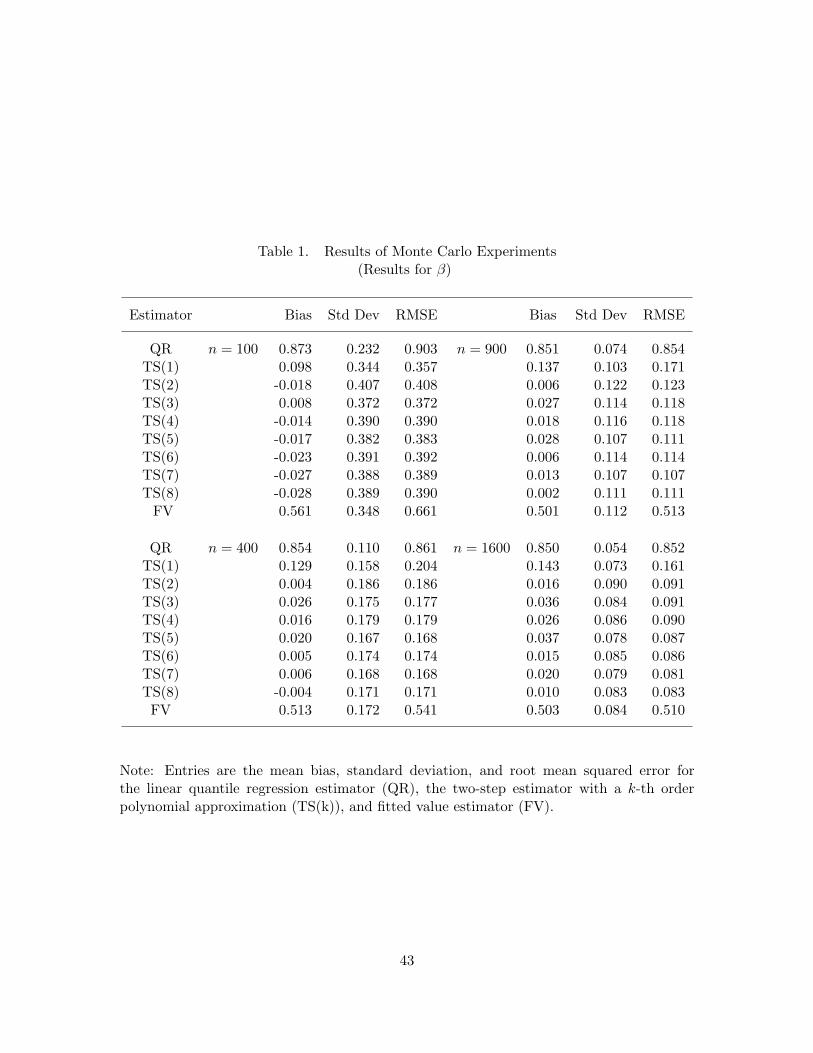
Table 1. Results of Monte Carlo Experiments(Results for β)

Estimator Bias Std Dev RMSE Bias Std Dev RMSE

QR n = 100 0.873 0.232 0.903 n = 900 0.851 0.074 0.854TS(1) 0.098 0.344 0.357 0.137 0.103 0.171TS(2) -0.018 0.407 0.408 0.006 0.122 0.123TS(3) 0.008 0.372 0.372 0.027 0.114 0.118TS(4) -0.014 0.390 0.390 0.018 0.116 0.118TS(5) -0.017 0.382 0.383 0.028 0.107 0.111TS(6) -0.023 0.391 0.392 0.006 0.114 0.114TS(7) -0.027 0.388 0.389 0.013 0.107 0.107TS(8) -0.028 0.389 0.390 0.002 0.111 0.111

FV 0.561 0.348 0.661 0.501 0.112 0.513

QR n = 400 0.854 0.110 0.861 n = 1600 0.850 0.054 0.852TS(1) 0.129 0.158 0.204 0.143 0.073 0.161TS(2) 0.004 0.186 0.186 0.016 0.090 0.091TS(3) 0.026 0.175 0.177 0.036 0.084 0.091TS(4) 0.016 0.179 0.179 0.026 0.086 0.090TS(5) 0.020 0.167 0.168 0.037 0.078 0.087TS(6) 0.005 0.174 0.174 0.015 0.085 0.086TS(7) 0.006 0.168 0.168 0.020 0.079 0.081TS(8) -0.004 0.171 0.171 0.010 0.083 0.083FV 0.513 0.172 0.541 0.503 0.084 0.510

Note: Entries are the mean bias, standard deviation, and root mean squared error forthe linear quantile regression estimator (QR), the two-step estimator with a k-th orderpolynomial approximation (TS(k)), and fitted value estimator (FV).

43

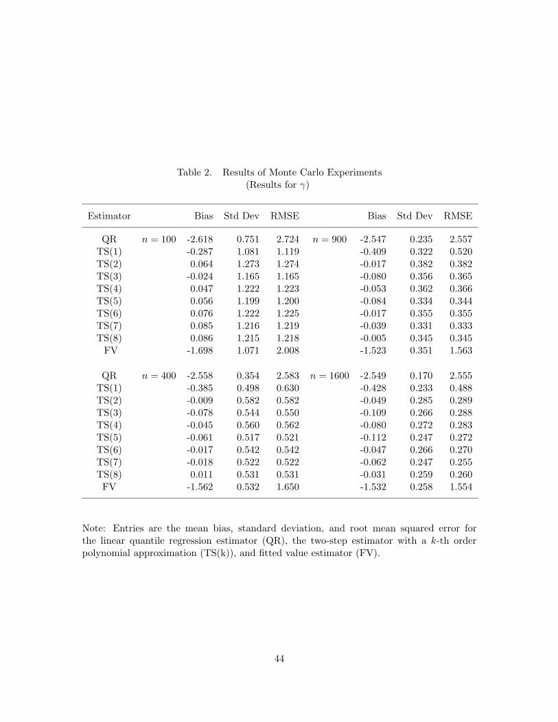
Table 2. Results of Monte Carlo Experiments(Results for γ)

Estimator Bias Std Dev RMSE Bias Std Dev RMSE

QR n = 100 -2.618 0.751 2.724 n = 900 -2.547 0.235 2.557TS(1) -0.287 1.081 1.119 -0.409 0.322 0.520TS(2) 0.064 1.273 1.274 -0.017 0.382 0.382TS(3) -0.024 1.165 1.165 -0.080 0.356 0.365TS(4) 0.047 1.222 1.223 -0.053 0.362 0.366TS(5) 0.056 1.199 1.200 -0.084 0.334 0.344TS(6) 0.076 1.222 1.225 -0.017 0.355 0.355TS(7) 0.085 1.216 1.219 -0.039 0.331 0.333TS(8) 0.086 1.215 1.218 -0.005 0.345 0.345

FV -1.698 1.071 2.008 -1.523 0.351 1.563

QR n = 400 -2.558 0.354 2.583 n = 1600 -2.549 0.170 2.555TS(1) -0.385 0.498 0.630 -0.428 0.233 0.488TS(2) -0.009 0.582 0.582 -0.049 0.285 0.289TS(3) -0.078 0.544 0.550 -0.109 0.266 0.288TS(4) -0.045 0.560 0.562 -0.080 0.272 0.283TS(5) -0.061 0.517 0.521 -0.112 0.247 0.272TS(6) -0.017 0.542 0.542 -0.047 0.266 0.270TS(7) -0.018 0.522 0.522 -0.062 0.247 0.255TS(8) 0.011 0.531 0.531 -0.031 0.259 0.260FV -1.562 0.532 1.650 -1.532 0.258 1.554

Note: Entries are the mean bias, standard deviation, and root mean squared error forthe linear quantile regression estimator (QR), the two-step estimator with a k-th orderpolynomial approximation (TS(k)), and fitted value estimator (FV).

44

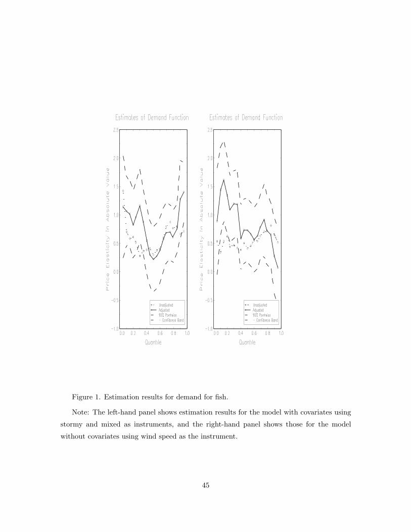
Figure 1. Estimation results for demand for fish.

Note: The left-hand panel shows estimation results for the model with covariates using

stormy and mixed as instruments, and the right-hand panel shows those for the model

without covariates using wind speed as the instrument.

45

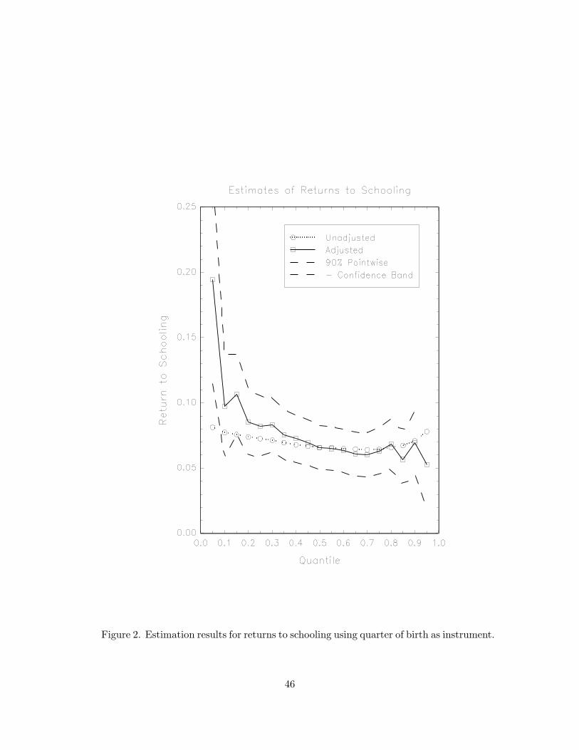
Figure 2. Estimation results for returns to schooling using quarter of birth as instrument.

46

Documents

Endogeneity in Quantile Regression Models: A Control ...fm · PDF fileEndogeneity in Quantile Regression Models: A Control Function Approach ... Endogeneity in Quantile Regression