Embed Size (px)
Citation preview
Iraqi Journal of Statistical Science (32) 2020
P.P [132-149]
A comparison among robust estimation methods for structural equations modeling
with ordinal categorical variables
Omar Salam Ibrahim* Dr Mohammed Jasim Mohammed**
[email protected] [email protected]
Abstract
Categorical and ordered variables are commonly used in many scientific
researches. Researchers often use the ML method, which assumes a multivariate normal
distribution, and this is not true with categorical data because the normal state assumption
is violated when a Likert scale is used which leads to shaded results.
In this research, it has been suggested the robust MLR method with covariance
matrix of the sample which deals with the data as it is a continuous data especially when
the Likert scale is five or above. It has been suggested a method for reducing the error by
linking error measurement, where a link was performed between three standard errors,
and through the fit indices, it was obtained a good result in reducing the standard error of
capabilities and improving the quality of fit indexes. It has been also used two of the
robust methods, WLSMV method which known as RDWLS method, and ULSMV
method which known as RULS method, use a polychoric correlation, each two methods
deal with the data as it categorical. This research also included a comparison between
the robust estimation methods ML , MLR , WLSMV and ULSMV and study its effects
on the population corrected robust model fit indexes , and then select the best method for
dealing with the categorical ordered data . The results showed a superiority of the robust
methods in comparison with other methods, where it showed a robust corrections in the
standard errors by using the polychoric correlation coefficient matrix, in addition to
robust correction of the chi square. In addition of that, the fit indices is replaced by the
robust fit indexes of chi- square robust, TLI, CFI and RMSIA. Keywords: structural equations modeling, robust estimation, Ordered Categorical
Variables, fit indices, This is an open access article under the CC BY 4.0 license
http://creativecommons.org/licenses/by/4.0/)
ملخص:ال
تستخدم المتغيرات الرتبية عمى نطاق واسع في العديد من البحوث وفي كافة التخصصات والتي تفترض التوزيع الطبيعي MLالعممية ، وغالبا ما يستخدم الباحثون طريقة الامكان الاعظم
متعدد المتغيرات ، وهذا ليس صحيحا مع البيانات الرتبية الفئوية حيث ينتهك افتراض التوزيع الطبيعي في حالة استخدام مقياس ليكرات مما يؤدي الى نتائج مضممة وتضخيم في الخطأ المعياري
. عن تأثير عمى مؤررات المطابقةفضلا * Researcher / College of Computer science and Mathematics / Mosul University.
** University of Baghdad/College of Administration and Economics/ Statistics Department>
Received date:8/8 /2002 Accepted date: 7 /9 / 2020 Published data: 1 /20/ 2020
[133] Iraqi Journal of Statistical Science (32) 2020
الامكان الاعظم الحصينة مع مصفوفة التغاير MLRفقد تضمن هذا البحث اقتراح طريقة لمعينة التي تتعامل مع البيانات عمى انها مستمرة وخاصة عندما يكون مقياس ليكرات خماسي فما
ث فوق. وتم اقتراح طريقة لتقميل الخطأ من خلال ربط الاخطاء ، حيث تم اجراء ارتباط بين ثلااخطاء قياسية ، ومن خلال مؤررات التعديل تم الحصول عمى نتائج جيدة في تقميل الخطأ المعياري
وتحسين جودة المطابقة لممؤررات.او مايعرف بطريقة WLSMVكما وتم استخدام طريقتين من الطرق الحصينة ، طريقة RDWLS وطريقةULSMV او مايعرف بطريقةRULS ارتباط متعدد الالوان مع مصفوفة
Polychoric correlation وكمتا الطريقتين تتعامل مع البيانات عمى انها بيانات رتبية . وتضمن ML ،MLR ،WLSMV ،ULSMVالبحث ايضا اجراء مقارنة بين طرق التقدير الحصينة
فضل لمتعامل مع ودراسة تاثيراتها عمى مؤررات المطابقة الحصينة ومن ثم اختيار الطريقة الا WLSMV ،ULSMVالبيانات الرتبية ، وقد تم التوصل الى نتائج جيدة لكل من الطريقتين
مقارنة مع نتائج الطرق الاخرى ، حيث اظهرت النتائج تصحيحات حصينة في الاخطاء المعيارية ت الحصينة عن طريق استخدام مصفوفة معامل الارتباط متعددة الالوان بالاضافة الى التصحيحا
فضلا عن ذلك فان مؤررات المطابقة تم استبدالها بمؤررات المطابقة الحصينة كاي سكوير. لمؤرر . RMSIAو CFI و TLIلكاي سكوير
نمذجة المعادلات الهيكمية ، المتغيرات الرتبية الفئوية ،المقدرات الحصينة، : المفتاحيةكممات ال .مؤررات المطابقة
1. introduction
Many scientists or researchers have discussed different estimation methods for
modeling structural equations, where Assumed theoretical models include free
parameters that we need to estimate, including modeling latent factors, measurement
errors, and factor correlations if it is a Measurement model. If the model is structural, the
estimated parameters reflect the correlations between basic independent variables and the
paths that link the complete independent variables.
The statistical methods that social scientists often use are generally called the
first generation techniques. Which involves regression-based approaches such as multiple
regression, logistic regression and variance analysis, other tools such as first generation
exploratory and confirmatory component analysis, cluster analysis and multidimensional
scaling techniques. Nevertheless, many researchers have more increasingly turned to
second-generation approaches over the past 20 years to resolve the shortcomings of first-
generation methods. researchers introduce non-observable variables or Latent variables
that are evaluated indirectly by observed indices. We also make measurement errors in
measured variables easier to account for.
A comparison among robust estimation methods … [134]
2. objective of research
Using robust methods to estimate the parameters in SEM when the data are in
ordinal categorical and no normal distribution.Choosing the best way for deal with the
ordinal categorical data when we have a five- Likert scale through the estimator that deal
with the data as it is a continuous and the robust estimator that deal with the data as it is
an ordinal categorical. Study the correcting estimator of robust methods. Measuring the
impact of the estimation methods on conformity fit indicators when using the robust Chi
Square Correction for Muthen (2010), the corresponding fit indicators for each CFI, TLI,
RMSEA are all dependent on the Chi Square robust and are replaced by the new Chi-
Square value, the fit indicators are called robust model fit index, and thus it is compared
The effest of robust estimation methods on the robust fit indicators. Suggesting a method
to reduce the error by making a correlation between the standard errors of the variables,
where as the fit indicators give several suggestions to improve the fit of conformity, and a
variation was made between covariance Z62 ~~ Z72 and Z92 ~~ Z102 and Y11 ~~ Y21
3. Ordered Categorical Variables
Ordered categorical variable involves more than two categories. Pearson (1901)
has a long history of analysis and work of polychoric and polyserial correlations, (Li, Li
and Li, 2014). When the data is ordered and categorical, the association measures differ
from those for continuous variables. A common definition for ordered categorical
variables is that an ordered categorical variable is classified into the observed ordinal
variable through applying a number of thresholds.The relationship is called tetrachoric
correlation with two underlying continuous variables, while the calculated variables are
binary. The resulting correlation is called polychoric association, if the calculated
variables have more than two classes.
One way in which observed ordered categorical results occur by dividing a continuous,
normally distributed latent response variable (y*) into differentcategories (e.g., Bollen,
1989). Thresholds (t) are the points which divide the continuous latent response variable
(y*) into a set number of categories (c) where the total number of thresholds is equal to
the number of categories less one (c – 1).where ∞ is The
relationship between a latent response distribution, y*, with an observed ordinal
distribution, y, is formalized as
The observed ordinal value for y changes if a threshold on the latent response
variable y * is exceeded . For example, if a Likert scale has five response choices, it will
require four threshold values to divide y * into five ordered categories. The ordinal data
(y) observed is thought to be t
{
}
Usually, polychoric correlations are computed using the two-stage method Olsson
(1979) defined. (Flora and Curran, 2004) (Course, 2013)
4. Building structural model The fundamental building blocks of SEM analyzes are implemented using a
sequential series of five phases or processes: model definition, model identification, model
[135] Iraqi Journal of Statistical Science (32) 2020
estimation, model checking and model adjustment. Such fundamental building blocks are
utterly necessary for SEM models to be carried out. Wang (2020)
4.1 Modeling of Structural Equation (SEM)
SEM of two basic sets of models: the measuring model and the model structure , uses
the confirmatory factor analysis ( CFA) to form the latent variables (factors) and adjust the
measuring error of the indicator . The exogenous indicator x measurement model and the
endogenous indicators y can be described as
The structural model is defined as
where and are Described as the latent variables vectors given above, is the
matrix of Coefficients of regression between the latent endogenous variables,
and is the Coefficients of SR regression matrix among latent endogenous and
exogenous variables, is the vector with observed residual
The covariance matrix is obtained as follows
(4)
Therefore the matrix of covariance was proven. (Timm, no date)
4.2 Estimation of Model Parameters
Estimation is a technique for calculating unknown parameters by optimizing the
basic fit function consisting of the hypothesized model and the data observed, Estimation
is basically the most important aspect for analysis including methods estimation
following
4.2.1 Maximum likelihood function for SEM (ML)
Maximum Likelihood (ML) is the most commonly used fit function for structural
equations modeling . Almost every software programs uses ML as their main estimator .
This approach , leads to estimates of the parameters which increase the likelihood to
obtaining the covariance matrix empirical S. from implied covariance matrix model .
The minimized log Likelihood possibility function log L is (Bollen, 1989)
In this case, MLE function can be defined as in equation (5).
(5)
Where q is X variable number and p is Y variable number. Where is a parameter
vector.
is a covariance matrix model implied . is The fitting function value
measured at the estimates final. determinant. tr is the trace of a matrix. (Bollen,
1989) , and Standard errors are the square roots of the diagonal components of the
approximate asymptotic covariance matrix from FML under the multivariate normality
assumption:
(
) * (
)+
where Is the model's partial derivatives matrix as
respects the parameters. The square roots of the diagonal components then the standard
errors. Estimates of parameters provided by ML are desirable asymptotic, such as
A comparison among robust estimation methods … [136]
unbiased, consistency and efficiency in addition the test statistics which use Wishart's
probability are described as
, (7)
or follows a distribution with degrees of freedom, where represents
the number of non-duplicated elements in the observed covariance matrix , whiel the number of unknown parameters. (Crisci, 2012) (Bollen, 1989)
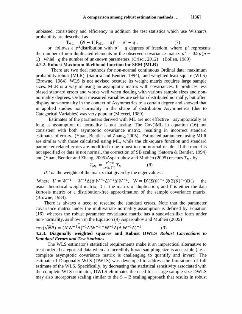
4.2.2. Robust Maximum likelihood function for SEM (MLR)
There are two deal methods for non-normal continuous Ordinal data: maximum
probability robust (MLR) (Satorra and Bentler, 1994), and weighted least square (WLS)
(Browne, 1984). WLS is not advised because its weight matrix requires large sample
sizes. MLR is a way of using an asymptotic matrix with covariances. It produces less
biased standard errors and works well when dealing with various sample sizes and non-
normality degrees. Ordinal measured variables are seldom distributed normally, but often
display non-normality in the context of Asymmetrics to a certain degree and showed that
in applied studies non-normality in the shape of distribution Asymmetrics (due to
Categorical Variables) was very popular.(Micceri, 1989)
Estimates of the parameters derived with ML are not effective asymptotically as
long as assumption of normality is not lasting. The Cov()ML in equation (16) not
consistent with both asymptotic covariance matrix, resulting in incorrect standard
estimates of errors.. (Yuan, Bentler and Zhang, 2005) . Estimated parameters using MLR
are similar with those calculated using ML, while the chi-square function and standard
parameter-related errors are modified to be robust to non-normal results. If the model is
not specified or data is not normal, the correction of SB scaling (Satorra & Bentler, 1994)
and (Yuan, Bentler and Zhang, 2005)Asparouhov and Muthén (2005) rescues by
(8)
is the weights of the matrix that given by the eigenvalues .
Where ,
Is the
usual theoretical weight matrix; is the matrix of duplication; and is either the data
kurtosis matrix or a distribution-free approximation of the sample covariance matrix.
(Browne, 1984).
There is always a need to rescalue the standard errors. Note that the parameter
covariance matrix under the multivariate normality assumption is defined by Equation
(16), whereas the robust parameter covariance matrix has a sandwich-like form under
non-normality, as shown in the Equation (9) Asparouhov and Muthén (2005)
√
(9)
4.2.3. Diagonally weighted squares and Robust DWLS Robust Corrections to
Standard Errors and Test Statistics
The WLS estimator's statistical requirements make it an impractical alternative to
treat ordered categorical data when an incredibly broad sampling size is accessible (i.e. a
complete asymptotic covariance matrix is challenging to quantify and invert). The
estimate of Diagonally WLS (DWLS) was developed to address the limitations of full
estimate of the WLS. Specifically, by decreasing the statistical sensitivity associated with
the complete WLS estimator, DWLS eliminates the need for a large sample size DWLS
may also incorporate scaling similar to the S – B scaling approach that results in robust
[137] Iraqi Journal of Statistical Science (32) 2020
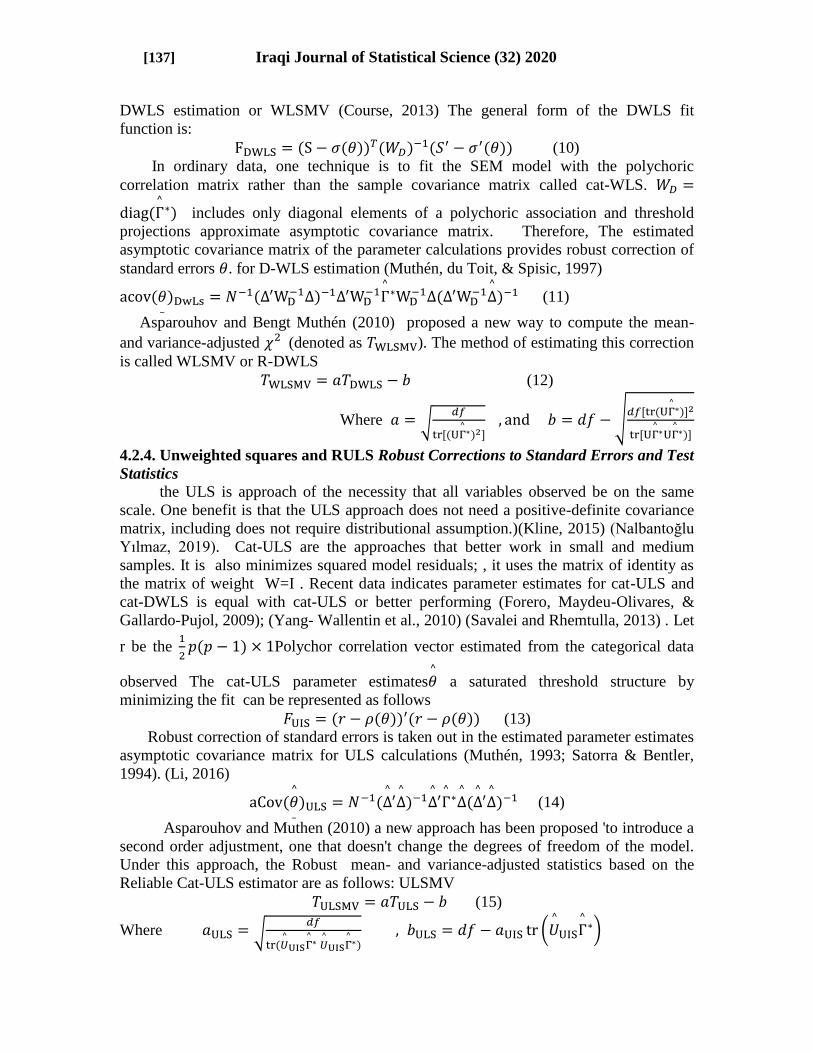
DWLS estimation or WLSMV (Course, 2013) The general form of the DWLS fit
function is:
(10)
In ordinary data, one technique is to fit the SEM model with the polychoric
correlation matrix rather than the sample covariance matrix called cat-WLS.
includes only diagonal elements of a polychoric association and threshold
projections approximate asymptotic covariance matrix. Therefore, The estimated
asymptotic covariance matrix of the parameter calculations provides robust correction of
standard errors . for D-WLS estimation (Muthén, du Toit, & Spisic, 1997)
(11)
Asparouhov and Bengt Muthén (2010) proposed a new way to compute the mean-
and variance-adjusted (denoted as ). The method of estimating this correction
is called WLSMV or R-DWLS
(12)
Where √
√
4.2.4. Unweighted squares and RULS Robust Corrections to Standard Errors and Test
Statistics
the ULS is approach of the necessity that all variables observed be on the same
scale. One benefit is that the ULS approach does not need a positive-definite covariance
matrix, including does not require distributional assumption.)(Kline, 2015) (Nalbantoğlu
Yılmaz, 2019). Cat-ULS are the approaches that better work in small and medium
samples. It is also minimizes squared model residuals; , it uses the matrix of identity as
the matrix of weight W=I . Recent data indicates parameter estimates for cat-ULS and
cat-DWLS is equal with cat-ULS or better performing (Forero, Maydeu-Olivares, &
Gallardo-Pujol, 2009); (Yang- Wallentin et al., 2010) (Savalei and Rhemtulla, 2013) . Let
r be the
Polychor correlation vector estimated from the categorical data
observed The cat-ULS parameter estimates
a saturated threshold structure by
minimizing the fit can be represented as follows
(13)
Robust correction of standard errors is taken out in the estimated parameter estimates
asymptotic covariance matrix for ULS calculations (Muthén, 1993; Satorra & Bentler,
1994). (Li, 2016)
(14)
Asparouhov and Muthen (2010) a new approach has been proposed 'to introduce a
second order adjustment, one that doesn't change the degrees of freedom of the model.
Under this approach, the Robust mean- and variance-adjusted statistics based on the
Reliable Cat-ULS estimator are as follows: ULSMV
(15)
Where √
(
)
A comparison among robust estimation methods … [138]
(Yang-Wallentin, Jöreskog and Luo, 2010) (Xia and Yang, 2018)
4.3 Model evaluation
A main feature of SEM is the performance of an overall model fit test to the basic
hypothesis,Σ(θ)=Σ , the degree for which the model estimation variance covariance
matrix Σ differs with the sample variance covariance matrix observed S However , If
the model-estimated variance covariance matrix, Σ , is non significantly different with the
observed data covariance matrix, S, then we can say the model fits the data well,
otherwise, the null hypothesis was rejected . Bollen 1989; Jöreskog and Sörbom 1989;
Bentler 1990) The estimation of the all model fit will be performed before the parameter
estimates are interpreted ny assumption from the sample estimation may be misleading
without testing the model fit Numerous model fit indices been have developed to
determine the closeness of S to Σ (Bollen,1989)
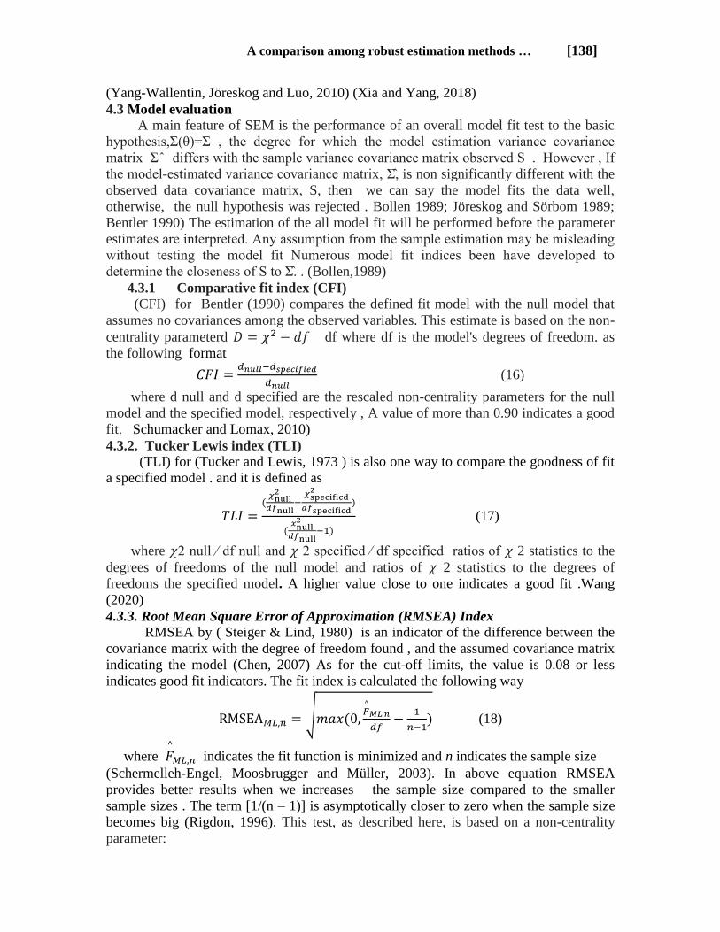
4.3.1 Comparative fit index (CFI) (CFI) for Bentler (1990) compares the defined fit model with the null model that
assumes no covariances among the observed variables. This estimate is based on the non-
centrality parameterd df where df is the model's degrees of freedom. as
the following format
(16)
where d null and d specified are the rescaled non-centrality parameters for the null
model and the specified model, respectively , A value of more than 0.90 indicates a good
fit. Schumacker and Lomax, 2010)
4.3.2. Tucker Lewis index (TLI)
(TLI) for (Tucker and Lewis, 1973 ) is also one way to compare the goodness of fit
a specified model . and it is defined as
(17)
where 2 null ∕ df null and 2 specified ∕ df specified ratios of 2 statistics to the
degrees of freedoms of the null model and ratios of 2 statistics to the degrees of
freedoms the specified model. A higher value close to one indicates a good fit .Wang
(2020)
4.3.3. Root Mean Square Error of Approximation (RMSEA) Index RMSEA by ( Steiger & Lind, 1980) is an indicator of the difference between the
covariance matrix with the degree of freedom found , and the assumed covariance matrix
indicating the model (Chen, 2007) As for the cut-off limits, the value is 0.08 or less
indicates good fit indicators. The fit index is calculated the following way
√
(18)
where
indicates the fit function is minimized and n indicates the sample size
(Schermelleh-Engel, Moosbrugger and Müller, 2003). In above equation RMSEA
provides better results when we increases the sample size compared to the smaller
sample sizes . The term [1/(n – 1)] is asymptotically closer to zero when the sample size
becomes big (Rigdon, 1996). This test, as described here, is based on a non-centrality
parameter:
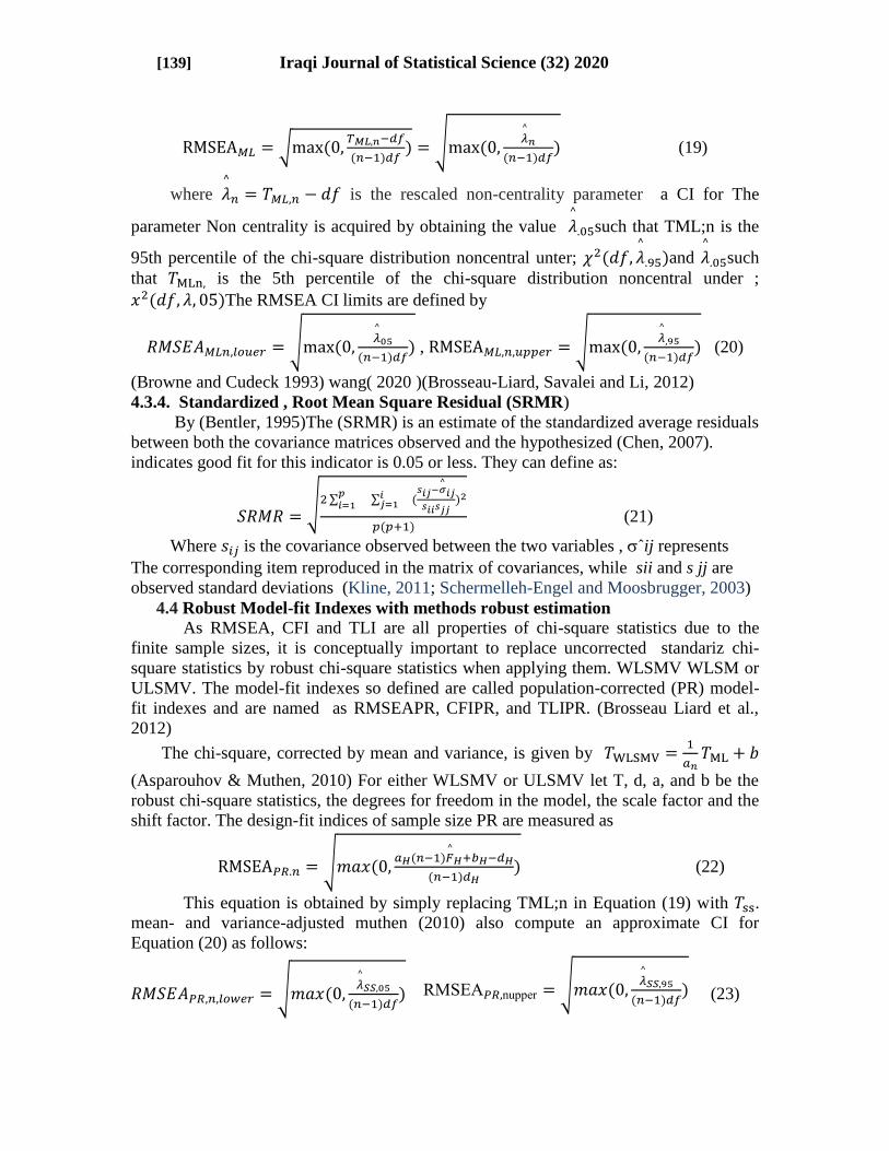
[139] Iraqi Journal of Statistical Science (32) 2020
√
√
(19)
where
is the rescaled non-centrality parameter a CI for The
parameter Non centrality is acquired by obtaining the value
such that TML;n is the
95th percentile of the chi-square distribution noncentral unter;
and
such
that is the 5th percentile of the chi-square distribution noncentral under ;
The RMSEA CI limits are defined by
√
, √
(20)
(Browne and Cudeck 1993) wang( 2020 )(Brosseau-Liard, Savalei and Li, 2012)
4.3.4. Standardized , Root Mean Square Residual (SRMR)
By (Bentler, 1995)The (SRMR) is an estimate of the standardized average residuals
between both the covariance matrices observed and the hypothesized (Chen, 2007).
indicates good fit for this indicator is 0.05 or less. They can define as:
√ ∑
∑
(21)
Where is the covariance observed between the two variables , ˆij represents
The corresponding item reproduced in the matrix of covariances, while sii and s jj are
observed standard deviations (Kline, 2011; Schermelleh-Engel and Moosbrugger, 2003)
4.4 Robust Model-fit Indexes with methods robust estimation
As RMSEA, CFI and TLI are all properties of chi-square statistics due to the
finite sample sizes, it is conceptually important to replace uncorrected standariz chi-
square statistics by robust chi-square statistics when applying them. WLSMV WLSM or
ULSMV. The model-fit indexes so defined are called population-corrected (PR) model-
fit indexes and are named as RMSEAPR, CFIPR, and TLIPR. (Brosseau Liard et al.,
2012)
The chi-square, corrected by mean and variance, is given by
(Asparouhov & Muthen, 2010) For either WLSMV or ULSMV let T, d, a, and b be the
robust chi-square statistics, the degrees for freedom in the model, the scale factor and the
shift factor. The design-fit indices of sample size PR are measured as
√
(22)
This equation is obtained by simply replacing TML;n in Equation (19) with .
mean- and variance-adjusted muthen (2010) also compute an approximate CI for
Equation (20) as follows:
√
RMSE nupper √
(23)
A comparison among robust estimation methods … [140]
(24)
(25)
(Brosseau-liard et al., 2014)(Xia and Yang, 2019)
4.5 Modification indices
The indices of modifications help to classify regions of possible model weakness.
Their usefulness lies in their capacity to prescribe such changes in order to boost the
model's goodness-of-fit. In addition, adjustment indices (provided by all software) will
identify the parameters, which greatly contribute to the fit of the model when applied to
it. Gana (2019)
5. Applied side
In this part, a comparison is made between estimation methods in terms of
parameter estimater , standard error and fit indicators . The model of structural
equations is one of the most methods in that used many fields. the model was applied on
a data of catigorical ordered from the five Likert scale represented by a questionnaire
devoted specified for the the administrative aspect, where the objective of the research is
to use the robust estimation methods especially when we deal with the categorical
ordered data , so the Violation the assumption of normal distirabuation is predominant.
ML is the most common technique available in most programs, Satorra (1998) suggested
methods for correcting statistics and standard errors to a degree commensurate with the
multivariate kurtosis of the observed data.
An applied study was carried out by relying on data from a doctoral thesis for a
field study within the University of Mosul, represented by strategic communication
patterns and their reflection in building dynamic capabilities A questionnaire Questions,
Mosul University Professors (Ayman, 2019) . Taking part of the scale and constructing a
model consisting of 6 latent variables (dimensions) where the latent variable y1
represents the sharing of knowledge. A process by which the organization looks to be
creative with the products it provides to its customers. The latent variable y2 brand is the
sum total of the banana of the organization that passed to the different audiences of the
organization. The latent variable y3 represents the polarization of external knowledge,
Gain knowledge from outside the organization (market, research centers, and
universities). These three variables operate as latent Exogenous (independent) variables.
As for the latent mediation variables, they are represented by Z1: how efficient the
integration in which the organization has access to the knowledge that its subsidiaries
have. The second latent variable is the mediation Z2, the flexibility of integration
represents the multiplicity and type of knowledge areas that the organization possesses
and from which it derives its capabilities, while Y1 represents the approved endogenous
variable, repair, the organization's ability to learn from its previous experiences and the
experiences of other organizations. . the study represented 32 observational variables that
represent the paragraphs of the questionnaire distributed among the latent changes, which
are not seen. The sample size was 384 views. Modeling requires a sample size greater
than 200. One of the well-known rules in the field of determining the least sample size is
what Jackson has proposed around the base of q: N , q represents the number of
parameters that need to be estimated relative to the sample size for N, and suggested
[141] Iraqi Journal of Statistical Science (32) 2020
method two is the number of observe N to the number of variables p , as the sample size
is suitable for conducting the study when 10 <(N/p) (1/10), i.e. 10 for each variable at
least .Jackson(2003)
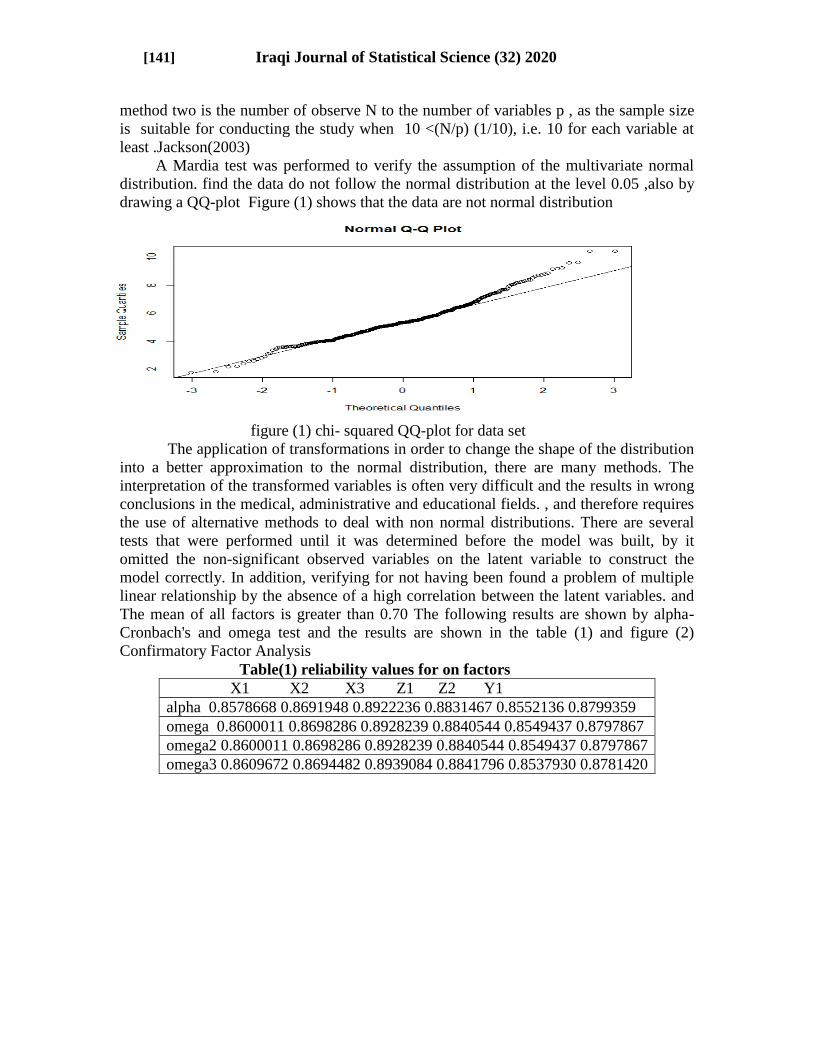
A Mardia test was performed to verify the assumption of the multivariate normal
distribution. find the data do not follow the normal distribution at the level 0.05 ,also by
drawing a QQ-plot Figure (1) shows that the data are not normal distribution
figure (1) chi- squared QQ-plot for data set
The application of transformations in order to change the shape of the distribution
into a better approximation to the normal distribution, there are many methods. The
interpretation of the transformed variables is often very difficult and the results in wrong
conclusions in the medical, administrative and educational fields. , and therefore requires
the use of alternative methods to deal with non normal distributions. There are several
tests that were performed until it was determined before the model was built, by it
omitted the non-significant observed variables on the latent variable to construct the
model correctly. In addition, verifying for not having been found a problem of multiple
linear relationship by the absence of a high correlation between the latent variables. and
The mean of all factors is greater than 0.70 The following results are shown by alpha-
Cronbach's and omega test and the results are shown in the table (1) and figure (2)
Confirmatory Factor Analysis
Table(1) reliability values for on factors
X1 X2 X3 Z1 Z2 Y1
alpha 0.8578668 0.8691948 0.8922236 0.8831467 0.8552136 0.8799359
omega 0.8600011 0.8698286 0.8928239 0.8840544 0.8549437 0.8797867
omega2 0.8600011 0.8698286 0.8928239 0.8840544 0.8549437 0.8797867
omega3 0.8609672 0.8694482 0.8939084 0.8841796 0.8537930 0.8781420
A comparison among robust estimation methods … [142]
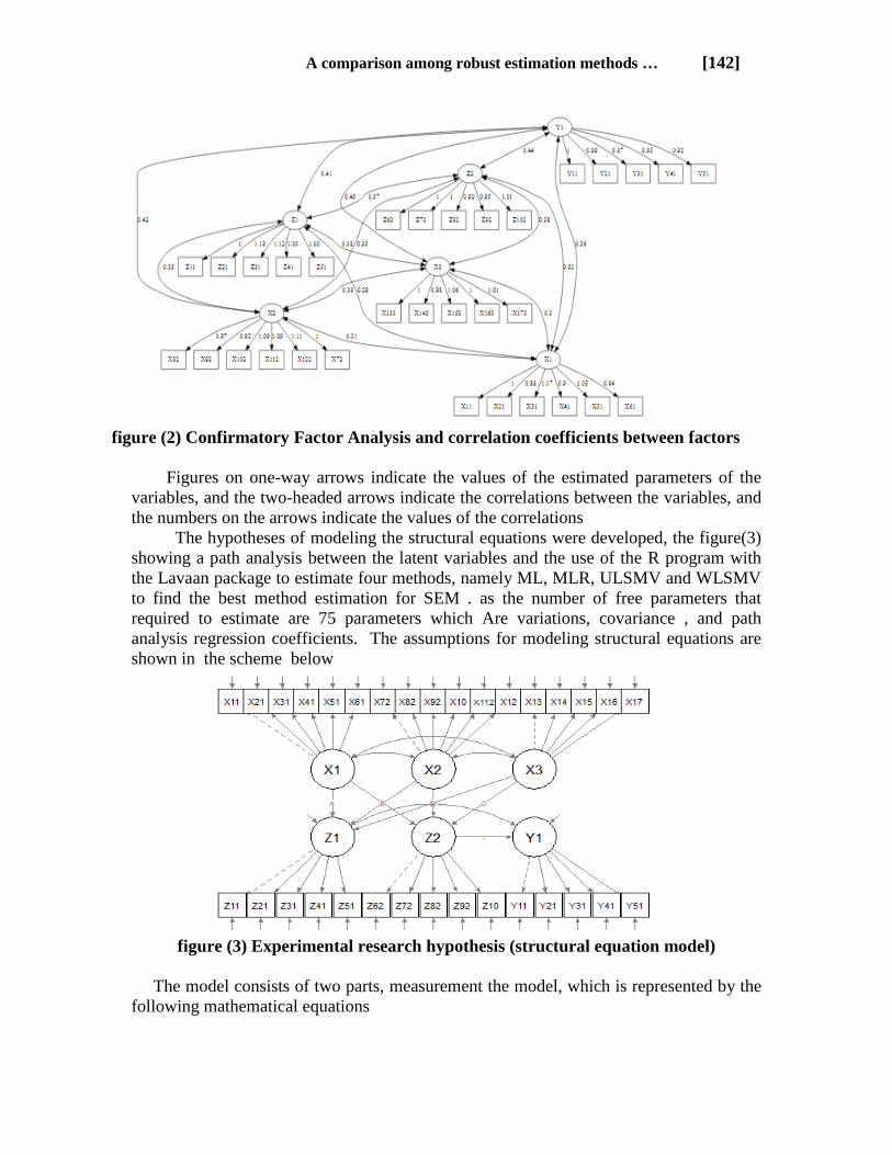
figure (2) Confirmatory Factor Analysis and correlation coefficients between factors
Figures on one-way arrows indicate the values of the estimated parameters of the
variables, and the two-headed arrows indicate the correlations between the variables, and
the numbers on the arrows indicate the values of the correlations
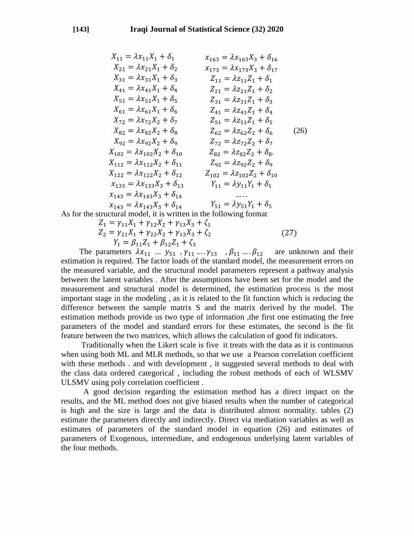
The hypotheses of modeling the structural equations were developed, the figure(3)
showing a path analysis between the latent variables and the use of the R program with
the Lavaan package to estimate four methods, namely ML, MLR, ULSMV and WLSMV
to find the best method estimation for SEM . as the number of free parameters that
required to estimate are 75 parameters which Are variations, covariance , and path
analysis regression coefficients. The assumptions for modeling structural equations are
shown in the scheme below
figure (3) Experimental research hypothesis (structural equation model)
The model consists of two parts, measurement the model, which is represented by the
following mathematical equations
[143] Iraqi Journal of Statistical Science (32) 2020
(26)
As for the structural model, it is written in the following format
The parameters ... , , are unknown and their
estimation is required. The factor loads of the standard model, the measurement errors on
the measured variable, and the structural model parameters represent a pathway analysis
between the latent variables . After the assumptions have been set for the model and the
measurement and structural model is determined, the estimation process is the most
important stage in the modeling , as it is related to the fit function which is reducing the
difference between the sample matrix S and the matrix derived by the model. The
estimation methods provide us two type of information ,the first one estimating the free
parameters of the model and standard errors for these estimates, the second is the fit
feature between the two matrices, which allows the calculation of good fit indicators.
Traditionally when the Likert scale is five it treats with the data as it is continuous
when using both ML and MLR methods, so that we use a Pearson correlation coefficient
with these methods . and with development , it suggested several methods to deal with
the class data ordered categorical , including the robust methods of each of WLSMV
ULSMV using poly correlation coefficient .
A good decision regarding the estimation method has a direct impact on the
results, and the ML method does not give biased results when the number of categorical
is high and the size is large and the data is distributed almost normality. tables (2)
estimate the parameters directly and indirectly. Direct via mediation variables as well as
estimates of parameters of the standard model in equation (26) and estimates of
parameters of Exogenous, intermediate, and endogenous underlying latent variables of
the four methods.
A comparison among robust estimation methods … [144]
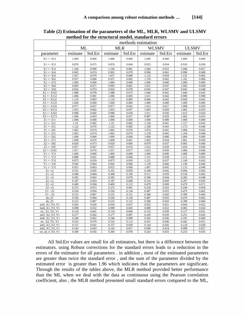
Table (2) Estimation of the parameters of the ML, MLR, WLSMV and ULSMV
method for the structural model, standard errors
methods estimation
ULSMV WLSMV MLR ML
Std.Err estimate Std.Err estimate Std.Err estimate Std.Err estimate parameter 0.000 1.000 0.000 1.000 0.000 1.000 0.000 1.000 X1 =~ X11
0.058 0.910 0.054 0.923 0.064 0.876 0.075 0.876 X1 =~ X21
0.057 1.046 0.052 1.046 0.081 1.166 0.090 1.166 X1 =~ X31
0.068 0.998 0.061 0.996 0.078 0.902 0.074 0.902 X1 =~ X41
0.065 1.132 0.059 1.122 0.080 1.057 0.079 1.057 X1 =~ X51
0.068 1.181 0.062 1.159 0.082 0.937 0.080 0.937 X1 =~ X61
0.000 1.000 0.000 1.000 0.000 1.000 0.000 1.000 X2 =~ X72
0.038 1.042 0.037 1.051 0.061 0.983 0.071 0.983 X2 =~ X82
0.048 0.945 0.047 0.945 0.078 0.924 0.074 0.924 X2 =~ X92
0.043 1.040 0.042 1.046 0.075 1.088 0.078 1.088 X2 =~ X102
0.998
0.044
0.998
0.044
0.042 1.011 0.085 1.086 0.081 1.086 X2 =~ X112
0.042 0.949 0.042 0.960 0.083 1.110 0.083 1.110 X2 =~ X122
0.000 1.000 0.000 1.000 0.000 1.000 0.000 1.000 X3 =~ X133
0.029 1.008 0.027 1.015 0.042 0.977 0.057 0.977 X3 =~ X143
0.033 1.002 0.029 1.005 0.057 1.053 0.062 1.053 X3 =~ X153
0.034 1.013 0.030 1.011 0.058 0.988 0.060 0.988 X3 =~ X163
0.033 1.002 0.029 0.987 0.057 1.006 0.063 1.006 X3 =~ X173
0.000 1.000 0.000 1.000 0.000 1.000 0.000 1.000 Z1 =~ Z11
0.043 1.127 0.041 1.128 0.082 1.19 0.082 1.19 Z1 =~ Z21
0.046 1.173 0.043 1.168 0.082 1.122 0.076 1.122 Z1 =~ Z31
0.043 1.064 0.041 1.076 0.076 1.062 0.074 1.062 Z1 =~ Z41
0.048 1.164 0.045 1.159 0.079 1.062 0.074 1.062 Z1 =~ Z51
0.000 1.000 0.000 1.000 0.000 1.000 0.000 1.000 Z2 =~ Z62
0.036 1.001 0.034 1.003 0.047 1.009 0.070 1.009 Z2 =~ Z72
0.040 0.905 0.037 0.879 0.060 0.929 0.073 0.929 Z2 =~ Z82
0.046 1.050 0.039 1.025 0.076 0.957 0.067 0.957 Z2 =~ Z92
0.046 1.084 0.039 1.025 0.077 1.017 0.070 1.017 Z2 =~ Z102
0.000 1.000 0.000 1.000 0.000 1.000 0.000 1.000 Y1 =~ Y11
0.043 1.151 0.038 1.131 0.046 0.888 0.061 0.888 Y1 =~ Y21
0.043 1.149 0.037 1.121 0.050 0.875 0.059 0.875 Y1 =~ Y31
0.046 1.156 0.040 1.129 0.060 0.945 0.064 0.945 Y1 =~ Y41
0.049 1.115 0.042 1.097 0.060 0.925 0.063 0.925 Y1 =~ Y51
0.043 0.094 0.042 0.108 0.059 0.101 0.045 0.101 Z1 ~x1
0.063 0.536 0.059 0.511 0.109 0.498 0.084 0.498 Z1 ~x2
0.048 0.285 0.044 0.296 0.078 0.283 0.062 0.283 Z1 ~x3
0.050 0.207 0.049 0.210 0.068 0.187 0.054 0.187 Z2 ~x1
0.071 0.479 0.069 0.478 0.122 0.469 0.094 0.469 Z2 ~x2
0.058 0.249 0.055 0.259 0.091 0.272 0.072 0.272 Z2 ~x3
0.062 0.470 0.055 0.487 0.136 0.556 0.094 0.556 Y1 ~ Z1
0.060 0.399 0.050 0.380 0.131 0.525 0.087 0.525 Y1 ~ Z2
0.062 0.470 0.055 0.487 0.136 0.556 0.094 0.556 dir_Z1
0.060 0.399 0.050 0.380 0.131 0.525 0.087 0.525 dir_Z2
0.022 0.044 0.021 0.052 0.037 0.056 0.026 0.056 ind1_X1_TO_Y1
0.024 0.083 0.022 0.080 0.045 0.098 0.032 0.098 Ind2_X1_TO_Y1
0.031 0.127 0.030 0.132 0.060 0.154 0.041 0.154 tot _X1_TO_Y1
0.043 0.251 0.039 0.249 0.087 0.277 0.062 0.277 ind1_X2_TO_Y1
0.040 0.191 0.036 0.182 0.088 0.246 0.062 0.246 Ind2_X2_TO_Y1
0.051 0.442 0.048 0.431 0.113 0.523 0.079 0.523 tot _X2_TO_Y1
0.028 0.134 0.026 0.144 0.058 0.157 0.042 0.157 ind1_X3_TO_Y1
0.027 0.099 0.024 0.099 0.057 0.143 0.043 0.143 Ind2_X3_TO_Y1
0.035 0.233 0.033 0.243 0.078 0.300 0.056 0.300 tot_nd_4_TO_Y1
All Std.Err values are small for all estimators, but there is a difference between the
estimators. using Robust corrections for the standard errors leads to a reduction in the
errors of the estimator for all parameters . in addition , most of the estimated parameters
are greater than twice the standard error , and the sum of the parameter divided by the
estimated error is greater than 1.96 which indicates that the parameters are significant.
Through the results of the tables above, the MLR method provided better performance
than the ML when we deal with the data as continuous using the Pearson correlation
coefficient, also , the MLR method presented small standard errors compared to the ML,
[145] Iraqi Journal of Statistical Science (32) 2020
where as the estimation method is the same but the correction in the robust standard
errors As a result, the corresponding fit indicators provided a perfect match compared
with the way ML method, so it is preferable to use MLr with the ordered catigorical data
that does not normal distribution
We also note from the table of estimators WLSMV, ULSMV robust, a significant
improvement in the values of parameter estimates and standard errors. Where as the
errors less than methods ML, MLR using polycoric correlation coefficient with
wlsmv,ulsmv. Although small results were obtained for standard errors for each
estimator by wlsmv, ulsmv, but fit indicators for a ulsmv provided better performance
than a wlsmv.Based on the results of the above methods we recommend to use the
ULSMV method , for this reason also will be explained the robust ulsmv estimation
method in reserch.
By analyzing the results of the model and setting research hypotheses based on
theory, there is an indirect effect of the latent Exogenous variables through the mediation
latent variables on the endogenous latent variable , and there is no direct effect on the
relationship , and there is complete mediation as we note through the application.
Table (2) shows parameter estimates for the ULSMV estimator as there is a direct
effect from the Exogenous latent variable for each x1 x2 x3 which represented by
knowledge and brand sharing and knowledge polarization on the mediation variable Z1
the adequacy of integration .also, there is an effect on the second mediation variable
flexibility of integration Z2 , and all the track effects were significant, achieving the
results of the model hypothesis. Also, there was a direct effect by the two mediation
variables, Z1 and Z2, on the endogenous variable, Y1 learning.
Through the two mediation variables, there is an indirect provocation of the
Exogenous latent variables X1 X2 X3 by the mediation variable Z1, and at the same time
there is an indirect effect from the Exogenous latent variables X1 X2 X3 to the
endogenous latent variable Y1 by the second mediation variable Z2 ,so that the amount of
indirect effect X1 to Y1 by the mediation variable Z1 is 0.44 with a standard error of
0.22.
There is an indirect effect from the variable X1 to Y1 via the second mediation
variable variable Z2 which is 0.83 and with a standard error of 0.24 ,while the overall
effect of X1 across each of the two mediation variables Z1 Z2 to Y1 is 0.127 with a
standard error of 0.31. in the same Method, the effect of the direct and indirect pathway
of both X2 to Y1 was studied by the two mediation potential variables Z1 Z2, as well as
X3 to Y1 via Z1 Z2 where as all values were significant and errors were small.
5.1 Classical and robust fit indicesr
The main types of fit indicators were presented, and the assumed sem model was
examined from the perspective of different estimation methods. We note that the model
estimated according to ML methods obtained good fit indicators, while the RMSEA TLI
CFI SRMR indicators was within the ideal interval, and the model estimated under the
MLR method obtained higher quality fit indicators than the ML, especially when using
the Yuan- Bentler, and the scaling correction factor was 1.218. By dividing this value on
the standard Chi Square value of ML we get the robust corrected value which is 834.945,
and since the fit indicators for RMSEA TLI CFI depend on the chi-Square corrector, it
replaced the value of the robust chi-Square and leads to an improvement in the fit
indicators of the conformity.
A comparison among robust estimation methods … [146]
As for the conformance fit indicesr of the WLSMV method using the robust
Chi Square Correction Factor for Muthén 2010 , when we deal with the data categorical
ordinal and the polycoric correlation coefficient , the value of Chi Square is 1127.826,
while the correction value was equal to Scaling correction factor = 248.365 and shift
parameter is 0.971. the fit indicators for the ULSM estimator with Muthén correction
2010 , provided superior performance in model fit for all conformance indicators when
we deal with categorical data. therefore, we recommend using the ULSMV estimator
when the data is ordinal with Likert scale categorical data, contrary to what most
researchers use with Common ML estimator in most programs.
From this results , we conclude that the best fit of data when we deal with the data
as it is continuous using MLR robust, where as the robust estimator provides a correction
in the kurtosis of resulting from the lack of a normal distribution of data, and most of the
fit robust indicators performed better than the ML fit indicators, As for the WLSMV
ULSMV estimators, the strong fit indicators for the ULSMV estimator provided an
optimal fit performance better than the WLSMV when dealing with the data as orderd
catigorical by correction in the mean and variance . table(4) shows the fit indicators for
the methods.
Table (3) indicators of classical and robust fit of the four estimators
TLI CFI SRMR upper lower RMSEA
df Chi Square estimator
0.917 0.924 0.047 0.062 0.052 0.057 2.244 453 1016.830 ML
0.929 0.935 0.047 0.051 0.042 0.047 1.843 453 834.945 MLR
0.950 0.954 0.045 0.067 0.058 0.062 2.489 453 1127.826 WLSMV
0.951 0.955 0.045 0.061 0.051 0.056 2.202 453 997.628 ULSMV
5.2 fit indicators of classic and robust fit after adjusting for errors between observed
variables
We note through the fit indicators before and after making the covariance between
measurement errors Z62 ~~ Z72 and Z92 ~~ Z102 and Y11 ~~ Y21, there is
improvement in all indicators for all methods , as the values of the Chi Square have
decreased and the values of the root mean square error of approximation index decreased
close to 0.05 and less .this indicates that the index is within the good interval, as the
closer to zero the greater the strength of fit to the model and the value falls within the
interval of confidence accepted. In addition to to that, it has been shown increasing in the
values of CFI and TLI indicators and its approached one. the value of the SRMR index
which is based on the analysis of the standard residual matrix, when ever close to zero
indicates a good match and less influence with the parameters of the chi-Square.
Table (4) indicators of classical and robust fit of the four estimators after
Adjustment
TLI CFI SRMR upper lower RMSEA
df Chi-square estimator
0.934 0.940 0.045 0.055 0.046 0.051 1.984 450 892.994 ML
0.948 0.953 0.045 0.051 0.039 0.045 1.633 450 734.921 MLR
0.958 0.962 0.043 0.062 0.052 0.057 2.238 450 1007.141 WLSMV
0.959 0.963 0.043 0.058 0.049 0.053 2.091 450 941.117 ULSMV
[147] Iraqi Journal of Statistical Science (32) 2020
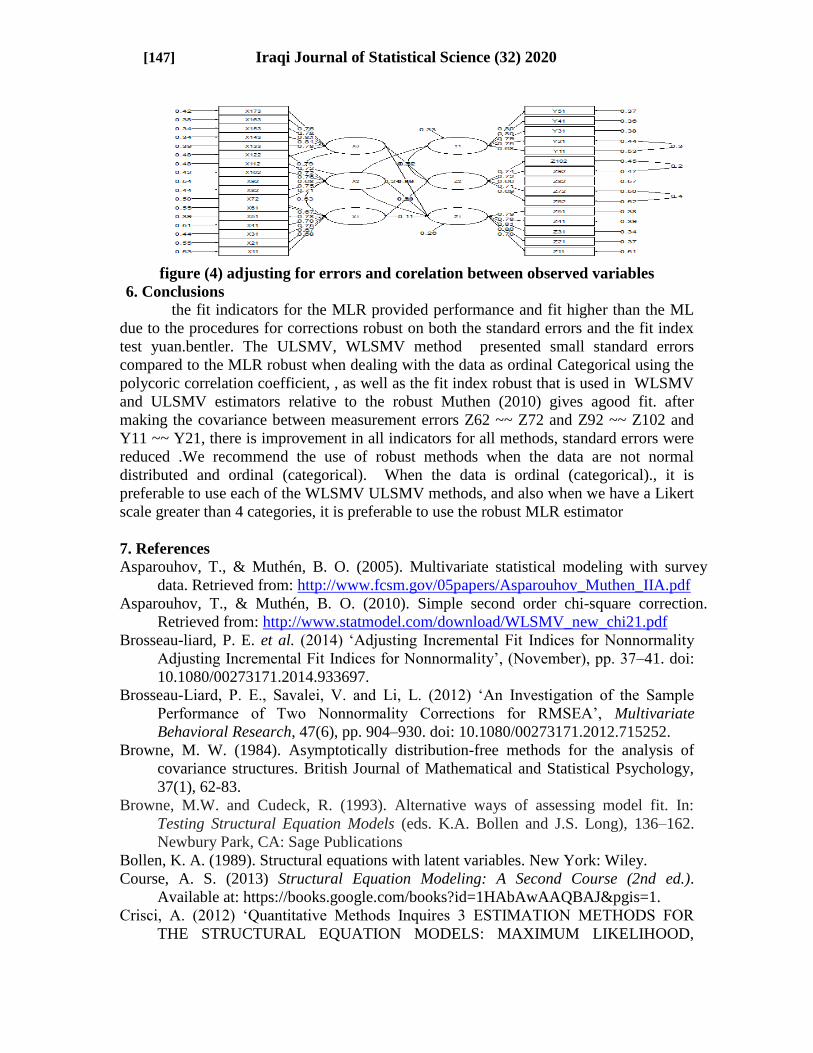
figure (4) adjusting for errors and corelation between observed variables
6. Conclusions
the fit indicators for the MLR provided performance and fit higher than the ML
due to the procedures for corrections robust on both the standard errors and the fit index
test yuan.bentler. The ULSMV, WLSMV method presented small standard errors
compared to the MLR robust when dealing with the data as ordinal Categorical using the
polycoric correlation coefficient, , as well as the fit index robust that is used in WLSMV
and ULSMV estimators relative to the robust Muthen (2010) gives agood fit. after
making the covariance between measurement errors Z62 ~~ Z72 and Z92 ~~ Z102 and
Y11 ~~ Y21, there is improvement in all indicators for all methods, standard errors were
reduced .We recommend the use of robust methods when the data are not normal
distributed and ordinal (categorical). When the data is ordinal (categorical)., it is
preferable to use each of the WLSMV ULSMV methods, and also when we have a Likert
scale greater than 4 categories, it is preferable to use the robust MLR estimator
7. References
Asparouhov, T., & Muthén, B. O. (2005). Multivariate statistical modeling with survey
data. Retrieved from: http://www.fcsm.gov/05papers/Asparouhov_Muthen_IIA.pdf
Asparouhov, T., & Muthén, B. O. (2010). Simple second order chi-square correction.
Retrieved from: http://www.statmodel.com/download/WLSMV_new_chi21.pdf
Brosseau-liard, P. E. et al. (2014) ‘ djusting Incremental Fit Indices for Nonnormality
djusting Incremental Fit Indices for Nonnormality’, (November), pp 37–41. doi:
10.1080/00273171.2014.933697.
Brosseau-Liard, P E , Savalei, V and Li, L (2012) ‘ n Investigation of the Sample
Performance of Two Nonnormality Corrections for RMSE ’, Multivariate
Behavioral Research, 47(6), pp. 904–930. doi: 10.1080/00273171.2012.715252.
Browne, M. W. (1984). Asymptotically distribution-free methods for the analysis of
covariance structures. British Journal of Mathematical and Statistical Psychology,
37(1), 62-83.
Browne, M.W. and Cudeck, R. (1993). Alternative ways of assessing model fit. In:
Testing Structural Equation Models (eds. K.A. Bollen and J.S. Long), 136–162.
Newbury Park, CA: Sage Publications
Bollen, K. A. (1989). Structural equations with latent variables. New York: Wiley.
Course, A. S. (2013) Structural Equation Modeling: A Second Course (2nd ed.).
Available at: https://books.google.com/books?id=1HAbAwAAQBAJ&pgis=1.
Crisci, (2012) ‘Quantitative Methods Inquires 3 ESTIM TION METHODS FOR
THE STRUCTURAL EQUATION MODELS: MAXIMUM LIKELIHOOD,
A comparison among robust estimation methods … [148]
P RTI L LE ST SQU RES E GENER LIZED M XIMUM ENTROPY’,
Journal of applied quantitative methods, 7(2), pp. 7–10.
Flora, D B and Curran, P J (2004) ‘ n empirical evaluation of alternative methods of
estimation for confirmatory factor analysis with ordinal data’, Psychological
Methods, 9(4), pp. 466–491. doi: 10.1037/1082-989X.9.4.466.
Gana,kamel;broc,guillaume.(2019). Structural equations modeling with lavaan,willey:iste
Kline, R. B. (2015) TXTBK Principles and practices of structural equation modelling Ed.
4 ***, Methodology in the social sciences.
Jackson, D. L. (2003). Revisiting sample size and number of parameter estimates: Some
support for the N:q hypothesis. Structural Equation Modeling, 10, 128–141.
Li, C H (2016) ‘The performance of ML, DWLS, and ULS estimation with robust
corrections in structural equation models with ordinal variables’, Psychological
Methods, 21(3), pp. 369–387. doi: 10.1037/met0000093.
Li, Y , Li, B Y and Li, Y (2014) ‘Confirmatory Factor nalysis with Continuous and
Ordinal Data: n Empirical Study of Stress Level’, Uppsala University,
Department of Statistics.
Micceri, T (1989) ‘The Unicorn, The Normal Curve, and Other Improbable Creatures’,
Psychological Bulletin, 105(1), pp. 156–166. doi: 10.1037/0033-2909.105.1.156.
Muthén, B. O., du Toit, S. H. C., & Spisic, D. (1997). Robust inference using weighted
least squares and quadratic estimating equations in latent variable modeling with
categorical and continuous outcomes. Retrieved from:
http://gseis.ucla.edu/faculty/muthen/articles/Article_075.pdf.
Nalbantoğlu Yılmaz, F (2019) ‘Comparison of Different Estimation Methods Used in
Confirmatory Factor Analyses in Non-Normal Data: Monte Carlo Study’,
International Online Journal of Educational Sciences, 11(4), pp. 131–140. doi:
10.15345/iojes.2019.04.010.
Rigdon, E E (1996) ‘CFI versus RMSE : comparison of two fit indexes for structural
equation modeling’, Structural Equation Modeling, 3(4), pp. 369–379. doi:
10.1080/10705519609540052.
Satorra, A., & Bentler, P. M. (1994). Corrections to test statistics and standard errors in
covariance structure analysis. In A. von Eye & C. C. Clogg (Eds.), Latent variable
analysis: Applications for developmental research (pp. 399-419). Thousand Oaks,
CA: Sage
Savalei, V and Rhemtulla, M (2013) ‘The performance of robust test statistics with
categorical data’, British Journal of Mathematical and Statistical Psychology,
66(2), pp. 201–223. doi: 10.1111/j.2044-8317.2012.02049.x.
Schermelleh-Engel, K., Moosbrugger, H and Müller, H (2003) ‘Evaluating the fit of
structural equation models: Tests of significance and descriptive goodness-of-fit
measures’, MPR-online, 8(2), pp. 23–74.
Schumacker, R. E. and Lomax, R. G. (2010) A beginners guide to Structure Equating
Modeling.
Wang, J. and Wang, X. (2020). Structural Equation Modeling: Applications Using
Mplus. John Wiley & Sons. ISBN 1118356314.
Xia, Y and Yang, Y (2018) ‘The Influence of Number of Categories and Threshold
Values on Fit Indices in Structural Equation Modeling with Ordered Categorical
Data’, Multivariate Behavioral Research. Routledge, 53(5), pp. 731–755. doi:
[149] Iraqi Journal of Statistical Science (32) 2020
10.1080/00273171.2018.1480346.
Xia, Y and Yang, Y (2019) ‘RMSE , CFI, and TLI in structural equation modeling
with ordered categorical data: The story they tell depends on the estimation
methods’, Behavior Research Methods. Behavior Research Methods, 51(1), pp.
409–428. doi: 10.3758/s13428-018-1055-2.
Yang-Wallentin, F , Jöreskog, K G and Luo, H (2010) ‘Confirmatory factor analysis of
ordinal variables with misspecified models’, Structural Equation Modeling, 17(3),
pp. 392–423. doi: 10.1080/10705511.2010.489003.
Yuan, K. H., Bentler, P M and Zhang, W (2005) ‘The effect of skewness and kurtosis
on mean and covariance structure analysis: The univariate case and its multivariate
implication’, Sociological Methods and Research, 34(2), pp. 240–258. doi:
10.1177/0049124105280200.