Superconducting instability in non-Fermi liquids

Ipsita Mandal

Perimeter Institute for Theoretical Physics,

31 Caroline St. N., Waterloo ON N2L 2Y5, Canada

(Dated: September 19, 2016)

Abstract

We use renormalization group (RG) analysis and dimensional regularization techniques to study

potential superconductivity-inducing four-fermion interactions in systems with critical Fermi sur-

faces of general dimensions (m) and co-dimensions (d − m), arising as a result of quasiparticle

interaction with a gapless Ising-nematic order parameter. These are examples of non-Fermi liquid

states in d spatial dimensions. Our formalism allows us to treat the corresponding zero-temperature

low-energy effective theory in a controlled approximation close to the upper critical dimension

d = dc(m). The fixed points are identified from the RG flow equations, as functions of d and

m. We find that the flow towards the non-Fermi liquid fixed point is preempted by Cooper pair

formation for both the physical cases of (d = 3,m = 2) and (d = 2,m = 1). In fact, there is

a strong enhancement of superconductivity by the order parameter fluctuations at the quantum

critical point.

1

arX

iv:1

608.

0132

0v2

[co

nd-m

at.s

tr-e

l] 1

6 Se

p 20

16

CONTENTS

I. Introduction 2

II. Ising-nematic quantum critical point 4

III. Superconducting Instability 6

A. One-loop diagrams generating terms proportional to V 2S 8

B. UV-divergent terms proportional to e 9

C. One-loop diagrams generating terms proportional to e VS 10

D. Beta-functions for the coupling constants 12

E. Fixed points of the beta functions 13

IV. Summary and outlook 17

V. Acknowledgements 18

A. Computation of the Feynman diagrams proportional to V 2S 18

B. One-loop diagrams proportional to e VS 20

1. Cancellation of the terms proportional to e VS near m = 2 24

C. Treatment of the terms proportional to e in the Wilsonian RG language 24

References 25

I. INTRODUCTION

Non-Fermi liquids are unconventional metallic states that cannot be studied using the

framework of the Laudau Fermi liquid theory [1–24]. Such systems can arise when a gapless

boson is coupled with a Fermi surface. One class of non-Fermi liquids involve the critical

boson carrying zero momentum, such as the Ising-nematic critical point [7, 9, 10, 12, 25–39]

and nonrelativistic fermions coupled with an emergent gauge field [40–43]. In another class

of non-Fermi liquids, the critical boson carries a non-zero momentum. The examples in this

class include the order parameters at the spin density wave (SDW) and charge density wave

2

(CDW) critical points [13–15, 21]. All these non-Fermi liquids have a well-defined Fermi-

surface but no well-defined Landau quasiparticles. In other words, although these metallic

states do not have a discontinuity in the zero-temperature electron occupation number, the

Fermi surface/momentum can be still be sharply defined through the location of weaker

non-analyticities of the spectral function [44, 45].

Superconducting instabilities in such non-Fermi liquid scenarios have attracted a lot of

attention in the recent literature [46–50]. We addressed this problem for nonrelativistic

fermions coupled to a U(1) gauge field in three spatial dimensions by solving the Dyson-

Nambu equation [47]. We used a similar approach to solve for the pairing gap for the cases

of the half-filled Landau level state as well the bilayer Hall system with a total filling fraction

equal to one [49]. The cases of Ising-nematic critical point, spinon Fermi surface and the

Halperin-Lee-Read states involving one-dimensional Fermi surfaces have been discussed in

details by Metlitski et al. [48] by using renormalization group (RG) techniques and the

concept of “inter-patch” couplings.

In the present work, we focus on the Ising-nematic quantum critical point involving a

Fermi surface of generic dimensions, applying the RG methods developed in our earlier paper

[22]. Denoting the dimension of the Fermi surface by m and the spatial dimensions by d, the

co-dimension is given by (d −m). It was shown that there is a non-trivial mixing between

the ultraviolet (UV) and infrared (IR) physics for m > 1, and a perturbative control for

such systems can be achieved by tuning both m and (d −m) independently. This method

also allows one to maintain the locality of the action in real space irrespective of the value

of m, in contrast to the analysis by Metlitski et al. [48].

We consider a four-fermion interaction V in the pairing channel with a tree-level scaling

dimension equal to −d + 1 + m/2. We find that the scatterings in the BCS channel are

enhanced by the square root of the Fermi surface volume, which goes as kmF . Consequently,

the effective coupling that dictates the potential superconducting instability, is given by

V = V km/2F , which has an enhanced scaling dimension of −d + 1 + m. Clearly, V is

marginal when the co-dimension takes the value d−m = 1. Our goal is to examine how the

interactions of the fermions with critical bosons affect the pairing instability.

The paper is organized as follows: In Sec. II, we review the dimensional regularization

procedure devised in our earlier work to obtain a perturbative control of the Ising-nematic

quantum critical point. The four-fermion interactions, which can be responsible for po-

3

kd-m

L(k)

●

kF

K*

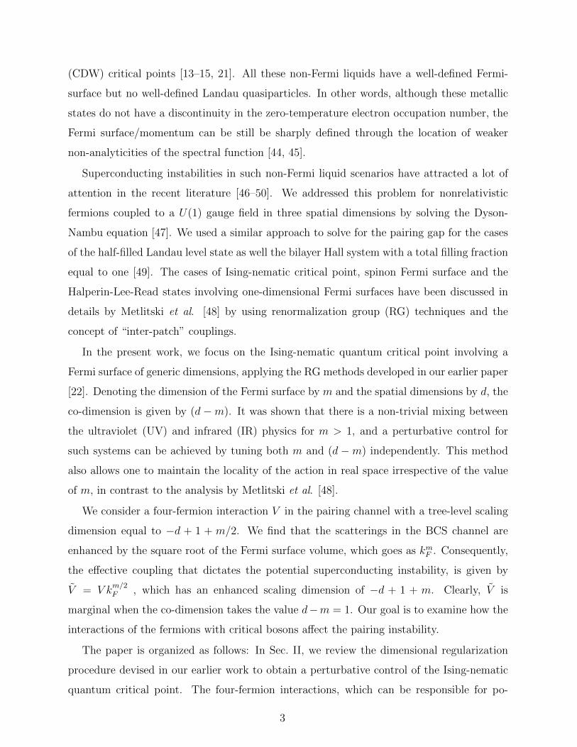
FIG. 1. Cartesian coordinates on a patch of an m-dimensional convex Fermi surface.

tential BCS instability, are introduced in Sec. III. There we compute the divergent terms

contributing to the beta-functions to the lowest order. The solutions to the RG equations

in various possible scenarios are discussed in Sec. III E. We conclude with a summary and

outlook in Sec. IV. The detailed computation of the relevant Feynman diagrams has been

shown in the appendix.

II. ISING-NEMATIC QUANTUM CRITICAL POINT

We consider the Ising-nematic quantum critical point involving an m-dimensional Fermi

surface interacting with a massless boson in d = (m+1) space dimensions [22], with coupling

constant e. The momentum of the critical boson is centered at zero. This system can be

described by the action

S =∑s=±,j

∫dk ψ†s,j(k)

[i k0 + s k1 + L2

(k))]ψs,j(k) +

1

2

∫dk[k2

0 + k21 + L2

(k)

]φ(−k)φ(k)

+e√N

∑s=±,j

∫dk dq φ(q) ψ†s,j(k + q)ψs,j(k) , (2.1)

written in a coordinate system centred at an arbitrary point K∗ of the convex Fermi

surface (see Fig. 1). Here, k is the (d + 1)-dimensional energy-momentum vector with

dk ≡ dd+1k(2π)d+1 . Assuming inversion symmetry, we have included the “right-moving” and “left-

moving” fermionic fields, ψ+,j and ψ−,j, representing K∗ and its antipodal point −K∗. These

4

fields represent fermions with flavours j = 1, 2, .., N , frequency k0 and momentum K∗α + kα

(−K∗α + kα) with 1 ≤ α ≤ d. k1 and L(k) ≡ (k2, k3, . . . , kd) denote the momentum compo-

nents perpendicular and parallel to the Fermi surface at ±K∗, respectively. The momenta

are rescaled such that the Fermi velocity, and the curvature of the Fermi surface at ±K∗,are equal to one.

A perturbative control of the Yukawa coupling (and the strength of UV/IR mixing in

non-Fermi liquid states with m > 1 [22]) is achieved by tuning the dimension [51–55] and

the co-dimension of the Fermi surface [20, 21, 56], i.e. by writing an action that describes

an m-dimensional Fermi surface embedded in the d-dimensional momentum space:

S =∑j

∫dk Ψj(k)

[iΓ ·K + i γd−m δk

]Ψj(k) exp

{L2(k)

µ kF

}+

1

2

∫dkL2

(k) φ(−k)φ(k)

+i e µx/2√

N

∑j

∫dk φ(q) Ψj(k + q) γd−mΨj(k) , (2.2)

where a mass scale µ is introduced to make kF and e dimensionless. Here

x = −d+ 2 +m

2, δk = kd−m + L2

(k) , kF = µ kF , ΨTj (k) =

(ψ+,j(k), ψ†−,j(−k)

). (2.3)

The gamma matrices associated with K have been written as Γ ≡ (γ0, γ1, . . . , γd−m−1). Since

in real systems, d−m lies between 1 and 2, we will consider only the 2×2 gamma matrices so

that the corresponding spinors always have two components. We will use the representation

where

Γ0 ≡ γ0 = σy , γd−m = σx (2.4)

are fixed in general dimensions. The bare fermion propagator is given by G0(k) =

1i

Γ·K+γd−mδkK2+δ2

kexp

{− L2

(k)

kF

}. Note that we have used an exponential factor in order to

damp out the fermion propagator, which acts as a soft cut-off for the directions tangential

to the Fermi surface in loop-integrals. This restricts the integration along the directions

tangent to the Fermi surface to a small region compared to kF by damping the propagation

of fermions with |L(k)| > k1/2F . We denote the UV cut-off for K and kd−m as Λ, which is nat-

urally given by the choice Λ = µ. Hence, two dimensionless parameters, e and kF = kF/Λ,

appear in the above action. If k is the typical energy at which we probe the system, we

must impose the restriction k << Λ << kF . The renormalization group flow is generated

by changing Λ and requiring that low-energy observables are independent of it.

5

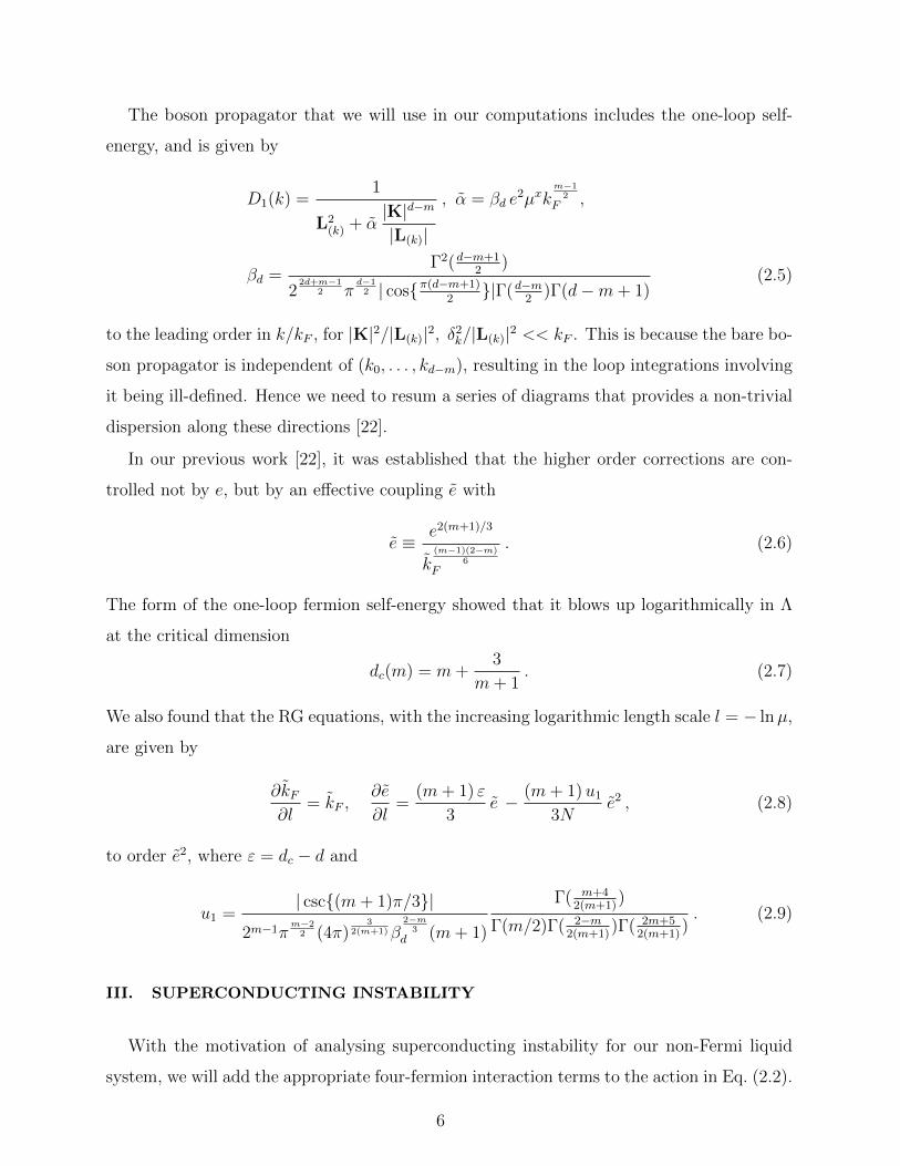
The boson propagator that we will use in our computations includes the one-loop self-

energy, and is given by

D1(k) =1

L2(k) + α

|K|d−m|L(k)|

, α = βd e2µxk

m−12

F ,

βd =Γ2(d−m+1

2)

22d+m−1

2 πd−1

2 | cos{π(d−m+1)2}|Γ(d−m

2)Γ(d−m+ 1)

(2.5)

to the leading order in k/kF , for |K|2/|L(k)|2, δ2k/|L(k)|2 << kF . This is because the bare bo-

son propagator is independent of (k0, . . . , kd−m), resulting in the loop integrations involving

it being ill-defined. Hence we need to resum a series of diagrams that provides a non-trivial

dispersion along these directions [22].

In our previous work [22], it was established that the higher order corrections are con-

trolled not by e, but by an effective coupling e with

e ≡ e2(m+1)/3

k(m−1)(2−m)

6F

. (2.6)

The form of the one-loop fermion self-energy showed that it blows up logarithmically in Λ

at the critical dimension

dc(m) = m+3

m+ 1. (2.7)

We also found that the RG equations, with the increasing logarithmic length scale l = − lnµ,

are given by

∂kF∂l

= kF ,∂e

∂l=

(m+ 1) ε

3e − (m+ 1)u1

3Ne2 , (2.8)

to order e2, where ε = dc − d and

u1 =| csc{(m+ 1)π/3}|

2m−1πm−2

2 (4π)3

2(m+1)β2−m

3d (m+ 1)

Γ( m+42(m+1)

)

Γ(m/2)Γ( 2−m2(m+1)

)Γ( 2m+52(m+1)

). (2.9)

III. SUPERCONDUCTING INSTABILITY

With the motivation of analysing superconducting instability for our non-Fermi liquid

system, we will add the appropriate four-fermion interaction terms to the action in Eq. (2.2).

6

We note that:∫ ( 4∏s=1

dps

)[{Ψj1(p3) Ψj2(p1)

}{Ψj3(p4) Ψj4(p2)

}−{

Ψj3(p3)σzΨj4(p1)}{

Ψj1(p4)σzΨj2(p2)}]

× F(p1, p3; p2, p4)

4

= −∫ ( 4∏

s=1

dps

)[ψ†+,j1(p3)ψ†−,j2(−p1)ψ−,j3(−p4)ψ+,j4(p2)

]F(p1, p3; p2, p4) ,

can give rise to BCS pairing, where F(p1, p3; p2, p4) is a function invariant under the simul-

taneous exchanges (p1, p3)↔ (p2, p4). Hence, we need to consider the four-fermion terms:

SSCgen =

µdv

4

∑j1,j2,j3,j4

∫ ( 4∏s=1

dps

)(2π)d+1 δ(d+1)(p1 + p2 − p3 − p4)

×[{Ψj1(p3)Ψj2(p1)} {Ψj3(p4)Ψj4(p2)} − {Ψj3(p3)σzΨj4(p1)} {Ψj1(p4)σzΨj2(p2)}

],

×[VS(p1,p3; p2,p4) (δj1,j3δj2,j4 − δj1,j4δj2,j3) + VA(p1,p3; p2,p4) (δj1,j3δj2,j4 + δj1,j4δj2,j3)

](3.1)

where k denotes the momentum components, (kd−m,L(k)), of the (d + 1)-dimensional

energy-momentum vector k. The subscript “S” (“A”) denotes that VS(p1,p3; p2,p4)

(VA(p1,p3; p2,p4)) is symmetric (antisymmetric) under the interchange p1 ↔ p3 or p2 ↔ p4.

Here we have have made the VS/A’s dimensionless by using the mass scale µ, with dv =

−d+ 1 + m2

representing the scaling dimension of VS/A.

We will find from our analysis of the RG flow, in order for superconducting instability to

set in, we must have p1 = p3 and p2 = p4. Furthermore, assumption of rotational symmetry

allows us to write:

VS/A(p1,p1; p2,p2) = VS/A(θ1 − θ2), (3.2)

where θ1,2 denote the angles for p1,2 on the Fermi surface. For simplicity and in order to

obtain analytic expressions, we will consider only the case of a constant non-zero VS , for

which we need at least two flavours of fermions. Then, with N = 2, Eq. (3.1) reduces to:

SSC = −µdvVS4

∑j1,j2

∫ ( 4∏s=1

dps

)(2π)d+1 δ(d+1)(p1 + p2 − p3 − p4) (1− δj1,j2)

×[{Ψj1(p3)Ψj2(p1)} {Ψj2(p4)Ψj1(p2)} − {Ψj1(p3)σzΨj2(p1)} {Ψj2(p4)σzΨj2(p1)}

],

(3.3)

7

VS VS

p1, j2

p3, j1 p4, j2

p2, j1

k, j1

p1 − p3 + k, j2

(a)

p4, j2p3, j1

p1, j2p2, j1

k, j1

k − p1 + p4, j1

VS

VS

(b)

p4, j2p3, j1

p1, j2 p2, j1

k, j2 p1 + p2 − k, j1

VS

VS

(c)

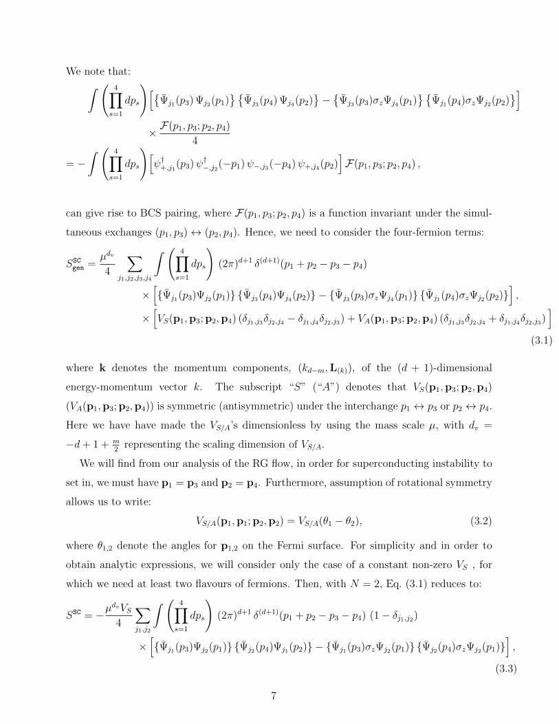
FIG. 2. One-loop diagrams proportional to V 2S . Here p4 = p1 + p2 − p3.

It is straightforward to apply our formalism for a system with a given number of flavours

and a specific angular dependence of VS/A.

A. One-loop diagrams generating terms proportional to V 2S

We need to consider one-loop diagrams as shown in Fig. 2 for contributions proportional to

V 2S . The computation of these diagrams has been detailed in Appendix A. The contribution

from Fig. 2a is found to be proportional to:

− (1− δj1,j2)2

∫dkTr

[G0(k + P1 −P3)G0(k)

]=

21−2d+m2 (1− δj1,j2) k

m/2F π1− d

2 sec(

(d−m)π2

)Γ(d−m

2

)|P3 −P1|−d+m+1

,

(3.4)

which is logarithmically divergent at d−m = 1 such that we can express it askm/2F ln

(Λ

|P1−P3|

)2

3m2 π1+m

2.

The results from Figs. 2b and 2c are kF -suppressed and hence do not contribute to the beta-

functions.

Noting that Tr[σz G0(k + P1 − P3)σz G0(k)

]= −Tr

[G0(k + P1 − P3)G0(k)

], the full

contribution from all one-loop diagrams proportional to V 2S is given by:

tV V =4× 2

2!

4

4× 4× 22+2d−m

2 km/2F µ2 dv V 2

S

πd2 Γ(d−m

2

)ε

+O (ε) =v2 µ

2 dv+m2 k

m/2F V 2

S

ε+O (ε) ,

v2 =22+2d−m

2

πd2 Γ(d−m

2

) , (3.5)

for d−m = 1− ε.

8

p1 , j2

p2 , j2 p1 , j1

p2 , j1

p1 − p2

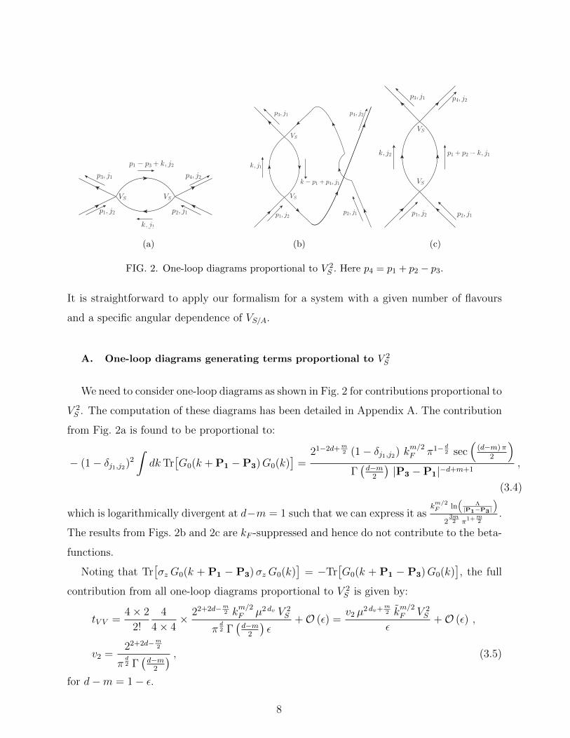
FIG. 3. Tree-level diagram proportional to e2.

B. UV-divergent terms proportional to e

Following earlier studies [46, 48], we have to include contributions from tree-level BCS

channel, which are generated from long-range interactions between the fermions. In this

case, the long-range interaction is mediated by the massless boson. Here we treat this

contribution in the language of dimensional regularization as we have done for the other

terms. In Appendix C, we have provided an alternative treatment of these terms in the

more familiar Wilsonian RG language.

We consider Fig. 3, which gives the terms∑j1,j2

[− ψ†+,j1(p2)ψ†−,j2(−p2)ψ−,j2(−p1)ψ+,j1(p1)− ψ†+,j1(p1)ψ†−,j2(−p1)ψ−,j2(−p2)ψ+,j1(p2)

−ψ†+,j1(p2)ψ+,j1(p1)ψ†+,j2(p1)ψ+,j2(p2)− ψ†−,j2(−p2)ψ−,j2(−p1)ψ†−,j1(−p1)ψ−,j1(−p2)]

multiplying (ie)2µxD1(p1−p2)2N

. Due to symmetry of D1(p1− p2) under p1 ↔ p2, they contribute

as e2µxD1(p1−p2)N

for terms responsible for BCS instability.

Using L2(q) ' 2 k2

F (1 − cos θ)/kF ⇒ |L(q)| '√kF |θ|, the decomposition into angular

momentum channels for an m-dimensional Fermi surface leads to the contribution being

proportional to:

tee 'e2 Λx

2N× 2

∫θ>0

dθθm−1 |L(q)|

L3(q) + α |Q|d−m =

e2 Λx

N km/2F

∫θ>0

d|L(q)||L(q)|m

L3(q) + α |Q|d−m

=e2 Λx Γ

(m+1

3

)Γ(

2−m3

)3N k

m/2F α

2−m3 |Q| (d−m)(2−m)

3

, (3.6)

which is independent of the angular momentum channel. This expression tells us that for

m = 2− δ and d = m+ 1− γ ε, we get a pole such that tee 'eΛ

γ ε+(2−m) (m−1)

6 (m+1) Γ(m+13 )

β2−m

3d N k

m/2F

1δ, which

is equivalent to the logarithmically divergent terme2 Λx Γ(m+1

3 )N k

m/2F

ln

(√kF

α13 |Q|

d−m3

). This term,

9

k VS

p1, j2 p2, j1p1 − k, j2

p3 − k, j1 p4, j2p3, j1

(a)

kVS

p1, j2 p2, j1

p4 − k, j2

p2 − k, j1

p4, j2p3, j1

(b)

k − p3

p1, j2 p2, j1

p3, j1 p4, j2

k, j1 p1 + p2 − k, j2

VS

(c)

p1 − kp1, j2 p2, j1

p3, j1 p4, j2

k, j2 p1 + p2 − k, j1VS

(d)

VS

p1, j2 p2, j1p1 − k, j2

p4, j2p3, j1

k

p4 − k, j2

(e)

VS

p1, j2 p2, j1p2 − k, j1

p4, j2p3, j1

kp3 − k, j1

(f)

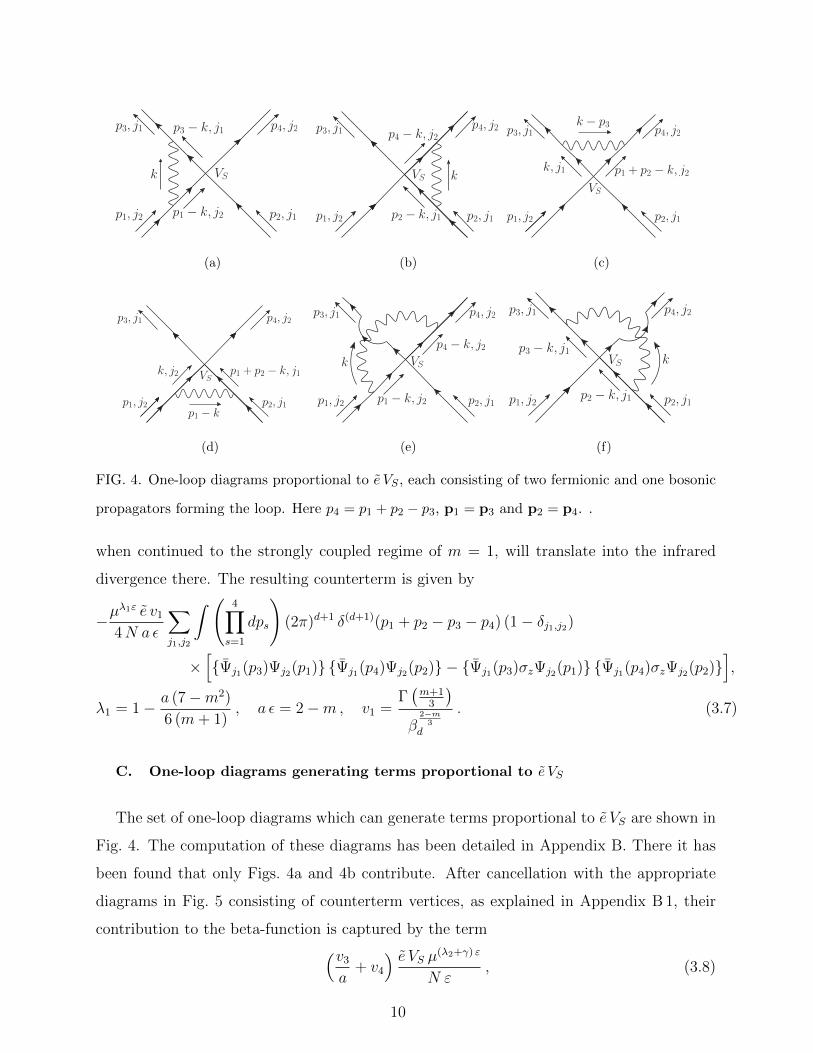
FIG. 4. One-loop diagrams proportional to e VS , each consisting of two fermionic and one bosonic

propagators forming the loop. Here p4 = p1 + p2 − p3, p1 = p3 and p2 = p4. .

when continued to the strongly coupled regime of m = 1, will translate into the infrared

divergence there. The resulting counterterm is given by

−µλ1ε e v1

4N a ε

∑j1,j2

∫ ( 4∏s=1

dps

)(2π)d+1 δ(d+1)(p1 + p2 − p3 − p4) (1− δj1,j2)

×[{Ψj1(p3)Ψj2(p1)} {Ψj1(p4)Ψj2(p2)} − {Ψj1(p3)σzΨj2(p1)} {Ψj1(p4)σzΨj2(p2)}

],

λ1 = 1− a (7−m2)

6 (m+ 1), a ε = 2−m, v1 =

Γ(m+1

3

)β

2−m3

d

. (3.7)

C. One-loop diagrams generating terms proportional to e VS

The set of one-loop diagrams which can generate terms proportional to e VS are shown in

Fig. 4. The computation of these diagrams has been detailed in Appendix B. There it has

been found that only Figs. 4a and 4b contribute. After cancellation with the appropriate

diagrams in Fig. 5 consisting of counterterm vertices, as explained in Appendix B 1, their

contribution to the beta-function is captured by the term(v3

a+ v4

) e VS µ(λ2+γ) ε

N ε, (3.8)

10

e VS

p1, j2

p3, j1 p4, j2

p2, j1

k, j1

p1 − p3 + k, j2

(a)

VS e

p1, j2

p3, j1 p4, j2

p2, j1

k, j1

p1 − p3 + k, j2

(b)

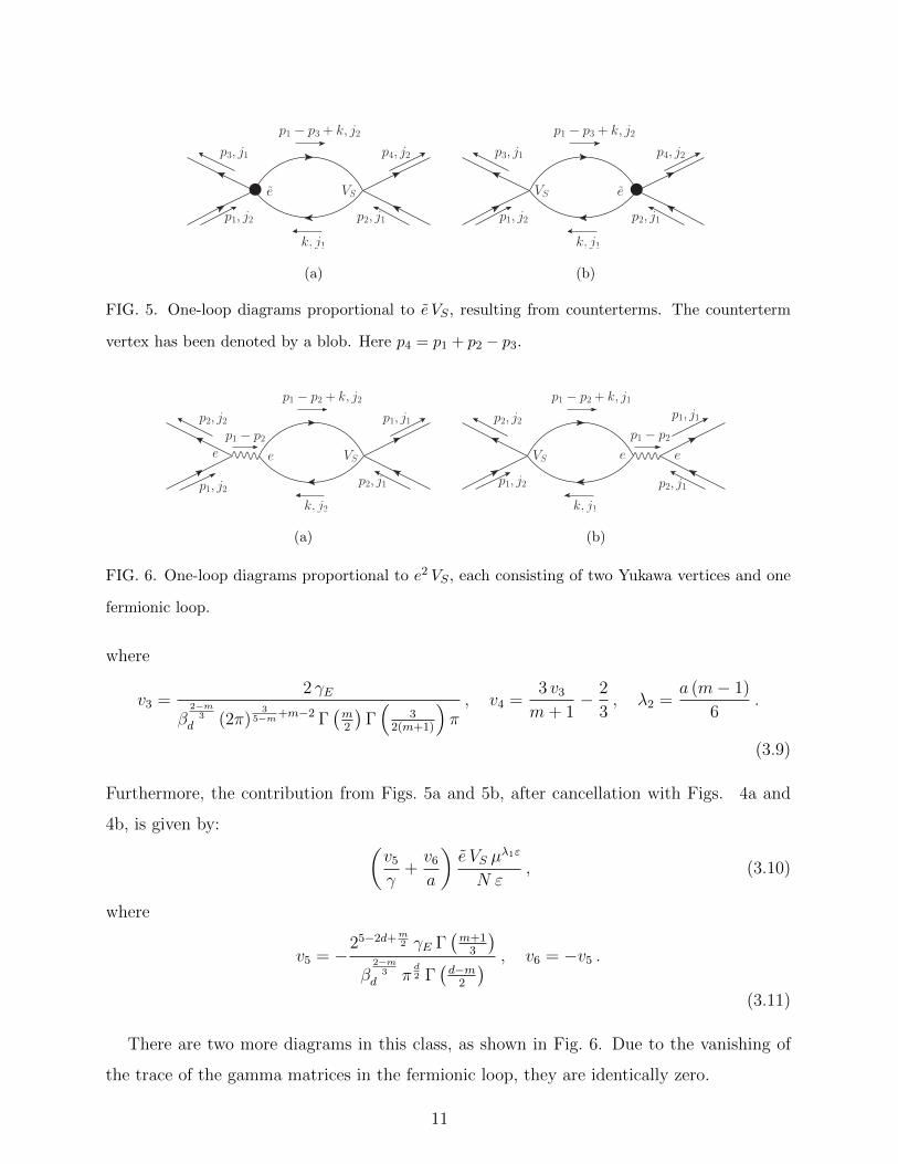
FIG. 5. One-loop diagrams proportional to e VS , resulting from counterterms. The counterterm

vertex has been denoted by a blob. Here p4 = p1 + p2 − p3.

e VS

p1, j2

p2, j2 p1, j1

p2, j1

k, j2

p1 − p2 + k, j2

e

p1 − p2

(a)

VS e

p1, j2

p2, j2 p1, j1

p2, j1

k, j1

p1 − p2 + k, j1

e

p1 − p2

(b)

FIG. 6. One-loop diagrams proportional to e2 VS , each consisting of two Yukawa vertices and one

fermionic loop.

where

v3 =2 γE

β2−m

3d (2π)

35−m+m−2 Γ

(m2

)Γ(

32(m+1)

)π, v4 =

3 v3

m+ 1− 2

3, λ2 =

a (m− 1)

6.

(3.9)

Furthermore, the contribution from Figs. 5a and 5b, after cancellation with Figs. 4a and

4b, is given by: (v5

γ+v6

a

)e VS µ

λ1ε

N ε, (3.10)

where

v5 = −25−2d+m2 γE Γ

(m+1

3

)β

2−m3

d πd2 Γ(d−m

2

) , v6 = −v5 .

(3.11)

There are two more diagrams in this class, as shown in Fig. 6. Due to the vanishing of

the trace of the gamma matrices in the fermionic loop, they are identically zero.

11

D. Beta-functions for the coupling constants

We have found that the one-loop divergent terms are proportional tokm2F µ2dv

γ εV 2S for d −

m = 1 − γ ε , for |γ ε| � 1. Hence, the upper critical dimension for the four-fermion BCS

interaction is dc = m+1, which is different from dc = m+ 3m+1

for the Yukawa coupling (see

Eq. (2.7)). For m = 2, dc = dc = 3. However, for m = 1, dc = 5/2 and dc = 2. In order to

study both the physically relevant cases of m = 1 and m = 2, we define γ and ε such that

dc − ε = dc − γ ε ⇒ γ ε = ε− 2−mm+ 1

. (3.12)

Furthermore, from the form of the divergent terms, it is apparent that

VS = km/2F VS (3.13)

is the effective coupling constant for the four-fermion interactions, which has an enhanced

tree-level scaling dimension given by dv+1/2 = dc−d. VS is marginal when the co-dimension

d−m = 1.

The counterterms for the four-fermion interaction term take the form:

SSCct = −µ

γ εASVS4

∑j1,j2

∫ ( 4∏s=1

dps

)(2π)d+1 δ(d+1)(p1 + p2 − p3 − p4) (1− δj1,j2)

×[{Ψj1(p3)Ψj2(p1)} {Ψj1(p4)Ψj2(p2)} − {Ψj1(p3)σzΨj2(p1)} {Ψj1(p4)σzΨj2(p2)}

],

(3.14)

where we use the definition

AS ≡ ZS − 1 =∞∑

α1=1

ZS,α1(e, kF , VS)

εα1. (3.15)

Adding the counterterms to the original SSC, and denoting the bare quantities by the super-

script “B”, we obtain the renormalized four-fermion interaction as:

SSCren = −V

BS

4

∑j1,j2

∫ ( 4∏s=1

dpBs

)(2π)d+1 δ(d+1)(pB1 + pB2 − pB3 − pB4) (1− δj1,j2)

×[{ΨB

j1(p3)ΨB

j2(p1)} {ΨB

j1(p4)ΨB

j2(p2)} − {ΨB

j1(p3)σzΨ

Bj2

(p1)} {ΨBj1

(p4)σzΨBj2

(p2)}],

(3.16)

where

K =Z2

Z1

KB , kd−m = kB,d−m , L(k) = L(k),B , Ψ(k) = Z−1/2Ψ ΨB(kB) , φ(k) = Z

−1/2φ φB(kB) ,

eB = Z−1/23

(Z2

Z1

)(d−m)/2

µx/2 e , kF = µ kF , V BS k

m/2F = ZS Z

−2ψ

(Z2

Z1

)3(d−m)

µγ ε VS . (3.17)

12

The dynamical critical exponent and the anomalous dimension for the fermions are given

by [22]:

z = 1 +m+ 1

3Nu1 e, ηψ = (1− z)(d−m)/2 , (3.18)

with u1 defined in Eq. (2.9). Using the definition 2−m = a ε⇒ a = 3 (1−γ)1 + (1−γ) ε

, we have

ZS,1 VS µγ ε

ε=

(v1

a+ v5VS

γ+ v6VS

a

)e µλ1 ε

N ε+v2 V

2S µ

γ ε

γ ε+

(v3

a+ v4

)e VS µ

(λ2+γ)ε

N ε. (3.19)

Implementing the condition dd lnµ

(V BS k

m/2F

)= 0, we get

βV +

{v1

a+(v3+v6

a+ v4 + v5

γ

)VS

}βe +

(v3+v6

a+ v4 + v5

γ

)βV e

N ε+

2 v2 VS βVγ ε

+{γ ε− 4 ηψ + 3 (d−m) (1− z)

}(VS +

v2 V2S

γ ε

)

+{λ1 ε− 4 ηψ + 3 (d−m) (1− z)

}(v1

a+ v5VS

γ+ v6VS

a

)e

N ε

+{

(λ2 + γ) ε− 4 ηψ + 3 (d−m) (1− z)}(v3

a+ v4

)e VS

N ε= 0 ,

where βV ≡∂VS∂ lnµ

= β(0)V + β

(1)V ε, βe ≡

∂e

∂ lnµ= −m+ 1

3ε e+O

(e2). (3.20)

Comparing the coefficients of the different powers of ε on both sides, the solution takes the

form:

∂VS∂l

= γ εVS − v2V2S −

(7−m2) v1

6N (m+ 1)e

+[(5−m2 − 2m) (3 v5 − v6)

m+ 1+ (m− 1) v3 − 2 (m+ 1) (u1 + v4)

] e VS6N

, (3.21)

upto O (e2, e ε, ε2) in one-loop corrections. This can be simplified as:

∂VS∂l

=

(ε− 1

2

)VS − v2V

2S − v1

2Ne+ 3 v5−4 v4−v6−4u1

6Ne VS for m = 1 ,

γ εVS − v2V2S − v1

6Ne+ v3+6 v4−3 v5+v6−6u1

6Ne VS for m = 2 and γ = ±1 .

(3.22)

E. Fixed points of the beta functions

The fixed points for the beta functions can be found from the solutions of ∂VS∂l

= 0 and

∂e∂l

= 0, using Eqs. (2.8) and (3.22). The quadratic equation for the fixed point values of

13

(a) (b)

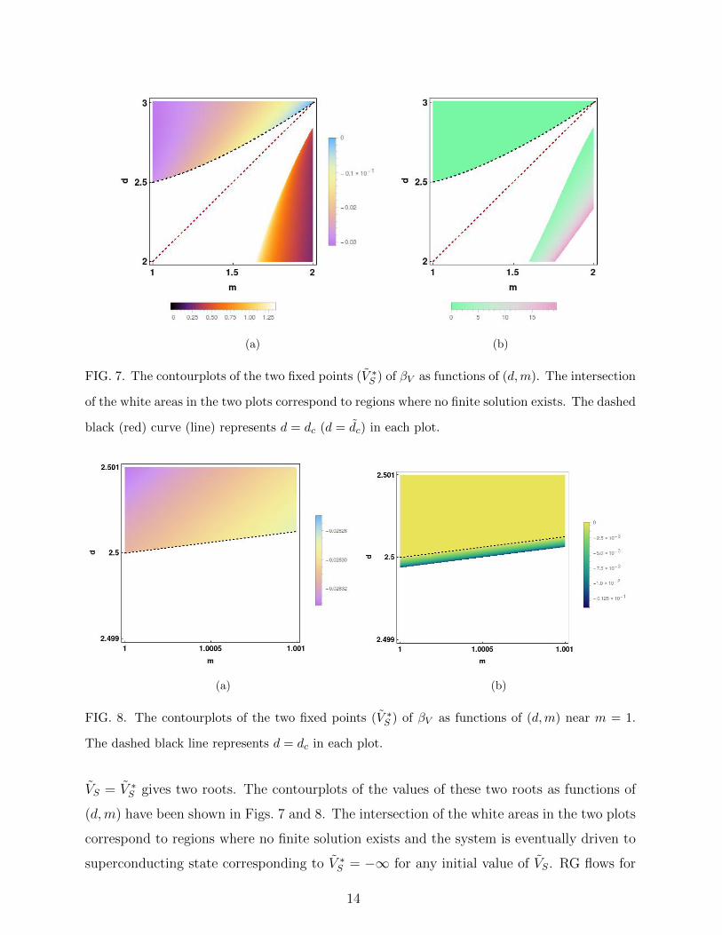
FIG. 7. The contourplots of the two fixed points (V ∗S ) of βV as functions of (d,m). The intersection

of the white areas in the two plots correspond to regions where no finite solution exists. The dashed

black (red) curve (line) represents d = dc (d = dc) in each plot.

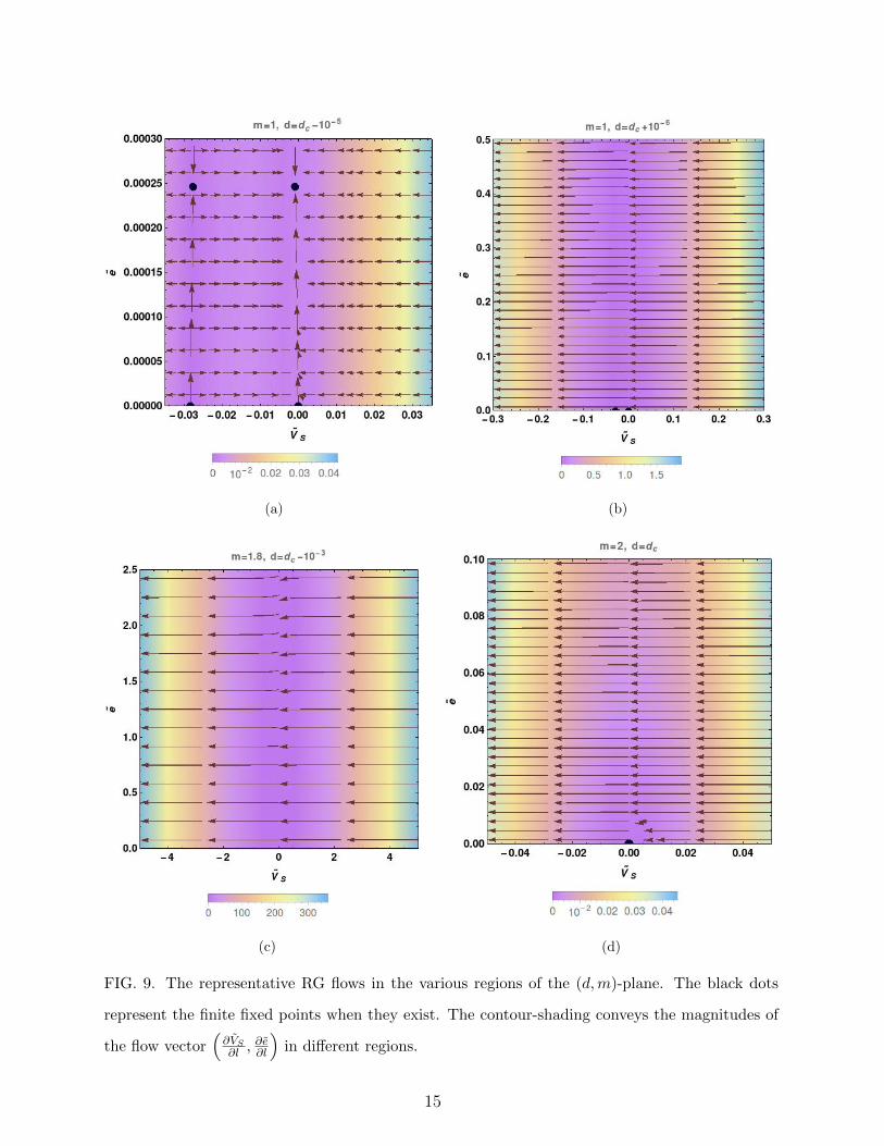
(a) (b)

FIG. 8. The contourplots of the two fixed points (V ∗S ) of βV as functions of (d,m) near m = 1.

The dashed black line represents d = dc in each plot.

VS = V ∗S gives two roots. The contourplots of the values of these two roots as functions of

(d,m) have been shown in Figs. 7 and 8. The intersection of the white areas in the two plots

correspond to regions where no finite solution exists and the system is eventually driven to

superconducting state corresponding to V ∗S = −∞ for any initial value of VS. RG flows for

14

(a) (b)

(c) (d)

FIG. 9. The representative RG flows in the various regions of the (d,m)-plane. The black dots

represent the finite fixed points when they exist. The contour-shading conveys the magnitudes of

the flow vector(∂VS∂l ,

∂e∂l

)in different regions.

15

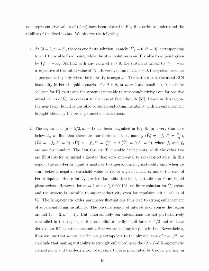
some representative values of (d,m) have been plotted in Fig. 9 in order to understand the

stability of the fixed points. We observe the following:

1. At (d = 3,m = 2), there is one finite solution, namely (V ∗S = 0, e∗ = 0), corresponding

to an IR unstable fixed point, while the other solution is an IR stable fixed point given

by V ∗S = −∞. Starting with any value of e > 0, the system is driven to VS = −∞irrespective of the initial value of VS. However, for an initial e = 0, the system becomes

superconducting only when the initial VS is negative. The latter case is the usual BCS

instability in Fermi liquid scenario. For d < dc at m = 2 and small ε > 0, no finite

solution for V ∗S exists and the system is unstable to superconductivity even for positive

initial values of VS, in contrast to the case of Fermi liquids [57]. Hence in this region,

the non-Fermi liquid is unstable to superconducting instability with an enhancement

brought about by the order parameter fluctuations.

2. The region near (d = 5/2,m = 1) has been magnified in Fig. 8. In a very thin slice

below dc, we find that there are four finite solutions, namely (V ∗S = −f1, e∗ = N ε

u1),

(V ∗S = −f2, e∗ = 0), (V ∗S > −f1, e

∗ = N εu1

) and (V ∗S = 0, e∗ = 0), where f1 and f2

are positive number. The first two are IR unstable fixed points, while the other two

are IR stable for an initial e greater than zero and equal to zero respectively. In this

region, the non-Fermi liquid is unstable to superconducting instability only when we

start below a negative threshold value of VS for a given initial e, unlike the case of

Fermi liquids. Hence for VS greater than this threshold, a stable non-Fermi liquid

phase exists. However, for m = 1 and ε & 0.000123, no finite solution for V ∗S exists

and the system is unstable to superconductivity even for repulsive initial values of

VS. The Ising-nematic order parameter fluctuations thus lead to strong enhancement

of superconducting instability. The physical region of interest is of course the region

around (d = 2,m = 1). But unfortunately our calculations are not perturbatively

controlled in this region, as e is not infinitesimally small for ε ∼ 1/2 and we have

derived our RG equations assuming that we are looking for poles in 1/ε. Nevertheless,

if we assume that we can continuously extrapolate to the physical case of ε = 1/2, we

conclude that pairing instability is strongly enhanced near the (2 + 1)-d Ising-nematic

critical point and the destruction of quasiparticles is preempted by Cooper pairing, in

16

agreement with Ref. [48].

A few comments are in order regarding the enhanced superconducivity near (d = 3,m =

2) and (d = 2,m = 1). The Yukawa-like coupling e gives rise to an effective attractive

interaction for Cooper pairing and hence drives the system towards superconductivity even

with an initially positive value of VS, as long as e is non-zero, as the flow continues towards

the IR stable fixed point at V ∗S = −∞. It can be shown that the energy scale at which this

happens is always larger than the non-Fermi liquid energy scale (ı.e. the scale where the

non-Fermi liquid effects become appreciable). However, the magnitude of the pairing gap

will depend on the initial values of the coupling constants. An analysis along these lines is

very similar to that of Metlitski et al. [48] and their estimate regarding the pairing gap holds

after taking appropriate values of ε, namely ε ' 0 and ε = 1/2 for solving the (d = 3,m = 2)

and (d = 2,m = 1) cases respectively.

IV. SUMMARY AND OUTLOOK

We have used RG to study potential superconducting instability induced by four-fermion

interactions for Ising-nematic quantum critical points, in a perturbative expansion near the

upper critical dimension dc(m) of the order parameter coupling with quasiparticles. Using

the small parameter ε = dc(m) − d, the RG flow equations and fixed points for both the

effective order parameter coupling e and BCS-channel coupling VS have been computed as

functions of d and m. We have found that for (d = 3,m = 2), the flow towards the non-

Fermi liquid fixed point is preempted by Cooper pairing, such that for an initial e > 0,

an attractive or repulsive four-fermion interaction in the BCS-channel eventually leads to

superconductivity, enhanced by the coupling e. In a thin slice near (d = 5/2,m = 1) such

that 0 < ε . 10−4, the non-Fermi liquid fixed point is stable for Vs larger than a negative

threshold value. To reach the physical scenario with (d = 2,m = 1), we have to set ε = 1/2,

which is not quite perturbatively controlled. However, if we extrapolate our results for

ε > 10−4 to d = 2, then the (2 + 1)-d quantum critical point is expected to have strong

enhancement of superconductivity by the order parameter fluctuations, such that even an

17

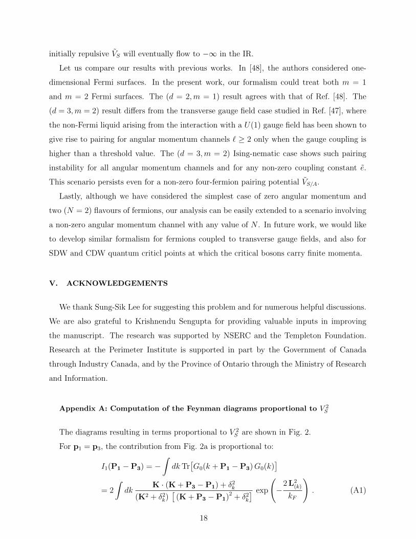
initially repulsive VS will eventually flow to −∞ in the IR.

Let us compare our results with previous works. In [48], the authors considered one-

dimensional Fermi surfaces. In the present work, our formalism could treat both m = 1

and m = 2 Fermi surfaces. The (d = 2,m = 1) result agrees with that of Ref. [48]. The

(d = 3,m = 2) result differs from the transverse gauge field case studied in Ref. [47], where

the non-Fermi liquid arising from the interaction with a U(1) gauge field has been shown to

give rise to pairing for angular momentum channels ` ≥ 2 only when the gauge coupling is

higher than a threshold value. The (d = 3,m = 2) Ising-nematic case shows such pairing

instability for all angular momentum channels and for any non-zero coupling constant e.

This scenario persists even for a non-zero four-fermion pairing potential VS/A.

Lastly, although we have considered the simplest case of zero angular momentum and

two (N = 2) flavours of fermions, our analysis can be easily extended to a scenario involving

a non-zero angular momentum channel with any value of N . In future work, we would like

to develop similar formalism for fermions coupled to transverse gauge fields, and also for

SDW and CDW quantum criticl points at which the critical bosons carry finite momenta.

V. ACKNOWLEDGEMENTS

We thank Sung-Sik Lee for suggesting this problem and for numerous helpful discussions.

We are also grateful to Krishnendu Sengupta for providing valuable inputs in improving

the manuscript. The research was supported by NSERC and the Templeton Foundation.

Research at the Perimeter Institute is supported in part by the Government of Canada

through Industry Canada, and by the Province of Ontario through the Ministry of Research

and Information.

Appendix A: Computation of the Feynman diagrams proportional to V 2S

The diagrams resulting in terms proportional to V 2S are shown in Fig. 2.

For p1 = p3, the contribution from Fig. 2a is proportional to:

I1(P1 −P3) = −∫dkTr

[G0(k + P1 −P3)G0(k)

]= 2

∫dk

K · (K + P3 −P1) + δ2k

(K2 + δ2k)[

(K + P3 −P1)2 + δ2k

] exp

(−

2 L2(k)

kF

). (A1)

18

Shifting the dummy variable kd−m → kd−m + L2(k) and using Feynman parametrization, we

obtain:

I1(P1 −P3) = 2

∫dk

∫ 1

0

dtK · (K + P3 −P1) + k2

d−m[(1− t)

(K2 + k2

d−m)

+ t (K + P3 −P1)2 + t k2d−m

]2 exp

(−

2 L2(k)

kF

)

= 2

∫dk

∫ 1

0

dtK2 − t (1− t) (P3 −P1)2 + k2

d−m[K2 + k2

d−m + t (1− t) (P3 −P1)2 ]2 exp

(−

2 L2(k)

kF

). (A2)

In the last line, we have performed the variable shift K→ K− t (P3 −P1). The remaining

integrals can be computed in a straightforward manner to give:

I1(P1 −P3) =21−2d+m

2 km/2F π1− d

2 sec(

(d−m)π2

)|P3 −P1|d−m−1

Γ(d−m

2

) , (A3)

which is logarithmically divergent at d−m = 1.

However, for p1 6= p3, the contribution from Fig. 2a is proportional to:

I1(p1 − p3) = −∫dkTr

[G0(k + p1 − p3)G0(k)

]= −βd

|P1 −P3|d−m km−1

2F

|L(p1−p3)|(A4)

where βd is defined in Eq. (2.5). This integral is the same as appears in the computation

of the one-loop self-energy Π(q) for the bosonic propagator [22], and is convergent. So we

must have p1 = p3 to get a contribution to the RG equations.

For Fig. 2b, the contribution is proportional to:

I2(p2 − p3) = −∫dkTr

[G0(k + p2 − p3)G0(k)

]=

I1(P2 −P3) for |L(p2−p3)| � |P2−P3|√kF

,

I1(p2 − p3) for |L(p2−p3)| � |P2−P3|√kF

.

Performing the angular momentum decomposition, we get∫dθ θm−1I2(p2 − p3)

=

∫ |P2−P3|√kF

0

d|L(p2−p3)||L(p2−p3)|m−1I2(p2 − p3)

km2F

+

∫ ∞|P2−P3|√

kF

d|L(p2−p3)||L(p2−p3)|m−1I2(p2 − p3)

km2F

={21−2d+m

2 π1− d2 sec

((d−m)π

2

)mΓ

(d−m

2

)km2F

+βd

m− 1

} |P2 −P3|d−1

km2F

, (A5)

which is suppressed by 1/kmF compared to the terms contributing to the beta functions.

19

In Fig. 2c, using the notation q2 ≡ p1 + p2, we find that near d − m = 1, the terms

resulting from the loop integral can be simplified and are proportional to

∫ ( 4∏s=1

dps

)δ(d+1)(p1 + p2 − p3 − p4)× 1− δj1,j2

(K2 + δ2k)[

(K−Q2)2 + δ2k−q2

]×∑j1,j2

∫dd−mK

[ {Ψj2(p3) γ0 Ψj2(p2)

}{Ψj1(p4) γ0 Ψj1(p1)

}K · (Q2 −K)

+{

Ψj2(p3) γd−m Ψj2(p2)}{

Ψj1(p4) γd−m Ψj1(p1)}δk δk−q2

]+ terms not contributing to Cooper pairing

= 2

∫ ( 4∏s=1

dps

)δ(d+1)(p1 + p2 − p3 − p4)

∑j1,j2

ψ†+,j2(p3)ψ†−,j1(−p1)ψ−,j1(−p4)ψ+,j2(−p3) (1− δj1,j2)

× I3(q2) + terms not contributing to Cooper pairing ,

where

I3(q2) =

∫dd−mK

K · (Q2 −K) + δk δk−q2

(K2 + δ2k)[

(K−Q2)2 + δ2k−q2

] exp

(−

2 L2(k)

kF

)= I2(q2) ,

(A6)

which therefore do not contribute to the RG-flow.

Appendix B: One-loop diagrams proportional to e VS

The first set of diagrams generating terms proportional to e2 VS is shown in Fig. 4. We

will use M to denote the matrices belonging to the set {σz, I2×2}.The term arising from Fig. 4a is given by:

t1M(p1, p2, p3)

= −VS (ie)2 µx+dv

4N(1− δj1,j2)× 2

2!

×∫dk D1(k){Ψj1(p3)Mγd−mG0(p3 − k)G0(p1 − k)γd−mΨj2(p1)}{Ψj2(p4)MΨj1(p2)}

= −VS e2 µx+dv (1− δj1,j2)

4N{Ψj1(p3)MΨj2(p1)} {Ψj2(p4)MΨj1(p2)} J1 , (B1)

20

where

J1 = i2∫dk γd−mG0(p3 − k)G0(p1 − k) γd−mD1(k)

=

∫dk

(K + P1) · (K + P3) + δ2k+p1

{(K + P1)2 + δ2k+p1} {(K + P3)2 + δ2

k+p1}[L2

(k) + α |K|d−m

|L(k)|

] .(B2)

Shifting kd−m → (k − p1)d−m − L2(k+p1), K→ K−P3, and performing the L(k)-integral, we

get

J1 =| csc{ (m+1)π

3}| πm

2

3 Γ(m2

)α

2−m3

∫dd−mK dkd−m

(2π)dK · (K + Q3) + k2

d−m

{(K + Q)2 + k2d−m} {K2 + k2

d−m} |K−P3|2β

' | csc(δπ3

)|πm

2

3 Γ(m2

)αδ3

∫ 1

0

dt

∫dd−mK dkd−m(2π)d |K|2β

K · (K + Q3) + k2d−m

{t (K + Q3)2 + (1− t) K2 + k2d−m}2

[1 +

δ (d− 2 + δ) K ·P3

3 K2

]=| csc

(δπ3

)|π1+m

2

6 Γ(m2

)αδ3

∫ 1

0

dt

∫dd−mK

(2π)d |K|2βK · (K + Q3) + t (K + Q3)2 + (1− t) K2

{t (K + Q3)2 + (1− t) K2} 32

×[1 +

δ (d− 2 + δ) K ·P3

3 K2

], (B3)

where

Q3 = P1 −P3, β =(d−m) (2−m)

6, m = 2− δ, d = m+

3

m+ 1− ε . (B4)

such that ε = ε(1− δ

3

). We have expanded the expression in terms of small P3, which

enables us to analyse the singularity structure without any loss of generality. Defining

D = K2 + t (1− y) (1− t + y t) Q23, we get

J1 =| csc

(δπ3

)|π1+m

2 Γ(β + 3

2

)6 Γ(m2

)αδ3 Γ(β) Γ

(32

) ∫ 1

0

dy

∫ 1

0

dt

∫dd−mK

(2π)d2K2 + y t (1− 2 t+ 2 y t) Q2

3

Dβ+ 32

yβ−1√

1− y

×[1− (2 β + 3) t2 (1− y) Q3 ·P3

D]

=| csc

(δπ3

)|

6 αδ3 (2π)

33+δ−δ Γ

(1− δ

2

)Γ(

36−2 δ

) 1

ε(1− δ

3

)|Q3|ε(1− δ

3)+O(1) .

(B5)

This is logarithmically divergent at d = dc. Near (d = 3,m = 2), we expand in small delta

such that

J1 =1

4 π2

1

δ ε(1− δ

3

)|Q3|ε(1− δ

3)+O(1) . (B6)

21

This indicates there is a log2 divergence. We note that there is no P3-dependent term

divergent in 1δ

or 1

ε(1− δ3)

. In fact, the leading order term dependent on P3 goes as

1−2 ln 24π5

Q3·P3

|Q3|2+ε(1− δ3)

.

The term arising from Fig. 4b has a divergent structure identical to Fig. 4a. Depending

on m, these two diagrams are of either higher order than or same order as the V 2S terms.

Near (d = 5/2,m = 1), these have only a pole in ε (and not in δ) and hence are of leading

order. On the other hand, near (d = 3,m = 2), these have two poles (one in ε and one

in δ) and hence are one order higher than the V 2S terms. In this second scenario, namely

near (d = 3,m = 2), these two diagrams must then be considered in conjunction with

those consisting of the counterterm vertices generated from the divergence of the angular

momentum decomposition of Fig. 3, as shown in Fig. 5. In Sec. B 1, we have shown how

these terms cancel out around this region.

The term arising from Fig. 4c is given by:

t3M(p1, p2, p3)

= −VS (ie)2 µx+dv

4N(1− δj1,j2)

×∫dk D1(k − p3){Ψj1(p3)γd−mG0(k)MΨj2(p1)}{Ψj2(p4)γd−mG0(p1 + p2 − k)MΨj1(p2)}

' −VS e2 µx+dv

4N(1− δj1,j2) {Ψj1(p3)MΨj2(p1)} {Ψj2(p4)MΨj1(p2)} J3 , (B7)

where we have dropped terms irrelevant for superconductivity such that

J3 = −∫dk

K · (K−P1 −P2)− δk δk−p1−p2

{K2 + δ2k} {(K−P1 −P2)2 + δ2

k−p1−p2}[L2

(k−p3) + α |K−P3|d−m|L(k−p3)|

] = 0 , (B8)

on performing the kd−m integral. Similarly, the contribution from Fig. 4d also vanishes.

Next we consider Fig. 4e, again only keeping terms relevant for superconductivity. This

contributes as:

t5M(p1, p2, p3)

= −VS (ie)2 µx+dv

4N(1− δj1,j2)

×∫dk D1(k){Ψj1(p3)MG0(p1 − k)γd−mΨj2(p1)}{Ψj2(p4)γd−mG0(p4 − k)MΨj1(p2)}

' −VS e2 µx+dv

4N(1− δj1,j2) {Ψj1(p3)MΨj2(p1)} {Ψj2(p4)MΨj1(p2)} J5 , (B9)

22

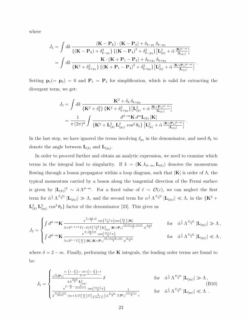
where

J5 =

∫dk

(K−P1) · (K−P4) + δk−p1 δk−p4

{(K−P1) + δ2k−p1} {(K−P4)2 + δ2

k−p4}[L2

(k) + α |K|d−m

|L(k)|

]=

∫dk

K · (K + P1 −P4) + δk+p1 δk+p2

{K2 + δ2k+p1} {(K + P1 −P4)2 + δ2

k+p2}[L2

(k) + α |K+P1|d−m|L(k)|

] .Setting p1(= p3) = 0 and P1 = P4 for simplification, which is valid for extracting the

divergent term, we get:

J5 =

∫dk

K2 + δk δk+p2

{K2 + δ2k} {K2 + δ2

k+p2}[L2

(k) + α |K+P1|d−m|L(k)|

]=

1

π (2π)d

∫dd−mK dmL(k) |K|

{K2 + L2(k) L2

(p2) cos2 θk}[L2

(k) + α |K+P1|d−m|L(k)|

] .In the last step, we have ignored the terms involving δp2 in the denominator, and used θk to

denote the angle between L(k) and L(p2).

In order to proceed further and obtain an analytic expression, we need to examine which

terms in the integral lead to singularity. If k = (K, kd−m,L(k)) denotes the momentum

flowing through a boson propagator within a loop diagram, such that |K| is order of Λ, the

typical momentum carried by a boson along the tangential direction of the Fermi surface

is given by |L(k)|3 ∼ αΛd−m. For a fixed value of e ∼ O(ε), we can neglect the first

term for α13 Λ

d−m3 |L(p2)| � Λ, and the second term for α

13 Λ

d−m3 |L(p2)| � Λ, in the {K2 +

L2(k) L2

(p2) cos2 θk} factor of the denominator [23]. This gives us

J5 =

∫dd−mK

π7−2d−δ

2 csc( δ−13π) sec( δπ2 ) |K|

3×2d−1+δ Γ(−δ) Γ( 1+δ2 )L2

(p2)|K+P1|

(2+δ) (d−2+δ)3 α

2+δ3

for α13 Λ

d−m3 |L(p2)| � Λ ,

∫dd−mK

π4−2d+m

2 csc(m+13π)

3×2d−1 Γ(m2 ) |K| |K+P1|(d−m) (2−m)

3 α2−m

3

for α13 Λ

d−m3 |L(p2)| � Λ ,

where δ = 2−m. Finally, performing the K integrals, the leading order terms are found to

be:

J5 =

√

3 |P1|4−(1− δ3) ε−2δ+(1− δ3) ε δ

3−δ

4 α2+δ

3 L2(p2)

δ for α13 Λ

d−m3 |L(p2)| � Λ ,

π2−m2 −

32 (m+1) csc(m+1

3π)

2m (2−m)m+1 (m+1) Γ(m2 ) Γ( 3

2 (m+1)) α2−m

3

1

2 |P1|(m+1) ε

3 εfor α

13 Λ

d−m3 |L(p2)| � Λ .

(B10)

23

Now we need to carry out the angular momentum decomposition to get

e2

∫dθ θm−1J5 = e2

∫ Λ3−d+m

3

α13

0

d|L(p2)||L(p2)|m−1J5

km2F

+ e2

∫ ∞Λ

3−d+m3

α13

d|L(p2)||L(p2)|m−1J5

km2F

=π2−m

2− 3

2 (m+1) csc(m+1

3π)

22+m2

m+1 (m+ 1) Γ(m+2

2

)Γ(

32 (m+1)

)α

23

e2 Λ(3−d+m)m

3

|P1|(m+1) ε

3 km2F ε

+

√3 |P1|

4−(1− δ3) ε−2δ+(1− δ3) ε δ3−δ

4 α23

e2

Λ(3−d+m) δ

3 km2F

,

(B11)

which is suppressed by an overall factor of e1

m+1/km2

m+1

F . Hence, this diagram is not relevant

for the RG-equations. It is easy to see that Fig. 4f has the same singularity behaviour as

Fig. 4e.

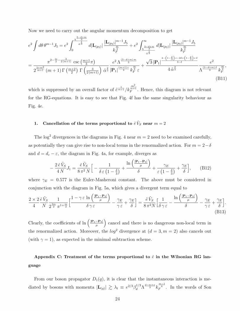
1. Cancellation of the terms proportional to e VS near m = 2

The log2 divergences in the diagrams in Fig. 4 near m = 2 need to be examined carefully,

as potentially they can give rise to non-local terms in the renormalized action. For m = 2−δand d = dc − ε, the diagram in Fig. 4a, for example, diverges as

− 2 e VS4N

J1 =e VS

8 π2N

[− 1

δ ε(1− δ

3

) +ln(|P1−P3|

µ

)δ

+γE

ε(1− δ

3

) +γEδ

], (B12)

where γE = 0.577 is the Euler-Masheroni constant. The above must be considered in

conjunction with the diagram in Fig. 5a, which gives a divergent term equal to

2× 2

4

e VSN

1

23m2 π1+m

2

[1− γ ε ln(|P1−P3|

µ

)δ γ ε

− γEγ ε

+γEδ

]=

e VS8π2N

[ 1

δ γ ε−

ln(|P1−P3|

µ

)δ

− γEγ ε

+γEδ

].

(B13)

Clearly, the coefficients of ln(|P1−P3|

µ

)cancel and there is no dangerous non-local term in

the renormalized action. Moreover, the log2 divergence at (d = 3,m = 2) also cancels out

(with γ = 1), as expected in the minimal subtraction scheme.

Appendix C: Treatment of the terms proportional to e in the Wilsonian RG lan-

guage

From our boson propagator D1(q), it is clear that the instantaneous interaction is me-

diated by bosons with momenta |L(q)| & λt ≡ e2/3β1/3d Λ

d−m+x3 k

m−16

F . In the words of Son

24

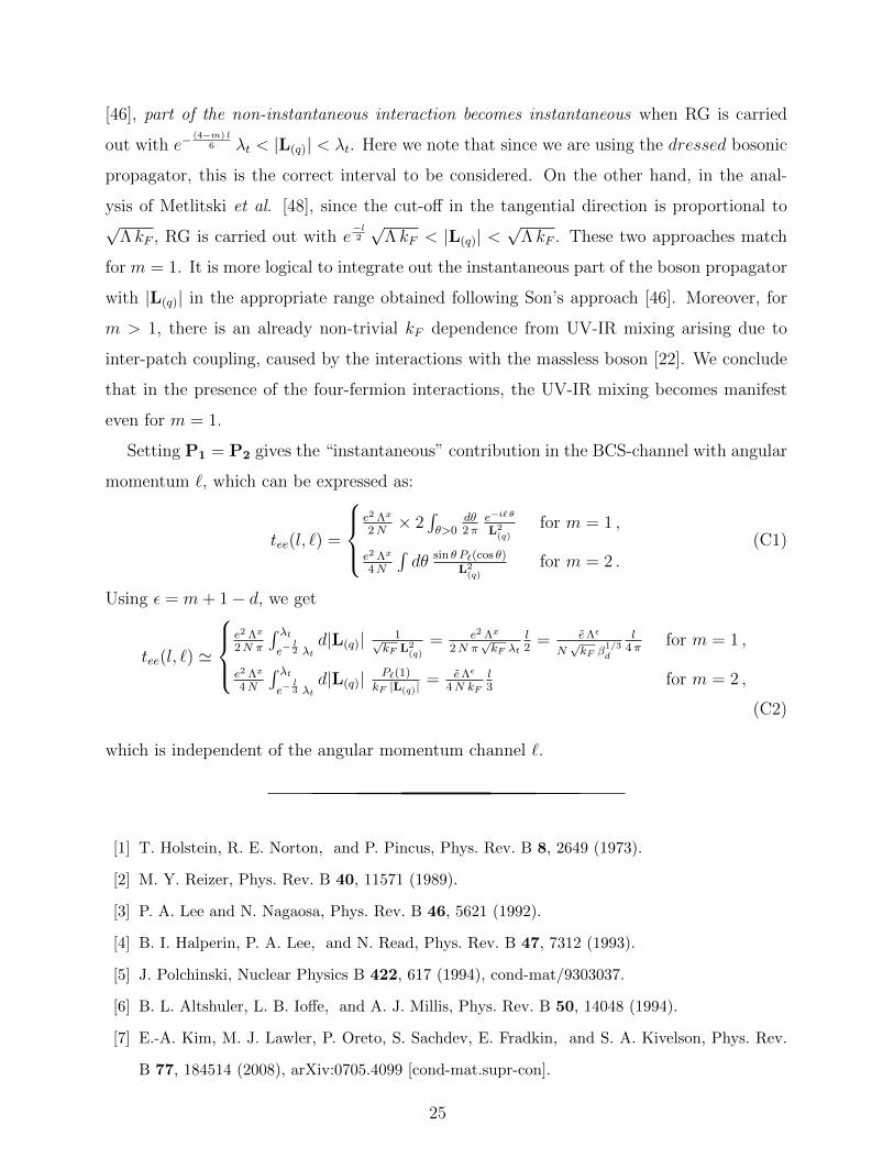
[46], part of the non-instantaneous interaction becomes instantaneous when RG is carried

out with e−(4−m) l

6 λt < |L(q)| < λt. Here we note that since we are using the dressed bosonic

propagator, this is the correct interval to be considered. On the other hand, in the anal-

ysis of Metlitski et al. [48], since the cut-off in the tangential direction is proportional to√

Λ kF , RG is carried out with e−l2

√Λ kF < |L(q)| <

√Λ kF . These two approaches match

for m = 1. It is more logical to integrate out the instantaneous part of the boson propagator

with |L(q)| in the appropriate range obtained following Son’s approach [46]. Moreover, for

m > 1, there is an already non-trivial kF dependence from UV-IR mixing arising due to

inter-patch coupling, caused by the interactions with the massless boson [22]. We conclude

that in the presence of the four-fermion interactions, the UV-IR mixing becomes manifest

even for m = 1.

Setting P1 = P2 gives the “instantaneous” contribution in the BCS-channel with angular

momentum `, which can be expressed as:

tee(l, `) =

e2 Λx

2N× 2

∫θ>0

dθ2π

e−i` θ

L2(q)

for m = 1 ,

e2 Λx

4N

∫dθ sin θ P`(cos θ)

L2(q)

for m = 2 .(C1)

Using ε = m+ 1− d, we get

tee(l, `) '

e2 Λx

2N π

∫ λte−

l2 λt

d|L(q)| 1√kF L2

(q)

= e2 Λx

2N π√kF λt

l2

= eΛε

N√kF β

1/3d

l4π

for m = 1 ,

e2 Λx

4N

∫ λte−

l3 λt

d|L(q)| P`(1)kF |L(q)|

= eΛε

4N kF

l3

for m = 2 ,

(C2)

which is independent of the angular momentum channel `.

[1] T. Holstein, R. E. Norton, and P. Pincus, Phys. Rev. B 8, 2649 (1973).

[2] M. Y. Reizer, Phys. Rev. B 40, 11571 (1989).

[3] P. A. Lee and N. Nagaosa, Phys. Rev. B 46, 5621 (1992).

[4] B. I. Halperin, P. A. Lee, and N. Read, Phys. Rev. B 47, 7312 (1993).

[5] J. Polchinski, Nuclear Physics B 422, 617 (1994), cond-mat/9303037.

[6] B. L. Altshuler, L. B. Ioffe, and A. J. Millis, Phys. Rev. B 50, 14048 (1994).

[7] E.-A. Kim, M. J. Lawler, P. Oreto, S. Sachdev, E. Fradkin, and S. A. Kivelson, Phys. Rev.

B 77, 184514 (2008), arXiv:0705.4099 [cond-mat.supr-con].

25

[8] C. Nayak and F. Wilczek, Nuclear Physics B 430, 534 (1994), cond-mat/9408016.

[9] M. J. Lawler, D. G. Barci, V. Fernandez, E. Fradkin, and L. Oxman, Phys. Rev. B 73, 085101

(2006), cond-mat/0508747.

[10] M. J. Lawler and E. Fradkin, Phys. Rev. B 75, 033304 (2007), cond-mat/0605203.

[11] S.-S. Lee, Phys. Rev. B 80, 165102 (2009).

[12] M. A. Metlitski and S. Sachdev, Phys. Rev. B 82, 075127 (2010).

[13] M. A. Metlitski and S. Sachdev, Phys. Rev. B 82, 075128 (2010).

[14] A. Abanov and A. Chubukov, Physical Review Letters 93, 255702 (2004).

[15] A. Abanov and A. V. Chubukov, Physical Review Letters 84, 5608 (2000), cond-mat/0002122.

[16] A. Abanov, A. V. Chubukov, and J. Schmalian, Advances in Physics 52, 119 (2003).

[17] D. F. Mross, J. McGreevy, H. Liu, and T. Senthil, Phys. Rev. B 82, 045121 (2010).

[18] H.-C. Jiang, M. S. Block, R. V. Mishmash, J. R. Garrison, D. N. Sheng, O. I. Motrunich, and

M. P. A. Fisher, Nature (London) 493, 39 (2013), arXiv:1207.6608 [cond-mat.str-el].

[19] S. Sur and S.-S. Lee, Phys. Rev. B 90, 045121 (2014).

[20] D. Dalidovich and S.-S. Lee, Phys. Rev. B 88, 245106 (2013).

[21] S. Sur and S.-S. Lee, Phys. Rev. B 91, 125136 (2015).

[22] I. Mandal and S.-S. Lee, Phys. Rev. B 92, 035141 (2015).

[23] I. Mandal, ArXiv e-prints (2016), arXiv:1608.06642 [cond-mat.str-el].

[24] A. Eberlein, I. Mandal, and S. Sachdev, Phys. Rev. B 94, 045133 (2016).

[25] V. Oganesyan, S. A. Kivelson, and E. Fradkin, Phys. Rev. B 64, 195109 (2001).

[26] W. Metzner, D. Rohe, and S. Andergassen, Phys. Rev. Lett. 91, 066402 (2003).

[27] L. Dell’Anna and W. Metzner, Phys. Rev. B 73, 045127 (2006).

[28] L. Dell’Anna and W. Metzner, Phys. Rev. Lett. 98, 136402 (2007).

[29] H.-Y. Kee, E. H. Kim, and C.-H. Chung, Phys. Rev. B 68, 245109 (2003).

[30] J. Rech, C. Pepin, and A. V. Chubukov, Phys. Rev. B 74, 195126 (2006).

[31] P. Wolfle and A. Rosch, Journal of Low Temperature Physics 147, 165 (2007), cond-

mat/0609343.

[32] D. L. Maslov and A. V. Chubukov, Phys. Rev. B 81, 045110 (2010).

[33] J. Quintanilla and A. J. Schofield, Phys. Rev. B 74, 115126 (2006), cond-mat/0601103.

[34] H. Yamase and H. Kohno, Journal of the Physical Society of Japan 69, 2151 (2000).

[35] H. Yamase, V. Oganesyan, and W. Metzner, Phys. Rev. B 72, 035114 (2005).

26

[36] C. J. Halboth and W. Metzner, Phys. Rev. Lett. 85, 5162 (2000).

[37] P. Jakubczyk, P. Strack, A. A. Katanin, and W. Metzner, Phys. Rev. B 77, 195120 (2008).

[38] M. Zacharias, P. Wolfle, and M. Garst, Phys. Rev. B 80, 165116 (2009).

[39] Y. Huh and S. Sachdev, Phys. Rev. B 78, 064512 (2008), arXiv:0806.0002 [cond-mat.str-el].

[40] O. I. Motrunich, Phys. Rev. B 72, 045105 (2005), cond-mat/0412556.

[41] S.-S. Lee and P. A. Lee, Phys. Rev. Lett. 95, 036403 (2005).

[42] P. A. Lee, N. Nagaosa, and X.-G. Wen, Reviews of Modern Physics 78, 17 (2006).

[43] O. I. Motrunich and M. P. A. Fisher, Phys. Rev. B 75, 235116 (2007).

[44] L. Yin and S. Chakravarty, International Journal of Modern Physics B 10, 805 (1996), cond-

mat/9511085.

[45] T. Senthil, Phys. Rev. B 78, 035103 (2008).

[46] D. T. Son, Phys. Rev. D 59, 094019 (1999).

[47] S. B. Chung, I. Mandal, S. Raghu, and S. Chakravarty, Phys. Rev. B 88, 045127 (2013).

[48] M. A. Metlitski, D. F. Mross, S. Sachdev, and T. Senthil, Phys. Rev. B 91, 115111 (2015).

[49] Z. Wang, I. Mandal, S. B. Chung, and S. Chakravarty, Annals of Physics 351, 727 (2014).

[50] S. Raghu, G. Torroba, and H. Wang, Phys. Rev. B 92, 205104 (2015).

[51] S. Chakravarty, R. E. Norton, and O. F. Syljuasen, Physical Review Letters 74, 1423 (1995).

[52] A. L. Fitzpatrick, S. Kachru, J. Kaplan, and S. Raghu, Phys. Rev. B 88, 125116 (2013).

[53] A. L. Fitzpatrick, S. Kachru, J. Kaplan, and S. Raghu, Phys. Rev. B 89, 165114 (2014).

[54] R. Mahajan, D. M. Ramirez, S. Kachru, and S. Raghu, Phys. Rev. B 88, 115116 (2013).

[55] G. Torroba and H. Wang, Phys. Rev. B 90, 165144 (2014).

[56] T. Senthil and R. Shankar, Phys. Rev. Lett. 102, 046406 (2009).

[57] We would like to emphasize that (d = 3,m = 2) Fermi liquids are also unstable to Cooper

pairing for an infinitesimally weak interaction regardless of its sign, but in some higher angular

momentum channel (` > 0) [58]. For the Ising-nematic case under study, such an instability

occurs for all angular momentum channels.

[58] W. Kohn and J. M. Luttinger, Phys. Rev. Lett. 15, 524 (1965).

27