6

Time-Dependent Greenhouse-Gas-Induced Climate Change

F.P. BRETHERTON, K. BRYAN, J.D. WOODS

Contributors: /. Hansen; M. Hoffert; X. Jiang; S. Manabe; G. Meehl; S.C.B. Raper; D. Rind; M. Schlesinger; R. Stouffer; T. Volk; T.M.L. Wigley.

CONTENTS

Executive Summary 177

6.1 Introduction 179 6.1.1 Why Coupled Ocean-Atmosphere Models ? 179 6.1.2 Types of Ocean Models 179 6.1.3 Major Sources of Uncertainty 180

6.2 Expectations Based on Equilibrium Simulations 180

6.3 Expectations Based on Transient Simulations 181

6.4 Expectations Based on Time-Dependent Simulations 181

6.4.1 Changes in Surface Air Temperature 181 6.4.2 Changes in Soil Moisture 183

6.5 An Illustrative Example 183 6.5.1 The Experiment 183 6.5.2 Results 184 6.5.3 Discussion 185 6.5.4 Changes in Ocean Circulation 187

6.6 Projections of Future Global Climate Change 187 6.6.1 An Upwelling Diffusion Model 187 6.6.2 Model Results 188

6.6.3 Discussion 190

6.7 Conclusions 191

References 192

EXECUTIVE SUMMARY

The slowly changing response of climate to a gradual increase in

greenhouse gas concentrations can only be modelled ngourously

using a coupled ocean-atmosphere general circulation model with

full ocean dynamics This has now been done by a small number

of researchers using coarse resolution models out to 100 years

Their results show that

a) For a steadily increasing forcing, the global rise in

temperature is an approximately constant fraction of the

equilibrium rise corresponding to the instantaneous forcing

for a time that is earlier by a fixed offset For an

atmospheric model with temperature sensitivity 4°C for a

doubling of CO2, this fraction is approximately 66% with

an offset of 11 years In rough terms, the response is about

60% of the current equilibrium value Extrapolation using

robust scaling principles indicates that for a sensitivity of

1 5°C the corresponding values are 85% 6 years and 80%

respectively

b) The regional patterns of temperature and precipitation

change generally resemble those of an equilibrium

simulation for an atmospheric model, though uniformly

reduced in magnitude Exceptional regions are around

Antarctica and in the northern North Atlantic, where the

warming is much less

c) These results are generally consistent with our

understanding of the present circulation in the ocean, as

evidenced by geochemical and other tracers However,

available computer power is still a serious limitation on

model capability, and existing observational data are

inadequate to resolve basic issues about the relative roles of

various mixing processes, thus affecting the confidence

level that can be applied to these simulations

d) The conclusions about the global mean can be extended

though with some loss of rigour, by using a simple energy

balance climate model with an upwelling diffusion model

of the ocean, similar to that used to simulate CO2 uptake

It is inferred that, if a steadily increasing greenhouse

forcing were abruptly stabilized to a constant value

thereafter, the global temperature would continue to rise at

about the same rate for some 10-20 years, following which

it would increase much more slowly approaching the

equilibrium value only over many centuries

e) Based on the IPCC Business as Usual scenarios, the

energy-balance upwelling diffusion model with best

judgement parameters yields estimates of global warming

from pre-industrial times (taken to be 1765) to the year

2030 between 1 3°C and 2 8"C, with a best estimate of

2 0°C This corresponds to a predicted rise trom 1990 of

0 7-1 5°C with a best estimate of 1 1"C

Temperature rise from pre-industrial times to the year 2070 is

estimated to be between 2 2°C and 4 8°C with a best estimate of

3 3°C This corresponds to a predicted rise from 1990 of 1 6°C to

3 5°C, with a best estimate of 2 4°C

6 Time-Dependent Gi eenhoute-Gas Induced Climate Change 179

6.1 Introduction

6.7.7 Why Coupled Ocean-Atmosphere Models ? The responses discussed in Section 5 are for a radiative forcing that is constant for the few years required for the atmosphere and the surface of the ocean to achieve a new equilibrium following an abrupt change Though the atmospheric models are detailed and highly developed, the treatment of the ocean is quite primitive However, when greenhouse gas concentrations are changing continuously, the thermal capacity of the oceans will delay and effectively reduce the observed climatic response At a given time, the realized global average temperature will reflect only part of the equilibrium change for the corresponding instantaneous value of the forcing Of the remainder, part is delayed by storage in the stably stratified layers of the upper ocean and is realized within a few decades or perhaps a century, but another part is effectively invisible for many centuries or longer, until the heating of the deep ocean begins to influence surface temperature In addition, the ocean currents can redistribute the greenhouse warming spatially, leading to regional modifications of the equilibrium computations Furthermore, even without changes in the radiative forcing, interactions between the ocean and atmosphere can cause mterannual and mter-decadal fluctuations that can mask longer term climate change for a while

To estimate these effects, and to make reliable predictions of climate change under realistic scenarios of increasing forcing, coupled atmosphere-ocean general circulation models (GCMs) are essential Such models should be designed to simulate the time and space dependence of the basic atmospheric and oceanic variables, and the physical processes that control them, with enough fidelity and resolution to define regional changes over many decades in the context of year to year variability In addition, the reasons for differences between the results of different models should be understood

6.1.2 Types of Ocean Models The ocean circulation is much less well observed than the atmosphere, and there is less confidence in the capability of models to simulate the controlling processes As a result, there are several conceptually different types of ocean model in use for studies of greenhouse warming

The simplest representation considered here regards the ocean as a body with heat capacity modulated by down­ward diffusion below an upper mixed layer and a horizontal heat flux divergence within the mixed layer These vary with position, but are prescribed with values that result, in association with a particular atmosphcnc model running under present climatic conditions in simulations which fit observations loi the annual mean surface temperature, and the annual cycle about that mean

In such a no surprises ocean (Hansen et al , 1988) the horizontal currents do not contribute to modifications of climate change

A more faithful representation is to treat the additional heat associated with forcing by changing greenhouse gases as a passive tracer which is advected by three-dimensional currents and mixed by specified diffusion coefficients intended to represent the sub-grid scale processes These currents and mixing coefficients may be obtained from a GCM simulating the present climate and ocean circulation, including the buoyancy field, in a dynamically consistent manner Using appropriate sources, the distributions ol transient and other tracers such as temperature-salinity relationships, 14C, tritium and CFCs are then inferred as a separate, computationally relatively inexpensive, step and compared with observations Poorly known parameters such as the horizontal and vertical diffusion coefficients are typically adjusted to improve the fit In box-diffusion models, which generally have a much coarser resolution, the currents and mixing are inferred directly from tracer distributions or are chosen to represent the aggregated effect of transports within a more detailed GCM Though potential temperature (used to measure the heat content per unit volume) affects the buoyancy of sea-water and hence is a dynamically active variable, a number of studies (e g , Bryan et al , 1984) have demonstrated that small, thermally driven, perturbations in a GCM do in fact behave in the aggregate very much as a passive tracer This approach is useful for predicting small changes in climate from the present, in which the ocean currents and mixing co­efficients themselves are assumed not to vary in a significant manner There are at present no clear guidelines as to to what is significant for this purpose

A complete representation requires the full power of a high resolution ocean GCM, with appropriate boundary conditions at the ocean surface involving the wind stress, net heat flux and net freshwater flux obtained from an atmospheric model as a function oi time in exchange for a simulation of the ocean surface temperature The explicit simulation of mixing by mesoscale eddies is feasible and highly desirable (Semtner and Chervin 1988), but it requires high spatial resolution, and so far the computer capacity required for 100 year simulations on a coupled global eddy resolving ocean-atmosphere GCM has not been available Sea-ice dynamics are needed as well as thermodynamics, which is highly parameterized in existing models For a fully credible climate prediction what is required is such a complete, dynamically consistent representation, thoroughly tested against observations

General circulation models ol the coupled ocean atmosphere system have been under development for many years but they have been restricted to coarse resolution models in which the mixing coefficients in the ocean must

1X0 Time-Dependent Gi eenhouse-Gai-Induced Climate Change 6

be prescribed ad hoc, and other unphysical devices are needed to match the ocean and atmospheric components Despite these limitations, such models are giving results that seem consistent with our present understanding of the broad features of the ocean circulation, and provide an important tool for extending the conclusions of the equilibrium atmospheric climate models to time dependent situations, at least while the ocean circulation does not vary greatly from the present

Because running coupled ocean-atmosphere GCMs is expensive and time consuming many of our conclusions about global trends in future climates are based upon simplified models, in which parts of the system are replaced by highly aggregated constructs in which key formulae are inferred from observations or from other, non-mtcractive, models An energv, -balance atmospheric model coupled to a one dimensional upwelhng-ditfusion model of the ocean provides a useful conceptual framework, using a tracer representation to aid the interpretation of the results of the GCMs, as well as a powerful tool for quickly exploring future scenarios of climate change

6.1.3 Major Sources of Uncertainty An unresolved question related to the coarse resolution of general circulation models i the extent to which the details of the mixing processes and ocean currents may affect the storage of heat on different time scales and hence the traction of the equilibrium global temperature rise that is realized only after several decades as opposed to more quickly or much more slowlv Indeed this issue rests in turn on questions whether the principal control mechanisms governing the sub-grid scale mixing are correctly incorporated For a more detailed discussion see Section 48

Paralleling these uncertainties are serious limitations on the observational data base to which all these models are compared, and from which the present rates of circulation are inferred These give rise to conceptual differences of opinion among oceanographers about how the circulation actually functions

Existing observations of the large scale distribution of temperature, salinity and other geochemical tracers such as tritium and 14C do indicate that near surface water sinks deep into the water column to below the main thermochne, primarily in restricted regions in high latitudes in the North Atlantic and around the Antarctic continent Associated with these downwelling regions, but not not necessarily co-located, are highly localized patches of intermittent deep convection, or turbulent overturning of a water column that is gravitationally unstable Though controlled to a sig­nificant extent by salinity variations rather than by temperature, this deep convection can transfer heat vertically very rapidly

However, much less clear is the return path of deep water to the ocean surface through the gravitationally stable thermochne which covers most of the ocean It is disputed whether the most important process is nearly horizontal motion bulk motion in sloping isopycnal surfaces of constant potential density, ventilating the thermochne laterally In this view, significant mixing across isopyncal surfaces occurs only where the latter intersect with the well mixed layer just below the ocean-atmosphere interface, which is stirred from above by the wind and by surface heat and water fluxes (Woods, 1984) Another view, still held by some oceanogiaphers, is that the dominant mechanism is externally driven in situ mixing in a gravitationally stable environment and can be described by a local bulk diffusivity To obtain the observations necessary to describe more accurately the real ocean circulation, and to improve our ability to model it for climate purposes, the World Ocean Circulation Experiment is currently underway (see Section 11)

6.2 Expectations Based on Equilibrium Simulations

Besides the different types of model, it is important also to distinguish the different experiments that have been done with them

With the exception of the few time-dependent simulations described in Sections 6 3 - 6 6 , perceptions of the geographical patterns of CC>2-induced climate change have been shaped mainly by a generation of atmospheric GCMs coupled to simple mixed layer or slab ocean models (see review by Schlesinger and Mitchell, 1987) With these specified-depth mixed-layer models having no computed ocean heat transport, CO2 was instantaneously doubled and the models run to equilibrium Averages taken at the end of the simulations were used to infer the geographical patterns of CO? induced climate change (Section 5)

Generally, the models agreed among themselves in a qualitative sense Surface air temperature increase was greatest in late autumn at high latitudes in both hemispheres, particularly over regions covered by sea-ice This was associated with a combination of snow/sea-ice albedo feedback and reduced sea-ice thermal inertia Soil moisture changes showed a tendency for drying of mid-continental regions in summer, but the magnitude and even the sign of the change was not uniform among the models (see also Section 5 2 2 3) This inconsistency is caused by a number of factors Some had to do with how soil moisture amounts were computed in the control sim­ulations (Meehl and Washington, 1988), and some had to do with the method of simulating the land surface (Rind et al , 1989) Also, all models showed a strong cooling in the lower stratosphere due to the radiative effects of the increased carbon dioxide

6 Time Dependent Gi eenhouse Gas-Indue ed Climate Change 1H1

Recently, a new generation of coupled models has been run with atmospheric GCMs coupled to coarse-grid, dynamical ocean GCMs These models include realistic geography, but the coarse grid of the ocean part (about 500 km by 500 km) necessitates the parameterization of mesoscale ocean eddies through the use of horizontal heat diffusion This and other limitations involved with such an ocean model are associated with a number of systematic errors in the simulation (e g , Meehl, 1989) However, the ability to include an explicitly computed ocean heat transport provides an opportunity to study, for the first time, the ocean's dynamical effects on the geographical patterns of CC>2-induced climate change

6.3 Expectations Based on Transient Simulations

The first simulations with these global, coupled GCMs applied to the CO~2 problem used the same methodology as that employed in the earlier simple mixed-layer models That is, CO"2 was doubled instantaneously and the model run for some time-period to document the climate changes It has been suggested, however, that because of the long thermal response time ot the full ocean, and the fact that the warming penetrates downward from the ocean surface into its interior, the traditional concept of a sensitivity experiment to determine a new equilibrium may be less useful with such a coupled system (Schlesinger and Jiang, 1988)

Schlesinger et al (1985) ran a two-level atmospheric model coupled to a 6-layer ocean GCM for 20 years after instantaneously doubling CCb They noted that the model could not have attained an equilibrium in that period, and went on to document changes in climate at the end of the experiment Washington and Meehl (1989) performed a similar experiment over a 30 year period with inst­antaneously doubled CO~2 in their global spectral atmospheric GCM coupled to a coarse-grid ocean GCM Manabe et al (1990) also used a global spectral atm­ospheric GCM coupled to a coarse-grid ocean model in an instantaneous CO2 doubling experiment for a 60-year period

These model simulations have been referred to as transient experiments in the sense that the time evolution of the whole climate system for a prescribed 'switch-on' instantaneous CO2 doubling could be examined in a meaningful way

In some respects, all the switch-on coupled GCM experiments agree with the earlier mixed-layei iesults In the Northern Hemisphere, warming is larger at higher latitudes, and there is some evidence, though again mixed of drying in the mid-continental regions in summer Manabe et al (1990) also obtained a wetter soil in middle latitudes in winter In the summer however, Manabe et al (1990) found large areas in the middle latitudes where the

soil was drier However, sector-configuration simulations (Bryan et al , 1988) with a coupled GCM hrst suggested a major difference in the patterns of climate change compared with the earlier mixed-layer model experiments Around Antarctica, a relative warming minimum, at times even a slight cooling, was evident in these simulations

6.4 Expectations Based on Time-Dependent Simulations

The term time-dependent in the present context is taken to mean a model simulation with gradually increasing amounts of greenhouse gases This is what is happening in the real climate system, and such simulations provide us with the first indication of the climate-change signals we may expect in the near future

To date, three such simulations have been published One has been performed with an atmospheric model coupled to a simple ocean with fixed horizontal heat transport (Hansen et al , 1988), and the other two have used atmospheric models coupled to coarse-grid dynamical ocean models, that is, atmosphere-ocean GCMs (Washington and Meehl, 1989, Stouffer et al , 1989) Other studies using coupled ocean-atmosphere GCMs are in progress at the UK Meteorological Of lice (Hadley Centre) and the Max Plank Institute fur Meteorologie, Hamburg

6.4.1 Changes In Surface Air Temperature Hansen et al (1988) performed several simulations with CO2 and other greenhouse gases increasing at various rates, aimed at assessing the detectability ol a wanning trend above the inherent variability of a coupled ocean-atmosphere system The ocean model was a no surprises ocean as described in Section 6 1 2, which simulates the spatially varying heat capacity typical of present climate but precludes leedback to climate change lrom the ocean currents At any given time the simulated wanning was largest in the continental interior of Asia and at the high latitudes of both hemispheres, though it was first unambiguous in the tropics where the interannual variability is least Contrasting with some othci sim­ulations, regional patterns of climate anomalies also had a tendency to show greater warming in the central and southeast U S , and less warming in the western U S The Antarctic also warmed about as much as conespondmg northern high latitudes, a result that may be sensitive to the assumptions about ocean heat transport in this model

Washington and Meehl (1989) specified a V/< per year Iincui increase of CO2 in then coupled atmosphere-ocean GCM over a 30-year period and documented changes in the ocean-atmosphere system For this period there was a tendency for the land areas to warm faster than the oceans and foi the warming to be larger in the surface layci of the

182 Time-Dependent Gieenhouse-Gas-Induced Climate Change 6

ocean than below Significant areas of ocean surface temperature increase tended to occur between 50°S and 30°N (Figure 6.1). Warming was smaller and less significant around Antarctica. In the high latitudes of the Northern Hemisphere there was no zonally consistent warming pattern, in contrast to the earlier mixed-layer experiments. In fact, there was a cooling in the North Atlantic and Northwest Pacific for the particular five-year period shown in Figure 6.1. Washington and Meehl (1989) show that this cooling was a consequence of alterations in atmospheric and ocean circulation involving changes in precipitation and a weakening of the oceanic thermohahne circulation However, there was a large inter-annual variability at high latitudes in the model, as occurs in nature, and Washington and Meehl pointed out that the pattern for this five-year period was indicative only of coupled anomalies that can occur in the system. Nevertheless, similar patterns of observed climate anomalies have been documented for temperature trends over the past 20-year period in the Northern Hemisphere (Karoly, 1989; Jones et al., 1988).

Stouffer et al. (1989) performed a time-dependent experiment with CO2 increasing 1% per year (compounded), and documented geographical patterns of temperature differences for years 61-70. Stouffer et al (1989) show the continents warming faster than the oceans, and a significant warming minimum near 60°S around Antarctica, as was seen in earlier sector experiments (Bryan et al., 1988). As was also seen in the Washington and Meehl results, there was not a uniform pattern of warming at all longitudes at high latitudes in the Northern Hemisphere A minimum of warming occurred in the northwestern North Atlantic in association with deep overturning of the ocean. Though the greatest warming occurred at high latitudes of the Northern Hemisphere, the greater variability there resulted in the warming being unambiguously apparent first in the subtropical ocean regions.

The main similarities in the geographical patterns of C02-induced temperature change among these three time-dependent experiments are:

AT991 DJF, transient minus control, (yr 26—30)

AT991 JJA transient minus control (yr 26—30)

Figure 6.1: Geographical distributions ot the surface temperatuie difference, transient minus control, of years 26-30 for (a) DJF and (b) JJA (°C. lowest model layer) Differences significant at Wr level are hatched Adapted from Washington and Meehl (1989)

6 Time Dependent Gi eenhouse Gas Induced Climate Change 183

1) the warming at any given time is less than the corresponding equilibrium value for that inst­antaneous forcing,

2) the areas of warming are generally greater at high latitudes in the Northern Hemisphere than at low latitudes, but are not zonally uniform in the earlier stages of the time-dependent experiments, and

3) because of natural variability, statistically significant warming is most evident over the subtropical oceans

The differences between the time-dependent experiment using specified ocean heat transports (Hansen et al , 1988) and the two time dependent experiments with dynamical ocean models (Washington and Meehl, 1989, Stouffer et al, 1989) are

1) a warming minimum (or slight cooling) around Antarctica in the models with a dynamical ocean precludes the establishment of the large, positive ice-albedo feedback that contributes to extensive southern high-latitude warming in the mixed-layer models, and

2) a warming minimum in the northern North Atlantic

These local minima appear to be due to exchange of the surface and deep layers of the ocean associated with upwelhng as well as downwelling, or with convective overturning The downwelling ot surface water in the North Atlantic appears to be susceptible to changes of atmospheric circulation and precipitation and the attendant weakening of the oceanic thermohahne circulation

6.4.2 Changes In Soil Moisture As indicated in Section 4 5, large-scale precipitation patterns are very sensitive to patterns of sea-surface temperature anomalies Rind et al (1989) link the occ­urrence of droughts with the climate changes in the time-dependent simulations of Hansen et al (1988), and predict increased droughts by the 1990s Washington and Meehl (1989) found in their time-dependent experiment that the soil in mid-latitude continents was wetter in winter and had small changes of both signs in summer These time dependent results are consistent with the results from their respective equilibrium climate change simulations (Section 5) A full analysis of the experiment described in Stouffer et al (1989) is not yet available, but preliminary ind­ications (Manabe, 1990) are that they are similarly consistent, though there may be some small changes in global scale patterns

6.5 An Illustrative Example

In this section, we illustrate the promise and limitations of interactive ocean-atmosphere models with more details of one of the integrations described in Section 6 4 drawing on

Stouffer et al (1989) and additional material supplied by Manabe (1990)

6.5.1 The Experiment Three 100-year simulations are compared with different radiative forcing, each starting from the same, balanced initial state The concentration of atmospheric carbon dioxide is kept constant in a control run In two complementary perturbation runs the concentration ol atmospheric carbon dioxide is increased or decreased by 1% a year (compounded) implying a doubling or halving after 70 years This Iate of increase roughly corresponds in terms of CO? equivalent units to the present rate ol increase of forcing by all the greenhouse gases Since greenhouse warming is proportional to the logarithm ol carbon dioxide concentration (see Section 2, Table 2 2 4 1) an exponential increase gives a linear increase in radiative forcing

To reach the initial balanced state the atmosphenc model is lorced to a steady state with the annual mean and seasonal variation of sea surface temperature given by climatological data Using the seasonally varying winds fiom the atmospheric model the ocean is then foiccd to a balanced state with the sea surface temperature and sea surface salinity specified from climatological data For models perfectly representing the present climate and assuming the climatological data are accurate the fluxes of heat and moisture should agree exactly In practice the models are less than perfect and the heat and moisture flux fields at the ocean surface have a substantial mismatch

To compensate for this mismatch when the two models are coupled an ad hot (lux adjustment is added to the atmosphenc heat and moisture fluxes This flux ad] ustment which is a fixed function of position and season is precisely the concction icquired so that as long as the radiative forcing of the atmosphenc model icmains the same the coupled model will iemain balanced and fluctuate around a mean state that includes the obseived sea surface temperature and sea surlace salinity When the radiative balance ot the atmospheric model is peiturbed the coupled model is free to seek a new equilibrium because the ad hot flux adjustments remain as specified and provide no constraint to damp out depaituies fiom the present climate

The flux adjustments in this treatment are nonphysical and disconcertingly large (Manabe 1990) but are simply a symptom of the inadequacies in the separate models and ol a mismatch between them Unfoitunately existing mea surements of ocean surface fluxes are quite inadequate to determine the precise causes This device or its equivalent (eg Sausen et al 1988) is the price that must be paid lor a controlled simulation ol perturbations from a realistic present day, ocean atmosphere climate Though varying through the annual cycle the pattern of adjustment is the

184 Time Dependent Gi eenhouse Gas-Indiued Climate Change 6

mean surface air temperature within the control run itself (Figure 6 2) These imply a standard deviation in decadal averages of about ±0 08°C, which, though an accurate representation of the model climatology, appears to be somewhat less than what has been observed during the past 100 years (see Section 8) The regional manifestation shown in Figure 6 3 illustrates the uncertainty that is inherent in estimates of time dependent regional climate change ovei 20 year periods

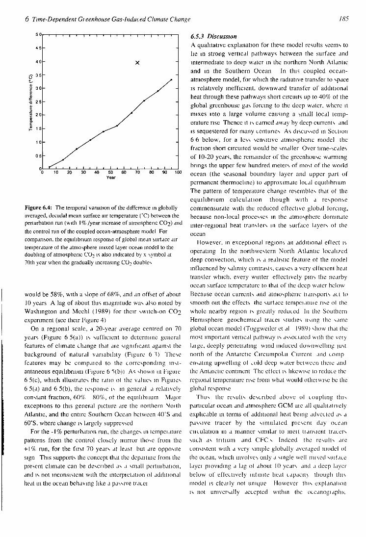
Figure 6 4 shows the difference in 10-year, global average surface air temperature, between the +1% pert­urbation run and the long term average of the control run, increasing approximately linearly as a function of time After 70 years, the instantaneous temperature is only 58% of the equilibrium value (4°C, see Wetherald and Manabe, 1988) appropriate to the radiative forcing at that time This result compares reasonably well with the estimate of 55% obtained by running the box diffusion model ol Section 6 6 with similar scenario of radiative forcing and a climate sensitivity of 4°C for a doubling of CO2 (see Figure 6 7 later) However a result ol both simulations is that the response to a linear increase in forcing with time is also, after a brief initial phase very close to linear in time The time dependent response is thus at all times proportional to the instantaneous forcing, but at a reduced magnitude compared to the equilibrium Close examination of Figures 6 4 and 6 7 show that a straight line fit to the response intersects the time axis at ten years Since lag in the response increases with time it is not a useful parameter to describe results As an alternative, the response is described in terms of a fraction of the equilibrium forcing which corresponds to a time with fixed offset to ten years earlier Thus in the case of Figure 6 4, the fractional response

STANDARD DEVIATION OF 20 YEAR MEAN CONTROL RUN TEMPERATURE

Figure 6.3: The geographic distribution ol the standard deviation ol 20 year mean surface air temperatures in the control run From Manabe (1990) personal communication

§ +0 2

40 60 Years

Figure 6.2: The temporal variation ot the deviation of global mean surface air temperature (°C) of the coupled ocean atmosphere model from its long term average From Manabe (1990), personal communication

same in all three simulations Its direct effects thus disappear when differences are considered, and the con­clusions from such experiments should be reasonable provided the differences remain small However, when the simulated ocean circulation or atmospheric state differs greatly from that presently observed, indirect effects are likely to be substantial and too much credence should not be attached to the results There are currently no quantitative criteria for what differences should be regarded as small for this purpose

6.5.2 Results Before examining the changes due to greenhouse forcing, it is instructive to note the random fluctuations in global

6 Time-Dependent Gi eenhouse Gas-Induced Climate Change 185

Figure 6.4: The temporal variation of the difference in globally averaged, decadal mean surface air temperature (°C) between the perturbation run (with 1 % /year increase of atmospheric CO2) and the control run of the coupled ocean-atmosphere model For comparison, the equilibrium response of global mean surface air temperature ot the atmosphere mixed layer ocean model to the doubling of atmospheric CO2 is also indicated by x symbol al 70th year when the gradually increasing CO? doubles

would be 58%, with a slope of 68%, and an offset of about 10 years A lag of about this magnitude was also noted by Washington and Meehl (1989) for their switch-on CO2 experiment (see their Figure 4)

On a regional scale, a 20-year average centred on 70 years (Figure 6 5(a)) is sufficient to determine general features of climate change that aie significant against the background of natural variability (Figure 6 T) These features may be compaied to the corresponding inst­antaneous equilibrium (Figure 6 5(b)) As shown in Figuie 6 5(c), which illustrates the ratio ol the values in Figuies 6 5(a) and 6 5(b), the lesponse is in general a relatively constant fraction, 60% 80%, ot the equilibnum Major exceptions to this general picture are the northern Noith Atlantic, and the entire Southern Ocean between 40°S and 60°S, where change is largely suppressed

For the - 1 % perturbation run, the changes in tempciature patterns from the control closely mirror those from the + 1% run, for the first 70 years at least but are opposite sign This supports the concept that the depaituie from the present climate can be described as a small pertuibation, and is not inconsistent with the interpietation of additional heat in the ocean behaving like a passive tracei

6.5.3 Discussion A qualitative explanation for these model results seems to lie in strong vertical pathways between the surface and intermediate to deep water in the northern North Atlantic and in the Southern Ocean In this coupled ocean-atmosphere model, for which the radiative transfer to space is relatively inefficient, downward transfer of additional heat through these pathways short circuits up to 40% of the global greenhouse gas forcing to the deep water, where it mixes into a large volume causing a small local temp­erature rise Thence it is carried away by deep currents and is sequestered for many centuries As discussed in Section 6 6 below, for a less sensitive atmospheric model the fraction short circuited would be smaller Over time-scales of 10-20 years, the remainder of the greenhouse warming brings the upper few hundred meters of most of the world ocean (the seasonal boundary layer and upper part of permanent thermochne) to approximate local equilibrium The pattern of temperature change resembles that of the equilibrium calculation though with a response commensurate with the reduced effective global forcing, because non-local processes in the atmosphere dominate inter-regional heat transfers in the surface layers of the ocean

However, in exceptional regions an additional effect is operating In the northwestern North Atlantic localized deep convection, which is a realistic feature of the model influenced by salinity contrasts, causes a very efficient heat transfer which, every winter effectively pins the nearby ocean surface temperature to that of the deep water below Because ocean currents and atmospheric tiansports act to smooth out the effects the surface tempeiatuie rise of the whole nearby region is greatly reduced In the Southern Hemisphere geochemical tracei studies using the same global ocean model (Toggweiler ct al 1989) show that the most important vertical pathway is associated with the very laige, deeply penetrating wind induced downwellmg ]ust north of the Antarctic Orcumpolai Current and comp ensating upwelling of «.old deep water between thcie and the Antaictic continent The effect is likewise to reduce the regional temperature rise trom what would otheiwise be the global response

Thus the results described above ol coupling this particular ocean and atmosphere GCM aie all qualitatively explicable in terms of additional heat being advected as a passive tracer by the simulated piesent day ocean cnculation in a manner similar to ineit tiansient tracers such as tritium and CFC s Indeed the results are consistent with a very simple globally averaged model ol the ocean, which involves only a single well mixed suilace layei pioviding a lag ol about 10 years and a deep layer below of effectively minute heat capacity though this model is cleaily not unique However this explanation is not universally accepted within the occanogiaphic

188 Time-Dependent Gi eenhouse-Gas-Induced Climate Change 6

Flannery (1985) and Schlesinger (1989)] This simple climate model determines the global-mean surface temperature of the atmosphere and the temperature of the ocean as a (unction of depth from the surface to the ocean lloor It is assumed that the atmosphere mixes heat efficiently between latitudes, so that a single temperature rise AT characterizes the surface of the globe, and that the incremental radiation to space associated with the response to greenhouse gas forcing is proportional to AT The model ocean is subdivided vertically into layers, with the uppermost being the mixed layer Also, the ocean is subdivided horizontally into a small polar region where water downwells and bottom water is formed, and a much larger nonpolar region where theie is a slow uniform vertical upwelling In the nonpolai region heat is transported upwards toward the surface by the water upwelling theie and downwards by physical processes whose bulk effects are treated as an equivalent diffusion Besides by radiation to space, heat is also removed from the mixed layer in the nonpolar region by a transport to the polar region and downwelling toward the bottom, this heat being ultimately transported upward from the ocean floor in the nonpolar region

In the simple climate/ocean model, five principal quantities must be specified

1) the temperature sensitivity of the climate system, AT2x characterized by the equilibrium warming induced by a CO2 doubling,

2) the vertical profile of the vertical velocity of the ocean in the non-polar region, w,

3) the vertical profile of thermal diffusivity in the ocean, A, by which the vertical transfer of heat by physical processes other than large-scale vertical motion is icpresented,

4) the depth of the well-mixed, upper layer of the ocean, /;, and

5) the change in downwelled sea surlacc temperature in the polar region relative to that in the nonpolar region, n

For the following simulations the paiameteis aie those selected by Hoffeit et al , 1980, in their original piesentation ot the model Globally averaged upwelling, H , outside of water mass source regions is taken as 4 m/yr which is the equivalent of 42 x 10Dm^s-l ot deep and mteimediate water formation from all sources Based upon an e-lolding scale depth of the averaged thermochne of 500m (Lcvitus, 1982), the conesponding A is 0 63 cm2 s_l A> is taken to be 70 m, the approximate globally averaged depth ot the mixed layei (Manabe and Stoultei 1980) Lastly, two values are consideied tor n namely 1 and 0 the lomier based on the assumption that the additional heat in surface water that is advccted into high latitudes and downwells in regions of deep watei formation is

0 50 n . . 100 v 150 Doubling Years

time

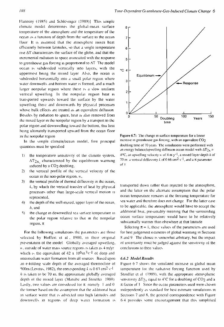
Figure 6.7: The change in surface temperature for a linear increase in greenhouse gas forcing, with an equivalent CO2 doubling time of 70 years The simulations were performed with an energy balance/upwelhng diffusion ocean model with AT2X = 4°C, an upwelling velocity M of 4 m y~', a mixed layer depth /; of 70 m a vertical diffusivity k of 0 66 cm2 s~l, and a n parameter of 1

transported down rather than rejected to the atmosphere, and the latter on the alternate assumption that the polar ocean temperature remains at the freezing temperature for sea water and therefore does not change For the latter case to be applicable, the atmosphere would have to accept the additional heat, presumably meaning that the surrounding ocean surface temperature would have to be relatively substantially warmei than elsewhere at that latitude

Selecting n = 1, these values of the parameters are used for best judgement estimates of global warming in Sections 8 and 9 The choice is somewhat arbitrary, but the impact of uncertainty must be judged against the sensitivity ol the conclusions to then values

6.6.2 Model Results Figuie 6 7 shows the simulated increase in global mean temperature foi the radiative forcing function used by Stouffer et al (1989), with the appropriate atmospheric sensitivity AT2x equal to 4°C for a doubling of CCb and a jr. factor of 1 Since the ocean parameters used were chosen independently as standaid for best estimate simulations in Sections 7 and 8, the general correspondence with Figure 6 4 piovides some encouragement that this simplified

6 Time-Dependent Gieenhouse Gas-Induced Climate Change 189

b

5

4

°C 3

2

1

n

DT2X = 4

1

5 — • / / D T a x = 2 5 ^

"1 DT2X = 1 5

l i 50 ^ . , 100 v 150

Doubling Years time

Figure 6.8: As for Figure 6 7 for a 7t parameter of 1 but for various values of atmospheric climate sensitivity AT2X

model is consistent with the ocean GCM Note, however, the slight upward curvature of the response in Figure 6 7, due to intermediate time scales of 20-100 years associated with heat diffusion or ventilation in the thermochne A tangent line fit at the 70 year mark could be described as a fractional response that is approximately 55% of the instantaneous forcing, with a slope of 66% superimposed on an offset of about 11 years For the sense in which the terms percentage response and lag are used here see Section 6 5 2

Figure 6 8 shows the simulated inciease in global mean temperature for the same radiative forcing but with atmospheric models of differing climate sensitivity For a sensitivity of 1 5°C for a doubling of CO2 the response fraction defined by the tangent line at 70 years is approximately 77% ol the instantaneous lorcing with a slope of 85% supci imposed on an offset of 6 years whereas for 4 5°C the concsponding values arc 52% 63% and 12 years

Figure 6 9 compaies the response for the standard parameter values with those for a jr. lactor of zcio and loi a purely diffusive model with the same diffusivity

Varying /; between 50 and 120 m makes very little diflerence to changes over several decades The effect of varying k between 0 5 and 2 0 cm^ s ' with historical forcing has been discussed by Wigley and Raper (1990) If k/w is held constant, the realized warming varies over this range by about 18% for AT2X = 4 5°C and bv 8% lor AT2X

= 1 5°C

Figure 6 10 shows the effect of terminating the inciease ol forcing after 70 years The response with JU = 1 continues to giow to a value conesponding to an oil set of some 10

7

6

5

°c 4

3

2

1

0

W = 4

<^

w

<6

y yy yy

,

y / / /

/ / W = 0 / / / /y y/ y y/ y y/ y y/ / yy y

y//—— w=4 77-=1 / /

i 1 50 _ . , 100

Doubling time

Years 150

Figure 6.9: As for Figure 6 7 but for w = 4,7t = 1 (corresponding to Response curve in Figure 6 7), w = 4 7t = 0, and w = 0 (dashed curve) Figure 6 7 shows the equilibrium case

H

3

C 2

1

0

y ^ " ^ 7 T = 0

/ ^ ^ 7 T = 1

I I I

Doubling time

100 200 Years

300

Figure 6.10: As for Figure 6 7 but for a forcing rising linearly with time until an equivalent C02 doubling after 70 years followed by a constant forcing

20 years, then rises very much more slowly to come to true equilibrium only after many centuries

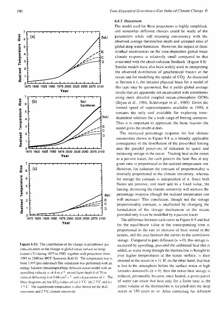
Also shown (Figure 6 11) are projections of future climate change using radiative forcing from IPCC Business-as-Usual and B-D emission scenarios, for values of the climate sensitivity AT2x equal to 1 5, 2 5 and 4 5°C These scenarios are discussed in the Annex Assuming k = 0 63 71 = 1 and w = 4 ms ' the realised wanning is 1 3 1 8 and 2 6°C (above pre-industnal temperatuies) undei the Business as Usual Scenario For Scenario B these estimates should be reduced by about 15%

190 Time-Dependent Gi eenhouse-Gas Induced Climate Change 6

BaU

1875 1900 1925 1950 1975 2000 2025 2050 2075 2100

Year

BaU

1875 1900 1925 1950 1975 2000 2025 2050 2075 2100 Year

1875 1900 1925 1950 1975 2000 2025 2050 2075 2100

Year

Iuj»ure 6.11: The contribution ot the change in greenhouse gas conccntiutions to the change in global-mean surface air temp erature (°C) during 187^ to 1985 together with projections from 198S to 2100 tor IPCC Scenarios BaU-D The temperature rise is from 176^ (pre-industnal) The simulation was performed with an energy balance climate/upwelhng diffusion ocean model with an upwellmg velocity \\ ot 4 m y~' mixed layer depth h ot 70 m vertical diltusivity k of 0 66 cm2 s ' and a Jt paiameter of 1 The thiee diagrams are toi AT2\-values ot (a) 4 5 C (b) 2 5 C and (c) 1 5 C The equilibrium tempeiature is also shown tor the BaU emissions and 2 VC climate sensitivity

6.6.3 Discussion The model used for these piojections is highly simplified, and somewhat different choices could be made of the parameters while still retaining consistency with the observed average thermochne depth and accepted rates of global deep water formation However, the impact ot these residual uncertainties on the time-dependent global mean climate response is relatively small compared to that associated with the cloud-radiation feedback (Figure 6 8) Similar models have also been widely used in interpreting the observed distribution of geochemical tracers in the ocean and for modelling the uptake of CO2 As discussed in Section 6 1, the detailed physical basis for a model of this type may be questioned, but it yields global average results that are apparently not inconsistent with simulations using more detailed coupled ocean-atmosphere GCMs (Bryan et al , 1984, Schlesinger et al , 1985) Given the limited speed of supercomputers available in 1990, it remains the only tool available for exploring time-dependent solutions for a wide range of forcing scenarios Thus it is important to appreciate the basic reasons the model gives the results it does

The increased percentage response for low climate sensitivities shown in Figure 6 8 is a broadly applicable consequence ot the distribution of the prescribed forcing into the parallel processes of radiation to space and increasing storage in the ocean Treating heat in the ocean as a passive tracer, for each process the heat flux at any given time is proportional to the teahzed temperature rise However, for radiation the constant of proportionality is inversely proportional to the climate sensitivity, whereas for storage the constant is independent of it Since both fluxes are positive, and must add to a fixed value, the lorcing, decreasing the climate sensitivity will increase the percentage response (though the realized temperature rise will increase) This conclusion, though not the storage proportionality constant, is unaffected by changing the formulation of the storage mechanism in the ocean, provided only it can be modelled by a passive tracer

The difference between each curve in Figure 6 9 and that for the equilibrium value at the corresponding time is proportional to the rate ol increase of heat stored in the oceans, and the area between the curves to the cumulative storage Compared to pure diffusion (w = 0), this storage is increased by upwelling, provided the additional heat that is added, as water rising through the thermochne is bi ought to ever higher temperatures at the ocean surface, is then retained in the ocean (K = 1) If, on the other hand, that heat is lost to the atmosphere before the surface watei in high latitudes downwells (71 = 0) then the ocean heat storage is reduced, presumably because, once heated, a given parcel of water can retain that heat only for a finite time as the entire volume of the thermochne is recycled into the deep ocean in 150 years or so After correcting foi diflerent

6 Time-Dependent Gieenhouse Gas Induced Climate Change 191

surface temperatures, the difference between these two curves measures for the case K = I the effective stoiage in the deep ocean below the thermocline, where the re­circulation time to the surface is many centuries The difference between n = 0 and the equilibrium, on the othei hand, measures the retention in the surface layers and the thermocline Though the latter aica is substantially larger than the former, it does not mean that all the heat concerned is immediately available to sustain a surface temperature rise

Figure 6 10 shows that within this model with n = 1, if the increase in forcing ceases abruptly alter 70 years, only 40% of the then unrealized global surface tempeiature increase is realized within the next 100 years, and most ol that occurs in the first 20 years If there is no heat storage in the deep ocean this percentage is substantially higher

It is thus apparent that the interpretation given in Section 6 5 3 of the results of Stouffer et al (1989) in terms of a two-layer box model is not unique However, it is re­assuring that broadly similar results emerge from an upwelling-diffusion model Nevertheless, it is clear that further coupled GCM simulations, different analyses of experiments already completed, and, above all, more definitive observations will be necessary to resolve these issues

6.7 Conclusions

Coupled ocean atmosphere general circulation models, though still of coarse resolution and subject to technical problems such as the flux adjustment are providing useful insights into the expected climate response due to a time-dependent radiative forcing However, only a very few simulations have been completed at this time and to explore the range of scenarios necessary for this assessment highly simplified upwelling-diffusion models of the ocean must be used instead

In response to a lorcing that is steadily increasing with time, the simulated global use of teinperatuie in both types of model is approximately a constant fiaction ol the equilibrium rise conesponding to the lorcing at an earlier time For an atmosphenc model vwth a tempciatuie sensitivity of 4°C loi a doubling ol CO2 this constant is appioximately 66% with an oil set of 1 1 years For a sensitivity of 1 5°C, the values aie about 85% and 6 years respectively Changing the paiameteis in the upwelling ditfusion model within ranges supposedly consistent with the global distribution of geophysical traccis can change the response fraction by up to 20% for the most sensitive atmospheric models but by only 10% loi the least sensitive

Indications from the upwelling diffusion model arc that if alter a steady use the lorcing weie to be held steady the response would continue to inciease at about the same rate for 10 20 years, but thciealtei would inciease only much

more slowly taking several centuries to achieve equilibnum This conclusion depends mostly on the ass­umption that 71 = 1, 1 e , greenhouse wanning in surface waters is transported downwards in high latitudes by downwelhng or exchange with deep water rather than being rejected to the atmosphere, and is thereafter sequestered for many centuries Heat storage in the thermocline affects the surface temperature on all time-scales, to some extent even a century or more later

There is no conclusive analysis of the relative role ol diffeient water masses in ocean heat storage foi the GCM of Stoufler et al (1990), but there are significant transleis of heat into volumes ol intermediate and deep water horn which the return time to the surface is many centuries Furthci analysis is required ol the implications loi tracer distributions of the existing simulations ol the cnculation in the control run, for comparison with the upwelling diffusion model Likewise, further simulations ol the fully interactive coupled GCM with different lorcing functions would strengthen confidence in the use ol the simplified tracer representation lor studies ol neai teim climate change

A sudden change of lorcing induces tiansient contrasts in surface temperature between land and ocean areas affecting the distribution ol precipitation Nevertheless the regional response pattern for both temperature and precipitation of coupled ocean-atmosphere GCMs tor a steadily increasing forcing generally resembles that foi an equilibrium simulation except uniformly reduced in magnitude Howevei, both such models with an active ocean show an anomalously large reduction in the use ol surface temperature around Antarctica and one shows a similai reduction in the noithern Noith Atlantic These anomalous regions aie associated with uipid vertical exchanges within the ocean due to convective oveiturning 01 wind driven upwelling downwelhng

Coupled ocean-atmosphere GCMs demonstuite an inherent interannual vailability, with a significant Iraction on decadal and longer timescales It is not clear how realistic current simulations ol the statistics of this variability really are At a given time warming due to gieenhouse gas lorcing is largest in high latitudes ol the northern hemisphere, but because the natuial vai lability is greatei there, the warming first becomes cleaily apparent in the tropics

The major sources ol unceilainty in these conclusions arise from inadequate observations to document how the piesent ocean circulation really functions Even fully mtei active GCMs need mixing parameters that must be adjusted ad lux to tit the real ocean and only when the processes controlling such mixing aie lull) understood and ieflected in the models can there be conlidencc in climate simulations under conditions substantially dilleient from the present day There is an urgent need to establish an

192 Time-Dependent Gi eenhouse-Gas-Induc ed Climate Change 6

operational system to collect oceanographic observations

routinely at sites all around the world ocean,

Present coarse resolution coupled ocean-atmosphere

general circulation models are yielding results that are

broadly consistent with existing understanding of the

general circulation of the ocean and of the atmospheric

climate system With increasing computer power and

improved data and understanding based upon planned

ocean observation programs, it may well be possible within

the next decade to resolve the most serious of the

remaining technical issues and achieve more realistic

simulations of the t ime-dependent coupled ocean-

atmosphere system responding to a variety of greenhouse

forcing scenarios Meanwhile, useful estimates of global

warming under a variety of different forcing scenarios may

be made using highly simplified upwelling-diffusion

models of the ocean, and with tracer simulations using

GCM reconstructions of the existing ocean circulation

References

Bryan, K , F G Komro, S Manabe and M J Spelman, 1982 Transient climate response to increasing atmospheric carbon dioxide Snence, 215, 56-58

Bryan, K , F G Komro, and C Rooth, 1984 The ocean's transient response to global surface anomalies In Climate Pi ocesses and Climate Sensitivity, Geophys Monogr Ser , 29 , J E Hansen and T Takahashi (eds ), Amer Geophys Union Washington, D C , 29-38

B r y a n , K , S Manabe, and M J Spelman, 1988 Interhemisphenc asymmetry in the transient response of a coupled ocean-atmosphere model to a CO2 forcing J Pin s Ocianoqi , 18,851 867

Harvey L D D and S H Schneider 1985 Transient climate response to external forcing on 10° 1()4 year time scales / Geophys Res, 90, 2191 2222

Hansen, J , 1 Fung, A Lacis, D Rind, S Lebedeff, R Ruedy, G Russell and P Stone, 1988 Global climate changes as forecast by the Goddard Institute tor Space Sciences three dimensional model / Geophys Ris 93,9341 9364

Hoffert, M 1 and B F Flannery 1985 Model projections of the time-dependent response to increasing carbon dioxide In Piojcctuii> the Climatic Effects of Inaeasim> Caibon Dioxide DOE/ER-0237, edited by M C MacCracken and F M Luther, United Stated Department of Energy, Washington, DC, pp 149 190

Hoffert, M I, A J Callegari, and C -T Hsieh, 1980 The role of deep sea heat storage in the secular response to climatic torcing J Geophys Res, 85 (CI 1), 6667-6679

Jones P D T M L Wigley C K Folland and D E Parker, I9S8 Spatial patterns in recent worldwide temperature trends Llimatt Momtoi 16 175 186

Karolv D 1989 Northern hemisphere temperature trends A possible greenhouse gas effect ' Giophw R(\ Lett 16 465 468

Levitus, S 1982 Climatological Atlas of the World Ocean, NOAA Prof Papers, 13, U S Dept of Commerce, Washington D C , 17311

Manabe S , and R J Stouffer, 1980 Sensitivity of a global climate model to an increase of CO2 concentration in the atmosphere J Geophys Res , 85, 5529-5554

Manabe, S K Bryan, and M J Spelman, 1990 Transient response of a global ocean-atmosphere model to a doubling of atmospheric carbon dioxide J Phvs Oceanogi , To be published

Manabe S 1990 Private communication Meehl, G A , and W M Washington, 1988 A companson of

soil-moisture sensitivity in two global climate models J Atmos Sci 45, 1476 1492

Meehl, G A , 1989 The coupled ocean-atmosphere modeling problem in the tropical Pacific and Asian monsoon regions J Chin, 2, 1146-1163

Rind, D , R Goldberg J Hansen, C Rosenzweig, and R Ruedy, 1989 Potential evapotranspiration and the likelihood of future drought / Geophys Res, in press

Sausen, R , K Barthel, and K Hasselmann, 1988 Coupled ocean atmosphere models with flux correction Clim Dyns, 2, 145-163

Semtner, A J and R M Chervin, 1988 A simulation of the global ocean circulation with resolved eddies J Geophys Res, 93, 15502 15522

Schlesinger M E 1989 Model projections of the climate changes induced by increased atmospheric CO2 In Climate and the Geo Sciences A Challenge foi Science and Society in the 21st Centwy, A Berger, S Schneider, and J C Duplessy, Eds , Kluwer Academic Publishers, Dordrecht, 375-415

Schlesinger, M E and X Jiang, 1988 The transport of CO2-mduced warming into the ocean An analysis of simulations by the OSU coupled atmosphere-ocean general circulation model Clim Dyn,l,\ 17

Schlesinger M E and J F B Mitchell, 1987 Climate model simulations of the equilibrium climatic response to increased carbon dioxide Ren Geophys 25,760 798

Schlesinger, M E W L Gates and Y -J Han, 1985 The role of the ocean in CO2 induced climate change Preliminary results from the OSU coupled atmosphere-ocean general circulation model In Coupkd Ocean Atmospheie Models, J C J Nihoul (ed), Elsevier Oceanography Series, 40, 447-478

Stouffer, R J S Manabe and K Bryan, 1989 Interhemisphenc asymmetry in climate response to a gradual increase of atmospheric carbon dioxide Native, 342, 660-662

Toggweiler, J R ,K Dixon and K Bryan, 1988 Simulations of Radiocarbon in a Coarse Resolution, World Ocean Model II Distributions of Bomb produced Carbon-14 J Geophys Res , 94(C 10), 8243-8264

Washington, W M , and G A Meehl, 1989 Climate sensitivity due to increased CO2 Experiments with a coupled atmosphere and ocean general circulation model Clim Dvn , 4, 1 38

Wetherald, RT and S Manabe, 1988 Cloud feedback processes in general circulation models J Atmos Sci 45(8), 1397 1415

Wigley, T M L , and S C B Raper, 1987 Thermal expansion of sea water associated with global warming Natiae, 330, 127-131

6 Time-Dependent Greenhouse Gas-Induced Climate Change J 93

Wigley, T. M. L., and S.C.B. Raper, 1989: Future changes in global-mean temperature and thermal-expansion-related sea level rise. In "Climate and Sea Level Change: Observations, Projections and Implications", (eds R. A. Warrick and T. M. L. Wigley) To be published.

Woods, J.D., 1984: Physics of thermocline ventilation. In: Coupled ocean-atmosphere circulation models. Ed. J.C.J. Nihoul, Elsevier.